Using Causal Discovery to Track Information Flow in Spatio-Temporal Data - A Testbed and Experimental Results Using Advection-Diffusion Simulations

Abstract

Causal discovery algorithms based on probabilistic graphical models have emerged in geoscience applications for the identification and visualization of dynamical processes. The key idea is to learn the structure of a graphical model from observed spatio-temporal data, which indicates information flow, thus pathways of interactions, in the observed physical system. Studying those pathways allows geoscientists to learn subtle details about the underlying dynamical mechanisms governing our planet. Initial studies using this approach on real-world atmospheric data have shown great potential for scientific discovery. However, in these initial studies no ground truth was available, so that the resulting graphs have been evaluated only by whether a domain expert thinks they seemed physically plausible. This paper seeks to fill this gap. We develop a testbed that emulates two dynamical processes dominant in many geoscience applications, namely advection and diffusion, in a 2D grid. Then we apply the causal discovery based information tracking algorithms to the simulation data to study how well the algorithms work for different scenarios and to gain a better understanding of the physical meaning of the graph results, in particular of instantaneous connections. We make all data sets used in this study available to the community as a benchmark.

Keywords: Information flow, graphical model, structure learning, causal discovery, geoscience.

1 Introduction

Recent research has shown great potential for causal discovery algorithms to track information flow from observed data for geoscience applications. The key idea for tracking information flow in geoscience is to interpret large-scale dynamical processes as information flow and to identify the pathways of this information flow by learning models from observational data. Since probabilistic graphical models are based on information-theoretical measures, they provide an ideal tool to track such information flow. We have obtained very promising results by applying structure learning of graphical models to real-world atmospheric data. For example we compared information flow in two case studies, (1) boreal winter vs. summer (Ebert-Uphoff and Deng (2012a)) and (2) current climate vs. projected climate in 100 years under global warming (Deng and Ebert-Uphoff (2014)), that provided new insights into the change of large-scale dynamics for these cases. (Obviously, the latter comparison is based on data generated by climate models, rather than observed data.)

One gap in our analysis so far has been that there is never any exact ground truth available in climate data, i.e. the only way to evaluate the results we obtained was to have the domain expert (second author of this paper) visually inspect the resulting graphs of information flow and consider whether they seemed physically plausible given the current knowledge in climate science about interactions in the atmosphere. While this evaluation confirmed the potential of this new methodology, it leaves much to be desired. In particular, we did not have the tools to evaluate the accuracy of the method or to know how exactly to interpret the resulting networks.

The same type of gap existed, until recently, for a different type of network learned from climate data, namely complex networks. Complex networks, also known as climate networks, were first proposed by Tsonis and Roebber (2004) and are a much simpler concept, exclusively based on Pearson correlation. Namely, any two nodes are connected if and only if the Pearson-correlation of the corresponding data is above a chosen threshold. (Note that the purpose of complex networks in geoscience applications is to identify similarities between different locations, while the purpose of the structure-learning networks is to identify interactions between different locations - a distinctly different purpose.) Complex networks have been applied to climate data for over a decade (Tsonis and Roebber (2004); Tsonis et al. (2006); Yamasaki et al. (2008); Tsonis et al. (2008); Donges et al. (2009); Steinhaeuser et al. (2010)), and many insights have been drawn from them over the years, but they had never actually been tested on simulation data until very recently. Molkenthin et al. (2014) finally filled this gap by testing complex networks on simulated data developed for that purpose and then comparing the results to the known physics of the simulation data.

Here we seek to achieve the same goal for structure-learning networks, which requires its own set of specific scenarios for testing. Namely, we develop a simulation framework that models the two most important dynamical processes in the atmosphere, diffusion and advection, allowing us to generate simulation data for a great variety of different conditions and for which the exact dynamics are known. We devise scenarios to test specific properties of the information tracking method for such dynamical processes. Each scenario consists of a choice of advection velocity field, advection and diffusion parameters, numerical parameters, spatial and temporal resolution, etc., and results in a data set. We apply information tracking algorithms to those data sets and report the results, then we use those results as a guide to the interpretation of results obtained from real-world data.

In addition we have created a supplemental website for this article that makes all of the resulting data sets, along with a description of the dynamic parameters, available to the community (see http://www.engr.colostate.edu/~iebert/DATA_SETS_CAUSAL_DISCOVERY/ ). We hope that these datasets can become benchmarks for researchers to explore and compare a variety of methods for information flow tracking, including graphical models, but also Gaussian models (Zerenner et al. (2014)) and Granger causal models (Arnold et al. (2007)). Having such benchmarks is important because (1) tracking information flow in spatio-temporal data generated from physical processes has not yet received much attention in literature; and (2) we believe that this area has significant applications in a large range of geoscience applications and thus will gain in importance in coming years.

1.1 Organization of This Article

The remainder of this article is organized as follows. The remainder of Section 1 describes the causal discovery algorithm used throughout this article and provides the motivating application for this study, namely tracking new insights about dynamical processes of our planet’s atmosphere. Section 2 describes how we generate data sets for testing, namely by using advection diffusion simulations. Section 3 presents results for three simple scenarios and Section 4 for three complex scenarios. Section 5 briefly discusses computational time. Section 6 discusses the results and suggests future work.

1.2 Algorithm Details

This section discusses the causal discovery method we have used in the past to track information flow in climate data and that is used here as well. We employ the well known framework of constraint-based structure learning of graphical models (Pearl (1988); Spirtes et al. (1993); Neapolitan (2003); Koller and Friedman (2009)). We use the PC stable algorithm (Colombo and Maathuis (2012, 2014)), which is a variation of the classic PC algorithm (Spirtes and Glymour (1991); Spirtes et al. (1993)). PC stable has several advantages, namely (1) it is order-independent, i.e. the order of variables does not affect the results; (2) it is more robust, i.e. mistakes early on cause less follow-up mistakes in the graphs; (3) it is easy to parallelize, thus reducing execution time.

The constraint-based structure learning yields independence graphs and we need to consider under which conditions these graphs can be interpreted to identify direct physical interactions, i.e. direct cause-effect relationships. Going from probability distribution (data) to independence graph, we have to make sure that the obtained independence graph actually models the data well, i.e. that it is faithful to the probability distribution. In our applications so far that is not a major concern. Even if faithfulness is violated we still seem to get decent results. Going from independence graph to causal interpretation, however, is a significant challenge, since we must ordinarily ensure that the nodes in the graph are causally sufficient, i.e. if any two nodes $X,Y$ of the graph have a common cause, $Z$, then $Z$ must also be included in the graph. In practice this condition is rarely satisfied in the geosciences, typically because some common causes may be unknown, hard to observe or including them all would make the model too complex. Some algorithms have been developed that can identify the existence of many hidden common causes (Spirtes et al. (1993)), but are of high computational complexity and currently not feasible for large graphs. Recent advances (Colombo et al. (2012)) may change that in the near future. Our approach is to simply not assume causal sufficiency, and to interpret the results accordingly. We accept that then we cannot prove causal connections, but we can disprove causal connections. Thus we can use an elimination procedure by first assuming that all variables are connected to each other, then disproving most of those connections until typically only few potential causal relationships are left at the end. Each one of those relationships may present a true causal connection, be due to a common cause or a combination of both.

Evaluation step: Thus we include a final evaluation step in our analysis. In the final graph, every link (or group of links) must be checked by a domain expert. If we can find a mechanism that explains it (e.g. from literature), the causal connection is confirmed. Otherwise, the link presents a new hypothesis to be investigated.

Scientific discovery: When seeking to learn new knowledge from data one interesting and common scenario is to have most links in the final graph confirmed from literature, thus confirming that the overall approach is correct, but also having a few unconfirmed links. The unconfirmed links are the ones that provide new hypotheses of causal connections and thus potentially new knowledge. Another scenario is to have the results confirm known mechanisms, but to provide quantitative information to the extend of the mechanism. For example, it is known that storm tracks move poleward in a warming climate, but we may be able to provide additional information on which locations are affected the most and how strong the effect is going to be, based on analyzing climate model data with this method.

Incorporating Spatial Dimensions: We use a grid to incorporate spatial dimensions. Any atmospheric field in the data, e.g. $X$, is represented by different variables, $X_{i}$, that represent its values at the $i$th grid point. While setting up the problem seems trivial at first, we showed in (Ebert-Uphoff and Deng (2014)) that the spacing between the measurement locations can result in artifacts in the resulting graphs, so proper grid spacing - or at least understanding the potential problems if proper spacing is not possible - is critical.

Incorporating Time: For many applications in geosciences temporal information plays a crucial role. For example, the climate system is very dynamic, with states at individual locations changing from day to day, but interactions often also taking days to travel from one location to another, while the strength of many signals decays significantly within days. Therefore for our applications taking time into account provided much stronger causal signals. In fact, for the climate science applications we considered, static models were unable to provide robust results, and we had to move to temporal models to be able to identify strong, robust causal signals (Ebert-Uphoff and Deng (2012b, a)). We believe the same holds for many physical systems in which temporal order is important. Another advantage of temporal models is that temporal information helps to establish causal directions.

To incorporate time explicitly into the modeling we use the approach first introduced by Chu et al. (2005), which adds lagged variables to the model. Since this approach does not seem to be widely known, we briefly outline it in Appendix A. Using that approach standard algorithms can be used to provide a temporal graphical model, but the price we pay for this is much higher computational complexity, since we are now dealing with $(N\cdot S)$, rather than $N$ variables, where $S$ is the number of time steps included in the model. Furthermore, as discussed in Ebert-Uphoff and Deng (2014), proper initialization of the first time slices is a critical issue, but one that can be resolved easily by calculating the model for more time slices than needed and then discarding the first few time slices in the results.

1.3 Sample Application: Tracking Information Flow in the Earth’ Atmosphere

A very promising application of causal discovery in climate science is to track the pathways of physical interaction around the globe. In order to do that we define a grid around the globe and evaluate an atmospheric field (such as temperature or geopotential height) at all grid points, which provides time series data at all grid points. Our approach is to then use the temporal version of PC stable to identify the strongest pathways of interactions around the globe based on the time series data (Ebert-Uphoff and Deng (2012a)). (Gaussian graphical models present an alternative approach for this purpose (Zerenner et al. (2014)) and Runge (2014) investigates this and other approaches.) No matter which method is used, the key idea is to interpret large-scale atmospheric dynamical processes as information flow around the globe and to identify the pathways of this information flow (physical interactions) using causal discovery.

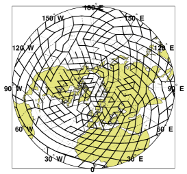
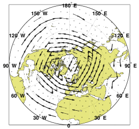
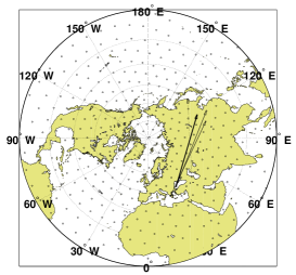
(a) $T=0$ days                     (b) $T=1$ day                     (c) $T=2$ days

Figure 1: Network plots for Northern hemisphere from PC stable ($D=1$ day, $\alpha=0.1$) based on Fekete grid with 800 grid points.

Figure 1 shows sample network plots obtained from atmospheric data using PC stable with $D=1$ day between time slices and significance level $\alpha=0.1$. The data used is daily NCEP-NCAR reanalysis data (Kalnay et al. (1996); Kistler et al. (2001)) for geopotential height at 500mb for boreal winter months (Dec-Feb) of years 1950-2000. Fig. 1(a), (b) and (c) show the strongest direct connections identified that take $0,1$ and $2$ days, respectively, to travel from source to target. These graphs were obtained by first generating temporal graphs with lagged variables, then converting them to summary graphs summarizing the strongest connections. It turns out that the interactions captured in Figures 1(b) and (c) are storm tracks. However, we were never able to fully understand the many interactions identified in Figure 1(a). What exactly do the apparently instantaneous connections between neighboring locations in Figure 1(a) represent?

This question was a strong motivation for the work reported in this article, namely to gain a better understanding of how exactly the underlying dynamical processes are represented in the network plots we obtain, with special emphasis on concurrent edges ($T=0$), i.e. those represented in graphs such as Figure 1(a). Furthermore, causal discovery algorithms have rarely been used (1) for spatio-temporal systems and (2) for physical systems. Studying advection and diffusion processes from simulations serves as an excellent benchmark to test such algorithms for those types of applications.

2 Generating Datasets for Testing

In our simulations we model two processes, advection and diffusion, in a two-dimensional grid. Advection and diffusion are common - and often dominant - processes in many dynamical processes in nature, especially in the geosciences. Advection is often described as a transport mechanism of a substance or property by a fluid (or air) due to the fluid’s bulk motion. An example is the transport of heat by a moving fluid. The motion of the fluid is described by a vector field that is constant over time, while the temperature is described by a scalar field that changes over time. In the context of this study, where we interpret changes of properties - such as temperature, pressure, etc. - as signals, we can think of an advection process as shifting a signal without changing the shape of the signal. In the language of image processing or digital filters, this can be understood as applying a pure translation filter, such as the convolution operator shown in Figure 2(a).

                          

(a) Advection-like filter                 (b) Diffusion-like filter

Figure 2: Examples of convolution filters corresponding to advection and diffusion processes.

In contrast, diffusion causes a signal to spread while the peak of the signal remains in place, e.g. any narrow wave of high amplitude is spread out into a wide wave with much lower amplitude. An example of diffusion would be to inject a small amount of hot water within a large amount of resting cold water, then diffusion would slowly spread the heat throughout the water until a new equilibrium (constant temperature throughout) is reached. In the language of digital filters, Fig. 2(b) provides a sample convolution filter for a diffusion process. The dominant processes in many geoscience applications can be modeled as a combination of both processes, advection to transport a signal and diffusion to spread it. Therefore we selected those two processes for our simulation framework.

2.1 Simulation Concepts and Parameters

While advection and diffusion can represent many processes in nature, here we focus on one physical scenario for illustrative purposes. We assume that we are modeling a moving fluid and the property of interest is the temperature at different locations over time. We denote as $f(x,y)$ the temperature at any point $(x,y)$. The motion of the fluid is described by a vector field, ${\bf V}(x,y)$, that specifies a velocity vector for any location $(x,y)$. $\kappa_{x}$ and $\kappa_{y}$ specify the diffusion coefficients in $x$ and $y$ direction. For $\kappa_{x}=\kappa_{y}=0$ there is no spreading of the signal, while increasing values of $\kappa_{x},\kappa_{y}$ indicate increased spreading of the signal. Appendix B reviews the corresponding partial differential equations governing the advection diffusion process and the numerical implementation thereof that we use to generate the simulation data. In this section we discuss only those concepts and parameters of the simulation that are necessary to understand the resulting data sets.

Numerical Grid: We use a rectangular grid for the numerical calculations. Its primary parameters are $\Delta t$, the time step for numerical calculation, and $\Delta x,\Delta y$, the distance between neighboring grid points in $x$ and $y$-directions.

Periodic Boundary Conditions: We use periodic boundary conditions to emulate the behavior of a large (infinite) system using just a small area. This means that we use a wrap-around in both x- and y-direction. For example, when reaching the right-most grid point in the x-direction, its neighbor to the right is defined to be the left-most grid point with the same y-coordinate, i.e. we jump from the last point in a row to the first point in the same row. The same applies in the upward (y-) direction.

The governing differential equation (Equation (3) in Appendix B), along with the periodic boundary conditions, and a set of initial conditions describing the temperature distribution at a time $t_{0}$, defines the temperature distribution over time. We can approximate this temperature distribution using a discrete grid, resulting in a numerical version of Equation (3). We use the first-order upwind scheme for the numerical implementation, which is described in detail in Appendix B.

Guaranteeing numerical stability: To keep the numerical calculations stable there are several conditions on how to choose the time step used in the numerical calculations, which depend on the advection velocity and diffusion coefficients used. For example, for pure advection and the 1-dimensional case the Courant-Friedrichs-Lewy (CFL) condition requires that the time step must be chosen such that

$$\Delta t\leq C\cdot\frac{\Delta x}{V_{max}},$$ (1)

where $C$, the Courant number, is between 0 and 1 ($0<C\leq 1$), and $V_{max}$ is the maximal absolute value of the velocity field. For the two-dimensional case we use the condition above with $V_{max}$ as the maximal magnitude of the velocity field and instead of $\Delta x$ we use the diagonal pixel length ($\sqrt{\Delta x^{2}+\Delta y^{2}}$) as a first guideline. The diffusion term has its own requirements for the time step, but those are not discussed here.

Numerical diffusion: In addition to the diffusion from the actual diffusion term, the numerical implementation creates additional diffusion effects, the amount of which depends on $C$ and other factors. In the special case where the advection velocity aligns with the vertical or horizontal grid directions, there is no numerical diffusion for $C=1$. Generally, numerical diffusion increases for decreasing values of $C$.

Signal speed and temporal resolution: $V_{max}$ is the maximal speed of the velocity field, and thus also the maximal signal speed - signal meaning in this context a change of temperature in the fluid -, since all signals travel with the fluid. As we have to obey Eq. (1) for numerical stability, it follows that we always have $\Delta tV_{max}\leq\Delta x$, i.e. the maximal distance traveled in one time step of the numerical calculations is always smaller than the width (diagonal length in 2D) of a grid pixel. In other words, the signal can never travel across more than one grid point at a time in the numerical calculations. Thus, in order to be able to experiment with higher signal speed for information tracking, i.e. signals crossing more than one grid point at a time, we may choose to only save data for every $M$th sample when generating data sets, i.e. the time step in the data file is $\widehat{\Delta t}=M\Delta t$. This procedure thus reduces the sample time after the numerical calculations are completed.

2.2 Information Sent to the System (Initial Conditions and Forcings)

The equilibrium state is for all grid points to have the same temperature. We send information (messages) to the system by injecting signals that disturb that equilibrium, either as initial conditions (IC) or as external forcings, then let the message pass through the system. The type of initial condition we use is as follows:

• Message Type 1: Single-point peak initial conditions (IC peak)
  First the temperature of a single grid point is set to a much higher value at a single time step, then we let the resulting signal propagate throughout the system until it dissipates. We send IC single-point peaks sequentially to all grid points, waiting for each signal to propagate, before restarting the system with initial conditions for the next grid point, thus creating as many consecutive runs as there are grid points.

Injecting a signal only at one point at a time assures that there is only a single signal propagating in the system at any given time. However, one potential problem with the peak approach is that for systems with high diffusion the signal may dissipate quickly and then there is no more signal left to track. Furthermore, real-world data sets are likely to include also other types of messages, such as continuous external forcing. Therefore we also include a second type of signal, continuous noise, as external forcing. We inject noise in two different ways:

• Message Type 2: Continuous single-point noise forcing (single-point noise)
  We feed normally distributed noise continuously to a single grid point. We do that for one run, then repeat for the next grid point. That assures that information is continuously fed to one grid point at a time. Even though the message (noise) is less crisp than a single high peak at that point, this method guards against the quick decay problem that can arise when feeding only a single peak.

• Message Type 3: Continuous all-point noise forcing (all-point noise)
  To make things more realistic, we can inject normally distributed noise continuously and simultaneously at all grid points.

Both the single-point and all-point noise are injected at every time step while the simulation is running, i.e. whatever noise is added at a grid point is transferred along with the rest of the signal at the next step. We call this prior noise, since it is added before the signal propagates in the simulation. An example of prior noise sources in real-world data is an un-modeled physical source of disturbances at grid points, such as spontaneously excited atmospheric convection over tropical oceans due to local convective instability, and large-scale disturbances that grow in midlatitudes as a result of hydrodynamic instability. Prior noise can be used as background noise in addition to a peak signal, or by itself as the primary signal.

In contrast, noise that is added to the time series after the simulation has completed we call posterior noise. That noise is not transferred according to the advection-diffusion equations and thus does not result in information transfer. An example of posterior noise sources in real-world data could be measurement errors that are fairly erratic. Posterior noise is not included in the simulations here, but can be easily added to the data sets provided by simply adding noise to the final signals.

2.3 Types of output edges and when we expect to see them

When interpreting the output of the causal discovery algorithm from spatio-temporal data, we distinguish three types of edges, (1) intra edges, (2) concurrent inter edges and (3) nonconcurrent inter edges. These edge types are explained below only for the advection-diffusion case, where the quantity of interest is temperature $f$. For the general case $f$ is simply substituted by any type of physical quantity considered or combinations thereof. In the following we denote as $f_{i}(x_{j},y_{k})$ the temperature at time $i$ at the grid point with coordinates $(x_{j},y_{k})$.

An intra edge connects the temperature $f_{i}$ at some location $(x_{j},y_{k})$ to the temperature at the same location at a later time:

$$\qquad f_{i}(x_{j},y_{k})\longrightarrow f_{{i}^{{}^{\prime}}}(x_{j},y_{k}),\quad\mbox{where}\;i^{{}^{\prime}}>i.$$

Intra edges encode the local memory (aka persistence in climate science) of a variable, i.e. for how long the current temperature at a location significantly affects the temperature at the same location. Note that by definition intra edges can only be nonconcurrent, i.e. not within the same time step.

An inter edge connects the temperature at some location to the temperature at a different location. Inter edges encode the information flow between different locations and thus track the remote impact of any location, i.e. its role in long-distance information transfer. Concurrent inter connections connect temperatures between different locations, but within the same time step, and thus generally end up being undirected (no arrow head) in our type of analysis (since we use temporal order to determine edge directions):

$$f_{i}(x_{j},y_{k})\;\hbox{---}\;f_{i}(x_{j^{{}^{\prime}}},y_{k^{{}^{\prime}}}),\;\mbox{where }\;j^{{}^{\prime}}\neq j\;\mbox{or}\;k^{{}^{\prime}}\neq k.$$

Nonconcurrent inter connections connect temperature between different locations and different times, and are directed from earlier time to later time.

$$f_{i}(x_{j},y_{k})\longrightarrow f_{i^{{}^{\prime}}}(x_{j^{{}^{\prime}}},y_{k^{{}^{\prime}}}),\;\mbox{where}\;i^{{}^{\prime}}>i\;\mbox{and}\;(j^{{}^{\prime}}\neq j\;\mbox{or}\;k^{{}^{\prime}}\neq k).$$

Expectations: Before we delve into the simulation results, we take a moment to formulate when we had expected the different types of edges to occur.

1. Intra edges: We expected intra edges to be dominant only for stationary processes and nearly stationary processes, i.e. in this context for pure diffusion or wherever advection velocities are very small.

2. Nonconcurrent inter edges: We expected nonconcurring inter edges to dominate for processes with significant velocities, i.e. in this context whenever there is significant advection velocity.

3. Concurrent inter edges: We expected concurrent inter edges to occur only for extremely high speeds, namely in cases where the signal moves across many grid points in a single time step, thus connections being so fast that they appear to be almost instantaneous.

As we will see in the following sections, while our expectations were confirmed for the first two edge types, the simulations provided some surprising new results concerning the occurrence and role of the third type, concurrent inter edges.

3 Simulation Results for Three Simple Scenarios

In this section we show results for three highly simplified scenarios, designed to test the information tracking algorithms when only one single type of process, or a very simple combination thereof, is present. The three simple scenarios are (a) pure diffusion, (b) pure advection and (c) mixed advection and diffusion. In those two cases involving advection the advection velocity field is trivial, namely, as shown in Fig. 3, the velocity is identical at each point and points straight to the right.

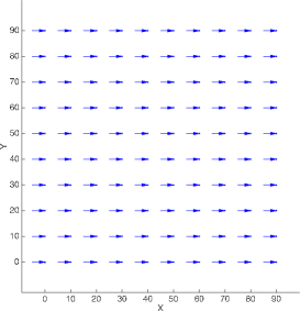
Figure 3: Vector field for advection displayed as displacement (in meters) within $\Delta t=5$ sec.

Once we understand the information flow signatures for these simple scenarios we move on to three more complex scenarios in Section 4 that incorporate both advection and diffusion and use more interesting and realistic advection velocity fields, representing different types of circular and cross current motion.

Parameters that are identical for all simulations are listed in Appendix C, while parameters specific to each scenario are listed in the corresponding sections. The supplemental website provides the corresponding data sets for all scenarios discussed in this article.

3.1 Types of Figures Generated

The results for each scenario are visualized in a single figure consisting of three types of plots, namely intra edge plots (top panels), inter edge plots (center panels) and velocity plots (bottom panels), see for example Figure 4. In intra edge plots (e.g. Figure 4(a)) each grid point is represented by a circle, which is empty if there is no intra edge, and filled if there is an intra edge. The filled circle is grey if the connection is very weak, otherwise it is blue. There are separate plots for different travel times, e.g. $T=\Delta t$ indicates connections across one time step, etc. For example, Fig. 4 (a) indicates that there are strong intra edges at all grid points, connecting each location to itself after 1, 2, 3 and 4 time steps, i.e. the local memory at each point is at least 4 time steps.

                 

$T=\Delta t$                        $T=2\Delta t$                        $T=3\Delta t$                        $T=4\Delta t$

(a) Intra edges

                 

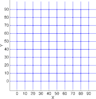
$T=0$                        $T=\Delta t$                        $T=2\Delta t$                        $T=3\Delta t$

(b) Inter edges

                          

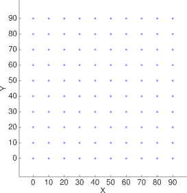
(c) Type 1 velocity estimate                            (d) Type 2 velocity estimate

Figure 4: Results for pure diffusion, 10x10 grid, $\kappa_{x}=\kappa_{y}=\kappa$, $M=1$.

The inter edge plots (e.g. Fig. 4 (b)) show the connections between different grid points. Concurrent edges are shown in the plot for $T=0$, and those edges are always undirected (no arrow heads), as seen for example on the left of Fig. 4 (b). Inter edge plots for $T>0$ show the nonconcurrent inter edges which are always directed (for an example see Fig. 7(b,c), as there are no such inter edges present in Fig. 4 (b)). Very weak inter edges are shown in grey, all other edges are shown in blue. Note that the scale in the inter plots is according to the time step in the data sets ($M\Delta t$), which may differ from the time step shown in the original advection velocity plots ($\Delta t$).

We generate two types of velocity estimate plots that combine the results of all directed edges found, taking the strengths of the connections into account. (See Ebert-Uphoff and Deng (2012b) for how we define the strength of each edge.) Note that the concurrent edges are ignored for now, since they have no direction and are thus hard to incorporate in velocity calculations. (We will return to the topic of concurrent edges in Section 4.) Velocity estimate plots show for each grid point the average direction of the incoming nonconcurring edges at that grid point, weighted by the strength of each edge. The difference is that Type 1 velocity plots use only nonconcurrent inter edges in the estimate, while Type 2 velocity include both nonconcurrent inter and intra edges. In these plots weak connections (i.e. those that result from only weak edges) are indicated by dashed lines, rather than grey color.

The purpose of Type 1 velocity plots is to highlight all pathways of information flow between different locations and those are often better visible when the intra edges are ignored. The idea behind the Type 2 velocity plot is that it can be compared to the original advection velocity plot used to generate the data. Note that there are subtle differences in the meaning of the original advection velocity and Type 2 velocity. The advection velocity field by definition only represents advection, not diffusion, while the Type 2 velocity plot represents the result for advection combined with diffusion. However, in the great majority of scenarios considered below, diffusion actually acts equally in all directions, so it should not impact the direction of information travel, but only magnitude. Furthermore, as we will see later, advection is the dominant process, thus the impact of diffusion on the magnitude of velocity is expected to be small wherever advection velocity is significant. Thus Type 2 velocity plots can be seen as an approximation of the input advection velocity fields. Both Type 1 and Type 2 velocity fields are scaled to be on the same scale as the original advection fields to allow for easy comparison.

We generally provide the full set of plots for each scenario, even if some of them show trivial or repetitive results, such as all intra edges being identical (Fig. 4(a)), no inter edges being present (three of the plots in Fig. 4(b)), or vanishing velocities (Fig. 4(c,d)). We provide those redundant plots nevertheless because it is much easier to visualize and compare results from different scenario, if all results are provided in a similar format, in this case a consistent set of plots.

3.2 Why Are No Error Measures Provided?

Eventually we plan to develop error measures that quantitatively evaluate the accuracy of the results for the different scenarios. However, at this point any effort in that direction appears premature, as we are just starting to learn about the behavior of the algorithm and even about which types of output figures to use in which case. Thus at this time qualitative visual representations of the output, i.e. figures, are much more useful than condensing the results to a single number. Furthermore, a primary use of the figures is for geoscientists to use them for scientific discovery of underlying dynamical mechanisms, and it is not trivial to assign a number to how well the output is suited to achieve that goal. Thus such measures will need to be carefully developed in the future in close collaboration with geoscientists, but that is a complex research topic of its own.

3.3 Results for Pure Diffusion

To study pure diffusion we temporarily drop the advection term in the diffusion advection equation, leaving only the diffusion term. Furthermore, we use $C=1$, so that there is no numerical diffusion. First we use Message Type 1, single peak initial conditions, without noise. We calculated results for two different grid resolutions, 10x10 and 20x20 grids, with varying temporal resolutions, $M=1,2,4$. In most cases we use $\kappa_{x}=\kappa_{y}=\kappa$, i.e. equal amount of diffusion in $x$ and $y$ direction. In some cases we use $\kappa_{x}=\kappa,\kappa_{y}=0$, to simulate diffusion only in $x$-direction.

Figure 4 shows results for a 10x10 point grid, $\kappa_{x}=\kappa_{y}=\kappa$, and $M=1$, i.e. full temporal resolution, while Figure 5 focuses on the concurrent inter connections for different values of $M$ and $\kappa_{y}$. Figures 4 and 5 use only Message Type 1. Figure 6 shows results when Message Types 2 and 3 are used instead.

Scenario	Concurrent inter edges for
	$M=1$	$M=2$	$M=4$
10x10 grid, $\kappa_{x}=\kappa$, $\kappa_{y}=\kappa$	Connections to $\pm x,\pm y$	Connections to $\pm x,\pm y$	Connections to $\pm x,\pm y$ and diagonals
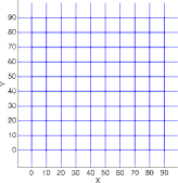
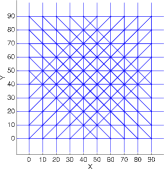
10x10 grid, $\kappa_{x}=\kappa$, $\kappa_{y}=0$	Connections to $\pm x$
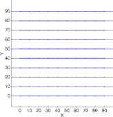
20x20 grid, $\kappa_{x}=\kappa$, $\kappa_{y}=\kappa$	No connections	Connections to $\pm x,\pm y$	Weak connections to $\pm x,\pm y$
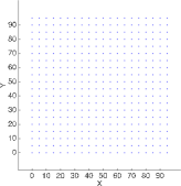
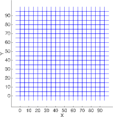
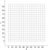
20x20 grid, $\kappa_{x}=\kappa$, $\kappa_{y}=0$	Weak connections to $\pm x$

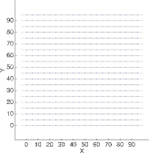
Figure 5: Concurrent inter edges for several pure diffusion experiments. Each point is connected to its 0, 2, 4, 5, 6, 7 or 8 closest neighbors.

                 

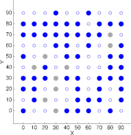
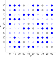
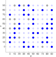
$T=\Delta t$                        $T=2\Delta t$                        $T=3\Delta t$                        $T=4\Delta t$

                 

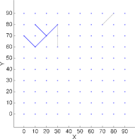
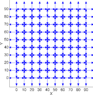
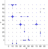
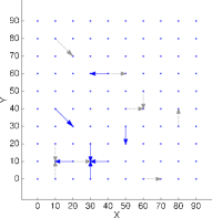
$T=0$                        $T=\Delta t$                        $T=2\Delta t$                        $T=3\Delta t$

(a) Intra (top) and inter (bottom) edges for single-point noise

                 

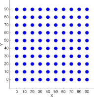
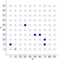
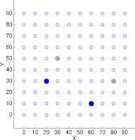
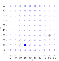
$T=\Delta t$                        $T=2\Delta t$                        $T=3\Delta t$                        $T=4\Delta t$

                 

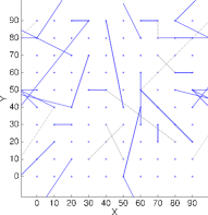
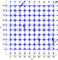
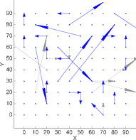
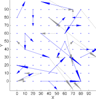
$T=0$                        $T=\Delta t$                        $T=2\Delta t$                        $T=3\Delta t$

(b) Intra (top) and inter (bottom) edges for all-point noise

Figure 6: Inter and intra edges for pure diffusion experiment, same parameters as in Fig. 4, but using single-point or all-point noise instead of single-point peaks. Type 1 and Type 2 velocity estimates (not shown) are close to zero throughout in both cases.

When using Message Type 1 (IC peak), we found that
(1) Intra edges are dominant, with local memory lasting several time steps, i.e. all locations have intra edges extending across $T=\Delta t,2\Delta t,3\Delta t$, etc.
(2) No inter edges occur for $T>0$.
(3) There may or may not be concurrent edges ($T=0$), see Figure 5. While for some grids no edges occurred, the more common scenario was the four-neighbor pattern, where each location connects to its 4 closest neighbors in the $\pm$x and $\pm$y directions. This occurred in most experiments for $k_{x}=k_{y}>0$, i.e. for equal diffusion in all directions. When diffusion was only in x-direction, i.e. $k_{x}>0,k_{y}=0$, each location connects only to its 2 closest neighbors in the $\pm$x direction.
(4) Both types of velocity plots report zero average velocities, which makes sense, since diffusion moves equally in all directions, i.e. the contributions cancel each other out.

When using Message Types 2 & 3 (prior noise) instead we found that
(1) For the majority of locations the local memory decreased (especially for all-point noise) to just one time step (see Fig. 6), but the intra edges are still strong for the first time step, $T=\Delta t$.
(2) The undirected edges found previously for $T=0$ shift completely to $T=\Delta t$, i.e. now there are neighboring directed edges pointing from each point to each neighboring point in x and y directions. These edges make sense, since diffusion also causes information transfer when a peak spreads to neighboring locations. That information transfer is just very slow and not traveling very far before decaying. That is probably the reason why it was not identified as directed edges in the IC peak case.
(3) Using noise as the only input signal creates several stray edges, especially for all-point noise.
(4) Type 1 and 2 velocity plots (not shown here) indicate that the estimated velocity is close to zero throughout, since the directed inter edges cancel each other out. There are only small non-zero values arising from the randomness in the noise.

Summary: For pure diffusion strong intra edges dominate as expected, while inter connections can be found between neighboring grid points, either as concurrent edges (Message Type 1) or as nonconcurring edges (Message Types 2 & 3). The estimated velocity throughout is near zero, which closely matches the zero advection velocity in this scenario.

3.4 Results for Pure Advection

Now we focus on tracking information flow in the pure advection scenario, i.e. we use $\kappa_{x}=\kappa_{y}=0$ and $C=1.0$. However, those parameters yield signals that never decay, and generate data that mimics purely deterministic relationships, which the causal discovery algorithm cannot handle. Since this is not a realistic scenario anyway, and we use it only for theoretical analysis, we did not change the algorithm and instead add a tiny amount of prior noise to the signal at each point at every time step (normally-distributed noise of small amplitude ($\sigma=0.1$), while the IC peaks have a large magnitude of $500$ units). Typical results using Message Type 1 are shown in Fig. 7, while results for Message Types 2 & 3 are shown in Figures 8 and 9.

                 

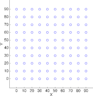
$T=\Delta t$                        $T=2\Delta t$                        $T=3\Delta t$                        $T=4\Delta t$

(a) Intra edges for pure advection and $M=1,2,4$: none.

                 

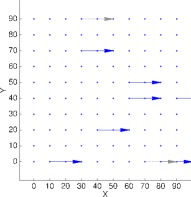
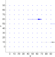
$T=0$                        $T=\Delta t$                        $T=2\Delta t$                        $T=3\Delta t$

(b) Inter edges for pure advection and $M=1$

                 

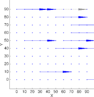
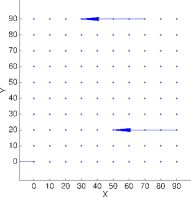
$T=0$                        $T=2\Delta t$                        $T=4\Delta t$                        $T=6\Delta t$

(c) Inter edges for pure advection and $M=2$

               

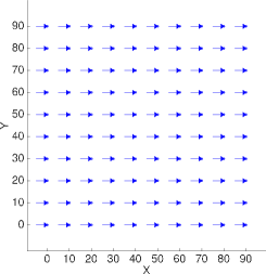
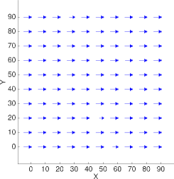
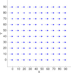
(d) Type 2 vel. for $M=1$           (e) Type 2 vel. for $M=2$           (f) Type 2 vel. for $M=4$

Figure 7: Results for advection experiments with $10\times 10$ grid points and different temporal resolutions ($M=1,2,4$). Velocity estimates (d,e,f) are scaled to $\Delta t=5$ sec and are identical with/without intra edges, since no intra edges were found.

                 

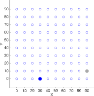
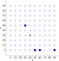
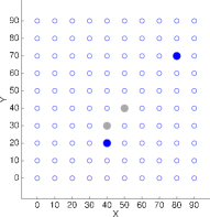
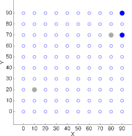
$T=\Delta t$                        $T=2\Delta t$                        $T=3\Delta t$                        $T=4\Delta t$

                 

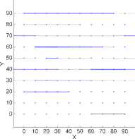
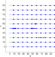
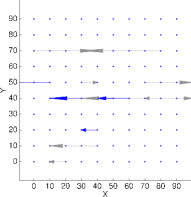
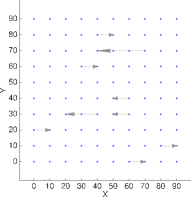
$T=0$                        $T=\Delta t$                        $T=2\Delta t$                        $T=3\Delta t$

(a) Intra (top) and inter (bottom) edges for single-point noise

                 

$T=\Delta t$                        $T=2\Delta t$                        $T=3\Delta t$                        $T=4\Delta t$

                 

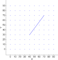
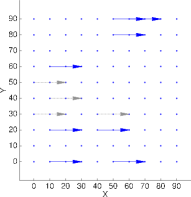
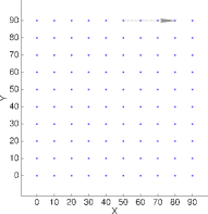
$T=0$                        $T=\Delta t$                        $T=2\Delta t$                        $T=3\Delta t$

(b) Intra (top) and inter (bottom) edges for all-point noise

Figure 8: Inter and intra edges for pure advection experiment, same parameters as in Fig. 7(a), but using single-point or all-point noise instead of single-point peaks.

                 

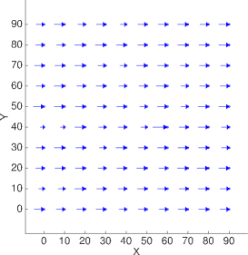
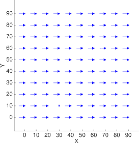
(a) Velocity estimate for single-point noise       (b) Velocity estimate for all-point noise

Figure 9: Type 2 velocity estimate for pure advection with continuous noise instead of peak initial conditions. Type 1 (not shown) and Type 2 are practically indistinguishable, since only very few intra connections exist.

When using Message Type 1 (IC peak), we found that
(1) There are no intra edges.
(2) There are no concurrent inter edges. This even holds for $M\geq 10$ (not shown here).
(3) The great majority of inter edges occur for $T=\Delta t$. The length of connection is one grid point per time step, i.e. 1 grid point for $T=\Delta t$, 2 grid points for $T=2\Delta t$, etc. This even holds for $T\geq 10\Delta t$ (results not shown here). This length is expected, since we use $C=1$, i.e. signals travel exactly one grid point per time step in this scenario. Note that for $T=6\Delta t$ in Fig. 7(b), the length of the connections is 6 grid points, but since each row only has 10 grid points, it appears as if locations connect 4 points to the right, rather than 6 points to the right. Also note, that the asymmetric inter edges that occur for $T>\Delta t$, are all due to the fact that even for Message Type 1 we use a small amount of noise (see previous paragraph). Otherwise we would not see these longer edges, which describe an echo effect, since they basically duplicate the direction and speed of the edges found for $T=\Delta t$.
(4) Type 1 and Type 2 velocity estimates are identical, since there are no intra edges. They are very good for M=1, 2, with a few incorrect magnitudes for M=4.

When using Message Types 2 & 3 (prior noise), we found that
(1) The overall signature with prior noise is quite similar to the ones with the strong initial conditions, especially for all-point noise.
(2) Results for all-point noise are considerably better than for single-point noise. The reason is probably that with all-point noise the algorithm has more non-zero signals to work with at any time.
(3) No intra edges appear for all-point, a few for single-point noise. Likewise single-point noise results have more stray inter edges, while all-point noise has few.

Summary: In the pure advection experiments there are very few intra connections and the nonconcurring inter edges are dominant, as expected. Velocity plots show decent estimates of the original advection field for all message types used.

3.5 Results for simple scenario combining advection and diffusion

Now we briefly consider what happens if both advection and diffusion are present. Since diffusion is present, there is no need to add noise when using single peak initial conditions. However, we encountered issues with numerical stability with this combination and thus chose a lower value, $C=0.7$, to make sure the numerical simulations are stable. This also adds additional diffusion in the simulation, thus enhancing the effect of diffusion. Furthermore, it reduces the signal speed to 0.7 grid points per time step.

Fig. 10 shows results for Message Type 1. We found that the results are very similar to the ones observed for advection only, which means that the advection process is clearly dominant. In fact no intra edges are found, in spite of the presence of the diffusion, plus the additional numerical diffusion from choosing $C=0.7$. The primary difference between these results (Fig. 10) and the ones for pure advection (Fig. 10) is that there are now also many inter edges for $T>\Delta t$. These are again echo edges, repeating the edge direction and speed for $T=\Delta t$ at larger time spans. In this case they are due to diffusion. The directions in the velocity estimates (Type 1 and Type 2 velocity estimates are identical, since there are no intra edges) appear to be correct, but the magnitudes are inflated, due to the echo edges, which contribute the same information multiple times. In summary, the large number of echo edges is the most interesting fact here. Whenever that happens one may consider to only use the inter edges up to $T=\Delta t$ to generate velocity plots.

                 

$T=\Delta t$                        $T=2\Delta t$                        $T=3\Delta t$                        $T=4\Delta t$

(a) Intra edges

                 

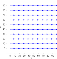
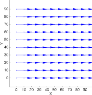
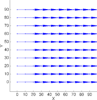
$T=0$                        $T=\Delta t$                        $T=2\Delta t$                        $T=3\Delta t$

(b) Inter edges

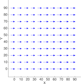
(c) Type 1 Velocity Estimate (Type 2 looks identical)

Figure 10: Results for simple scenario with advection and diffusion combined, same parameters as in Fig. 7, but using diffusion term, $M=1$ and $C=0.7$.

4 Simulation Results for Three Complex Scenarios

Now we define three more complex scenarios to test the structure learning from complex spatio-temporal data. The key feature of these scenarios is that the advection velocity fields no longer align with the horizontal or vertical direction of the grid and that their magnitude also varies by location. Thus these scenarios are suitable to test the effects of (1) varying orientation of arrow direction, i.e. no longer aligning with the grid; (2) varying magnitude of arrows. Furthermore, each scenario has some additional features that make it interesting for testing certain effects.

Scenario 1: The advection for Scenario 1 is defined by the rotating ring flow shown in Figure 11(a). The special feature of Scenario 1 is that the velocities are set to exactly zero in large areas, namely anywhere inside and outside of the ring. Thus Scenario 1 is designed to also test the effect of large areas with zero advection velocity, i.e. pure diffusion in those areas.

Scenario 2: The advection for Scenario 2 is defined by the rotating vector field shown in Figure 11(b).

     

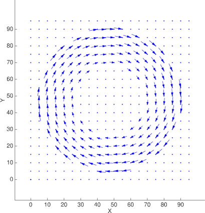
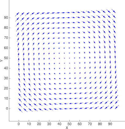
(a) Scenario 1                                             (b) Scenario 2

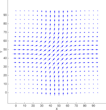
(c) Scenario 3

Figure 11: Advection Velocity Fields for Scenarios 1, 2 and 3.

Note that the magnitude of the vectors is proportional to the distance from the center, i.e. velocities vanish near the center and are largest at the boundaries. Furthermore, the periodic boundary conditions cause strong discontinuities of the velocity directions near the boundaries. For example, at the center of the upper boundary of Fig. 11(b) the velocities are straight to the right, while at the center of the bottom boundary the velocities are straight to the left, i.e. the velocities at these wrap-around neighboring points are exactly opposite of each other, mimicking the occurrence of counter currents. The same effect occurs at the centers of the right and left boundary. Thus there is a 180 degree angle between the velocity vectors at wrap-around at the centers of all four boundary lines. This angle decreases to about 90 degrees towards the four corners, thus it remains significant. Thus Scenario 1 is designed to test the effect of counter currents and other abrupt changes in velocity direction.

Scenario 3: The advection for Scenario 3 is motivated by the cross current velocity field used by Molkenthin et al. (2014) to test their correlation networks. Scenario 3 emulates two crossing currents as shown in Figure 11(c). One current flows from left to right, the other from bottom to top, with velocities increasing exponentially toward the center of the grid. Even though velocities are small outside of the two main currents, there are no true zero velocities in this case. Furthermore, in contrast to Scenario 1 the directions in Scenario 3 are all consistent at the boundaries (no sudden changes).

Other parameters for Scenarios 1-3: Each grid consists of $20\times 20=400$ points. As before, the advection velocity field is scaled for each scenario so that the maximal velocity is $1$ $m/s$ and diffusion is set to $\kappa_{x}=\kappa_{y}=1$ $m^{2}/s$. The numerical stability parameter is chosen as $C=0.5$, which yields significant additional diffusion. All results reported here are for Message Type 1 (IC peak) and no prior noise is used.

4.1 Results for complex scenarios when concurrent edges are allowed

           

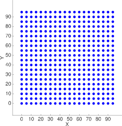
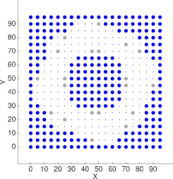
$T=\Delta t$                                $T=2\Delta t$                                $T=3\Delta t$

(a) Intra edges

           

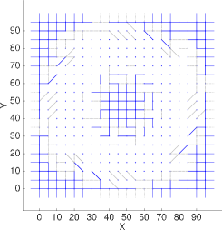
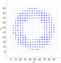
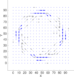
$T=0$                                $T=\Delta t$                                $T=2\Delta t$

(b) Inter edges

  

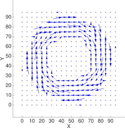
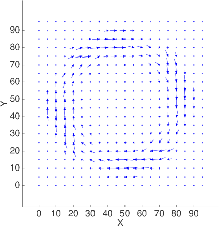
(c) Velocity estimated without intra edges           (d) Velocity estimated with intra edges

Figure 12: Results for Scenario 1 with concurrent edges allowed.

Results for Scenario 1 (Fig. 12):
(1) There are more intra edges than expect for $T=\Delta t$. Starting at $T=3\Delta t$ we see the pattern we expected, namely intra edges only where advection velocity is low.
(2) Inter edges for $T\geq\Delta t$ show good approximation of the original advection field, with most of the edges present for $T=\Delta t$. Likewise the velocity estimates give a good indication of the shape of the original advection field.
3) Concurrent inter edges (T=0) occur in all locations where diffusion dominates (areas with zero advection velocity). No surprise there.

Results for Scenario 2 (Fig. 13):
(1) Intra edges occur where advection velocity is smallest, as expected.
(2) Inter edges for $T=\Delta t$ capture most of the advection velocities, but one can see the increasing difficulty of using a rectangular grid to represent diagonal velocity vectors.
(3) The velocity plot of Type 1 (without intra edges) gives a good indication of the original velocity field, but (1) with directions distorted to align with the grid, and (2) with inflated magnitudes. The velocity plot of Type 2 (taking intra edges into account) is better at detecting the high speed advection areas, but drops the connections in the low velocity areas almost completely.
(4) The concurrent inter edges are very interesting (left-most panel in Fig. 13). The connections towards the center are expected, because diffusion is dominant there. However, the connections toward the boundary are a new effect. These are probably due to the contradictory velocities at the boundaries of the advection field of Scenario 2, and will be discussed more later.

           

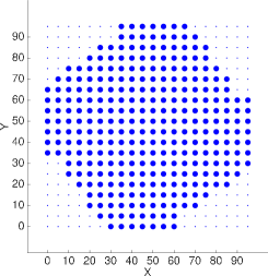
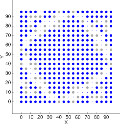
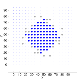
$T=\Delta t$                                $T=2\Delta t$                                $T=3\Delta t$

(a) Intra edges

           

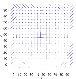
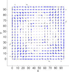
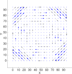
$T=0$                                $T=\Delta t$                                $T=2\Delta t$

(b) Inter edges

  

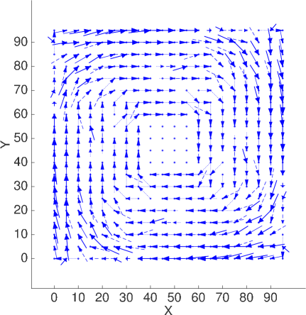
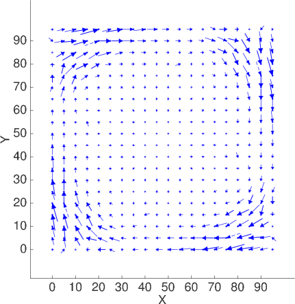
(c) Velocity estimated without intra edges           (d) Velocity estimated with intra edges

Figure 13: Results for Scenario 2 with concurrent edges allowed.

           

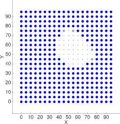
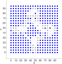
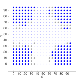
$T=\Delta t$                                $T=2\Delta t$                                $T=3\Delta t$

(a) Intra edges

           

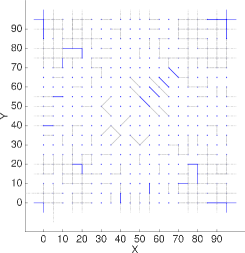
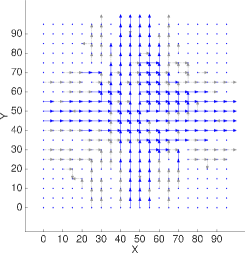
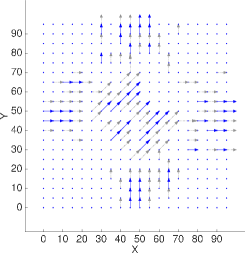
$T=0$                                $T=\Delta t$                                $T=2\Delta t$

(b) Inter edges

  

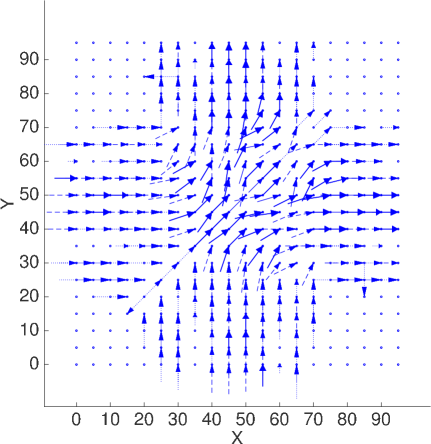
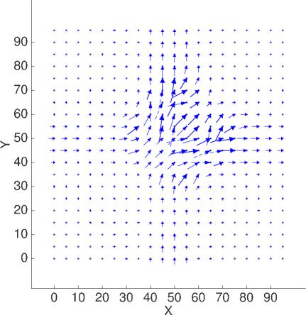
(c) Velocity estimated without intra edges           (d) Velocity estimated with intra edges

Figure 14: Results for Scenario 3 with concurrent edges allowed.

Results for Scenario 3 (Fig. 14):
(1) Just as in Scenario 1, there are more intra edges than expected for $T=\Delta t$, with the pattern we expected only emerging for $T=3\Delta t$.
(2) The inter edges for $T=\Delta t$ again capture the original advection field, but with some problems in some areas where the velocity is diagonal to the grid.
(3) There are again interesting concurrent edges (left-most panel in Fig. 14(b)), not only where advection velocity is small, but also near the center, which is exactly where the other inter edges have problems representing some diagonal edges.
(4) The difference between Velocity 1 and 2 plots is again significant. Just as in previous cases, the Velocity 1 plot is more sensitive, i.e. catches more edges, but the amplitudes are inflated, while the Velocity 2 plot is better at estimating velocity magnitudes, but misses some of the smaller connections.

A lesson learned: Velocity 1 plots are indeed better to detect connections that have lower speeds, i.e. they have much higher sensitivity. Velocity 2 plots are better at identifying the fastest connections and estimating actual speeds. By definition the directions in both plots are always the same, just the magnitudes change.

4.2 Results for complex scenarios when concurrent edges are excluded

Concurrent edges play an odd role, because they are the only edges that are not directed, thus provide less useful information about the underlying physical mechanisms, and cannot be included in the velocity estimates. In this section we consider what happens if we exclude the concurrent edges a priori, i.e. if we run the causal discovery algorithm with the prior knowledge that edges within the same time slice are forbidden (see Appendix A for details on how to do that). How do the results change? Does a priori excluding concurrent edges result in significant new inter edges for $T>0$ and, if so, what do those new edges look like?

For brevity, here we only show results for the velocity estimates. Figures 15 to 17 show the velocity estimates for Scenarios 1-3 when concurrent edges are a priori excluded. These can be directly compared to Figs. 12 - 14 where concurrent edges are allowed. For Type 1 velocity estimates we see that new edges appear primarily in areas where previously concurrent edges were present. For Scenarios 2 and 3, excluding the concurrent edges a priori seems to result in an improvement, since it increases the sensitivity of the Type 1 plots, i.e. we now pick up connections corresponding to even lower advection velocities. For Scenario 1, however, it seems that the sensitivity is too high, namely creating connections where there should not be any, because the original advection velocities are truly zero. Scenario 1 is the only one with advection velocities truly zero anywhere, so this is likely the reason we see this negative effect only there. In contrast, for Type 2 velocity estimates the results when concurrent edges are excluded are almost indistinguishable from those when concurrent edges were included. This indicates that the concurrent edges were often weak and only occurred in areas where intra edges are dominant, thus once we take intra edges into account, there is no significant difference between the corresponding results.

  

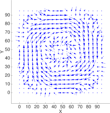
(a) Velocity estimated without intra edges           (b) Velocity estimated with intra edges

Figure 15: Results for Scenario 1 when concurrent edges are a priori forbidden.

  

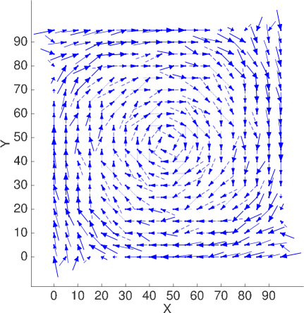
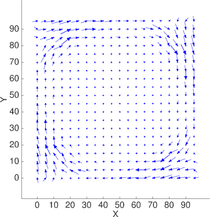
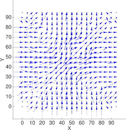
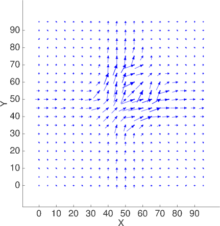
(a) Velocity estimated without intra edges           (b) Velocity estimated with intra edges

Figure 16: Results for Scenario 1 when concurrent edges are a priori forbidden

  

(a) Velocity estimated without intra edges           (b) Velocity estimated with intra edges

Figure 17: Results for Scenario 3 when concurrent edges are a priori forbidden.

4.3 Results for complex scenarios when signal speed is increased

           

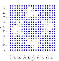
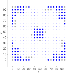
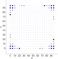
$T=4\Delta t$                                $T=8\Delta t$                                $T=12\Delta t$

(a) Intra edges

           

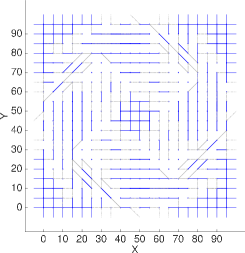
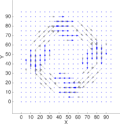
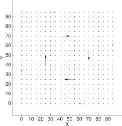
$T=0$                                $T=4\Delta t$                                $T=8\Delta t$

(b) Inter edges

  

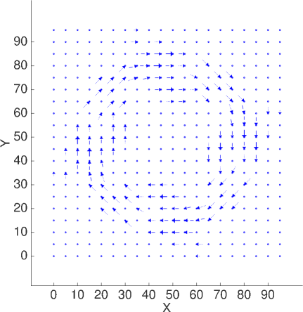
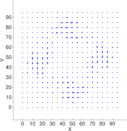
(c) Velocity estimated without intra edges           (d) Velocity estimated with intra edges

Figure 18: Results for Scenario 1 with concurrent edges allowed and $M=4$.

           

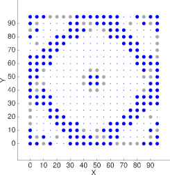
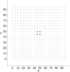
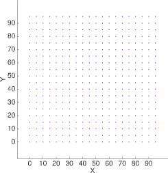
$T=10\Delta t$                                $T=20\Delta t$                                $T=30\Delta t$

(a) Intra edges

           

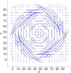
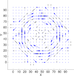
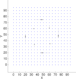
$T=0$                                $T=10\Delta t$                                $T=20\Delta t$

(b) Inter edges

  

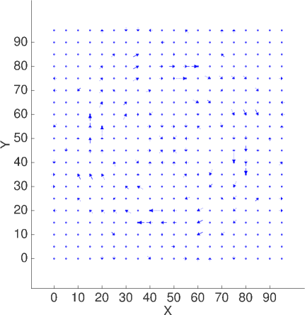
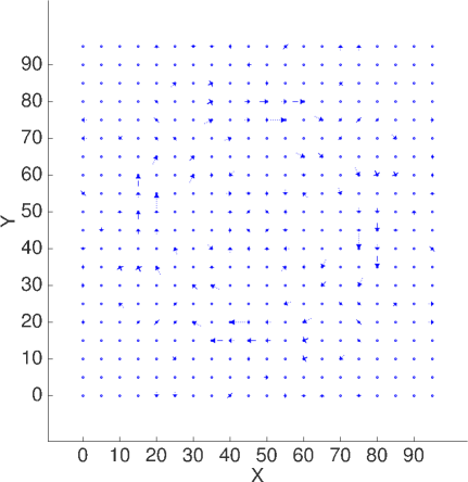
(c) Velocity estimated without intra edges           (d) Velocity estimated with intra edges

Figure 19: Results for Scenario 1 with concurrent edges allowed and $M=10$.

The last set of results discussed here briefly investigates what happens in the complex scenarios if we increase signal speed, i.e. if signals travel several grid points per time step. Since numerical stability prevents us from increasing the travel speed beyond one grid point per time step in the numerical calculations, we instead reduce the temporal resolution after the numerical calculations are finished, by keeping only data for every $M$th time step of the numerical calculations. Figures 18 and 19 show the results for Scenario 1 for $M=4$ and $M=10$, which can be compared directly to the results for $M=1$ shown in Fig. 12. It is clear that for increasing $M$ the number of intra edges declines rapidly. Much more interesting, however, is the drastic change to the concurrent inter edges. For $M=1$ the concurrent edges only occur in areas with zero advection velocity. On the other extreme, for $M=10$, many of the concurrent edges actually represent high speed advection connections - an effect we had expected to see, but were unable to confirm in simulation results until now! For $M=4$ we see a mixture of effects, i.e. some of the concurrent edges are due to diffusion (recognizable from the connectivity along the grid lines to all neighbors) and some represent high-speed advection (recognizable by their alignment with the pattern for directed intra edges). Since concurrent edges are not included in the velocity estimates, as information from directed inter edges ($T>0$) move to concurrent inter edges ($T=0$) for increasing $M$, that information no longer makes it into the velocity plots. Thus the resulting velocity estimates are getting weaker, a bit for $M=4$, and much more so for $M=10$. In summary, these results demonstrate the varying roles of concurrent inter edges, and the importance of not simply dropping concurrent edges without analyzing first which roles they play and what they may tell us about the underlying dynamical mechanisms, especially in cases where the velocity estimates are extremely sparse.

5 Computational Time

Almost as interesting as the actual connectivity results for the different scenarios presented in the previous sections is the tremendous difference in calculation time just based on the input data and parameter choices. To demonstrate this Table 1 shows results for the simple scenarios of pure diffusion and pure advection discussed in Section 3. In all cases we have the same number of variables (100 grid points $\times$ 20 tiers = 2,000 graph nodes), and identical temporal constraints (an effect cannot occur before its cause, i.e. we allow concurrent edges). The only difference is whether the simulation data comes from diffusion or advection and what type of messages we feed in, so purely the physics of the problem.

As seen in Table 1, causal discovery is always drastically faster (at least 50 times) for advection data than for diffusion data. Note for advection how quickly the number of remaining edges drop down to just a few thousands by the time the CI tests of order 0 are completed, i.e. by just using simple pair-wise correlation. This means that for advection the algorithm very quickly narrows down the possibilities to a small set of connections, which drastically reduces computational cost. In contrast the diffusion case shows a very different behavior. Since signals diminish quickly with diffusion, the algorithm is not able to narrow down the possibilities early on to a small set of connections. Even when using IC peak signals there are still over 100,000 edges left after all order 1 tests are completed, while the final number of edges is 6,300. In summary the results clearly demonstrate that advection is much easier to track than diffusion, both in terms of time and robustness to signal strength. Namely, advection signals are quick to be found and can be found even if no strong signals are sent into the system, only noise.

Type	Input signal	Order	# CI tests	# edges left	Total
		of CI tests	performed	after completion	time
Diffusion	IC peak	0	1,999,000	1,927,800
	(Message Type 1)	1	1,313,986,814	101,100
		2	198,823,873	22,650
		3	21,759,968	9,150
		8		6,300	1.7 min
Diffusion	Single-point noise	0	1,999,000	1,996,774
	(Message Type 2)	1	3,432,381,850	1,120,533
		2	266,615,933,633	86,128
		3	12,085,420,716	16,417
		13		12,949	5.6 hrs
Diffusion	All-point noise	0	1,999,000	1,961,485
	(Message Type 3)	1	3,386,500,452	1,336,309
		2	483,241,883,491	164,025
		3	58,994,333,551	31,271
		12		12,225	12.1 hrs
Advection	IC peak (w. small noise)	0	1,999,000	19,000
	(Message Type 1)	1	245,912	1,969
		2	65	1,969
		3	0	1,969
		3		1,969	$<1$ sec
Advection	Single-point noise	0	1,999,000	145,481
	(Message Type 2)	1	5,838,246	4,138
		2	33,847	3,065
		3	15,493	3,039
		9		3,027	1 sec
Advection	All-point noise	0	1,999,000	633,393
	(Message Type 3)	1	26,330,092	3,334
		2	801,173	3,195
		3	4,243,287	3,090
		22		2,817	13.8 min

Table 1: Computational time of PC stable for pure diffusion and pure advection. Listed are the number of conditional independence tests performed by PC stable for $order=0,1,2,3$ and how many edges are left at the end of those tests. For each experiment the last row lists the maximal order considered by PC stable, the final number of edges of the skeleton and the total time to calculate the skeleton.

Finally, Table 2 compares some results for different scenarios with or without concurrent edges allowed. For that comparison we are interested in both the computational effort and the final number of edges, which indicates the model complexity. Excluding concurrent edges means that we include more prior knowledge, namely that nodes may not be connected to other nodes within the same time slice. One may think that this additional knowledge, which limits the edges that can be considered, would always reduce computational time. However, over the years we have often found the opposite to be true. Namely, if the prior knowledge forbids edges that are crucial to the model, then those edges may be replaced by a large number of substitute edges and the final model is more complex, i.e. containing a larger number of connections. Furthermore, while lower computational time indicates a simpler model, which is usually preferred, one has to be more careful about interpreting the final number of edges. An increase in the number of edges may indicate either an unnecessary increase in complexity, or it may indicate an increased sensitivity, i.e. that more valid connections are picked up. Which one is the case needs to be determined in each case. Table 2 lists the number of edges and computational time for several different scenarios. For the case where concurrent edges are allowed, the numbers in parentheses split the total number of edges into the number of concurrent plus nonconcurrent edges. For the pure advection scenario ($M=1$) the results are identical whether concurrent edges are allowed or not, since no concurrent edges are found either way. This is also true for $M=2$ and $M=4$ (not shown in table). For Complex Scenarios 1-3 the computational effort and number of edges are extremely similar when concurrent edges are allowed vs. forbidden. A possible explanation is that all complex scenarios are dominated by advection at most grid points, thus behave more like pure advection scenarios. The most interesting case is pure diffusion. While there is not much difference for $M=1$, computational time starts to increase when concurrent edges are forbidden for $M=2$ and becomes overwhelming for $M=4$. (In fact, the calculations for $M=4$ never finished - we stopped them after 2 weeks.) However, while computational time is much higher when concurrent edges are forbidden, we did not see any case (yet) where the actual number of edges increases drastically - in fact so far the total number of edges was always lower, with the number of non-concurrent edges going up slightly. It just seems to take longer - in some cases prohibitively longer - to calculate the model when concurrent edges are forbidden. However, one needs to keep in mind that the computational time is likely to be quite different for other methods, such as Gaussian models or Granger causal methods. Clearly, more research needs to be done on the advantages and disadvantages of including concurrent edges in the modeling process - and on the exact role of the concurrent edges in the final model.

	Concurrent allowed		Concurrent forbidden
Scenario	# edges	time	# edges	time
	(conc. + non-conc.)
Diffusion (M=1)	6,300 (800 + 5,500)	96 sec	5,700	106 sec
Diffusion (M=2)	8,400 (1,400 + 7,000)	2.6 min	8,200	31.4 min
Diffusion (M=4)	6,000 (1,500 + 4,500)	14.2 min	$\leq$ 9,500	$\geq$ 14 days
Advection (M=1)	1,969 (0 + 1.969)	$<$ 1 sec	1,969	$<$ 1 sec
Complex Scenario 1	24,050 (2,742 + 21,308)	1.7 hrs	22,520	1.6 hrs
Complex Scenario 2	14,304 (2,424 + 11,880)	1.4 hrs	13,392	1.3 hrs
Complex Scenario 3	18,696 (2,438 + 16,258)	1.7 hrs	17,943	1.6 hrs

Table 2: Computation time and final number of edges when concurrent edges are allowed vs. forbidden. All results are for single peak initial conditions. (Given in parentheses is the number of concurrent, plus the number of nonconcurrent edges.)

6 Discussion and Future Work

The scenarios provided in this article provide a very rich playground to test a variety of structure learning algorithms on spatio-temporal data. The properties of the graph structure to be discovered varies tremendously with the physical process chosen to generate the data (e.g. diffusion vs. advection), but also with algorithm choices, such as whether to allow concurrent edges or not. It will be very interesting to compare results for alternative methods of structure learning for these scenarios, such as Granger causal models and Gaussian models. In particular we hope that comparing results from Granger, Gaussian and Graphical models will help us gain a better intuitive understanding of the inherent differences between those algorithms, in particular of their strengths and weaknesses for such geoscience applications. Some of the algorithms are expected to be much faster than the graphical model approach used here, but are their results comparable in quality to the ones obtained here? Is their sensitivity, accuracy and robustness better or worse than for the algorithm discussed here? Are some of the alternatives maybe better for some types of processes (e.g. high-speed signals or maybe scenarios where concurrent edges can be ignored) and worse for others? To the best of our knowledge the three types of algorithms have never been rigorously compared for structure learning from spatio-temporal data and these scenarios provide a perfect platform for comparison.

One of the most important lessons we learned about the interpretation of the results from the current approach concerns the concurrent edges. The different roles that concurrent edges can play in this context are fascinating and clearly deserve further study in the future. Concurrent inter edges can occur for reasons we did not realize before. We had assumed that concurrent inter edges always represent extremely fast connections, but they also occur for other reason, for example when diffusion is dominant, when there are abrupt changes in neighboring advection velocities, or other cases in which it is very hard to model the advection by regular inter connections. Fortunately, the signatures for the concurrent edges look different for the above cases, a fact we can use to distinguish between them:
(1) Concurrent edges representing connections with very high velocity stand out by occurring only in one direction at each point and aligning with the general patterns seen for inter edges for $T>0$.
(2) Concurrent edges representing diffusion connect each such location to all of its closest neighbors in the grid. These are easy to spot.
(3) Other concurrent edges are usually weak, and do not align in direction with the inter connections for $T>0$.

Applying this new knowledge to the graphs we obtained from real-world data (Figure 1), we see that the great majority of concurrent edges identified there are likely to be due to diffusion. This matches expert knowledge about the atmosphere, which is quite diffusive, especially in the lower troposphere and in the boundary layer due to the prevalence of mechanically and thermally excited turbulent eddies. Thus we have finally solved the two-year old mystery of the many concurrent edges that occur when using this real-world atmospheric data, especially for increased spatial resolution.

We also learned more about the primary factors affecting the quality of results, namely (1) directions and (2) signal speed. Connections with directions along the horizontal/vertical grid lines are easiest to identify and represent, while other connections may be distorted in direction to align with the grid, or may be represented by combinations of connections, which are harder to interpret. In other words, the grid introduces significant bias. (Interestingly, in our real-world applications the bias is less prominent, since we use Fekete grids that are based primarily on hexagons, rather than rectangles, thus provide 6 direction angles, rather than 4, to choose from.) Concerning speed of connections, it is easiest to identify signals with a speed of at least one grid point per time step. Signals slower than that may not show up in the inter edges at all, while extremely fast signals may show up as concurrent inter edges, rather than regular inter edges, i.e. they have no direction associated with them. That being said, we were very pleased with the overall results, as the method is very capable of identifying the primary patterns of the advection velocity fields. So far there is no single plot though that represents all the results for given data. Velocity plots are good in some cases, especially when connection density is high, while the original intra and inter plots are particularly important when connection density is low. In the latter case one may not even want to consider velocity plots. If velocity plots are considered, then Type 1 velocity plots provide very high sensitivity, useful to identify all connections and provide good direction estimates, while Type 2 velocity plots are better at identifying the actual speed of connections.

The simulation framework has proven to be invaluable to learn about the typical information flow signatures of the specific processes of advection and diffusion, which will help us in interpreting the results obtained from real-world data in the future. Even though much more research needs to be done on specific interpretation guidelines, these new-found insights already provide a foundation to the use and interpretation of spatio-temperal structure learning for new geoscience applications.

Acknowledgments

Support for this work is provided by two grants of the NSF Climate and Large-Scale Dynamics (CLD) program, namely Grant AGS-1147601 awarded to Yi Deng, and a collaborative grant (AGS-1445956 and AGS-1445978) awarded to both authors.

Appendix A: How to Generate Temporal Models

This section briefly explains the approach first introduced by Chu et al. (2005), which allows us to incorporate time explicitly in the model by adding lagged variables to the model, i.e. it is a method to learn a dynamic graphical model, rather than a static one. We briefly outline it here, since this approach does not seem to be widely known, and certainly has not yet received the attention it deserves.

Given time series data for $N$ variables, $X_{1},\ldots,X_{N}$, the basic approach is as follows:

1. hoose the distance, $D$, between time slices, e.g. $D=3$ time steps.

2. Choose number of time slices to include, $S$.

3. Define lagged variables for all $i=1,\ldots,N$ and $s\in[0,S-1]$:
   $\qquad X_{i}^{s}=X_{i}\mbox{ lagged by $s$ time slices}$.
   This results in a total of $S\cdot N$ variables, which form the nodes of the temporal graph.

4. Add temporal constraints: Causes can only occur before or at the same time as their effect, i.e. $X_{i}^{s}\mbox{ can be a cause of }X_{j}^{t}\mbox{ only if }s\leq t.$

When setting up the temporal constraints in Step 4 we can choose to either allow or to a priori exclude concurrent edges. To allow concurrent edges we use the constraints as described above. To a priori exclude concurrent edges we simply replace the condition $s\leq t$ by $s<t$. Using this procedure we can express the temporal model with $N$ time series variables and $S$ time slices as a standard static problem with $(N\cdot S)$ variables, plus temporal constraints. The temporal constraints can be incorporated in PC stable as prior knowledge, so that the standard algorithms can now be used to provide a temporal model. The price we pay for this though is much higher computational complexity, since we are now dealing with $(N\cdot S)$, rather than $N$ variables. Finally, as discussed in (Ebert-Uphoff and Deng (2014)), proper initialization of the first time slices is a critical issue, but one that can be resolved easily by calculating the model for more time slices than needed and then discarding the first few time slices in the results.

Appendix B: Advection-Diffusion Equations and Their Numerical Implementation

This section briefly discusses the partial differential equations governing the advection-diffusion process and the numerical implementation we use. For more general information on advection and diffusion, see any textbook on heat and mass transfer, such as Bergman et al. (2011), or for a book solely focusing on advection and diffusion see Bennett (2012). For a shorter introduction check out the excellent course material provided by Dietmar Muller at the University of Sydney for a self-contained tutorial on the advection diffusion equation and its implementation in Matlab (materials for Practices 4 and 5 at
ftp://www.geosci.usyd.edu.au/pub/dietmar/GEOS3104/Pracs/).

Let us start out with the one-dimensional version, which is simpler, and then generalize it to two dimensions. The advection diffusion equation in one dimension can be described by the following partial differential equation:

$$\frac{\partial f}{\partial t}+V(x)\frac{\partial f}{\partial x}=\kappa_{x}\frac{\partial^{2}f}{\partial x^{2}},$$ (2)

where $f(x,t)$ can be interpreted as the temperature of the fluid at location $x$ over time, $\kappa_{x}$ is the diffusion coefficient, and $V(x)$ is the scalar velocity of the fluid. The first term, $\left(\frac{\partial f}{\partial t}\right)$ describes the change of temperature at any location over time. The second term, $\left(V(x_{n})\frac{\partial f}{\partial x}\right)$, is the advection term, describing the sideways motion of the signal due to advection. Lastly, the term $\left(\kappa_{x}\frac{\partial^{2}f}{\partial x^{2}}\right)$ is the diffusion term, describing the spreading of the signal due to diffusion.

Likewise, the two-dimensional version of the advection-diffusion equation is as follows:

$$\frac{\partial f}{\partial t}+\left(V_{x}\frac{\partial f}{\partial x}+V_{y}\frac{\partial f}{\partial y}\right)=\left(\kappa_{x}\frac{\partial^{2}f}{\partial x^{2}}+\kappa_{y}\frac{\partial^{2}f}{\partial y^{2}}\right),$$ (3)

where $V_{x}$ and $V_{y}$ are the $x$ and $y$-component, respectively, of the velocity, ${\bf V}(x,y)$, which is now a vector.

Numerical implementation: For the numerical implementation we use what is known as the First Order Upwind Scheme, which again is explained first for the one-dimensional case. We calculate the temperature, $f_{i+1}(x_{n})$, from $f$ at the previous time step using an explicit first-order upwind scheme, as follows:

$$f_{i+1}(x_{n}) = f_{i}(x_{n})-V(x_{n})\;\Delta t\;\frac{\partial f_{i}(x_{n})}{\partial x}+\kappa_{x}\;\frac{\partial^{2}f_{i}(x_{n})}{(\partial x)^{2}},$$ (4)

where the partial derivatives are calculated as

$$\frac{\partial f_{i}(x_{n})}{\partial x}=\left\{\left(f_{i}(x_{n})-f_{i}(x_{n-1})\right)/\Delta x\quad\mbox{if}\;V_{x}(x_{n})\geq 0\atop\left(f_{i}(x_{n+1})-f_{i}(x_{n})\right)/\Delta x\quad\mbox{otherwise.}\hskip 14.22636pt\right.$$ (5)

and

$$\frac{\partial^{2}f_{i}(x_{n})}{(\partial x)^{2}}=\frac{f_{i}(x_{n-1})-2f_{i}(x_{n})+f_{i}(x_{n+1})}{(\Delta x)^{2}}$$ (6)

The partial derivative in Eq. (5) is defined such that when the velocity is positive, i.e. the signal is moving to the right in the grid, the temperature difference to the previously visited (further left) grid point at $x_{n-1}$ is used. Likewise, for motion to the left, the previously visited (further right) grid point at $x_{n+1}$ is used. Thus we are always using a value for the partial derivative that is upwind (or upstream) from the direction the signal is traveling in.

The two-dimensional version of the upwind scheme, where $f(x_{j},y_{k})$ denotes the temperature at grid points with coordinates $(x_{j},y_{k})$, is

$$f_{i+1}(x_{j},y_{k}) = f_{i}(x_{j},y_{k})-\left(V_{x}(x_{j},y_{k})\;\Delta t\right)\;\frac{\partial f_{i}(x_{j},y_{k})}{\partial x}-\left(V_{y}(x_{j},y_{k})\;\Delta t\right)\;\frac{\partial f_{i}(x_{j},y_{k})}{\partial y}$$ (7)

$$+\;\kappa_{x}\;\frac{\partial^{2}f_{i}(x_{n})}{(\partial x)^{2}}+\kappa_{y}\;\frac{\partial^{2}f_{i}(x_{n})}{(\partial y)^{2}},$$

where, analogous to the one-dimensional upward scheme, the partial derivatives are estimated as follows

$$\frac{\partial f_{i}(x_{j},y_{k})}{\partial x}=\left\{\left(f_{i}(x_{j},y_{k})-f_{i}(x_{j-1},y_{k})\right)/\Delta x\quad\mbox{if}\;V_{x}(x_{j},y_{k})\geq 0\atop\left(f_{i}(x_{j+1},y_{k})-f_{i}(x_{j},y_{k})\right)/\Delta x\quad\mbox{otherwise.}\hskip 31.2982pt\right.$$ (8)

$$\frac{\partial f_{i}(x_{j},y_{k})}{\partial y}=\left\{\left(f_{i}(x_{j},y_{k})-f_{i}(x_{j},y_{k-1})\right)/\Delta y\quad\mbox{if}\;V_{y}(x_{j},y_{k})\geq 0\atop\left(f_{i}(x_{j},y_{k+1})-f_{i}(x_{j},y_{k})\right)/\Delta y\quad\mbox{otherwise.}\hskip 31.2982pt\right.$$ (9)

and

$$\frac{\partial^{2}f_{i}(x_{j},y_{k})}{(\partial x)^{2}} = \frac{f_{i}(x_{j-1},y_{k})-2f_{i}(x_{j},y_{k})+f_{i}(x_{j+1},y_{k})}{(\Delta x)^{2}},$$ (10)

$$\frac{\partial^{2}f_{i}(x_{j},y_{k})}{(\partial y)^{2}} = \frac{f_{i}(x_{j},y_{k-1})-2f_{i}(x_{j},y_{k})+f_{i}(x_{j},y_{k+1})}{(\Delta y)^{2}}.$$ (11)

Appendix C: Simulation Parameters

Parameters that are identical for all simulations are listed below, while parameters specific to each scenario are listed in the corresponding sections. Furthermore, data files for all scenarios, including lists of coordinates, advection velocity fields and resulting time series data, are provided on the supplemental website
(http://www.engr.colostate.edu/~iebert/DATA_SETS_CAUSAL_DISCOVERY/).

The range of $x$ as well as $y$ values is always $[0,100]$ m. Thus for a 10x10 grid of squares we have $\Delta x=\Delta y=10$ m, for a 20x20 grid we have $\Delta x=\Delta y=5$ m. The default diffusion parameter is $\kappa=1$ $m/s^{2}$ and the default maximal advection velocity norm is $V_{max}=1$ m/s. For the causal discovery algorithm we use 20 tiers throughout all experiments in this article, i.e. for each original variable we create 20 lagged variables with lag $0,\Delta t,\ldots,19\Delta t$. Once results are obtained the first 2 time slices are discarded to assure proper initialization (see Ebert-Uphoff and Deng (2014)). Regardless of which type of information we feed into the system, whether peak initial conditions or prior noise forcing, we perform one run for each grid point, then move on to the next grid points, and at the end concatenate all runs in the data files. (If one is interested in separating the runs in the data files, the length of each run is given by dividing the total number of samples divided by the number of grid points used.) The number of samples per run is chosen such that the total number of samples - when using 20 tiers - is at least 5,000. (Note that to get $N$ samples for 20 tiers per run, one needs $(N+19)$ non-lagged samples per run.) The data files on the website contain the time series for all grid points, without the lagged variables, thus each file contains significantly more than 5,000 samples (the exact number depends on $M$).

For the Fisher-Z tests of the PC stable algorithm we use a significance level of $\alpha=0.05$. That value is relatively low ($\alpha=0.1$ is often suggested as default value for such algorithms), and is thus a conservative estimate, i.e. increasing the value of $\alpha$ would yield more connections. We have found, however, that increasing the value of $\alpha$, even to values as high as $\alpha=0.5$, makes surprisingly little difference for the results, but often slows the algorithm down immensely. Thus we have found using $\alpha=0.05$ to be a good choice.

References

- Arnold et al. (2007) Andrew Arnold, Yan Liu, and Naoki Abe. Temporal causal modeling with graphical granger methods. In Proceedings of the 13th ACM SIGKDD international conference on Knowledge discovery and data mining, pages 66–75. ACM, 2007.
- Bennett (2012) Ted Bennett. Transport by Advection and Diffusion. Wiley, New York, 1st edition, 2012. 640pp.
- Bergman et al. (2011) Theodore L. Bergman, Adrienne S. Lavine, Frank P. Incropera, and David P. DeWitt. Fundamentals of Heat and Mass Transfer. Wiley, New York, 7th edition, 2011. 1076pp.
- Chu et al. (2005) Tianjiao Chu, David Danks, and Clark Glymour. Data driven methods for nonlinear granger causality: Climate teleconnection mechanisms. Technical Report CMU-PHIL-171, Dep. of Philos., Carnegie Mellon Univ., Pittsburgh, PA, 2005.
- Colombo and Maathuis (2012) Diego Colombo and Marloes H Maathuis. Order-independent constraint-based causal structure learning. arXiv preprint arXiv:1211.3295, 2012.
- Colombo and Maathuis (2014) Diego Colombo and Marloes H Maathuis. Order-independent constraint-based causal structure learning. Journal of Machine Learning Research, 15:3741–3782, 2014.
- Colombo et al. (2012) Diego Colombo, Marloes H Maathuis, Markus Kalisch, Thomas S Richardson, et al. Learning high-dimensional directed acyclic graphs with latent and selection variables. The Annals of Statistics, 40(1):294–321, 2012.
- Deng and Ebert-Uphoff (2014) Yi Deng and Imme Ebert-Uphoff. Weakening of atmospheric information flow in a warming climate in the community climate system model. Geophysical Research Letters, 41(1):193–200, 2014.
- Donges et al. (2009) J.F. Donges, Y. Zou, N. Marwan, and J. Kurths. The backbone of the climate network. Europhysics Letters, 87:48007 (6pp.), 2009.
- Ebert-Uphoff and Deng (2012a) Imme Ebert-Uphoff and Yi Deng. A new type of climate network based on probabilistic graphical models: Results of boreal winter versus summer. Geophysical Research Letters, 39(19), 2012a.
- Ebert-Uphoff and Deng (2012b) Imme Ebert-Uphoff and Yi Deng. Causal discovery for climate research using graphical models. Journal of Climate, 25(17):5648–5665, 2012b.
- Ebert-Uphoff and Deng (2014) Imme Ebert-Uphoff and Yi Deng. Causal discovery from spatio-temporal data with applications to climate science. In 13th International Conference on Machine Learning and Applications (ICMLA’14), page 8 pp., Detroit, MI, 12 2014.
- Kalnay et al. (1996) Eugenia Kalnay, Masao Kanamitsu, Robert Kistler, William Collins, Dennis Deaven, Lev Gandin, Mark Iredell, Suranjana Saha, Glenn White, John Woollen, et al. The ncep/ncar 40-year reanalysis project. Bulletin of the American meteorological Society, 77(3):437–471, 1996.
- Kistler et al. (2001) Robert Kistler, William Collins, Suranjana Saha, Glenn White, John Woollen, Eugenia Kalnay, Muthuvel Chelliah, Wesley Ebisuzaki, Masao Kanamitsu, Vernon Kousky, et al. The ncep-ncar 50-year reanalysis: Monthly means cd-rom and documentation. Bulletin of the American Meteorological society, 82(2):247–267, 2001.
- Koller and Friedman (2009) Daphne Koller and Nir Friedman. Probabilistic Graphical Models - Principles and Techniques. MIT Press, 1st edition, 2009.
- Molkenthin et al. (2014) Nora Molkenthin, Kira Rehfeld, Norbert Marwan, and Jürgen Kurths. Networks from flows-from dynamics to topology. Scientific reports, 4, 2014.
- Neapolitan (2003) R. E. Neapolitan. Learning Bayesian Networks. Prentice Hall, 2003.
- Pearl (1988) Judea Pearl. Probabilistic Reasoning in Intelligent Systems: Networks of Plausible Interference. Morgan Kaufman Publishers, San Mateo, CA, revised second printing edition, 1988.
- Runge (2014) Jakob Runge. Detecting and quantifying causality from time series of complex systems. PhD thesis, Humboldt-University Berlin, Berlin, Germany, 8 2014. Available at http://edoc.hu-berlin.de/dissertationen/runge-jakob-2014-08-05/PDF/runge.pdf.
- Spirtes and Glymour (1991) Peter Spirtes and Clark Glymour. An algorithm for fast recovery of sparse causal graphs. Social science computer review, 9(1):62–72, 1991.
- Spirtes et al. (1993) Peter Spirtes, Clark Glymour, and Richard Scheines. Causation, prediction and search. Lecture Notes in Statistics, 1993.
- Steinhaeuser et al. (2010) Karsten Steinhaeuser, Nitesh V. Chawla, and Auroop R. Ganguly. Complex networks in climate science: progress, opportunities and challenges. In Proceedings 2010 Conference on Intelligent Data Understanding, pages 16 – 26, 2010.
- Tsonis and Roebber (2004) A.A. Tsonis and P.J. Roebber. The architecture of the climate network. Physics A: Statistical and Theoretical Physics, 333:497–504, February 2004.
- Tsonis et al. (2008) A.A. Tsonis, K.L. Swanson, and S. Kravtsov. A new dynamical mechanism for major climate shifts. Physical Review Letters, 100(22):228502–1–4, 2008.
- Tsonis et al. (2006) Anastasios A. Tsonis, Kyle L. Swanson, and Paul J. Roebber. What do networks have to do with climate? Bulletin- American Meteorological Society, 87(5):585–596, 2006.
- Yamasaki et al. (2008) K. Yamasaki, A. Gozolchiani, and S. Havlin. Climate networks around the globe are significantly affected by El Niño. Physical Review Letters, 100(2):228501–1–4, June 2008.
- Zerenner et al. (2014) Tanja Zerenner, Petra Friederichs, Klaus Lehnertz, and Andreas Hense. A gaussian graphical model approach to climate networks. Chaos: An Interdisciplinary Journal of Nonlinear Science, 24(2):023103, 2014.