Statistical and Computational Guarantees for the Baum-Welch Algorithm

Abstract

The Hidden Markov Model (HMM) is one of the mainstays of statistical modeling of discrete time series, with applications including speech recognition, computational biology, computer vision and econometrics. Estimating an HMM from its observation process is often addressed via the Baum-Welch algorithm, which is known to be susceptible to local optima. In this paper, we first give a general characterization of the basin of attraction associated with any global optimum of the population likelihood. By exploiting this characterization, we provide non-asymptotic finite sample guarantees on the Baum-Welch updates, guaranteeing geometric convergence to a small ball of radius on the order of the minimax rate around a global optimum. As a concrete example, we prove a linear rate of convergence for a hidden Markov mixture of two isotropic Gaussians given a suitable mean separation and an initialization within a ball of large radius around (one of) the true parameters. To our knowledge, these are the first rigorous local convergence guarantees to global optima for the Baum-Welch algorithm in a setting where the likelihood function is nonconvex. We complement our theoretical results with thorough numerical simulations studying the convergence of the Baum-Welch algorithm and illustrating the accuracy of our predictions.

1 Introduction

Hidden Markov models (HMMs) are one of the most widely applied statistical models of the last 50 years, with major success stories in computational biology [1], signal processing and speech recognition [2], control theory [3], and econometrics [4] among other disciplines. At a high level, a hidden Markov model is a Markov process split into an observable component and an unobserved or latent component. From a statistical standpoint, the use of latent states makes the HMM generic enough to model a variety of complex real-world time series, while the Markovian structure enables relatively simple computational procedures.

In applications of HMMs, an important problem is to estimate the state transition probabilities and the parameterized output densities based on samples of the observable component. From classical theory, it is known that under suitable regularity conditions, the maximum likelihood estimate (MLE) in an HMM has good statistical properties [5]. However, given the potentially nonconvex nature of the likelihood surface, computing the global maximum that defines the MLE is not a straightforward task. In fact, the HMM estimation problem in full generality is known to be computationally intractable under cryptographic assumptions [6]. In practice, however, the Baum-Welch algorithm [7] is frequently applied and leads to good results. It can be understood as the specialization of the EM algorithm [8] to the maximum likelihood estimation problem associated with the HMM. Despite its wide use in many applications, the Baum-Welch algorithm can get trapped in local optima of the likelihood function. Understanding when this undesirable behavior occurs—or does not occur—has remained an open question for several decades.

A more recent line of work [9, 10, 11] has focused on developing tractable estimators for HMMs, via approaches that are distinct from the Baum-Welch algorithm. Nonetheless, it has been observed that the practical performance of such methods can be significantly improved by running the Baum-Welch algorithm using their estimators as the initial point; see, for instance, the detailed empirical study in Kontorovich et al. [12]. This curious phenomenon has been observed in other contexts [13], but has not been explained to date. Obtaining a theoretical characterization of when and why the Baum-Welch algorithm behaves well is the main objective of this paper.

1.1 Related work and our contributions

Our work builds upon a framework for analysis of EM, as previously introduced by a subset of the current authors [14]; see also the follow-up work to regularized EM algorithms [15, 16]. All of this past work applies to models based on i.i.d. samples, and as we show in this paper, there are a number of non-trivial steps required to derive analogous theory for the dependent variables that arise for HMMs. Before doing so, let us put the results of this paper in context relative to older and more classical work on Baum-Welch and related algorithms.

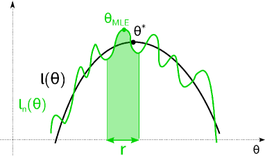
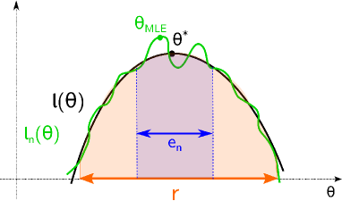
(a)	(b)

Figure 1: (a) A poorly behaved sample likelihood, for which there are many local optima at varying distances from the MLE. It would require an initialization extremely close to the MLE in order to ensure that the Baum-Welch algorithm would not be trapped at a sub-optimal fixed point. (b) A well-behaved sample likelihood, for which all local optima lie within an $e_{n}$-ball of the MLE, as well as the true parameter $\theta^{*}$. In this case, the Baum-Welch algorithm, when initialized within a ball of large radius $r$, will converge to the ball of much smaller radius $e_{n}$. The goal of this paper is to give sufficient conditions for when the sample likelihood exhibits this favorable structure.

Under mild regularity conditions, it is well-known that the maximum likelihood estimate (MLE) for an HMM is a consistent and asymptotically normal estimator; for instance, see Bickel et al. [5], as well as the expository works [17, 18]. On the algorithmic level, the original papers of Baum and co-authors [7, 19] showed that the Baum-Welch algorithm converges to a stationary point of the sample likelihood; these results are in the spirit of the classical convergence analysis of the EM algorithm [20, 8]. These classical convergence results only provide a relatively weak guarantee—namely, that if the algorithm is initialized sufficiently close to the MLE, then it will converge to it. However, the classical analysis does not quantify the size of this neighborhood, and as a critical consequence, it does not rule out the pathological type of behavior illustrated in panel (a) of Figure 1. Here the sample likelihood has multiple optima, both a global optimum corresponding to the MLE as well as many local optima far away from the MLE that are also fixed points of the Baum-Welch algorithm. In such a setting, the Baum-Welch algorithm will only converge to the MLE if it is initialized in an extremely small neighborhood.

In contrast, the goal of this paper is to give sufficient conditions under which the sample likelihood has the more favorable structure shown in panel (b) of Figure 1. Here, even though the MLE does not have a large basin of attraction, the sample likelihood has all of its optima (including the MLE) localized to a small region around the true parameter $\theta^{*}$. Our strategy to reveal this structure, as in our past work [14], is to shift perspective: instead of studying convergence of Baum-Welch updates to the MLE, we study their convergence to an $\epsilon_{n}$-ball of the true parameter $\theta^{*}$, and moreover, instead of focusing exclusively on the sample likelihood, we first study the structure of the population likelihood, corresponding to the idealized limit of infinite data. Our first main result (Theorem 1) provides sufficient conditions under which there is a large ball of radius $r$, over which the population version of the Baum-Welch updates converge at a geometric rate to $\theta^{*}$. Our second main result (Theorem 2) uses empirical process theory to analyze the finite-sample version of the Baum-Welch algorithm, corresponding to what is actually implemented in practice. In this finite sample setting, we guarantee that over the ball of radius $r$, the Baum-Welch updates will converge to an $\epsilon_{n}$-ball with $\epsilon_{n}\ll r$, and most importantly, this $\epsilon_{n}$-ball contains the true parameter $\theta^{*}$. As a side-note, it also contains the MLE, but our theory does not guarantee convergence to the MLE, but rather to a point that is close to both the MLE and the true parameter $\theta^{*}$.

These latter two results are abstract, applicable to a broad class of HMMs. We then specialize them to the case of a hidden Markov mixture consisting of two isotropic components, with means separated by a constant distance, and obtain concrete guarantees for this model. It is worth comparing these results to past work in the i.i.d. setting, for which the problem of Gaussian mixture estimation under various separation assumptions has been extensively studied (e.g., [21, 22, 23, 24]). The constant distance separation required in our work is much weaker than the separation assumptions imposed in papers that focus on correctly labeling samples in a mixture model. Our separation condition is related to, but in general incomparable with the non-degeneracy requirements in other work [11, 25, 24].

Finally, let us discuss the various challenges that arise in studying the dependent data setting of hidden Markov models, and highlight some important differences with the i.i.d. setting [14, 15]. In the non-i.i.d. setting, arguments passing from the population-based to sample-based updates are significantly more delicate. First of all, it is not even obvious that the population version of the $Q$-function—a central object in the Baum-Welch updates—even exists. From a technical standpoint, various gradient smoothness conditions are much more difficult to establish, since the gradient of the likelihood no longer decomposes over the samples as in the i.i.d. setting. In particular, each term in the gradient of the likelihood is a function of all observations. Finally, in order to establish the finite-sample behavior of the Baum-Welch algorithm, we can no longer appeal to standard i.i.d. concentration and empirical process techniques. Nor do we pursue the approach of some past work on HMM estimation (e.g., [11]), in which it is assumed that there are multiple independent samples of the HMM. Instead, we directly analyze the Baum-Welch algorithm that practioners actually use—namely, one that applies to a single sample of an $n$-length HMM. In order to make the argument rigorous, we need to make use of more sophisticated techniques for proving concentration for dependent data [26, 27].

The remainder of this paper is organized as follows. In Section 2, we introduce basic background on hidden Markov models and the Baum-Welch algorithm. Section 3 is devoted to the statement of our main results in the general setting, whereas Section 4 contains the more concrete consequences for the Gaussian output HMM. The main parts of our proofs are given in Section 5, with the more technical details deferred to the appendices.

2 Background and problem set-up

In this section, we introduce some standard background on hidden Markov models and the Baum-Welch algorithm.

2.1 Standard HMM notation and assumptions

We begin by defining a discrete-time hidden Markov model with hidden states taking values in a discrete space. Letting $\mathbb{Z}$ denote the integers, suppose that the observed random variables $\{X_{i}\}_{i\in\mathbb{Z}}$ take values in ^d, and the latent random variables $\{Z_{i}\}_{i\in\mathbb{Z}}$ take values in the discrete space $[s]:\,=\{1,\ldots,s\}$. The Markov structure is imposed on the sequence of latent variables. In particular, if the variable $Z_{1}$ has some initial distribution $\pi_{1}$, then the joint probability of a particular sequence $(z_{1},\ldots,z_{n})$ is given by

$$p(z_{1},\ldots,z_{n};\beta) =\pi_{1}(z_{1};\beta)\prod_{i=1}^{n}p(z_{i}\mid z_{i-1};\beta),$$ (1)

where the vector $\beta$ is a particular parameterization of the initial distribution and Markov chain transition probabilities. We restrict our attention to the homogeneous case, meaning that the transition probabilities for step $(t-1)\rightarrow t$ are independent of the index $t$. Consequently, if we define the transition matrix $A\in^{s\times s}$ with entries

$$A(j,k;\beta):\,=p(z_{2}=k\mid z_{1}=j;\beta),$$

then the marginal distribution $\pi_{i}$ of $Z_{i}$ can be described by the matrix vector equation

$$\pi^{T}_{i} =\pi_{1}^{T}A^{i-1},$$

where $\pi_{i}$ and $\pi_{1}$ denote vectors belonging to the $s$-dimensional probability simplex.

We assume throughout that the Markov chain is aperiodic and recurrent, whence it has a unique stationary distribution $\makebox[0.0pt][l]{\hskip 1.29167pt\rule[5.59721pt]{4.18816pt}{0.43057pt}}{\pi}$, defined by the eigenvector equation $\makebox[0.0pt][l]{\hskip 1.29167pt\rule[5.59721pt]{4.18816pt}{0.43057pt}}{\pi}^{T}=\makebox[0.0pt][l]{\hskip 1.29167pt\rule[5.59721pt]{4.18816pt}{0.43057pt}}{\pi}^{T}A$. To be clear, both $\makebox[0.0pt][l]{\hskip 1.29167pt\rule[5.59721pt]{4.18816pt}{0.43057pt}}{\pi}$ and the matrix $A$ depend on $\beta$, but we omit this dependence so as to simplify notation. We assume throughout that the Markov chain begins in its stationary state, so that $\pi_{1}=\makebox[0.0pt][l]{\hskip 1.29167pt\rule[5.59721pt]{4.18816pt}{0.43057pt}}{\pi}$, and moreover, that it is reversible, meaning that

$$\makebox[0.0pt][l]{\hskip 1.29167pt\rule[5.59721pt]{4.18816pt}{0.43057pt}}{\pi}(j)A(j,k) =\makebox[0.0pt][l]{\hskip 1.29167pt\rule[5.59721pt]{4.18816pt}{0.43057pt}}{\pi}(k)A(k,j)\qquad$$ (2)

for all pairs $j,k\in[s]$.

A key quantity in our analysis is the mixing rate of the Markov chain. In particular, we assume the existence of mixing constant $\epsilon_{\mathrm{mix}}\in(0,1]$ such that

$$\epsilon_{\mathrm{mix}}\leq\frac{p(z_{i}|z_{i-1};\beta)}{\makebox[0.0pt][l]{\hskip 1.29167pt\rule[5.59721pt]{4.18816pt}{0.43057pt}}{\pi}(z_{i})}\leq\epsilon_{\mathrm{mix}}^{-1}$$ (3)

for all $(z_{i},z_{i-1})\in[s]\times[s]$. This condition implies that the dependence on the initial distribution decays geometrically. More precisely, some simple algebra shows that

$$\sup_{\pi_{1}}\left\|\pi_{1}^{T}A^{t}-\pi_{1}^{T}\right\|_{\mathrm{TV}} \leq c_{0}\rho_{\mathrm{mix}}^{t}\qquad\mbox{for all $t=1,2,\ldots$},$$ (4)

where $\rho_{\mathrm{mix}}=1-\epsilon_{\mathrm{mix}}$ denotes the mixing rate of the process, and $c_{0}$ is a universal constant. Note that as $\epsilon_{\mathrm{mix}}\rightarrow 1^{-}$, the Markov chain has behavior approaching that of an i.i.d. sequence, whereas as $\epsilon_{\mathrm{mix}}\rightarrow 0^{+}$, its behavior becomes increasingly “sticky”.

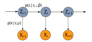
Figure 2: The hidden Markov model as a graphical model. The blue circles indicate observed variables $Z_{i}$, whereas the orange circles indicate latent variables $X_{i}$.

Associated with each latent variable $Z_{i}$ is an observation $X_{i}\in^{d}$. We use $p(x_{i}|z_{i};\mu)$ to denote the density of $X_{i}$ given that $Z_{i}=z_{i}$, an object that we assume to be parameterized by a vector $\mu$. Introducing the shorthand $x_{1}^{n}=(x_{1},\ldots,x_{n})$ and $z_{1}^{n}=(z_{1},\ldots,z_{n})$, the joint probability of the sequence $(x_{1}^{n},z_{1}^{n})$ (also known as the complete likelihood) can be written in the form

$$p(z_{1}^{n},x_{1}^{n};\theta) =\pi_{1}(z_{1})\prod_{i=2}^{n}p(z_{i}\mid z_{i-1};\beta)\prod_{i=1}^{n}p(x_{i}|z_{i};\mu),$$ (5)

where the pair $\theta:\,=(\beta,\mu)$ parameterizes the transition and observation functions. Similarly we define the likelihood

$$p(x_{1}^{n};\theta)=\sum_{z_{1}^{n}}p(z_{1}^{n},x_{1}^{n};\theta).$$

We define a form of complete likelihood 

$$p(z_{0}^{n},x_{1}^{n};\theta) =\pi_{0}(z_{0})\prod_{i=1}^{n}p(z_{i}\mid z_{i-1};\beta)\prod_{i=1}^{n}p(x_{i}|z_{i};\mu),$$ (6)

where $\pi_{0}=\makebox[0.0pt][l]{\hskip 1.29167pt\rule[5.59721pt]{4.18816pt}{0.43057pt}}{\pi}$.

A simple example: A special case helps to illustrate these definitions. In particular, suppose that we have a Markov chain with $s=2$ states. Consider a matrix of transition probabilities $A\in^{2\times 2}$ of the form

$$A =\frac{1}{e^{\beta}+e^{-\beta}}\;\begin{bmatrix}e^{\beta}&e^{-\beta}\\ e^{-\beta}&e^{\beta}\end{bmatrix}\;=\;\begin{bmatrix}\zeta&1-\zeta\\ 1-\zeta&\zeta\end{bmatrix},$$ (7)

where $\zeta:\,=\frac{e^{\beta}}{e^{\beta}+e^{-\beta}}$. By construction, this Markov chain is recurrent and aperiodic with the unique stationary distribution $\makebox[0.0pt][l]{\hskip 1.29167pt\rule[5.59721pt]{4.18816pt}{0.43057pt}}{\pi}=\begin{bmatrix}\frac{1}{2}&\frac{1}{2}\end{bmatrix}^{T}$. Moreover, by calculating the eigenvalues of the transition matrix, we find that the mixing condition (4) holds with $\rho_{\mathrm{mix}}:=|2\zeta-1|=|\tanh(\beta)|$.

Suppose moreover that the observed variables in $\mathbb{R}^{d}$ are conditionally Gaussian, say with

$$p(x_{t}|z_{t};\mu) =\begin{cases}\frac{1}{(2\pi\sigma^{2})^{d/2}}\exp\big{\{}-\frac{1}{2\sigma^{2}}\|x-\mu\|_{2}^{2}\big{\}}&\mbox{if $z_{t}=1$}\\ \frac{1}{(2\pi\sigma^{2})^{d/2}}\exp\big{\{}-\frac{1}{2\sigma^{2}}\|x+\mu\|_{2}^{2}\big{\}}&\mbox{if $z_{t}=2$.}\end{cases}$$ (8)

With this choice, the marginal distribution of each $X_{t}$ is a two-state Gaussian mixture with mean vectors $\mu$ and $-\mu$, and covariance matrices $\sigma^{2}I_{d}$. We provide specific consequences of our general theory for this special case in the sequel.

2.2 Baum-Welch updates for HMMs

We now describe the Baum-Welch updates for a general discrete-state hidden Markov model. As a special case of the EM algorithm, the Baum-Welch algorithm is guaranteed to ascend on the likelihood function of the hidden Markov model. It does so indirectly, by first computing a lower bound on the likelihood (E-step) and then maximizing this lower bound (M-step).

For a given integer $n\geq 1$, suppose that we observe a sequence $x_{1}^{n}=(x_{1},\ldots,x_{n})$ drawn from the marginal distribution over $X_{1}^{n}$ defined by the model (5). The rescaled log likelihood of the sample path $x_{1}^{n}$ is given by

$$\ell_{n}(\theta) =\frac{1}{n}\log\Big{(}\sum_{z_{0}^{n}}p(z_{0}^{n},x_{1}^{n};\theta)\Big{)}$$

The EM likelihood is based on lower bounding the likelihood via Jensen’s inequality. For any choice of parameter $\theta^{\prime}$ and positive integers $i\leq j$ and $a<b$, let $\mathbb{E}_{Z_{i}^{j}|x_{a}^{b},\theta^{\prime}}$ denote the expectation under the conditional distribution $p(Z_{i}^{j}\mid x_{a}^{b};\theta^{\prime})$. With this notation, the concavity of the logarithm and Jensen’s inequality implies that for any choice of $\theta^{\prime}$, we have the lower bound

$$\ell_{n}(\theta) \geq\underbrace{\frac{1}{n}\mathbb{E}_{Z_{0}^{n}|x_{1}^{n},\theta^{\prime}}\big{[}\log p(Z_{0}^{n},x_{1}^{n};\theta)\big{]}}_{Q_{n}(\theta\,\mid\theta^{\prime})}+\underbrace{\frac{1}{n}\mathbb{E}_{Z_{0}^{n}|x_{1}^{n},\theta^{\prime}}\big{[}-\log p(Z_{0}^{n}\mid x_{1}^{n};\theta^{\prime})]}_{H_{n}(\theta^{\prime})}.$$ (9)

For a given choice of $\theta^{\prime}$, the E-step corresponds to the computation of the function $\theta\mapsto Q_{n}(\theta\,\mid\theta^{\prime})$. The $M$-step is defined by the EM operator $M_{n}:\Omega\mapsto\Omega$

$$M_{n}(\theta^{\prime}) =\arg\max_{\theta\in\Omega}Q_{n}(\theta\,\mid\theta^{\prime}),$$ (10)

where $\Omega$ is the set of feasible parameter vectors. Overall, given an initial vector $\theta^{0}=(\beta^{0},\mu^{0})$, the EM algorithm generates a sequence $\{\theta^{t}\}_{t=0}^{\infty}$ according to the recursion $\theta^{t+1}=M_{n}(\theta^{t})$.

This description can be made more concrete for an HMM, in which case the $Q$-function takes the form

$$Q_{n}(\theta\mid\theta^{\prime})=\frac{1}{n}\mathbb{E}_{Z_{0}|x_{1}^{n},\theta^{\prime}}\big{[}\log\pi_{0}(Z_{0};\beta)\big{]}+\frac{1}{n}\sum_{i=1}^{n}\mathbb{E}_{Z_{i-1},Z_{i}|x_{1}^{n},\theta^{\prime}}\big{[}\log p(Z_{i}\mid Z_{i-1};\beta)\big{]}\\ +\frac{1}{n}\sum_{i=1}^{n}{\mathbb{E}}_{Z_{i}\mid x_{1}^{n},\theta^{\prime}}\big{[}\log p(x_{i}\mid Z_{i};\mu)\big{]},$$ (11)

where the dependence of $\pi_{0}$ on $\beta$ comes from the assumption that $\pi_{0}=\makebox[0.0pt][l]{\hskip 1.29167pt\rule[5.59721pt]{4.18816pt}{0.43057pt}}{\pi}$. Note that the $Q$-function can be decomposed as the sum of a term which is solely dependent on $\mu$, and another one which only depends on $\beta$—that is

$$Q_{n}(\theta\mid\theta^{\prime})=Q_{1,n}(\mu\mid\theta^{\prime})+Q_{2,n}(\beta\mid\theta^{\prime})$$ (12)

where $Q_{1,n}(\mu\mid\theta^{\prime})=\frac{1}{n}\sum_{i=1}^{n}{\mathbb{E}}_{Z_{i}\mid x_{1}^{n},\theta^{\prime}}\big{[}\log p(x_{i}\mid Z_{i},\mu)\big{]}$, and $Q_{2,n}(\beta\mid\theta^{\prime})$ collects the remaining terms. In order to compute the expectations defining this function (E-step), we need to determine the marginal distributions over the singletons $Z_{i}$ and pairs $(Z_{i},Z_{i+1})$ under the joint distribution $p(Z_{0}^{n}\mid x_{1}^{n};\theta^{\prime})$. These marginals can be obtained efficiently using a recursive message-passing algorithm, known either as the forward-backward or sum-product algorithm [28, 29].

In the $M$-step, the decomposition (12) suggests that the maximization over the two components $(\beta,\mu)$ can also be decoupled. Accordingly, with a slight abuse of notation, we often write

$$\quad M_{n}^{\mu}(\theta^{\prime})=\arg\max_{\mu\in\Omega_{\mu}}Q_{1,n}(\mu\mid\theta^{\prime}),\quad\mbox{and }\quad M_{n}^{\beta}(\theta^{\prime})=\arg\max_{\beta\in\Omega_{\beta}}Q_{2,n}(\beta\mid\theta^{\prime})$$

for these two decoupled maximization steps, where $\Omega_{\beta}$ and $\Omega_{\mu}$ denote the feasible set of transition and observation parameters respectively and $\Omega:\,=\Omega_{\beta}\times\Omega_{\mu}$.

3 Main results

We now turn to a statement of our main results, along with a discussion of some of their consequences. The first step is to establish the existence of an appropriate population analog of the $Q$-function. Although the existence of such an object is a straightforward consequence of the law of large numbers in the case of i.i.d. data, it requires some technical effort to establish existence for the case of dependent data; in particular, we do so using $k$-truncated version of the full $Q$-function (see Proposition 1). This truncated object plays a central role in the remainder of our analysis. In particular, we first analyze a version of the Baum-Welch updates on the expected $k$-truncated $Q$-function for an extended sequence of observations $x_{1-k}^{n+k}$, and provide sufficient conditions for these population-level updates to be contractive (see Theorem 1). We then use non-asymptotic forms of empirical process theory to show that under suitable conditions, the actual sample-based EM updates—i.e., the updates that are actually implemented in practice—are also well-behaved in this region with high probability (see Theorem 2). In subsequent analysis to follow in Section 4, we show that this initialization radius is suitably large for an HMM with Gaussian outputs.

3.1 Existence of population $Q$-function

In the analysis of Balakrishnan et al. [14], the central object is the notion of a population $Q$-function—namely, the function that underlies the EM algorithm in the idealized limit of infinite data. In their setting of i.i.d. data, the standard law of large numbers ensures that as the sample size $n$ increases, the sample-based $Q$-function approaches its expectation, namely the function

$$\makebox[0.0pt][l]{\hskip 2.05pt\hskip 0.58333pt\rule[8.12498pt]{5.00858pt}{0.43057pt}}{Q}(\theta\mid\theta^{\prime}) =\mathbb{E}\big{[}Q_{n}(\theta\mid\theta^{\prime})\big{]}\;=\;\mathbb{E}\big{[}\mathbb{E}_{Z_{1}|X_{1},\theta^{\prime}}\big{[}\log p(X_{1},Z_{1};\theta)\big{]}\big{]}.$$

Here we use the shorthand $\mathbb{E}$ for the expectation over all samples $X$ that are drawn from the joint distribution (in this case $\mathbb{E}:=\mathbb{E}_{X_{1}^{n}\mid\theta^{*}}$).

When the samples are dependent, the quantity $\mathbb{E}\big{[}Q_{n}(\theta\mid\theta^{\prime})\big{]}$ is no longer independent of $n$, and so an additional step is required. A reasonable candidate for a general definition of the population $Q$-function is given by

$$\makebox[0.0pt][l]{\hskip 2.05pt\hskip 0.58333pt\rule[8.12498pt]{5.00858pt}{0.43057pt}}{Q}(\theta\mid\theta^{\prime}) :\,=\lim_{n\rightarrow+\infty}[\mathbb{E}Q_{n}(\theta\mid\theta^{\prime})].$$ (13)

Although it is clear that this definition is sensible in the i.i.d. case, it is necessary for dependent sampling schemes to prove that the limit given in definition (13) actually exists.

In this paper, we do so by considering a suitably truncated version of the sample-based $Q$-function. Similar arguments have been used in past work (e.g., [17, 18]) to establish consistency of the MLE; here our focus is instead the behavior of the Baum-Welch algorithm. Let us consider a sequence $\{(X_{i},Z_{i})\}_{i=1-k}^{n+k}$, assumed to be drawn from the stationary distribution of the overall chain. Recall that ${\mathbb{E}}_{Z_{i}^{j}\mid x_{a}^{b},\theta}$ denotes expectations taken over the distribution $p(Z_{i}^{j}\mid x_{a}^{b},\theta)$. Then, for a positive integer $k$ to be chosen, we define

$$Q^{k}_{n}(\theta\mid\theta^{\prime})=\frac{1}{n}\Big{[}{\mathbb{E}}_{Z_{0}\mid x_{-k}^{k},\theta^{\prime}}\log p(Z_{1};\beta)+\sum_{i=1}^{n}{\mathbb{E}}_{Z_{i-1}^{i}\mid x_{i-k}^{i+k},\theta^{\prime}}\log p(Z_{i}\mid Z_{i-1};\beta)\\ +\sum_{i=1}^{n}{\mathbb{E}}_{Z_{i}\mid x_{i-k}^{i+k},\theta^{\prime}}\log p(x_{i}\mid Z_{i};\mu)\Big{]}.$$ (14)

In an analogous fashion to the decomposition in equation (11), we can decompose $Q^{k}_{n}$ in the form

$$Q^{k}_{n}(\theta\mid\theta^{\prime})=Q_{1,n}^{k}(\mu\mid\theta^{\prime})+Q_{2,n}^{k}(\beta\mid\theta^{\prime}).$$

We associate with this triplet of $Q$-functions the corresponding EM operators $M^{k}_{n}(\theta^{\prime})$, $M_{n}^{\mu,k}(\theta^{\prime})$ and $M_{n}^{\beta,k}(\theta^{\prime})$ as in Equation (10). Note that as opposed to the function $Q_{n}$ from equation (11), the definition of $Q^{k}_{n}$ involves variables $Z_{i},Z_{i-1}$ that are not conditioned on the full observation sequence $x_{1}^{n}$, but instead only on a $2k$ window centered around the index $i$. By construction, we are guaranteed that the $k$-truncated population function and its decomposed analogs given by

$$\makebox[0.0pt][l]{\hskip 2.05pt\hskip 0.58333pt\rule[8.12498pt]{5.00858pt}{0.43057pt}}{Q}^{k}(\theta\mid\theta^{\prime}) :=\lim_{n\to\infty}\mathbb{E}Q^{k}_{n}(\theta\mid\theta^{\prime})=\mathbb{E}Q_{1,n}^{k}(\mu\mid\theta^{\prime})+\lim_{n\to\infty}\mathbb{E}Q_{2,n}^{k}(\beta\mid\theta^{\prime})$$

$$:=\makebox[0.0pt][l]{\hskip 2.05pt\hskip 0.58333pt\rule[8.12498pt]{5.00858pt}{0.43057pt}}{Q}_{1}^{k}(\mu\mid\theta^{\prime})+\makebox[0.0pt][l]{\hskip 2.05pt\hskip 0.58333pt\rule[8.12498pt]{5.00858pt}{0.43057pt}}{Q}_{2}^{k}(\beta\mid\theta^{\prime})$$ (15)

are well-defined. In particular, due to stationarity of the random sequences $\{p(z_{i}\mid X_{i-k}^{i+k})\}_{i=1}^{n}$ and $\{p(z_{i-1}^{i}\mid X_{i-k}^{i+k})\}_{i=1}^{n}$, the expectation over $\{(X_{i},Z_{i})\}_{i=1-k}^{n+k}$ is independent of the sample size $n$.

Our first result uses the existence of this truncated population object in order to show that the standard population $Q$-function from equation (13) is indeed well-defined. In doing so, we make use of the sup-norm

$$\|Q_{1}-Q_{2}\|_{\infty} :\,=\sup_{\theta,\theta^{\prime}\in\Omega}\Big{|}Q_{1}(\theta\mid\theta^{\prime})-Q_{2}(\theta\mid\theta^{\prime})\Big{|}.$$ (16)

For a radius $r>0$, define the ball $\mathbb{B}_{2}(r;\mu^{*})=\{\mu\in^{d}\,\mid\,\|\mu-\mu^{*}\|_{2}\leq r\}$. We require in the following that the observation densities satisfy the following boundedness condition

$$\sup_{\theta\in\mathbb{B}_{2}(r;\theta^{*})}{\mathbb{E}}\Big{[}\max_{z_{i}\in[s]}\big{|}\log p(X_{i}|z_{i};\mu)\big{|}\Big{]}<\infty.$$ (17)

Proposition 1.

Under the previously stated assumptions, the population function $\makebox[0.0pt][l]{\hskip 2.05pt\hskip 0.58333pt\rule[8.12498pt]{5.00858pt}{0.43057pt}}{Q}$ defined in equation (13) exists.

The proof of this claim is given in Appendix A. It hinges on the following auxiliary claim, which bounds the difference between $\mathbb{E}Q_{n}$ and the $k$-truncated $Q$-function as

$$\|\mathbb{E}Q_{n}-\makebox[0.0pt][l]{\hskip 2.05pt\hskip 0.58333pt\rule[8.12498pt]{5.00858pt}{0.43057pt}}{Q}^{k}\|_{\infty} \leq\frac{c\,s^{5}}{\epsilon_{\mathrm{mix}}^{8}\makebox[0.0pt][l]{\hskip 1.29167pt\rule[5.59721pt]{4.18816pt}{0.43057pt}}{\pi}_{\min}^{2}}\big{(}1-\epsilon_{\mathrm{mix}}\makebox[0.0pt][l]{\hskip 1.29167pt\rule[5.59721pt]{4.18816pt}{0.43057pt}}{\pi}_{\min}\big{)}^{k}+\frac{1}{n}\log\makebox[0.0pt][l]{\hskip 1.29167pt\rule[5.59721pt]{4.18816pt}{0.43057pt}}{\pi}_{\min}^{-1},$$ (18)

where $\makebox[0.0pt][l]{\hskip 1.29167pt\rule[5.59721pt]{4.18816pt}{0.43057pt}}{\pi}_{\min}:=\min_{\beta\in\Omega_{\beta},j\in[s]}\makebox[0.0pt][l]{\hskip 1.29167pt\rule[5.59721pt]{4.18816pt}{0.43057pt}}{\pi}(j\mid\beta)$ is the minimum probability in the stationary distribution, and $\epsilon_{\mathrm{mix}}$ is the mixing constant from equation (3). Note that the dependencies on $\epsilon_{\mathrm{mix}}$ and $\makebox[0.0pt][l]{\hskip 1.29167pt\rule[5.59721pt]{4.18816pt}{0.43057pt}}{\pi}_{\min}$ are not optimized here since it would not help to illustrate the main ideas more clearly. Since this bound holds for all $n$, it shows that the population function $\makebox[0.0pt][l]{\hskip 2.05pt\hskip 0.58333pt\rule[8.12498pt]{5.00858pt}{0.43057pt}}{Q}$ can be uniformly approximated by $\makebox[0.0pt][l]{\hskip 2.05pt\hskip 0.58333pt\rule[8.12498pt]{5.00858pt}{0.43057pt}}{Q}^{k}$, with the approximation error decreasing geometrically as the truncation level $k$ grows. This fact plays an important role in the analysis to follow.

3.2 Analysis of updates based on $\makebox[0.0pt][l]{\hskip 2.05pt\hskip 0.58333pt\rule[8.12498pt]{5.00858pt}{0.43057pt}}{Q}^{k}$

Our ultimate goal is to establish a bound on the difference between the sample-based Baum-Welch estimate and $\theta^{*}$, in particular showing contraction of the Baum-Welch update towards the true parameter. Our strategy for doing so involves first analyzing the Baum-Welch iterates at the population level, which is the focus of this section.

The quantity $\makebox[0.0pt][l]{\hskip 2.05pt\hskip 0.58333pt\rule[8.12498pt]{5.00858pt}{0.43057pt}}{Q}$ is significant for the EM updates because the parameter $\theta^{*}$ satisfies the self-consistency property $\theta^{*}=\operatorname*{arg\,max}_{\theta}\makebox[0.0pt][l]{\hskip 2.05pt\hskip 0.58333pt\rule[8.12498pt]{5.00858pt}{0.43057pt}}{Q}(\theta\mid\theta^{*})$. In the i.i.d. setting, the function $\makebox[0.0pt][l]{\hskip 2.05pt\hskip 0.58333pt\rule[8.12498pt]{5.00858pt}{0.43057pt}}{Q}$ can often be computed in closed form, and hence directly analyzed, as was done in past work [14]. In the HMM case, this function $\makebox[0.0pt][l]{\hskip 2.05pt\hskip 0.58333pt\rule[8.12498pt]{5.00858pt}{0.43057pt}}{Q}$ no longer has a closed form, so an alternative route is needed. Here we analyze the population version via the truncated function $\makebox[0.0pt][l]{\hskip 2.05pt\hskip 0.58333pt\rule[8.12498pt]{5.00858pt}{0.43057pt}}{Q}^{k}$ (15) instead, where $k$ is a given truncation level (to be chosen in the sequel). Although $\theta^{*}$ is no longer a fixed point of $\makebox[0.0pt][l]{\hskip 2.05pt\hskip 0.58333pt\rule[8.12498pt]{5.00858pt}{0.43057pt}}{Q}^{k}$, the bound (18) combined with the assumption of strong concavity of $\makebox[0.0pt][l]{\hskip 2.05pt\hskip 0.58333pt\rule[8.12498pt]{5.00858pt}{0.43057pt}}{Q}^{k}$ imply an upper bound on the distance of the maximizers of $\makebox[0.0pt][l]{\hskip 2.05pt\hskip 0.58333pt\rule[8.12498pt]{5.00858pt}{0.43057pt}}{Q}^{k}$ and $\makebox[0.0pt][l]{\hskip 2.05pt\hskip 0.58333pt\rule[8.12498pt]{5.00858pt}{0.43057pt}}{Q}$.

With this setup, we consider an idealized population-level algorithm that, based on some initialization $\widetilde{\theta}^{0}\in\Omega=\mathbb{B}_{2}\big{(}r;\mu^{*}\big{)}\times\Omega_{\beta}$, generates the sequence of iterates

$$\widetilde{\theta}^{t+1}=\makebox[0.0pt][l]{\hskip 2.05pt\rule[8.12498pt]{8.30453pt}{0.43057pt}}{M}^{k}(\widetilde{\theta}^{t}):=\operatorname*{arg\,max}_{\theta\in\Omega}\makebox[0.0pt][l]{\hskip 2.05pt\hskip 0.58333pt\rule[8.12498pt]{5.00858pt}{0.43057pt}}{Q}^{k}(\theta\mid\widetilde{\theta}^{t}).$$ (19)

Since $\makebox[0.0pt][l]{\hskip 2.05pt\hskip 0.58333pt\rule[8.12498pt]{5.00858pt}{0.43057pt}}{Q}^{k}$ is an approximate version of $\makebox[0.0pt][l]{\hskip 2.05pt\hskip 0.58333pt\rule[8.12498pt]{5.00858pt}{0.43057pt}}{Q}$, the update operator $\makebox[0.0pt][l]{\hskip 2.05pt\rule[8.12498pt]{8.30453pt}{0.43057pt}}{M}^{k}$ should be understood as an approximation to the idealized population EM operator $\makebox[0.0pt][l]{\hskip 2.05pt\rule[8.12498pt]{8.30453pt}{0.43057pt}}{M}$ where the maximum is taken with respect to $\makebox[0.0pt][l]{\hskip 2.05pt\hskip 0.58333pt\rule[8.12498pt]{5.00858pt}{0.43057pt}}{Q}$. As part (a) of the following theorem shows, the approximation error is well-controlled under suitable conditions. We analyze the convergence of the sequence $\{\widetilde{\theta}^{t}\}_{t=0}^{\infty}$ in terms of the norm $\|\cdot\|_{\star}:\Omega_{\mu}\times\Omega_{\beta}\to\mathbb{R}^{+}$ given by

$$\|\theta-\theta^{*}\|_{\star}=\|(\mu,\beta)-(\mu^{*},\beta^{*})\|_{\star}:\,=\|\mu-\mu^{*}\|_{2}+\|\beta-\beta^{*}\|_{2}.$$ (20)

Contraction in this norm implies that both parameters $\mu,\beta$ converge linearly to the true parameter.

Conditions on $\makebox[0.0pt][l]{\hskip 2.05pt\hskip 0.58333pt\rule[8.12498pt]{5.00858pt}{0.43057pt}}{Q}^{k}$:

Let us now introduce the conditions on the truncated function $\makebox[0.0pt][l]{\hskip 2.05pt\hskip 0.58333pt\rule[8.12498pt]{5.00858pt}{0.43057pt}}{Q}^{k}$ that underlie our analysis. For a radius $r>0$, we concentrate on showing conditions in the Cartesian product

$$\Omega :\,=\mathbb{B}_{2}(r;\mu^{*})\times\Omega_{\beta},$$

where $\Omega_{\beta}$ is the set of allowable HMM transition parameters. First, let us say that the function $\makebox[0.0pt][l]{\hskip 2.05pt\hskip 0.58333pt\rule[8.12498pt]{5.00858pt}{0.43057pt}}{Q}^{k}(\cdot\mid\theta^{\prime})$ is $(\lambda_{\mu},\lambda_{\beta})$-strongly concave in $\Omega$ if

$$\makebox[0.0pt][l]{\hskip 2.05pt\hskip 0.58333pt\rule[8.12498pt]{5.00858pt}{0.43057pt}}{Q}_{1}^{k}(\mu_{1}\mid\theta^{*})-\makebox[0.0pt][l]{\hskip 2.05pt\hskip 0.58333pt\rule[8.12498pt]{5.00858pt}{0.43057pt}}{Q}_{1}^{k}(\mu_{2}\mid\theta^{*})-\langle\nabla_{\mu}\makebox[0.0pt][l]{\hskip 2.05pt\hskip 0.58333pt\rule[8.12498pt]{5.00858pt}{0.43057pt}}{Q}_{1}^{k}(\mu_{2}\mid\theta^{*}),\mu_{1}-\mu_{2}\rangle \leq-\frac{\lambda_{\mu}}{2}\|\mu_{1}-\mu_{2}\|_{2}^{2}$$ (21a)

$$\mbox{and}\qquad\makebox[0.0pt][l]{\hskip 2.05pt\hskip 0.58333pt\rule[8.12498pt]{5.00858pt}{0.43057pt}}{Q}_{2}^{k}(\beta_{1}\mid\theta^{*})-\makebox[0.0pt][l]{\hskip 2.05pt\hskip 0.58333pt\rule[8.12498pt]{5.00858pt}{0.43057pt}}{Q}_{2}^{k}(\beta_{2}\mid\theta^{*})-\langle\nabla_{\beta}\makebox[0.0pt][l]{\hskip 2.05pt\hskip 0.58333pt\rule[8.12498pt]{5.00858pt}{0.43057pt}}{Q}_{2}^{k}(\beta_{2}\mid\theta^{*}),\beta_{1}-\beta_{2}\rangle \leq-\frac{\lambda_{\beta}}{2}\|\beta_{1}-\beta_{2}\|_{2}^{2}$$ (21b)

for all $(\mu_{1},\beta_{1}),(\mu_{2},\beta_{2})\in\Omega$.

Second, we impose first-order stability conditions on the gradients of each component of $\makebox[0.0pt][l]{\hskip 2.05pt\hskip 0.58333pt\rule[8.12498pt]{5.00858pt}{0.43057pt}}{Q}^{k}$:

• For each $\mu\in\Omega_{\mu},\theta^{\prime}\in\Omega$, we have

  $$\|\nabla_{\mu}\makebox[0.0pt][l]{\hskip 2.05pt\hskip 0.58333pt\rule[8.12498pt]{5.00858pt}{0.43057pt}}{Q}_{1}^{k}(\mu\mid\mu^{\prime},\beta^{\prime})-\nabla_{\mu}\makebox[0.0pt][l]{\hskip 2.05pt\hskip 0.58333pt\rule[8.12498pt]{5.00858pt}{0.43057pt}}{Q}_{1}^{k}(\mu\mid\mu^{*},\beta^{\prime})\|_{2} \leq L_{\mu,1}\|\mu^{\prime}-\mu^{*}\|_{2}$$ (22a)

  $$\|\nabla_{\mu}\makebox[0.0pt][l]{\hskip 2.05pt\hskip 0.58333pt\rule[8.12498pt]{5.00858pt}{0.43057pt}}{Q}_{1}^{k}(\mu\mid\mu^{\prime},\beta^{\prime})-\nabla_{\mu}\makebox[0.0pt][l]{\hskip 2.05pt\hskip 0.58333pt\rule[8.12498pt]{5.00858pt}{0.43057pt}}{Q}_{1}^{k}(\mu\mid\mu^{\prime},\beta^{*})\|_{2} \leq L_{\mu,2}\|\beta^{\prime}-\beta^{*}\|_{2},$$ (22b)

  We refer to this condition as $L_{\mu}$-FOS for short.

• Secondly, for all $\beta\in\Omega_{\beta},\theta^{\prime}\in\Omega$, we require that

  $$\|\nabla_{\beta}\makebox[0.0pt][l]{\hskip 2.05pt\hskip 0.58333pt\rule[8.12498pt]{5.00858pt}{0.43057pt}}{Q}_{2}^{k}(\beta\mid\mu^{\prime},\beta^{\prime})-\nabla_{\beta}\makebox[0.0pt][l]{\hskip 2.05pt\hskip 0.58333pt\rule[8.12498pt]{5.00858pt}{0.43057pt}}{Q}_{2}^{k}(\beta\mid\mu^{*},\beta^{\prime})\|_{2} \leq L_{\beta,1}\|\mu^{\prime}-\mu^{*}\|_{2}$$ (23a)

  $$\|\nabla_{\beta}\makebox[0.0pt][l]{\hskip 2.05pt\hskip 0.58333pt\rule[8.12498pt]{5.00858pt}{0.43057pt}}{Q}_{2}^{k}(\beta\mid\mu^{\prime},\beta^{\prime})-\nabla_{\beta}\makebox[0.0pt][l]{\hskip 2.05pt\hskip 0.58333pt\rule[8.12498pt]{5.00858pt}{0.43057pt}}{Q}_{2}^{k}(\beta\mid\mu^{\prime},\beta^{*})\|_{2} \leq L_{\beta,2}\|\beta^{\prime}-\beta^{*}\|_{2}.$$ (23b)

  We refer to this condition as $L_{\beta}$-FOS for short.

As we show in Section 4, these conditions hold for concrete models.

Convergence guarantee for $\makebox[0.0pt][l]{\hskip 2.05pt\hskip 0.58333pt\rule[8.12498pt]{5.00858pt}{0.43057pt}}{Q}^{k}$-updates:

We are now equipped to state our main convergence guarantee for the updates. It involves the quantities

$$L:\,=\max\{L_{\mu_{1}},L_{\mu_{2}}\}+\max\{L_{\beta_{1}},L_{\beta_{2}}\},\quad\lambda:\,=\min\{\lambda_{\mu},\lambda_{\beta}\}\quad\mbox{and }\quad\kappa:\,=\frac{L}{\lambda},$$ (24)

with $\kappa$ generally required to be smaller than one, as well as the additive norm $\|\cdot\|_{\star}$ from equation (20).

Part (a) of the theorem controls the approximation error induced by using the $k$-truncated function $\makebox[0.0pt][l]{\hskip 2.05pt\hskip 0.58333pt\rule[8.12498pt]{5.00858pt}{0.43057pt}}{Q}^{k}$ as opposed to the exact population function $\makebox[0.0pt][l]{\hskip 2.05pt\hskip 0.58333pt\rule[8.12498pt]{5.00858pt}{0.43057pt}}{Q}$, whereas part (b) guarantees a geometric rate of convergence in terms of $\kappa$ defined above in equation (24).

Theorem 1.

1. Approximation guarantee: Under the mixing condition (4), density boundedness condition (17), and $(\lambda_{\mu},\lambda_{\beta})$-strong concavity condition (21), there is a universal constant $c_{0}$ such that

   $$\|\makebox[0.0pt][l]{\hskip 2.05pt\rule[8.12498pt]{8.30453pt}{0.43057pt}}{M}^{k}(\theta)-\makebox[0.0pt][l]{\hskip 2.05pt\rule[8.12498pt]{8.30453pt}{0.43057pt}}{M}(\theta)\|_{\star}^{2} \leq\underbrace{c_{0}\frac{s^{5}}{\lambda\,\epsilon_{\mathrm{mix}}^{8}\makebox[0.0pt][l]{\hskip 1.29167pt\rule[5.59721pt]{4.18816pt}{0.43057pt}}{\pi}_{\min}^{2}}\big{(}1-\epsilon_{\mathrm{mix}}\makebox[0.0pt][l]{\hskip 1.29167pt\rule[5.59721pt]{4.18816pt}{0.43057pt}}{\pi}_{\min}\big{)}^{k}}_{=:\varphi^{2}(k)}\qquad\mbox{for all $\theta\in\Omega$,}$$ (25)

   where $s$ is the number of states, and $\makebox[0.0pt][l]{\hskip 1.29167pt\rule[5.59721pt]{4.18816pt}{0.43057pt}}{\pi}_{\min}:\,=\min\limits_{\beta\in\Omega_{\beta}}\min\limits_{j\in[s]}\makebox[0.0pt][l]{\hskip 1.29167pt\rule[5.59721pt]{4.18816pt}{0.43057pt}}{\pi}(j;\beta)$.

2. Convergence guarantee: Suppose in addition that the $(L_{\mu},L_{\beta})$-FOS conditions (22),(23) holds with parameter $\kappa\in(0,1)$ as defined in (24) for $\theta,\theta^{\prime}\in\Omega=\mathbb{B}_{2}\big{(}r;\mu^{*}\big{)}\times\Omega_{\beta}$, and that the truncation parameter $k$ is sufficiently large to ensure that

   $$\varphi(k)\leq\big{(}1-\kappa\big{)}r-\kappa\max_{\beta\in\Omega_{\beta}}\|\beta-\beta^{*}\|_{2}.$$

   Then given an initialization $\widetilde{\theta}^{0}\in\Omega$, the iterates $\{\widetilde{\theta}^{t}\}_{t=0}^{\infty}$ generated by the $\makebox[0.0pt][l]{\hskip 2.05pt\rule[8.12498pt]{8.30453pt}{0.43057pt}}{M}^{k}$ operator satisfy the bound

   $$\|\widetilde{\theta}^{t}-\theta^{*}\|_{\star} \leq\kappa^{t}\|\widetilde{\theta}^{0}-\theta^{*}\|_{\star}+\frac{1}{1-\kappa}\varphi(k).$$ (26)

Note that the subtlety here is that $\theta^{*}$ is no longer a fixed point of the operator $\makebox[0.0pt][l]{\hskip 2.05pt\rule[8.12498pt]{8.30453pt}{0.43057pt}}{M}^{k}$, due to the error induced by the $k^{th}$-order truncation. Nonetheless, under a mixing condition, as the bounds (25) and (26) show, this approximation error is controlled, and decays exponentially in $k$. The proof of the recursive bound (26) is based on first showing that

$$\|\makebox[0.0pt][l]{\hskip 2.05pt\rule[8.12498pt]{8.30453pt}{0.43057pt}}{M}^{k}(\theta)-\makebox[0.0pt][l]{\hskip 2.05pt\rule[8.12498pt]{8.30453pt}{0.43057pt}}{M}^{k}(\theta^{*})\|_{\star} \leq\kappa\|\theta-\theta^{*}\|_{\star}$$ (27)

for any $\theta\in\Omega$. Inequality (27) is equivalent to stating that the operator $\makebox[0.0pt][l]{\hskip 2.05pt\rule[8.12498pt]{8.30453pt}{0.43057pt}}{M}^{k}$ is contractive, i.e. that applying $\makebox[0.0pt][l]{\hskip 2.05pt\rule[8.12498pt]{8.30453pt}{0.43057pt}}{M}^{k}$ to the pair $\theta$ and $\theta^{*}$ always decreases the distance.

Finally, when Theorem 1 is applied to a concrete model, the task is to find the biggest $r$ and $\Omega_{\beta}$ such that the conditions in the theorem are satisfied, and we do so for the Gaussian output HMM in Section 4.

3.3 Sample-based results

We now turn to a result that applies to the sample-based form of the Baum-Welch algorithm—that is, corresponding to the updates that are actually applied in practice. For a tolerance parameter $\delta\in(0,1)$, we let $\varphi_{n}(\delta,k)$ be the smallest positive scalar such that

$$\sup_{\theta\in\mathbb{B}_{2}(r;\theta^{*})}\mathbb{P}\Big{[}\|M_{n}(\theta)-M^{k}_{n}(\theta)\|_{\star}\geq\varphi_{n}(\delta,k)\Big{]} \leq\delta.$$ (28a)

This quantity bounds the approximation error induced by the $$k \varphi(k) \delta\in(0,1) \epsilon^{\mu}_{n}(\delta,k) \epsilon^{\beta}_{n}(\delta,k)$$-truncation, and is the sample-based analogue of the quantity appearing in Theorem 1(a). For each , we let and denote the smallest positive scalars such that

$$\mathbb{P}\big{[}\|M_{n}^{\mu,k}(\theta)-\makebox[0.0pt][l]{\hskip 2.05pt\rule[8.12498pt]{8.30453pt}{0.43057pt}}{M}^{\mu,k}(\theta)\|_{2}\geq\epsilon^{\mu}_{n}(\delta,k)\Big{]}\leq\delta,\quad\mbox{and}\quad\mathbb{P}\big{[}\|M_{n}^{\beta,k}(\theta)-\makebox[0.0pt][l]{\hskip 2.05pt\rule[8.12498pt]{8.30453pt}{0.43057pt}}{M}^{\beta,k}(\theta)\|_{2}\geq\epsilon^{\beta}_{n}(\delta,k)\Big{]}\leq\delta$$ (28b)

for all $$\theta\in\mathbb{B}_{2}(\mu^{*};r)\times\Omega_{\beta}$$.

Furthermore we define $\epsilon_{n}(\delta,k):\,=\epsilon^{\mu}_{n}(\delta,k)+\epsilon^{\beta}_{n}(\delta,k)$. For a given truncation level $k$, these values give an upper bound on the difference between the population and sample-based $M$-operators, as induced by having only a finite number $n$ of samples.

Theorem 2 (Sample Baum-Welch).

Suppose that the truncated population EM operator $\makebox[0.0pt][l]{\hskip 2.05pt\rule[8.12498pt]{8.30453pt}{0.43057pt}}{M}^{k}$ satisfies the local contraction bound (27) with parameter $\kappa\in(0,1)$ in $\Omega$. For a given sample size $n$, suppose that $(k,n)$ are sufficiently large to ensure that

$$\varphi_{n}(\delta,k)+\epsilon^{\mu}_{n}\big{(}\delta,k\big{)}+\varphi(k) \leq(1-\kappa)\,r-\kappa\max_{\beta\in\Omega_{\beta}}\|\beta-\beta^{*}\|_{2}.$$ (29a)

Then given any initialization $$\widehat{\theta}^{0}\in\Omega 1-2\delta \{\widehat{\theta}^{t}\}_{t=0}^{\infty}$$, with probability at least , the Baum-Welch sequence satisfies the bound

$$\|\widehat{\theta}^{t}-\theta^{*}\|_{\star} \leq\underbrace{\kappa^{t}\|\widehat{\theta}^{0}-\theta^{*}\|_{\star}}_{\mbox{Geometric decay}}+\underbrace{\frac{1}{1-\kappa}\Big{\{}2\varphi_{n}\big{(}\delta,k\big{)}+\epsilon_{n}\big{(}\delta,k\big{)}+\varphi(k)\Big{\}}}_{\mbox{Residual error $e_{n}$}}.$$ (29b)

The bound (29b) shows that the distance between $\widehat{\theta}^{t}$ and $\theta^{*}$ is bounded by two terms: the first decays geometrically as $t$ increases, and the second term corresponds to a residual error term that remains independent of $t$. Thus, by choosing the iteration number $T$ larger than $\frac{\log(2r/\epsilon)}{\log\kappa}$, we can ensure that the first term is at most $\epsilon$. The residual error term can be controlled by requiring that the sample size $n$ is sufficiently large, and then choosing the truncation level $k$ appropriately. We provide a concrete illustration of this procedure in the following section, where we analyze the case of Gaussian output HMMs. In particular, we can see that the residual error is of the same order as for the MLE and that the required initialization radius is optimal up to constants. Let us emphasize here that $k$ as well as the truncated operators are purely theoretical objects which were introduced for the analysis.

4 Concrete results for the Gaussian output HMM

We now return to the concrete example of a Gaussian output HMM, as first introduced in Section 2.1, and specialize our general theory to it. Before doing so, let us make some preliminary comments about our notation and assumptions. Recall that our Gaussian output HMM is based on $s=2$ hidden states, using the transition matrix from equation (7), and the Gaussian output densities from equation (8). For convenience of analysis, we let the hidden variables $Z_{i}$ take values in $\{-1,1\}$. In addition, we require that the mixing coefficient $\rho_{\mathrm{mix}}=1-\epsilon_{\mathrm{mix}}$ is bounded away from $1$ in order to ensure that the mixing condition (3) is fulfilled. We denote the upper bound for $\rho_{\mathrm{mix}}$ as $b<1$ so that $\rho_{\mathrm{mix}}\leq b$ and $\epsilon_{\mathrm{mix}}\geq 1-b$. The feasible set of the probability parameter $\zeta$ and its log odds analog $\beta=\frac{1}{2}\log\big{(}\frac{\zeta}{1-\zeta}\big{)}$ are then given by

$$\Omega_{\zeta}=\left\{\zeta\in\mid\frac{1-b}{2}\leq\zeta\leq\frac{1+b}{2}\right\},\quad\mbox{and}\quad\Omega_{\beta}=\Big{\{}\beta\in\;\mid\;|\beta|<\underbrace{\frac{1}{2}\log\big{(}\frac{1+b}{1-b}\big{)}}_{\beta_{B}}\Big{\}}.$$ (30)

4.1 Explicit form of Baum-Welch updates

We begin by deriving an explicit form of the Baum-Welch updates for this model. Using this notation, the Baum-Welch updates take the form

$$\widehat{\mu}^{t+1} =\frac{1}{n}\sum_{i=1}^{n}(2p(Z_{i}=1\mid x_{1}^{n};\theta^{t})-1)x_{i},$$ (31a)

$$\widehat{\zeta}^{t+1} =\Pi_{\Omega_{\zeta}}\left(\frac{1}{n}\sum_{i=1}^{n}\sum_{Z_{i}}p(Z_{i}=Z_{i+1}\mid x_{1}^{n};\theta^{t})\right),\text{ and }$$ (31b)

$$\widehat{\beta}^{t+1} =\frac{1}{2}\log\big{(}\frac{\widehat{\zeta}^{t+1}}{1-\widehat{\zeta}^{t+1}}\big{)},$$ (31c)

where $\Pi_{\Omega_{\zeta}}$ denotes the Euclidean projection onto the set $\Omega_{\zeta}$. Note that the maximization steps are carried out on the decomposed $Q$-functions $Q_{1,n}(\cdot\mid\theta^{t}),Q_{2,n}(\cdot\mid\theta^{t})$. In addition, since we are dealing with a one-dimensional quantity $\beta$, the projection of the unconstrained maximizer onto the interval $\Omega_{\zeta}$ is equivalent to the constrained maximizer over the feasible set $\Omega_{\zeta}$. This step is in general not valid for higher dimensional transition parameters.

4.2 Population and sample guarantees

We now use the results from Section 3 to show that the population and sample-based version of the Baum-Welch updates are linearly convergent in a ball around $\theta^{*}$ of fixed radius. In establishing the population-level guarantee, the key conditions which need to be fulfilled—and the one that are the most technically challenging to establish— are the $(L_{\mu},L_{\beta})$-FOS conditions (22), (23). In particular, we want to show that these conditions hold with Lipschitz constants $L_{\mu},L_{\beta}$ that decrease exponentially with the separation of the mixtures. As a consequence, we obtain that for large enough separation $\frac{L}{\lambda}<1$, i.e. the EM operator is contractive towards the true parameter.

Throughout this section, we use $c_{0},c_{1}$ to denote universal constants and $C_{0},C_{1}$ for quantities that do not depend on $(\|\mu^{*}\|_{2},\sigma)$, but may depend on other parameters such as $\makebox[0.0pt][l]{\hskip 1.29167pt\rule[5.59721pt]{4.18816pt}{0.43057pt}}{\pi}_{\min}$, $\rho_{\mathrm{mix}}$, $b$, and so on. In order to ease notation, our explicit tracking of parameter dependence is limited to the standard deviation $\sigma$ and Euclidean norm $\|\mu^{*}\|_{2}$, which together determine the signal-to-noise ratio $\eta^{2}:\,=\frac{\|\mu^{*}\|_{2}^{2}}{\sigma^{2}}$ of the mixture model. We use the notation

We begin by stating a result for the sequence $\{\widetilde{\theta}^{t}\}_{t=0}^{\infty}$ obtained by repeatedly applying the $k$-truncated population-level Baum-Welch update operator $\makebox[0.0pt][l]{\hskip 2.05pt\rule[8.12498pt]{8.30453pt}{0.43057pt}}{M}^{k}$. Our first corollary establishes that this sequence is linearly convergent, with a convergence rate $\kappa=\kappa(\eta)$ that is given by

$$\kappa(\eta) :\,=\frac{C_{1}\eta^{2}(\eta^{2}+1)\;\mathrm{e}^{-c_{2}\eta^{2}}}{1-b^{2}}.$$ (32)

Corollary 1 (Population Baum-Welch).

Consider a two-state Gaussian output HMM that is mixing (i.e. satisfies equation (3)), and with its SNR lower bounded as $\eta^{2}\geq C$ for a sufficiently large constant $C$. Given the radius $r=\frac{\|\mu^{*}\|_{2}}{4}$, suppose that the truncation parameter $k$ is sufficiently large to ensure that $\varphi(k)\leq(1-\kappa)r-\kappa\max_{\beta\in\Omega_{\beta}}\|\beta-\beta^{*}\|_{2}$. Then for any initialization $\widetilde{\theta}^{0}=(\widetilde{\mu}^{0},\widetilde{\beta}^{0})\in\mathbb{B}_{2}\big{(}r;\mu^{*}\big{)}\times\Omega_{\beta}$, the sequence $\{\widetilde{\theta}^{t}\}_{t=0}^{\infty}$ generated by $\makebox[0.0pt][l]{\hskip 2.05pt\rule[8.12498pt]{8.30453pt}{0.43057pt}}{M}^{k}$ satisfies the bound

$$\|\widetilde{\theta}^{t}-\theta^{*}\|_{\star} \leq\kappa^{t}\|\widetilde{\theta}^{0}-\theta^{*}\|_{\star}+\frac{1}{1-\kappa}\varphi(k)$$ (33)

for all iterations $t=1,2,\ldots$.

From definition (32) it follows that as long as the signal-to-noise ratio $\eta$ is larger than a universal constant, the convergence rate $\kappa(\eta)<1$. The bound (33) then ensures a type of contraction and the pre-condition $\varphi(k)\leq(1-\kappa)r-\kappa\max_{\beta\in\Omega_{\beta}}\|\beta-\beta^{*}\|_{2}$ can be satisfied by choosing the truncation parameter $k$ large enough. If we use a finite truncation parameter $k$, then the contraction occurs up to the error floor given by $\varphi(k)$, which reflects the bias introduced by truncating the likelihood to a window of size $k$. At the population level (in which the effective sample size is infinite), we could take the limit $k\rightarrow\infty$ so as to eliminate this bias. However, this is no longer possible in the finite sample setting, in which we must necessarily have $k\ll n$.

Corollary 2 (Sample Baum-Welch iterates).

For a given tolerance $\delta\in(0,1)$, suppose that the sample size is lower bounded as $n\geq C_{1}(\sigma^{2}+\|\mu^{*}\|_{2}^{2})d\log^{2}(\frac{d}{\delta})$ for a sufficiently large $C_{1}$. Then under the conditions of Corollary 1, with probability at least $1-\delta$, we have

$$\|\widetilde{\theta}^{t}-\theta^{*}\|_{\star}\leq\kappa^{t}\|\widehat{\theta}^{0}-\theta^{*}\|_{\star}+C\frac{\|\mu^{*}\|_{2}(\frac{\|\mu^{*}\|_{2}^{2}}{\sigma^{2}}+1)\log^{2}n\sqrt{\frac{d\log^{2}(n/\delta)}{n}}}{1-\kappa}.$$ (34)

Remarks:

As a consequence of the bound (34), if we are given a sample size $n\succsim d\log^{2}d$, then taking $T\approx\log n$ iterations is guaranteed to return an estimate $(\widehat{\mu}^{T},\widehat{\beta}^{T})$ with error of the order $\sqrt{\frac{d\log^{6}(n)}{n}}$.

In order to interpret this guarantee, note that in the case of symmetric Gaussian output HMMs as in Section 4, standard techniques can be used to show that the minimax rate of estimating $\mu^{*}$ in Euclidean norm scales as $\sqrt{\frac{d}{n}}$. If we could compute the MLE in polynomial time, then its error would also exhibit this scaling. The significance of Corollary 2 is that it shows that the Baum-Welch update achieves this minimax risk of estimation up to logarithmic factors.

Moreover, it should be noted that the initialization radius given here is essentially optimal up to constants. Because of the symmetric nature of the population log-likelihood, the all zeroes vector is a stationary point. Consequently, the maximum Euclidean radius of any basin of attraction for one of the observation parameters—that is, either $\mu^{*}$ or $-\mu^{*}$—can at most be $r=\|\mu^{*}\|_{2}$. Note that our initialization radius only differs from this maximal radius by only a small constant factor.

4.3 Simulations

In this section, we provide the results of simulations that confirm the accuracy of our theoretical predictions for two-state Gaussian output HMMs. In all cases, we update the estimates for the mean vector $\widehat{\mu}^{t+1}$ and transition probability $\hat{\zeta}^{t+1}$ according to equation (31); for convenience, we update $\zeta$ as opposed to $\beta$. The true parameters are denoted by $\mu^{*}$ and $\zeta^{*}$.

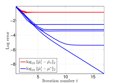
Figure 3: Plot of the convergence of the optimization error $\log\|\widehat{\mu}_{i}^{t}-\widehat{\mu}_{1}\|_{2}$, plotted in blue, and the statistical error $\log\|\widehat{\mu}_{i}^{t}-\mu^{*}\|_{2}$, plotted in red, for 5 different initializations. The parameter settings were $d=10$, $n=1000$, $\rho_{\mathrm{mix}}=0.6$ and SNR $\frac{\|\mu^{*}\|_{2}}{\sigma}=1.5$. See the main text for further details.

In all simulations, we fix the mixing parameter to $\rho_{\mathrm{mix}}=0.6$, generate initial vectors $\widehat{\mu}^{0}$ randomly in a ball of radius $r:\,=\frac{\|\mu^{*}\|_{2}}{4}$ around the true parameter $\mu^{*}$, and set $\widehat{\zeta}^{0}=\frac{1}{2}$. Finally, the estimation error of the mean vector $\mu$ is computed as $\log_{10}\|\hat{\mu}-\mu^{*}\|_{2}$. Since the transition parameter estimation errors behave similarly to the observation parameter in simulations, we omit the corresponding figures here.

Figure 3 depicts the convergence behavior of the Baum-Welch updates, as assessed in terms of both the optimization and the statistical error. Here we run the Baum-Welch algorithm for a fixed sample sequence $X_{1}^{n}$ drawn from a model with SNR $\eta^{2}=1.5$ and $\zeta=0.2$, using different random initializations in the ball around $\mu^{*}$ with radius $\frac{\|\mu^{*}\|_{2}}{4}$. We denote the final estimate of the $i-$th trial by $\widehat{\mu}_{i}$. The curves in blue depict the optimization error—that is, the differences between the Baum-Welch iterates $\widehat{\mu}_{i}^{t}$ using the $i$-th initialization, and $\widehat{\mu}_{1}$. On the other hand, the red lines represent the statistical error—that is, the distance of the iterates from the true parameter $\mu^{*}$.

For both family of curves, we observe linear convergence in the first few iterations until an error floor is reached. The convergence of the statistical error aligns with the theoretical prediction in upper bound (34) of Corollary 2. The (minimax-optimal) error floor in the curve corresponds to the residual error and the $e_{n}$–region in Figure 1. In addition, the blue optimization error curves show that for different initializations, the Baum-Welch algorithm converges to different stationary points $\widehat{\mu}_{i}$; however, all of these points have roughly the same distance from $\mu^{*}$. This phenomenon highlights the importance of the change of perspective in our analysis—that is, focusing on the true parameter as opposed to the MLE. Given the presence of all these local optima in a small neighborhood of $\mu^{*}$, the MLE basin of attraction must necessarily be much smaller than the initialization radius guaranteed by our theory.

Figure 4 shows how the convergence rate of the Baum-Welch algorithm depends on the underlying SNR parameter $\eta^{2}$; this behavior confirms the predictions given in Corollary 2. Lines of the same color represent different random draws of parameters given a fix SNR. Clearly, the convergence is linear for high SNR, and the rate decreases with decreasing SNR.

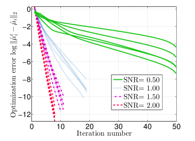
Figure 4: Plot of convergence behavior for different SNR, where for each curve, different parameters were chosen. The parameter settings are $d=10$, $n=1000$ and $\rho_{\mathrm{mix}}=0.6$.

5 Proofs

In this section, we collect the proofs of our main results. In all cases, we provide the main bodies of the proofs here, deferring the more technical details to the appendices.

5.1 Proof of Theorem 1

Throughout this proof, we make use of the shorthand $\widetilde{\rho}_{\mathrm{mix}}=1-\epsilon_{\mathrm{mix}}\makebox[0.0pt][l]{\hskip 1.29167pt\rule[5.59721pt]{4.18816pt}{0.43057pt}}{\pi}_{\min}$. Also we denote the separate components of the population EM operators by $\makebox[0.0pt][l]{\hskip 2.05pt\rule[8.12498pt]{8.30453pt}{0.43057pt}}{M}(\theta)=:(\makebox[0.0pt][l]{\hskip 2.05pt\rule[8.12498pt]{8.30453pt}{0.43057pt}}{M}^{\mu}(\theta),\makebox[0.0pt][l]{\hskip 2.05pt\rule[8.12498pt]{8.30453pt}{0.43057pt}}{M}^{\beta}(\theta))^{T}$ and their truncated equivalents by $\makebox[0.0pt][l]{\hskip 2.05pt\rule[8.12498pt]{8.30453pt}{0.43057pt}}{M}^{k}(\theta)=:(\makebox[0.0pt][l]{\hskip 2.05pt\rule[8.12498pt]{8.30453pt}{0.43057pt}}{M}^{\mu,k}(\theta),\makebox[0.0pt][l]{\hskip 2.05pt\rule[8.12498pt]{8.30453pt}{0.43057pt}}{M}^{\beta,k}(\theta))^{T}$. We begin by proving the bound given in part (a). Since $\makebox[0.0pt][l]{\hskip 2.05pt\hskip 0.58333pt\rule[8.12498pt]{5.00858pt}{0.43057pt}}{Q}=\lim_{n\rightarrow\infty}{\mathbb{E}}[Q_{n}]$, we have

$$\|\makebox[0.0pt][l]{\hskip 2.05pt\hskip 0.58333pt\rule[8.12498pt]{5.00858pt}{0.43057pt}}{Q}-\makebox[0.0pt][l]{\hskip 2.05pt\hskip 0.58333pt\rule[8.12498pt]{5.00858pt}{0.43057pt}}{Q}^{k}\|_{\infty} =\|\lim_{n\rightarrow\infty}{\mathbb{E}}[Q_{n}]-\makebox[0.0pt][l]{\hskip 2.05pt\hskip 0.58333pt\rule[8.12498pt]{5.00858pt}{0.43057pt}}{Q}^{k}\|_{\infty}\;\leq\;\frac{Cs^{5}}{\epsilon_{\mathrm{mix}}^{8}\makebox[0.0pt][l]{\hskip 1.29167pt\rule[5.59721pt]{4.18816pt}{0.43057pt}}{\pi}_{\min}^{2}}\widetilde{\rho}_{\mathrm{mix}}^{k},$$

where we have exchanged the supremum and the limit before applying the bound (18). The same holds for the separate functions $\makebox[0.0pt][l]{\hskip 2.05pt\hskip 0.58333pt\rule[8.12498pt]{5.00858pt}{0.43057pt}}{Q}_{1},\makebox[0.0pt][l]{\hskip 2.05pt\hskip 0.58333pt\rule[8.12498pt]{5.00858pt}{0.43057pt}}{Q}_{2}$.

Using this bound and the fact that for $\makebox[0.0pt][l]{\hskip 2.05pt\hskip 0.58333pt\rule[8.12498pt]{5.00858pt}{0.43057pt}}{Q}_{1}$ we have $\makebox[0.0pt][l]{\hskip 2.05pt\hskip 0.58333pt\rule[8.12498pt]{5.00858pt}{0.43057pt}}{Q}_{1}(\makebox[0.0pt][l]{\hskip 2.05pt\rule[8.12498pt]{8.30453pt}{0.43057pt}}{M}^{\mu}(\theta)\mid\theta)\geq\makebox[0.0pt][l]{\hskip 2.05pt\hskip 0.58333pt\rule[8.12498pt]{5.00858pt}{0.43057pt}}{Q}_{1}(\makebox[0.0pt][l]{\hskip 2.05pt\rule[8.12498pt]{8.30453pt}{0.43057pt}}{M}^{\mu,k}(\theta)\mid\theta)$, we find that

$$\makebox[0.0pt][l]{\hskip 2.05pt\hskip 0.58333pt\rule[8.12498pt]{5.00858pt}{0.43057pt}}{Q}_{1}(\makebox[0.0pt][l]{\hskip 2.05pt\rule[8.12498pt]{8.30453pt}{0.43057pt}}{M}^{\mu}(\theta)\mid\theta)\geq\makebox[0.0pt][l]{\hskip 2.05pt\hskip 0.58333pt\rule[8.12498pt]{5.00858pt}{0.43057pt}}{Q}_{1}^{k}(\makebox[0.0pt][l]{\hskip 2.05pt\rule[8.12498pt]{8.30453pt}{0.43057pt}}{M}^{\mu,k}(\theta)\mid\theta)-\frac{Cs^{5}}{\epsilon_{\mathrm{mix}}^{8}\makebox[0.0pt][l]{\hskip 1.29167pt\rule[5.59721pt]{4.18816pt}{0.43057pt}}{\pi}_{\min}^{2}}\widetilde{\rho}_{\mathrm{mix}}^{k}.$$

Since $\makebox[0.0pt][l]{\hskip 2.05pt\rule[8.12498pt]{8.30453pt}{0.43057pt}}{M}^{\mu,k}(\theta)$ is optimal, the first-order conditions for optimality imply that

$$\langle\makebox[0.0pt][l]{\hskip 2.05pt\hskip 0.58333pt\rule[8.12498pt]{5.00858pt}{0.43057pt}}{Q}_{1}^{k}(\makebox[0.0pt][l]{\hskip 2.05pt\rule[8.12498pt]{8.30453pt}{0.43057pt}}{M}^{\mu,k}(\theta)\mid\theta),\,\theta-\makebox[0.0pt][l]{\hskip 2.05pt\rule[8.12498pt]{8.30453pt}{0.43057pt}}{M}^{\mu,k}(\theta)\rangle \leq 0\qquad\mbox{for all $\theta\in\mathbb{B}_{2}\big{(}r;\theta^{*}\big{)}$.}$$

By the strict concavity of $\makebox[0.0pt][l]{\hskip 2.05pt\hskip 0.58333pt\rule[8.12498pt]{5.00858pt}{0.43057pt}}{Q}^{k}(\cdot|\theta)$ for all $\theta$, we obtain

$$\frac{Cs^{5}}{\epsilon_{\mathrm{mix}}^{8}\makebox[0.0pt][l]{\hskip 1.29167pt\rule[5.59721pt]{4.18816pt}{0.43057pt}}{\pi}_{\min}^{2}}\widetilde{\rho}_{\mathrm{mix}}^{k} \geq\makebox[0.0pt][l]{\hskip 2.05pt\hskip 0.58333pt\rule[8.12498pt]{5.00858pt}{0.43057pt}}{Q}_{1}(\makebox[0.0pt][l]{\hskip 2.05pt\rule[8.12498pt]{8.30453pt}{0.43057pt}}{M}^{\mu}(\theta)\mid\theta)-\makebox[0.0pt][l]{\hskip 2.05pt\hskip 0.58333pt\rule[8.12498pt]{5.00858pt}{0.43057pt}}{Q}_{1}^{k}(\makebox[0.0pt][l]{\hskip 2.05pt\rule[8.12498pt]{8.30453pt}{0.43057pt}}{M}^{\mu}(\theta)\mid\theta)$$

$$\geq\makebox[0.0pt][l]{\hskip 2.05pt\hskip 0.58333pt\rule[8.12498pt]{5.00858pt}{0.43057pt}}{Q}_{1}^{k}(\makebox[0.0pt][l]{\hskip 2.05pt\rule[8.12498pt]{8.30453pt}{0.43057pt}}{M}^{\mu,k}(\theta)\mid\theta)-\makebox[0.0pt][l]{\hskip 2.05pt\hskip 0.58333pt\rule[8.12498pt]{5.00858pt}{0.43057pt}}{Q}_{1}^{k}(\makebox[0.0pt][l]{\hskip 2.05pt\rule[8.12498pt]{8.30453pt}{0.43057pt}}{M}^{\mu}(\theta)\mid\theta)-\frac{Cs^{5}}{\epsilon_{\mathrm{mix}}^{8}\makebox[0.0pt][l]{\hskip 1.29167pt\rule[5.59721pt]{4.18816pt}{0.43057pt}}{\pi}_{\min}^{2}}\widetilde{\rho}_{\mathrm{mix}}^{k}$$

$$\geq\frac{\lambda_{\mu}}{2}\|\makebox[0.0pt][l]{\hskip 2.05pt\rule[8.12498pt]{8.30453pt}{0.43057pt}}{M}^{\mu}(\theta)-\makebox[0.0pt][l]{\hskip 2.05pt\rule[8.12498pt]{8.30453pt}{0.43057pt}}{M}^{\mu,k}(\theta)\|^{2}_{2}-\frac{Cs^{5}}{\epsilon_{\mathrm{mix}}^{8}\makebox[0.0pt][l]{\hskip 1.29167pt\rule[5.59721pt]{4.18816pt}{0.43057pt}}{\pi}_{\min}^{2}}\widetilde{\rho}_{\mathrm{mix}}^{k}$$

and therefore $\|\makebox[0.0pt][l]{\hskip 2.05pt\rule[8.12498pt]{8.30453pt}{0.43057pt}}{M}^{\mu}(\theta)-\makebox[0.0pt][l]{\hskip 2.05pt\rule[8.12498pt]{8.30453pt}{0.43057pt}}{M}^{\mu,k}(\theta)\|^{2}_{2}\leq 4\frac{Cs^{5}}{\lambda\epsilon_{\mathrm{mix}}^{8}\makebox[0.0pt][l]{\hskip 0.90417pt\rule[3.91806pt]{2.9317pt}{0.3014pt}}{\pi}_{\min}^{2}}\widetilde{\rho}_{\mathrm{mix}}^{k}$. In particular, setting $\theta=\theta^{*}$ and identifiability, i.e. $\makebox[0.0pt][l]{\hskip 2.05pt\rule[8.12498pt]{8.30453pt}{0.43057pt}}{M}^{\mu}(\theta^{*})=\theta^{*}$, yields

$$\|\makebox[0.0pt][l]{\hskip 2.05pt\rule[8.12498pt]{8.30453pt}{0.43057pt}}{M}^{\mu,k}(\theta^{*})-\theta^{*}\|_{2}^{2}\leq 4\frac{Cs^{5}}{\lambda_{\mu}\epsilon_{\mathrm{mix}}^{6}\makebox[0.0pt][l]{\hskip 1.29167pt\rule[5.59721pt]{4.18816pt}{0.43057pt}}{\pi}_{\min}^{2}}\widetilde{\rho}_{\mathrm{mix}}^{k},$$

and the equivalent bound can be obtained for $\makebox[0.0pt][l]{\hskip 2.05pt\rule[8.12498pt]{8.30453pt}{0.43057pt}}{M}^{\beta,k}(\cdot)$ which yields the claim.

We now turn to the proof of part (b). Let us suppose that the recursive bound (27) holds, and use it to complete the proof of this claim. We first show that if $\widetilde{\mu}^{t}\in\mathbb{B}_{2}(r;\mu^{*})$, then we must have $\widetilde{\mu}^{t+1}\in\mathbb{B}_{2}(r;\mu^{*})$ as well. Indeed, if $\widetilde{\mu}^{t}\in\mathbb{B}_{2}(r;\mu^{*})$, then we have by triangle inequality and the $(L_{\mu},L_{\beta})$-FOS condition

$$\|\makebox[0.0pt][l]{\hskip 2.05pt\rule[8.12498pt]{8.30453pt}{0.43057pt}}{M}^{\mu,k}(\widetilde{\theta}^{t})-\mu^{*}\|_{2} \leq\|\makebox[0.0pt][l]{\hskip 2.05pt\rule[8.12498pt]{8.30453pt}{0.43057pt}}{M}^{\mu,k}(\widetilde{\theta}^{t})-\makebox[0.0pt][l]{\hskip 2.05pt\rule[8.12498pt]{8.30453pt}{0.43057pt}}{M}^{\mu,k}(\mu^{*},\widetilde{\beta}^{t})\|_{2}+\|\makebox[0.0pt][l]{\hskip 2.05pt\rule[8.12498pt]{8.30453pt}{0.43057pt}}{M}^{\mu,k}(\mu^{*},\widetilde{\beta}^{t})-\makebox[0.0pt][l]{\hskip 2.05pt\rule[8.12498pt]{8.30453pt}{0.43057pt}}{M}^{\mu,k}(\mu^{*},\beta^{*})\|_{2}+\|\makebox[0.0pt][l]{\hskip 2.05pt\rule[8.12498pt]{8.30453pt}{0.43057pt}}{M}^{\mu,k}(\theta^{*})-\mu^{*}\|_{2}$$

$$\leq\frac{L_{\mu,1}}{\lambda_{\mu}}\|\widetilde{\mu}^{t}-\mu^{*}\|_{2}+\frac{L_{\mu,2}}{\lambda_{\mu}}\|\widetilde{\beta}^{t}-\beta^{*}\|_{2}+\frac{\varphi(k)}{2}$$

$$\leq\kappa(r+\max_{\beta\in\Omega_{\beta}}\|\beta-\beta^{*}\|_{2})+\varphi(k)\leq r,$$

where the final step uses the assumed bound on $\varphi$. For the joint parameter update we in turn have

$$\|\makebox[0.0pt][l]{\hskip 2.05pt\rule[8.12498pt]{8.30453pt}{0.43057pt}}{M}^{k}(\widetilde{\theta}^{t})-\theta^{*}\|_{\star} \leq\|\makebox[0.0pt][l]{\hskip 2.05pt\rule[8.12498pt]{8.30453pt}{0.43057pt}}{M}^{k}(\widetilde{\theta}^{t})-\makebox[0.0pt][l]{\hskip 2.05pt\rule[8.12498pt]{8.30453pt}{0.43057pt}}{M}^{k}(\theta^{*})\|_{\star}+\|\makebox[0.0pt][l]{\hskip 2.05pt\rule[8.12498pt]{8.30453pt}{0.43057pt}}{M}^{k}(\theta^{*})-\theta^{*}\|_{\star}$$

$$\leq\kappa\|\widetilde{\theta}^{t}-\theta^{*}\|_{\star}+\varphi(k).$$ (35)

By repeatedly applying inequality (5.1) and summing the geometric series, the claimed bound (26) follows.

It remains to prove the bound (27). Since the vector $\makebox[0.0pt][l]{\hskip 2.05pt\rule[8.12498pt]{8.30453pt}{0.43057pt}}{M}^{k}(\theta^{*})$ maximizes the function $\theta\mapsto\makebox[0.0pt][l]{\hskip 2.05pt\hskip 0.58333pt\rule[8.12498pt]{5.00858pt}{0.43057pt}}{Q}_{1}^{k}(\theta\mid\theta^{*})$, we have the first-order optimality condition

$$\langle\nabla\makebox[0.0pt][l]{\hskip 2.05pt\hskip 0.58333pt\rule[8.12498pt]{5.00858pt}{0.43057pt}}{Q}_{1}^{k}(\makebox[0.0pt][l]{\hskip 2.05pt\rule[8.12498pt]{8.30453pt}{0.43057pt}}{M}^{\mu,k}(\theta^{*})\mid\theta^{*}),\,\makebox[0.0pt][l]{\hskip 2.05pt\rule[8.12498pt]{8.30453pt}{0.43057pt}}{M}^{\mu,k}(\theta)-\makebox[0.0pt][l]{\hskip 2.05pt\rule[8.12498pt]{8.30453pt}{0.43057pt}}{M}^{\mu,k}(\theta^{*})\rangle \leq 0,\qquad\mbox{valid for any $\theta$.}$$

Similarly, we have $\langle\nabla\makebox[0.0pt][l]{\hskip 2.05pt\hskip 0.58333pt\rule[8.12498pt]{5.00858pt}{0.43057pt}}{Q}_{1}^{k}(\makebox[0.0pt][l]{\hskip 2.05pt\rule[8.12498pt]{8.30453pt}{0.43057pt}}{M}^{\mu,k}(\theta)\mid\theta),\,\makebox[0.0pt][l]{\hskip 2.05pt\rule[8.12498pt]{8.30453pt}{0.43057pt}}{M}^{\mu,k}(\theta^{*})-\makebox[0.0pt][l]{\hskip 2.05pt\rule[8.12498pt]{8.30453pt}{0.43057pt}}{M}^{\mu,k}(\theta)\rangle\leq 0$, and adding together these two inequalities yields

$$0 \leq\langle\nabla\makebox[0.0pt][l]{\hskip 2.05pt\hskip 0.58333pt\rule[8.12498pt]{5.00858pt}{0.43057pt}}{Q}_{1}^{k}(\makebox[0.0pt][l]{\hskip 2.05pt\rule[8.12498pt]{8.30453pt}{0.43057pt}}{M}^{\mu,k}(\theta^{*})\mid\theta^{*})-\nabla\makebox[0.0pt][l]{\hskip 2.05pt\hskip 0.58333pt\rule[8.12498pt]{5.00858pt}{0.43057pt}}{Q}_{1}^{k}(\makebox[0.0pt][l]{\hskip 2.05pt\rule[8.12498pt]{8.30453pt}{0.43057pt}}{M}^{\mu,k}(\mu)\mid\theta),\,\makebox[0.0pt][l]{\hskip 2.05pt\rule[8.12498pt]{8.30453pt}{0.43057pt}}{M}^{\mu,k}(\theta^{*})-\makebox[0.0pt][l]{\hskip 2.05pt\rule[8.12498pt]{8.30453pt}{0.43057pt}}{M}^{\mu,k}(\theta)\rangle$$

On the other hand, by the $\lambda$-strong concavity condition, we have

$$\lambda_{\mu}\|\makebox[0.0pt][l]{\hskip 2.05pt\rule[8.12498pt]{8.30453pt}{0.43057pt}}{M}^{\mu,k}(\theta)-\makebox[0.0pt][l]{\hskip 2.05pt\rule[8.12498pt]{8.30453pt}{0.43057pt}}{M}^{\mu,k}(\theta^{*})\|_{2}^{2} \leq\langle\nabla\makebox[0.0pt][l]{\hskip 2.05pt\hskip 0.58333pt\rule[8.12498pt]{5.00858pt}{0.43057pt}}{Q}_{1}^{k}(\makebox[0.0pt][l]{\hskip 2.05pt\rule[8.12498pt]{8.30453pt}{0.43057pt}}{M}^{\mu,k}(\theta)\mid\theta^{*}))-\nabla\makebox[0.0pt][l]{\hskip 2.05pt\hskip 0.58333pt\rule[8.12498pt]{5.00858pt}{0.43057pt}}{Q}_{1}^{k}(\makebox[0.0pt][l]{\hskip 2.05pt\rule[8.12498pt]{8.30453pt}{0.43057pt}}{M}^{\mu,k}(\theta^{*})\mid\theta^{*}),\,\makebox[0.0pt][l]{\hskip 2.05pt\rule[8.12498pt]{8.30453pt}{0.43057pt}}{M}^{\mu,k}(\theta^{*})-\makebox[0.0pt][l]{\hskip 2.05pt\rule[8.12498pt]{8.30453pt}{0.43057pt}}{M}^{\mu,k}(\theta)\rangle$$

Combining these two inequalities yields

$$\lambda_{\mu}\|\makebox[0.0pt][l]{\hskip 2.05pt\rule[8.12498pt]{8.30453pt}{0.43057pt}}{M}^{\mu,k}(\theta)-\makebox[0.0pt][l]{\hskip 2.05pt\rule[8.12498pt]{8.30453pt}{0.43057pt}}{M}^{\mu,k}(\theta^{*})\|_{2}^{2} \leq\langle\nabla\makebox[0.0pt][l]{\hskip 2.05pt\hskip 0.58333pt\rule[8.12498pt]{5.00858pt}{0.43057pt}}{Q}_{1}^{k}(\makebox[0.0pt][l]{\hskip 2.05pt\rule[8.12498pt]{8.30453pt}{0.43057pt}}{M}^{\mu,k}(\theta)\mid\theta^{*})-\nabla\makebox[0.0pt][l]{\hskip 2.05pt\hskip 0.58333pt\rule[8.12498pt]{5.00858pt}{0.43057pt}}{Q}_{1}^{k}(\makebox[0.0pt][l]{\hskip 2.05pt\rule[8.12498pt]{8.30453pt}{0.43057pt}}{M}^{\mu,k}(\theta)\mid\theta),\,\makebox[0.0pt][l]{\hskip 2.05pt\rule[8.12498pt]{8.30453pt}{0.43057pt}}{M}^{\mu,k}(\theta^{*})-\makebox[0.0pt][l]{\hskip 2.05pt\rule[8.12498pt]{8.30453pt}{0.43057pt}}{M}^{\mu,k}(\theta)\rangle$$

$$\leq\big{[}L_{\mu_{1}}\|\mu-\mu^{*}\|_{2}+L_{\mu_{2}}\|\beta-\beta^{*}\|_{2}\,\big{]}\|\makebox[0.0pt][l]{\hskip 2.05pt\rule[8.12498pt]{8.30453pt}{0.43057pt}}{M}^{\mu,k}(\theta)-\makebox[0.0pt][l]{\hskip 2.05pt\rule[8.12498pt]{8.30453pt}{0.43057pt}}{M}^{\mu,k}(\theta^{*})\|_{2},$$

and similarly we obtain $\lambda_{\beta}\|\makebox[0.0pt][l]{\hskip 2.05pt\rule[8.12498pt]{8.30453pt}{0.43057pt}}{M}^{\beta,k}(\theta)-\makebox[0.0pt][l]{\hskip 2.05pt\rule[8.12498pt]{8.30453pt}{0.43057pt}}{M}^{\beta,k}(\theta^{*})\|_{2}\leq\big{[}L_{\beta_{1}}\|\mu-\mu^{*}\|_{2}+L_{\beta_{2}}\|\beta-\beta^{*}\|_{2}\,\big{]}$. Adding both inequalities yields the claim (27).

5.2 Proof of Theorem 2

By the triangle inequality, for any step, with probability at least $1-2\delta$, we have

$$\|\widehat{\theta}^{t+1}-\theta^{*}\|_{\star} \leq\|M_{n}(\widehat{\theta}^{t})-M_{n}^{k}(\widehat{\theta}^{t})\|_{\star}+\|M_{n}^{k}(\widehat{\theta}^{t})-\makebox[0.0pt][l]{\hskip 2.05pt\rule[8.12498pt]{8.30453pt}{0.43057pt}}{M}^{k}(\widehat{\theta}^{t})\|_{\star}+\|\makebox[0.0pt][l]{\hskip 2.05pt\rule[8.12498pt]{8.30453pt}{0.43057pt}}{M}^{k}(\widehat{\theta}^{t})-\theta^{*}\|_{\star}$$

$$\leq\varphi_{n}(\delta,k)+\epsilon_{n}(\delta,k)+\kappa\|\widehat{\theta}^{t}-\theta^{*}\|_{\star}+\varphi(k).$$

In order to see that the iterates do not leave $\mathbb{B}_{2}\big{(}r;\mu^{*}\big{)}$, observe that

$$\|\widehat{\mu}^{t+1}-\mu^{*}\|_{2} \leq\|M^{\mu}_{n}(\widehat{\theta}^{t})-M_{n}^{\mu,k}(\widehat{\theta}^{t})\|_{2}+\|M_{n}^{\mu,k}(\widehat{\theta}^{t})-\makebox[0.0pt][l]{\hskip 2.05pt\rule[8.12498pt]{8.30453pt}{0.43057pt}}{M}^{\mu,k}(\widehat{\theta}^{t})\|_{2}+\|\makebox[0.0pt][l]{\hskip 2.05pt\rule[8.12498pt]{8.30453pt}{0.43057pt}}{M}^{\mu,k}(\widehat{\theta}^{t})-\mu^{*}\|_{2}$$ (36)

$$\leq\varphi_{n}(\delta,k)+\epsilon^{\mu}_{n}(\delta,k)+\kappa(\|\widehat{\mu}^{t}-\mu^{*}\|_{2}+\max_{\beta\in\Omega_{\beta}}\|\beta-\beta^{*}\|_{2})+\frac{\varphi(k)}{2}.$$

Consequently, as long as $\|\widehat{\mu}^{t}-\mu^{*}\|_{2}\leq r$, we also have $\|\widehat{\mu}^{t+1}-\mu^{*}\|_{2}\leq r$ whenever

$$\varphi_{n}(\delta,k)+\varphi(k)+\epsilon^{\mu}_{n}(\delta,k) \leq(1-\kappa)\,r-\kappa\max_{\beta\in\Omega_{\beta}}\|\beta-\beta^{*}\|_{2}.$$

Combining inequality (36) with the equivalent bound for $\beta$, we obtain

$$\|\widehat{\theta}^{t}-\theta^{*}\|_{\star}\leq\kappa\|\widehat{\theta}^{t-1}-\theta^{*}\|_{\star}+2\varphi_{n}(\delta,k)+\epsilon_{n}(\delta,k)+\varphi(k)$$

Summing the geometric series yields the bound (29b).

5.3 Proof of Corollary 1

The boundedness condition (Assumption (17)) is easy to check since for $X\sim N(\mu^{*},\sigma^{2})$, the quantity $\sup\limits_{\mu\in\mathbb{B}_{2}(r;\mu^{*})}\mathbb{E}\big{[}\max\{\|X-\mu\|_{2},\|X+\mu\|_{2}\}\big{]}$ is finite for any choice of radius $r<\infty$.

By Theorem 1, the $k$-truncated population EM iterates satisfy the bound

$$\|\widetilde{\theta}^{t}-\theta^{*}\|_{\star} \leq\kappa^{t}\|\widetilde{\theta}^{0}-\theta^{*}\|_{\star}+\frac{1}{1-\kappa}\varphi(k),$$ (37)

if the strong concavity (21) and FOS conditions (22), (23) hold with suitable parameters.

In the remainder of proof—and the bulk of the technical work— we show that:

• strong concavity holds with $\lambda_{\mu}=1$ and $\lambda_{\beta}=1-b^{2}$;

• the FOS conditions hold with

  $$L_{\mu,1}=c\,\>(\eta^{2}+1)\varphi_{2}(\epsilon_{\mathrm{mix}})\eta^{2}\mathrm{e}^{-c\eta^{2}}, \quad\mbox{and}\quad L_{\mu,2}=c\sqrt{\|\mu^{*}\|_{2}^{2}+\sigma^{2}}\varphi_{2}(\epsilon_{\mathrm{mix}})\eta^{2}\mathrm{e}^{-c\eta^{2}}$$

  $$L_{\beta,1}=c\frac{1-b}{1+b}\varphi_{2}(\epsilon_{\mathrm{mix}})\eta^{2}\mathrm{e}^{-c\eta^{2}} \quad\mbox{and}\quad L_{\beta,2}=c\sqrt{\|\mu^{*}\|_{2}^{2}+\sigma^{2}}\varphi_{2}(\epsilon_{\mathrm{mix}})\eta^{2}\mathrm{e}^{-c\eta^{2}},$$

where $\varphi_{2}(\epsilon_{\mathrm{mix}}):\,=\left(\frac{1}{\log(1/(1-\epsilon_{\mathrm{mix}}))}+\frac{1}{\epsilon_{\mathrm{mix}}}\right)$. Substuting these choices into the bound (37) and performing some algebra yields the claim.

5.3.1 Establishing strong concavity

We first show concavity of $\makebox[0.0pt][l]{\hskip 2.05pt\hskip 0.58333pt\rule[8.12498pt]{5.00858pt}{0.43057pt}}{Q}_{1}^{k}(\cdot\mid\theta^{\prime})$ and $\makebox[0.0pt][l]{\hskip 2.05pt\hskip 0.58333pt\rule[8.12498pt]{5.00858pt}{0.43057pt}}{Q}_{2}^{k}(\cdot\mid\theta^{\prime})$ separately. For strong concavity of $\makebox[0.0pt][l]{\hskip 2.05pt\hskip 0.58333pt\rule[8.12498pt]{5.00858pt}{0.43057pt}}{Q}_{1}^{k}(\cdot\mid\theta^{\prime})$, observe that

$$\makebox[0.0pt][l]{\hskip 2.05pt\hskip 0.58333pt\rule[8.12498pt]{5.00858pt}{0.43057pt}}{Q}_{1}^{k}(\mu\mid\theta^{\prime})=-\frac{1}{2}\mathbb{E}\left[p(z_{0}=1\mid X_{-k}^{k};\theta^{\prime})\|X_{0}-\mu\|_{2}^{2}+(1-p(z_{0}=1|X_{-k}^{k};\theta^{\prime}))\|X_{0}+\mu\|_{2}^{2}+c]\right],$$

where $c$ is a quantity independent of $\mu$. By inspection, this function is strongly concave in $\mu$ with parameter $\lambda_{\mu}=1$.

On the other hand, we have

$$\makebox[0.0pt][l]{\hskip 2.05pt\hskip 0.58333pt\rule[8.12498pt]{5.00858pt}{0.43057pt}}{Q}_{2}^{k}(\beta\mid\theta^{\prime})=\mathbb{E}_{X_{-k}^{k}\mid\theta^{*}}\sum_{z_{0},z_{1}}p(z_{0},z_{1}\mid X_{-k}^{k};\theta^{\prime})\log\left(\frac{\mathrm{e}^{\beta z_{0}z_{1}}}{\mathrm{e}^{\beta}+\mathrm{e}^{-\beta}}\right).$$

This function has second derivative $\frac{\partial^{2}}{\partial\beta^{2}}\makebox[0.0pt][l]{\hskip 2.05pt\hskip 0.58333pt\rule[8.12498pt]{5.00858pt}{0.43057pt}}{Q}_{2}^{k}(\beta\mid\theta^{\prime})=-4\frac{\mathrm{e}^{-2\beta}}{(\mathrm{e}^{-2\beta}+1)^{2}}$. As a function of $\beta\in\Omega_{\beta}$, this second derivative is maximized at $\beta=\frac{1}{2}\log\big{(}\frac{1+b}{1-b}\big{)}$. Consequently, the function $\makebox[0.0pt][l]{\hskip 2.05pt\hskip 0.58333pt\rule[8.12498pt]{5.00858pt}{0.43057pt}}{Q}_{2}^{k}(\cdot\mid\theta^{\prime})$ is strongly concave with parameter $\lambda_{\beta}=1-b^{2}$.

5.3.2 Separate FOS conditions

We now turn to proving that the FOS conditions in equations (22) and (23) hold. A key ingredient in our proof is the fact that the conditional density $p(z_{-k}^{k}\mid x_{-k}^{k};\mu,\beta)$ belongs to the exponential family with parameters $\beta\in$, and $\gamma_{i}:\,=\frac{\langle\mu,\,x_{i}\rangle}{\sigma^{2}}\in$ for $i=-k,\ldots,k$. (See the book [29] for more details on exponential families.) In particular, we have

$$\underbrace{p(z_{-k}^{k}\mid x_{-k}^{k},\mu,\beta)}_{:\,=p(z_{-k}^{k};\gamma,\beta)} =\exp\left\{\sum_{\ell=-k}^{k}\gamma_{\ell}z_{\ell}+\beta\sum_{\ell=-k}^{k-1}z_{\ell}z_{\ell+1}-\Phi(\gamma,\beta)\right\},$$ (38)

where the function $h$ absorbs various coupling terms. Note that this exponential family is a specific case of the following exponential family distribution

$$\underbrace{\tilde{p}(z_{-k}^{k}\mid x_{-k}^{k},\mu,\beta)}_{:\,=\tilde{p}(z_{-k}^{k};\gamma,\beta)} =\exp\left\{\sum_{\ell=-k}^{k}\gamma_{\ell}z_{\ell}+\sum_{\ell=-k}^{k-1}\beta_{\ell}z_{\ell}z_{\ell+1}-\Phi(\gamma,\beta)\right\}.$$ (39)

The distribution in (38) corresponds to (39) with $\beta_{\ell}=\beta$ for all $\ell$ and the so-called partition function $\Phi$ is given by

$$\Phi(\gamma,\beta)=\log\sum_{z}\exp\left\{\sum_{\ell=-k}^{k}\gamma_{\ell}z_{\ell}+\sum_{\ell=-k}^{k-1}\beta_{\ell}z_{\ell}z_{\ell+1}\right\}.$$

The reason to view our distribution as a special case of the more general one in (39) becomes clear when we consider the equivalence of expectations and the derivatives of the cumulant function

$$\left.\frac{\partial\Phi}{\partial\gamma_{\ell}}\right|_{\theta^{\prime}} =\mathbb{E}_{Z_{-k}^{k}|x_{-k}^{k},\theta^{\prime}}Z_{\ell}\>\>\text{ and }\>\>\left.\frac{\partial\Phi}{\partial\beta_{0}}\right|_{\theta^{\prime}}=\mathbb{E}_{Z_{-k}^{k}|x_{-k}^{k},\theta^{\prime}}Z_{0}Z_{1},$$ (40)

where we recall that $\mathbb{E}_{Z_{-k}^{k}|x_{-k}^{k},\theta^{\prime}}$ is the expectation with respect to the distribution $\tilde{p}(Z_{-k}^{k}\mid x_{-k}^{k};\mu^{\prime},\beta^{\prime})$ with $\beta_{\ell}=\beta^{\prime}$. Note that in the following any value $\theta^{\prime}$ for $\tilde{p}$ is taken to be on the manifold on which $\beta_{\ell}=\beta^{\prime}$ for some $\beta^{\prime}$ since this is the manifold the algorithm works on. Also, as before, $\mathbb{E}$ denotes the expectation over the joint distribution of all samples $X_{\ell}$ drawn according to $p(\cdot;\theta^{*})$, in this case $X_{-k}^{k}$.

Similarly to equations (40), the covariances of the sufficient statistics correspond to the second derivatives of the cumulant function

$$\left.\frac{\partial^{2}\Phi}{\partial\beta_{\ell}\partial\beta_{0}}\right|_{\theta} =\operatorname{cov}(Z_{0}Z_{1},Z_{\ell}Z_{\ell+1}\mid X_{-k}^{k},\theta)$$ (41a)

$$\left.\frac{\partial^{2}\Phi}{\partial\gamma_{\ell}\partial\gamma_{0}}\right|_{\theta} =\operatorname{cov}(Z_{0},Z_{\ell}\mid X_{-k}^{k},\theta)$$ (41b)

$$\left.\frac{\partial^{2}\Phi}{\partial\beta_{\ell}\partial\gamma_{0}}\right|_{\theta} =\operatorname{cov}(Z_{0},Z_{\ell}Z_{\ell+1}\mid X_{-k}^{k},\theta).$$ (41c)

In the following, we adopt the shorthand

$$\operatorname{cov}(Z_{\ell},Z_{\ell+1}\mid\gamma^{\prime},\beta^{\prime}) =\operatorname{cov}(Z_{\ell},Z_{\ell+1}\mid X_{-k}^{k},\theta^{\prime})$$

$$=\mathbb{E}_{Z_{\ell}^{\ell+1}|X_{-k}^{k},\theta^{\prime}}(Z_{\ell}-\mathbb{E}_{Z_{\ell}^{\ell+1}|X_{-k}^{k},\theta^{\prime}}Z_{\ell})(Z_{\ell+1}-\mathbb{E}_{Z_{\ell}^{\ell+1}|X_{-k}^{k},\theta^{\prime}}Z_{\ell+1})$$

where the dependence on $\beta$ is occasionally omitted so as to simplify notation.

5.3.3 Proof of inequality (22a)

By an application of the mean value theorem, we have

$$\|\nabla_{\mu}\makebox[0.0pt][l]{\hskip 2.05pt\hskip 0.58333pt\rule[8.12498pt]{5.00858pt}{0.43057pt}}{Q}_{1}^{k}(\mu\mid\mu^{\prime},\beta^{\prime})-\nabla_{\mu}\makebox[0.0pt][l]{\hskip 2.05pt\hskip 0.58333pt\rule[8.12498pt]{5.00858pt}{0.43057pt}}{Q}_{1}^{k}(\mu\mid\mu^{*},\beta^{\prime})\| \leq\underbrace{\left\|\mathbb{E}\sum_{\ell=-k}^{k}\left.\frac{\partial^{2}\Phi}{\partial\gamma_{\ell}\partial\gamma_{0}}\right|_{\theta=\widetilde{\theta}}(\gamma^{\prime}_{\ell}-\gamma^{*}_{\ell})X_{0}\right\|}_{T_{1}}$$

where $\widetilde{\theta}=\theta^{\prime}+t(\theta^{*}-\theta^{\prime})$ for some $t\in(0,1)$. Since second derivatives yield covariances (see equation (41)), we can write

$$T_{1} =\left\|\sum_{\ell=-k}^{k}\left.\mathbb{E}X_{0}\mathbb{E}\left[\operatorname{cov}(Z_{0},Z_{\ell}\mid\widetilde{\gamma})\frac{\langle\mu^{\prime}-\mu^{*},X_{\ell}\rangle}{\sigma^{2}}\right|X_{0}\right]\right\|_{2},$$

so that it suffices to control the expected conditional covariance. By the Cauchy-Schwarz inequality and the fact that $\operatorname{cov}(XY)\leq\sqrt{\operatorname{var}X}\sqrt{\operatorname{var}Y}$ and $\operatorname{var}(Z_{0}\mid X)\leq 1$, we obtain the following bound on the expected conditional covariance by using Lemma 4 (see Appendix B.1)

$$\mathbb{E}\left[\big{|}\operatorname{cov}(Z_{0},Z_{\ell}\mid\widetilde{\gamma})\mid X_{0}\big{|}\right] \leq\sqrt{\mathbb{E}\left[\operatorname{var}(Z_{0}\mid\widetilde{\gamma})\mid X_{0}\right]}\sqrt{\mathbb{E}\left[\operatorname{var}(Z_{\ell}\mid\widetilde{\gamma})\mid X_{0}\right]}$$

$$\leq\sqrt{\operatorname{var}(Z_{0}\mid\widetilde{\gamma}_{0})}.$$ (42a)

Furthermore, by Lemma 5 and 6 (see Appendix B.1), we have

$$|\operatorname{cov}(Z_{0},Z_{\ell}\mid\widetilde{\gamma})| \leq 2\rho_{\mathrm{mix}}^{\ell},\quad\mbox{and}\quad\left\|\mathbb{E}(\operatorname{var}(Z_{0}|\widetilde{\gamma}_{0}))^{1/2}X_{0}X_{0}^{T}\right\|_{op}\leq C\mathrm{e}^{-c\eta^{2}}.$$ (42b)

From the definition of the operator norm, we have

$$\|\mathbb{E}\operatorname{cov}(Z_{0},Z_{\ell}\mid\widetilde{\gamma})X_{0}X_{\ell}^{T}\big{\|}_{op} =\sup_{\begin{subarray}{c}\|u\|_{2}=1\\ \|v\|_{2}=1\end{subarray}}\mathbb{E}\operatorname{cov}(Z_{0},Z_{\ell}\mid\widetilde{\gamma})\langle X_{0},\,v\rangle\,\langle X_{\ell},\,u\rangle$$

$$\leq\sup_{\|v\|_{2}=1}\mathbb{E}|\operatorname{cov}(Z_{0},Z_{\ell}\mid\widetilde{\gamma})|\langle X_{0},\,v\rangle^{2}+\sup_{\|u\|_{2}=1}\mathbb{E}|\operatorname{cov}(Z_{0},Z_{\ell}\mid\widetilde{\gamma})|\langle X_{\ell},\,u\rangle^{2}$$

$$=\|\mathbb{E}X_{0}X_{0}^{T}\mathbb{E}\big{[}|\operatorname{cov}(Z_{0},Z_{\ell}\mid\widetilde{\gamma})\mid X_{0}\big{]}\|_{op}+\|\mathbb{E}X_{\ell}X_{\ell}^{T}\mathbb{E}\big{[}\operatorname{cov}(Z_{0},Z_{\ell}\mid\widetilde{\gamma})\mid X_{\ell}\big{]}\|_{op}$$

$$\stackrel{{\scriptstyle(i)}}{{\leq}}2\min\{\rho_{\mathrm{mix}}^{|\ell|}\|\mathbb{E}X_{0}X_{0}^{T}\|_{op},\|\mathbb{E}\operatorname{var}(Z_{0}\mid\widetilde{\gamma}_{0})^{1/2}X_{0}X_{0}^{T}\|_{op}\}$$

$$\stackrel{{\scriptstyle(ii)}}{{\leq}}2\min\{(\|\mu^{*}\|_{2}^{2}+\sigma^{2})\rho_{\mathrm{mix}}^{|\ell|},C^{\prime}\mathrm{e}^{-c\eta^{2}}\},$$ (43)

where inequality (i) makes use of inequalities (42a) and (42b), and step (ii) makes use of the second inequality in line (42b).

Combining inequalities (42a) and (43), we find that

$$T_{1} \leq\frac{\|\mu^{\prime}-\mu^{*}\|_{2}}{\sigma^{2}}\sum_{\ell=-k}^{k}\|\mathbb{E}\operatorname{cov}(Z_{0},Z_{\ell}\mid\widetilde{\gamma})X_{0}X_{\ell}^{T}\big{\|}_{op}$$

$$\leq 2\frac{\|\mu^{\prime}-\mu^{*}\|_{2}}{\sigma^{2}}\sum_{\ell=-k}^{k}\min\{(\|\mu^{*}\|_{2}^{2}+\sigma^{2})\rho_{\mathrm{mix}}^{|\ell|},C\mathrm{e}^{-c\eta^{2}}\}$$

$$\leq 4(\eta^{2}+1)\big{(}mC\mathrm{e}^{-c\eta^{2}}+\frac{\rho_{\mathrm{mix}}^{m}}{1-\rho_{\mathrm{mix}}}\big{)}\|\mu^{\prime}-\mu^{*}\|_{2}.$$

The last inequality follows from the proof of Corollary 1 in the paper [14] if $\eta^{2}>C$ for some universal constant $C$. By choosing $m=\frac{c\eta^{2}}{\log(1/\rho_{\mathrm{mix}})}$ so as to optimize the tradeoff, we have shown that

$$\|\nabla_{\mu}\makebox[0.0pt][l]{\hskip 2.05pt\hskip 0.58333pt\rule[8.12498pt]{5.00858pt}{0.43057pt}}{Q}_{1}^{k}(\mu\mid\mu^{\prime},\beta^{\prime})-\nabla_{\mu}\makebox[0.0pt][l]{\hskip 2.05pt\hskip 0.58333pt\rule[8.12498pt]{5.00858pt}{0.43057pt}}{Q}_{1}^{k}(\mu\mid\mu^{*},\beta^{\prime})\| \leq L_{\mu,1}\|\mu^{\prime}-\mu^{*}\|_{2},$$

where $L_{\mu,1}=c\,\>\varphi_{1}(\eta)\varphi_{2}(\epsilon_{\mathrm{mix}})\eta^{2}\mathrm{e}^{-c\eta^{2}}$ as claimed.

5.3.4 Proof of inequality (22b)

The same argument via the mean value theorem guarantees that

$$\|\frac{\partial}{\partial\beta}\makebox[0.0pt][l]{\hskip 2.05pt\hskip 0.58333pt\rule[8.12498pt]{5.00858pt}{0.43057pt}}{Q}_{2}^{k}(\beta\mid\mu^{\prime},\beta^{\prime})-\frac{\partial}{\partial\beta}\makebox[0.0pt][l]{\hskip 2.05pt\hskip 0.58333pt\rule[8.12498pt]{5.00858pt}{0.43057pt}}{Q}_{2}^{k}(\beta\mid\mu^{\prime},\beta^{*})\| \leq\left\|\mathbb{E}\sum_{\ell=-k}^{k}\left.\frac{\partial^{2}\Phi}{\partial\beta_{\ell}\partial\gamma_{0}}\right|_{\theta=\widetilde{\theta}}(\beta^{\prime}-\beta^{*})X_{0}\right\|_{2}.$$

In order to bound this quantity, we again use the equivalence (41) and bound the expected conditional covariance. Furthermore, Lemma 5 and 6 yield

$$\operatorname{cov}(Z_{0},Z_{\ell}Z_{\ell+1}\mid\widetilde{\gamma})\stackrel{{\scriptstyle(i)}}{{\leq}}2\rho_{\mathrm{mix}}^{\ell}\quad\mbox{and}\quad\left\|\mathbb{E}\operatorname{var}(Z_{0}\mid\widetilde{\gamma}_{0})X_{0}X_{0}^{T}\right\|_{op}\stackrel{{\scriptstyle(ii)}}{{\leq}}c\mathrm{e}^{-c\eta^{2}}.$$ (44)

Here inequality (ii) follows by combining inequality (54c) from Lemma 5 with the fact that $\operatorname{var}(Z_{0}\mid\widetilde{\gamma}_{0})\leq 1$.

$$\|\mathbb{E}X_{0}\operatorname{cov}(Z_{0},Z_{\ell}Z_{\ell+1}\mid\widetilde{\gamma})\|_{2} =\sup_{\|u\|_{2}=1}\mathbb{E}\langle X_{0},u\rangle\operatorname{cov}(Z_{0},Z_{\ell}Z_{\ell+1}\mid\widetilde{\gamma})$$

$$\leq\sup_{\|u\|_{2}=1}\mathbb{E}|\langle X_{0},u\rangle|\mathbb{E}\big{[}|\operatorname{cov}(Z_{0},Z_{\ell}Z_{\ell+1}\mid\widetilde{\gamma})|\mid X_{0}\big{]}$$

$$\stackrel{{\scriptstyle(iii)}}{{\leq}}\sup_{\|u\|_{2}=1}\mathbb{E}|\langle X_{0},u\rangle|\min\{\rho_{\mathrm{mix}}^{|\ell|},(\operatorname{var}(Z_{0}\mid\widetilde{\gamma}_{0}))^{1/2}\}$$

$$\stackrel{{\scriptstyle(iv)}}{{\leq}}\min\{\sup_{\|u\|_{2}=1}\sqrt{\mathbb{E}\langle X_{0},u\rangle^{2}}\rho_{\mathrm{mix}}^{|\ell|},\sup_{\|u\|_{2}=1}\sqrt{\mathbb{E}\langle X_{0},u\rangle^{2}\operatorname{var}(Z_{0}\mid\widetilde{\gamma}_{0}))}\}$$

$$\stackrel{{\scriptstyle(v)}}{{\leq}}\min\{\rho_{\mathrm{mix}}^{|\ell|}\sqrt{\|\mathbb{E}X_{0}X_{0}^{T}\|_{op}},\sqrt{\|\mathbb{E}\operatorname{var}(Z_{0}\mid\widetilde{\gamma}_{0})X_{0}X_{0}^{T}\|_{op}}\}$$

$$\stackrel{{\scriptstyle(vi)}}{{\leq}}\min\{\rho_{\mathrm{mix}}^{|\ell|}\sqrt{\|\mu^{*}\|_{2}^{2}+\sigma^{2}},C\mathrm{e}^{-c\eta^{2}}\}$$

where step (iii) uses inequality (44); step (iv) follows from the Cauchy-Schwarz inequality; step (v) follows from the definition of the operator norm; and step (vi) uses inequality (44) again.

Putting together the pieces, we find that

$$\left\|\mathbb{E}\sum_{\ell=-k}^{k}\frac{\partial^{2}\Phi}{\partial\beta_{\ell}\partial\gamma_{0}}X_{0}\right\|_{2}|\beta^{\prime}-\beta^{*}| \leq\sum_{\ell=-k}^{k}\left\|\mathbb{E}X_{0}\mathbb{E}[\operatorname{cov}(Z_{0},Z_{\ell}Z_{\ell+1}\mid\widetilde{\gamma})\mid X_{0}]\right\|_{2}|\beta^{\prime}-\beta^{*}|$$

$$\leq 4\sqrt{\|\mu^{*}\|_{2}^{2}+\sigma^{2}}\left(c\,m\,\mathrm{e}^{-c\eta^{2}}+\frac{\rho_{\mathrm{mix}}^{m}}{1-\rho_{\mathrm{mix}}}\right)|\beta^{\prime}-\beta^{*}|.$$

Setting $m=\frac{c\eta^{2}}{\log(1/\rho_{\mathrm{mix}})}$ to balance the tradeoff between the two terms, we find that inequality (22b) holds with $L_{\mu,2}=c\varphi_{2}(\epsilon_{\mathrm{mix}})\sqrt{\|\mu^{*}\|_{2}+\sigma^{2}}\eta^{2}\mathrm{e}^{-c\eta^{2}}$, as claimed.

5.3.5 Proof of inequality (23a)

By the same argument via the mean value theorem, we find that

$$\big{\|}\frac{\partial}{\partial\beta}\makebox[0.0pt][l]{\hskip 2.05pt\hskip 0.58333pt\rule[8.12498pt]{5.00858pt}{0.43057pt}}{Q}_{2}^{k}(\beta\mid\beta^{\prime},\mu^{\prime})-\frac{\partial}{\partial\beta}\makebox[0.0pt][l]{\hskip 2.05pt\hskip 0.58333pt\rule[8.12498pt]{5.00858pt}{0.43057pt}}{Q}_{2}^{k}(\beta\mid\beta^{\prime},\mu^{*})\big{\|} \leq\Big{|}\mathbb{E}\sum_{\ell=-k}^{k}\left.\frac{\partial^{2}\Phi}{\partial\gamma_{\ell}\partial\beta_{0}}\right|_{\theta=\widetilde{\theta}}\frac{\langle\mu^{\prime}-\mu^{*},X_{\ell}\rangle}{\sigma^{2}}\Big{|}.$$

Equation (41) guarantees that $\frac{\partial^{2}\Phi}{\partial\gamma_{\ell}\partial\beta_{0}}=\operatorname{cov}(Z_{0}Z_{1},Z_{\ell}\mid\gamma)$. Therefore, by similar arguments as in the proof of inequalities (22), we have

$$T :\,=\Big{|}\sum_{\ell=-k}^{k}\mathbb{E}\langle\mu^{\prime}-\mu^{*},X_{\ell}\rangle\mathbb{E}[\operatorname{cov}(Z_{0}Z_{1},Z_{\ell}\mid\widetilde{\gamma}_{\ell},\beta^{\prime})|X_{\ell}]\Big{|}$$

$$\leq\Big{|}\sum_{\ell=-k}^{k}\mathbb{E}|\langle\mu^{\prime}-\mu^{*},X_{\ell}\rangle|\min\{\rho_{\mathrm{mix}}^{|\ell|},(\operatorname{var}(Z_{\ell}\mid\widetilde{\gamma}_{\ell},\beta^{\prime}))^{1/2}\}\Big{|}$$

$$\leq\Big{|}\sum_{\ell=-k}^{k}\min\big{\{}\rho_{\mathrm{mix}}^{|\ell|},\sqrt{\mathbb{E}\operatorname{var}(Z_{\ell}\mid\widetilde{\gamma}_{\ell},\beta^{\prime})}\big{\}}\sqrt{\mathbb{E}\langle\mu^{\prime}-\mu^{*},X_{\ell}\rangle^{2}}\Big{|}$$

$$\leq\sqrt{\|\mu^{*}\|^{2}_{2}+\sigma^{2}}\big{(}mc\,\mathrm{e}^{-c\eta^{2}}+2\sum_{\ell=m+1}^{k}\rho_{\mathrm{mix}}^{\ell}\big{)}.$$

where we have used inequality (54b) from Lemma 6. Finally, setting $m=\frac{c\eta^{2}}{\log(1/\rho_{\mathrm{mix}})}$ yields that the FOS condition holds with $L_{\beta,2}=c\sqrt{\|\mu^{*}\|_{2}+\sigma^{2}}\varphi_{2}(\epsilon_{\mathrm{mix}})\eta^{2}\mathrm{e}^{-c\eta^{2}}$, as claimed.

5.3.6 Proof of inequality (23b)

By the same mean value argument, we find that

$$\|\frac{\partial}{\partial\beta}\makebox[0.0pt][l]{\hskip 2.05pt\hskip 0.58333pt\rule[8.12498pt]{5.00858pt}{0.43057pt}}{Q}_{2}^{k}(\beta\mid\beta^{\prime},\mu^{\prime})-\frac{\partial}{\partial\beta}\makebox[0.0pt][l]{\hskip 2.05pt\hskip 0.58333pt\rule[8.12498pt]{5.00858pt}{0.43057pt}}{Q}_{2}^{k}(\beta\mid\beta^{*},\mu^{\prime})\big{\|} \leq\Big{|}\mathbb{E}\sum_{\ell=-k}^{k}\left.\frac{\partial^{2}\Phi}{\partial\beta_{\ell}\partial\beta_{0}}\right|_{\theta=\widetilde{\theta}}(\beta^{\prime}-\beta^{*})\Big{|}.$$

By the exponential family view in equality (41) it suffices to control the expected conditional covariance. Lemma 5 and 6 guarantee that

$$|\operatorname{cov}(Z_{0}Z_{1},Z_{\ell}Z_{\ell+1}\mid X_{-k}^{k},\widetilde{\gamma})| \leq\rho_{\mathrm{mix}}^{|\ell|},\quad\mbox{and}\quad\mathbb{E}\operatorname{var}(Z_{0}Z_{1}\mid\widetilde{\gamma}_{0}^{1},\widetilde{\beta})\leq c\,\frac{1+b}{1-b}\;\mathrm{e}^{-c\eta^{2}}.$$ (45)

Furthermore, the Cauchy-Schwarz inequality combined with the bound (53a) from Lemma 4 yields

$$\mathbb{E}\big{|}\operatorname{cov}(Z_{0}Z_{1},Z_{\ell}Z_{\ell+1}\mid\widetilde{\gamma})\big{|} \leq\sqrt{\mathbb{E}\operatorname{var}(Z_{0}Z_{1}\mid\widetilde{\gamma}_{-k}^{k},\widetilde{\beta})}\sqrt{\mathbb{E}\operatorname{var}(Z_{\ell}Z_{\ell+1}\mid\widetilde{\gamma}_{-k}^{k},\widetilde{\beta})}$$

$$\leq\sqrt{\mathbb{E}\operatorname{var}(Z_{0}Z_{1}\mid\widetilde{\gamma}_{0}^{1},\widetilde{\beta})}\sqrt{\mathbb{E}\operatorname{var}(Z_{\ell}Z_{\ell+1}\mid\widetilde{\gamma}_{\ell}^{\ell+1},\widetilde{\beta})}$$

$$\leq\mathbb{E}\operatorname{var}(Z_{0}Z_{1}\mid\widetilde{\gamma}_{0}^{1},\widetilde{\beta}).$$ (46)

Combining the bounds (45) and (46) yields

$$\left|\sum_{\ell=-k}^{k}\mathbb{E}\frac{\partial^{2}\Phi}{\partial\beta_{\ell}\partial\beta_{0}}(\beta^{\prime}-\beta^{*})\right| \leq\sum_{\ell=-k}^{k}\big{|}\mathbb{E}\operatorname{cov}(Z_{0}Z_{1},Z_{\ell}Z_{\ell+1}\mid\widetilde{\gamma}_{-k}^{k},\widetilde{\beta})\big{|}\;|\beta^{\prime}-\beta^{*}|$$

$$\leq\sum_{\ell=-k}^{k}\min\left\{\rho_{\mathrm{mix}}^{|\ell|},\mathbb{E}\operatorname{var}(Z_{0}Z_{1}\mid\widetilde{\gamma}_{0}^{1},\widetilde{\beta})\right\}|\beta^{\prime}-\beta^{*}|$$

$$\leq 2\left(c\frac{1+b}{1-b}\,m\mathrm{e}^{-c\eta^{2}}+\sum_{l=m+1}^{k}\rho_{\mathrm{mix}}^{\ell}\right)|\beta^{\prime}-\beta^{*}|$$

$$\leq 2c\frac{1+b}{1-b}\varphi_{2}(\epsilon_{\mathrm{mix}})\eta^{2}\mathrm{e}^{-c\eta^{2}}|\beta^{\prime}-\beta^{*}|$$

where the final inequality follows by setting $m=\frac{c\eta^{2}}{\log(1/\rho_{\mathrm{mix}})}$. Therefore, the FOS condition holds with $L_{\beta,1}=c\frac{1-b}{1+b}\varphi_{2}(\epsilon_{\mathrm{mix}})\eta^{2}\mathrm{e}^{-c\eta^{2}}$, as claimed.

5.4 Proof of Corollary 2

In order to prove this corollary, it is again convenient to separate the updates on the mean vectors $\mu$ from those applied to the transition parameter $\beta$. Recall the definitions of $\varphi$, $\varphi_{n}$ and $\epsilon_{n}$ from equations (25) and (28a) respectively.

Using Theorem 2 we readily have that given any initialization $\widehat{\theta}^{0}\in\Omega$, with probability at least $1-2\delta$, we are guaranteed that

$$\|\widehat{\theta}^{T}-\theta^{*}\|_{\star}\leq\kappa^{T}\|\widehat{\theta}^{0}-\theta^{*}\|_{\star}+\frac{2\varphi_{n}(\delta,k)+\epsilon_{n}(\delta,k)+\varphi(k)}{1-\kappa}.$$ (47)

In order to leverage the bound (47), we need to find appropriate upper bounds on the quantities $\varphi_{n}(\delta,k)$, $\epsilon_{n}(\delta,k)$.

Lemma 1.

Suppose that the truncation level satisifes the lower bound

$$k \geq\log\left(\frac{C_{\epsilon}n}{\delta}\right)\;\Big{(}\log\frac{1}{(1-\frac{\epsilon_{\mathrm{mix}}}{2})}\Big{)}^{-1}\qquad\mbox{where $C_{\epsilon}:\,=\frac{36}{\epsilon_{\mathrm{mix}}^{3}}$.}$$ (48a)

Then with the radius $$r=\frac{\|\mu^{*}\|_{2}}{4}$$, we have

$$\epsilon^{\mu}_{n}\big{(}\delta,k\big{)} \leq C_{0}\|\mu^{*}\|_{2}\big{(}\frac{\|\mu^{*}\|_{2}^{2}}{\sigma^{2}}+1\big{)}\log(k^{2}/\delta)\sqrt{\frac{k^{3}d\log n}{n}},\quad\mbox{and}$$ (48b)

$$\epsilon^{\beta}_{n}\big{(}\delta,k\big{)} \leq C_{0}\;\frac{\sqrt{\|\mu^{*}\|_{2}^{2}+\sigma^{2}}}{\sigma^{2}}\sqrt{\frac{k^{3}\log(k^{2}/\delta)}{n}}.$$ (48c)

Lemma 2.

Suppose that the SNR $\eta^{2}=\frac{\|\mu^{*}\|_{2}^{2}}{\sigma^{2}}$ is lower bounded as $\eta^{2}\geq C(\log\log d+\log\|\mu^{*}\|_{2})$ for a sufficiently large $C$. Then with the radius $r=\frac{\|\mu^{*}\|_{2}}{4}$, we have

$$\varphi^{2}_{n}(\delta,k) \leq C_{1}\;\Big{\{}\frac{1}{\sigma}\sqrt{\frac{d\log^{2}(C_{\epsilon}n/\delta)}{n}}+\frac{\|\mu^{*}\|_{2}}{\sigma}\sqrt{\frac{\log^{2}(C_{\epsilon}n/\delta)}{n}}+\frac{\|\mu^{*}\|_{2}^{2}}{\sigma^{2}}\Big{\}}\;\varphi^{2}(k).$$ (49)

See Appendices C.1 and C.2, respectively, for the proofs of these two lemmas.

Using these two lemmas, we can now complete the proof of the corollary. From the definition (32) of $\kappa$, under the stated lower bound on $\eta^{2}$, we can ensure that $\kappa\big{\{}\frac{4\log\frac{1+b}{1-b}}{\|\mu^{*}\|_{2}}\big{\}}\leq 1/2$. Under this condition, inequality (29a) with $r=\|\mu^{*}\|_{2}/4$ reduces to showing that

$$\varphi_{n}(\delta,k)+\epsilon^{\mu}_{n}(\delta,k)+\varphi(k)\leq(1-2\kappa)\frac{\|\mu^{*}\|_{2}}{8}.$$ (50)

As long as $n\geq C_{1}(\sigma^{2}+\|\mu^{*}\|_{2}^{2})d\log^{2}(d/\delta)$ for a sufficiently large $C_{1}$, we are guaranteed that the bound (50) holds. Now the specific choice (48a) of $k$ guarantees that

$$\varphi_{n}(\delta,k)+\epsilon^{\mu}_{n}(\delta,k)+\epsilon^{\beta}_{n}(\delta,k)+\varphi(k)\leq C\|\mu^{*}\|_{2}(\frac{\|\mu^{*}\|_{2}^{2}}{\sigma^{2}}+1)\log^{2}n\sqrt{\frac{d\log^{2}(n/\delta)}{n}}.$$ (51)

Substituting the bound (51) into inequality (47) completes the proof of the corollary.

6 Discussion

In this paper, we provided general global convergence guarantees for the Baum-Welch algorithm as well as specific results for a hidden Markov mixture of two isotropic Gaussians. In contrast to the classical perspective of focusing on the MLE, we focused on bounding the distance between the Baum-Welch iterates and the true parameter. Under suitable regularity conditions, our theory guarantees that the iterates converge to an $e_{n}$-ball of the true parameter, where $e_{n}$ represents a form of statistical error. It is important to note that our theory does not guarnatee convergence to the MLE itself, but rather to this ball that contains both the MLE and the true parameter. When applied to the Gaussian mixture HMM, we proved that the Baum-Welch algorithm achieves estimation error that is minimax optimal up to logarithmic factors. To the best of our knowledge, these are the first rigorous guarantees for the Baum-Welch algorithm that allow for a large initialization radius.

Acknowledgements

This work was partially supported by NSF grant CIF-31712-23800, ONR-MURI grant DOD-002888, and AFOSR grant FA9550-14-1-0016 to MJW.

Appendix A Proof of Proposition 1

In order to show that the limit $\lim_{n\to\infty}\mathbb{E}Q_{n}(\theta\mid\theta^{\prime})$ exists, it suffices to show that the sequence of functions $\{\mathbb{E}Q_{1},\mathbb{E}Q_{2},\ldots,\mathbb{E}Q_{n}\}$ is Cauchy in the sup-norm (as defined previously in equation (16)). In particular, it suffices to show that for every $\epsilon>0$ there is a positive integer $N(\epsilon)$ such that for $m,n\geq N(\epsilon)$,

$$\|\mathbb{E}Q_{m}-\mathbb{E}Q_{n}\|_{\infty}\leq\epsilon.$$

In order to do so, we make use of the previously stated bound (18) relating $\mathbb{E}Q_{n}$ to $\makebox[0.0pt][l]{\hskip 2.05pt\hskip 0.58333pt\rule[8.12498pt]{5.00858pt}{0.43057pt}}{Q}^{k}$. Taking this bound as given for the moment, an application of the triangle inequality yields

$$\|\mathbb{E}Q_{m}-\mathbb{E}Q_{n}\|_{\infty}\leq\|\mathbb{E}Q_{m}-\makebox[0.0pt][l]{\hskip 2.05pt\hskip 0.58333pt\rule[8.12498pt]{5.00858pt}{0.43057pt}}{Q}^{k}\|_{\infty}+\|\mathbb{E}Q_{n}-\makebox[0.0pt][l]{\hskip 2.05pt\hskip 0.58333pt\rule[8.12498pt]{5.00858pt}{0.43057pt}}{Q}^{k}\|_{\infty}\;\leq\;\epsilon,$$

the final inequality follows as long as we choose $N(\epsilon)$ and $k$ large enough (roughly proportional to $\log(1/\epsilon)$).

It remains to prove the claim (18). In order to do so, we require an auxiliary lemma:

Lemma 3 (Approximation by truncation).

For a Markov chain satisfying the mixing condition (3), we have

$$\sup_{\theta^{\prime}\in\Omega}\sup_{x}\sum_{z_{i}}|p(z_{i}\mid x_{1}^{n};\theta^{\prime})-p(z_{i}\mid x_{i-k}^{i+k};\theta^{\prime})|\leq\frac{Cs^{4}}{\epsilon_{\mathrm{mix}}^{8}\makebox[0.0pt][l]{\hskip 1.29167pt\rule[5.59721pt]{4.18816pt}{0.43057pt}}{\pi}_{\min}}\big{(}1-\epsilon_{\mathrm{mix}}\makebox[0.0pt][l]{\hskip 1.29167pt\rule[5.59721pt]{4.18816pt}{0.43057pt}}{\pi}_{\min}\big{)}^{k}$$ (52)

for all $i\in[0,n]$, where $\makebox[0.0pt][l]{\hskip 1.29167pt\rule[5.59721pt]{4.18816pt}{0.43057pt}}{\pi}_{\min}=\min_{j\in[s],\beta\in\Omega_{\beta}}\makebox[0.0pt][l]{\hskip 1.29167pt\rule[5.59721pt]{4.18816pt}{0.43057pt}}{\pi}(j;\beta)$.

See Appendix D.2 for the proof of this lemma.

Using Lemma 3, let us now prove the claim (18). Introducing the shorthand notation

$$h(X_{i},z_{i},\theta,\theta^{\prime}) :\,=\log p(X_{i}\mid z_{i};\theta)+\sum_{z_{i-1}}p(z_{i}\mid z_{i-1};\theta^{\prime})\log p(z_{i}|z_{i-1},\theta),$$

we can verify by applying Lemma 3 that

$$\|\mathbb{E}Q_{n}-\makebox[0.0pt][l]{\hskip 2.05pt\hskip 0.58333pt\rule[8.12498pt]{5.00858pt}{0.43057pt}}{Q}^{k}\|_{\infty} =\Big{|}\sup_{\theta,\theta^{\prime}}\frac{1}{n}\sum_{i=1}^{n}\sum_{z_{i}}\mathbb{E}(p(z_{i}\mid X_{1}^{n},\theta^{\prime})-p(z_{i}\mid X_{i-k}^{i+k},\theta^{\prime}))h(X_{i},z_{i},\theta,\theta^{\prime})\Big{|}$$

$$+\Big{|}\frac{1}{n}\sup_{\theta,\theta^{\prime}}\mathbb{E}\sum_{z_{0}}p(z_{0}\mid X_{1}^{n},\theta^{\prime})\log p(z_{0};\theta)\Big{|}$$

$$\leq\sup_{\theta,\theta^{\prime}}\sup_{x}\sum_{z_{i}}\big{|}p(z_{i}\mid x_{1}^{n},\theta^{\prime})-p(z_{i}\mid x_{i-k}^{i+k},\theta^{\prime})\big{|}\left[\mathbb{E}\frac{1}{n}\sum_{i=1}^{n}\max_{z_{i}\in[m]}|h(X_{i},z_{i},\theta,\theta^{\prime})|\right]+\frac{1}{n}\log\makebox[0.0pt][l]{\hskip 1.29167pt\rule[5.59721pt]{4.18816pt}{0.43057pt}}{\pi}_{\min}^{-1}$$

$$\leq\frac{cs^{4}}{\epsilon_{\mathrm{mix}}^{8}\makebox[0.0pt][l]{\hskip 1.29167pt\rule[5.59721pt]{4.18816pt}{0.43057pt}}{\pi}_{\min}}\big{(}1-\epsilon_{\mathrm{mix}}\makebox[0.0pt][l]{\hskip 1.29167pt\rule[5.59721pt]{4.18816pt}{0.43057pt}}{\pi}_{\min}\big{)}^{k}\left(\mathbb{E}\max_{z_{i}\in[m]}\big{|}\log p(X_{i}\mid z_{i},\theta)\big{|}+s\log\makebox[0.0pt][l]{\hskip 1.29167pt\rule[5.59721pt]{4.18816pt}{0.43057pt}}{\pi}_{\min}^{-1}\right)+\frac{1}{n}\log\makebox[0.0pt][l]{\hskip 1.29167pt\rule[5.59721pt]{4.18816pt}{0.43057pt}}{\pi}_{\min}^{-1}$$

$$\leq\frac{c^{\prime}\,s^{5}}{\epsilon_{\mathrm{mix}}^{8}\makebox[0.0pt][l]{\hskip 1.29167pt\rule[5.59721pt]{4.18816pt}{0.43057pt}}{\pi}_{\min}^{2}}\big{(}1-\epsilon_{\mathrm{mix}}\makebox[0.0pt][l]{\hskip 1.29167pt\rule[5.59721pt]{4.18816pt}{0.43057pt}}{\pi}_{\min}\big{)}^{k}+\frac{1}{n}\log\makebox[0.0pt][l]{\hskip 1.29167pt\rule[5.59721pt]{4.18816pt}{0.43057pt}}{\pi}_{\min}^{-1},$$

where the last inequality follows from the boundedness condition (17) on the log output densities.

Appendix B Technical details for Corollary 1

The proof of the corollary mainly involves proving the bound (37), and then showing that the conditions in the theorem hold for the special Gaussian output HMM.

B.1 Bounds on conditional variances

In this section, we collect some auxiliary bounds on conditional covariances in hidden Markov models. These results are used in the proof of Corollary 1.

Lemma 4.

For any HMM with observed-hidden states $(X_{i},Z_{i})$, we have

$$\mathbb{E}\left[\operatorname{var}(Z_{0}Z_{1}\mid X_{-k}^{k})\right] \leq\mathbb{E}\operatorname{var}(Z_{0}Z_{1}\mid X_{0}^{1})$$ (53a)

$$\mathbb{E}\left[\operatorname{var}(Z_{0}\mid X_{-k}^{k})\mid X_{0}\right] \leq\operatorname{var}(Z_{0}\mid X_{0})$$ (53b)

where we have omitted the dependence on the parameters.

Proof.

We use the law of total variance, which guarantees that $\operatorname{var}Z=\mathbb{E}\big{[}\operatorname{var}(Z\mid X)\big{]}+\operatorname{var}\mathbb{E}[Z\mid X]$. Using this decomposition, we have

$$\mathbb{E}[\operatorname{var}(Z_{0}\mid X_{0}^{1})\mid X_{0}] \leq\operatorname{var}(Z_{0}\mid X_{0})$$

$$\mathbb{E}[\operatorname{var}(Z_{0}Z_{1}\mid X_{0}^{2})\mid X_{0}^{1}] \leq\operatorname{var}(Z_{0}Z_{1}\mid X_{0}^{1}).$$

The result then follows by induction. ∎

We now show that the expected conditional variance of the hidden state (or pairs thereof) conditioned on the corresponding observation (pairs of observations) decays exponentially with the SNR.

Lemma 5.

For a $2$-state Markov chain with true parameter $\theta^{*}$, we have for $\mu\in\mathbb{B}_{2}\big{(}\frac{\|\mu^{*}\|_{2}}{4};\mu^{*}\big{)}$ and $\beta\in\Omega_{\beta}$

$$\left\|\mathbb{E}X_{0}X_{0}^{T}(\operatorname{var}(Z_{0}\mid\gamma_{0},\beta))^{1/2}\right\|_{op} \leq c_{0}\,\mathrm{e}^{-c\eta^{2}}$$ (54a)

$$\mathbb{E}\operatorname{var}(Z_{\ell}\mid\gamma_{\ell},\beta) \leq c_{0}\;\mathrm{e}^{-c\eta^{2}}$$ (54b)

$$\mathbb{E}\operatorname{var}(Z_{0}Z_{1}\mid\gamma_{0}^{1},\beta) \leq c_{0}\frac{1+b}{1-b}\;\mathrm{e}^{-c\eta^{2}}.$$ (54c)

The last lemma provides rigorous confirmation of the intuition that the covariance between any pair of hidden states should decay exponentially in their separation $\ell$:

Lemma 6.

For a $2$-state Markov chain with mixing coefficient $\epsilon_{\mathrm{mix}}$ and uniform stationary distribution, we have

$$\max\Big{\{}\operatorname{cov}(Z_{0},Z_{\ell}\mid\gamma),\;\operatorname{cov}(Z_{0}Z_{1},Z_{\ell}Z_{\ell+1}\mid\gamma),\;\operatorname{cov}(Z_{0},Z_{\ell}Z_{\ell+1}\mid\gamma)\Big{\}}\leq 2\rho_{\mathrm{mix}}^{\ell}$$ (55)

with $\rho_{\mathrm{mix}}=1-\epsilon_{\mathrm{mix}}$ for all $\theta\in\Omega$.

Lemma 5 is proven in Section B.2 whereas Lemma 6 is a mixing result and its proof is found in Section D.3.

B.2 Proof of Lemma 5

By definition of the Gaussian HMM example, we have $\operatorname{var}(Z_{i}\mid\widetilde{\gamma}_{i})=\frac{4}{(\mathrm{e}^{\widetilde{\gamma}_{i}}+\mathrm{e}^{-\widetilde{\gamma}_{i}})^{2}}$. Moreover, following the proof of Corollary 1 in the paper [14], we are guaranteed that $\mathbb{E}\operatorname{var}(Z_{i}\mid\widetilde{\gamma}_{i})\leq 8\mathrm{e}^{-\frac{\eta^{2}}{32}}$ and ${\|\mathbb{E}X_{i}X_{i}^{T}(\operatorname{var}(Z_{i}|\widetilde{\gamma}_{i}))^{1/2}\|_{op}\leq c_{0}\mathrm{e}^{-\frac{\eta^{2}}{32}}}$, from which inequalities (54a) and (54b) follow.

We now prove inequality (54c) for $\beta\in\Omega_{\beta}$ and $\mu\in\mathbb{B}_{2}\big{(}\frac{\|\mu^{*}\|_{2}}{4};\mu^{*}\big{)}$. Note that

$$\frac{1}{4}\operatorname{var}(Z_{0}Z_{1}\mid\gamma_{0}^{1},\beta) =\frac{\mathrm{e}^{2\gamma_{1}}+\mathrm{e}^{-2\gamma_{1}}+\mathrm{e}^{2\gamma_{0}}+\mathrm{e}^{-2\gamma_{0}}}{\left[\mathrm{e}^{\beta}(\mathrm{e}^{\gamma_{0}+\gamma_{1}}+\mathrm{e}^{-(\gamma_{0}+\gamma_{1})})+\mathrm{e}^{-\beta}(\mathrm{e}^{\gamma_{0}-\gamma_{1}}+\mathrm{e}^{-(\gamma_{0}-\gamma_{1})})\right]^{2}}$$

$$\leq\mathrm{e}^{2|\beta|}\frac{\mathrm{e}^{2\gamma_{1}}+\mathrm{e}^{-2\gamma_{1}}+\mathrm{e}^{2\gamma_{0}}+\mathrm{e}^{-2\gamma_{0}}}{(\mathrm{e}^{\gamma_{0}+\gamma_{1}}+\mathrm{e}^{-(\gamma_{0}+\gamma_{1})}+\mathrm{e}^{\gamma_{0}-\gamma_{1}}+\mathrm{e}^{-(\gamma_{0}-\gamma_{1})})^{2}}$$

$$\leq\left(\frac{1+b}{1-b}\right)\left[\frac{\mathrm{e}^{|\gamma_{0}|}}{\mathrm{e}^{2\gamma_{0}}+\mathrm{e}^{-2\gamma_{0}}}+\frac{\mathrm{e}^{|\gamma_{1}|}}{\mathrm{e}^{2\gamma_{1}}+\mathrm{e}^{2\gamma_{1}}}\right]$$

where $\gamma$ are now random variables and we used

$$(\mathrm{e}^{\gamma_{0}+\gamma_{1}}+\mathrm{e}^{-(\gamma_{0}+\gamma_{1})}+\mathrm{e}^{\gamma_{0}-\gamma_{1}}+\mathrm{e}^{-(\gamma_{0}-\gamma_{1})})^{2}$$

$$\geq\mathrm{e}^{-|\gamma_{0}|}(\mathrm{e}^{-\gamma_{0}}+\mathrm{e}^{\gamma_{0}})(\mathrm{e}^{2\gamma_{1}}+\mathrm{e}^{-2\gamma_{1}})+\mathrm{e}^{-|\gamma_{1}|}(\mathrm{e}^{-\gamma_{1}}+\mathrm{e}^{\gamma_{1}})(\mathrm{e}^{2\gamma_{0}}+\mathrm{e}^{-2\gamma_{0}})$$

$$\geq(\mathrm{e}^{-|\gamma_{0}|}+\mathrm{e}^{-|\gamma_{1}|})(\mathrm{e}^{2\gamma_{0}}+\mathrm{e}^{-2\gamma_{0}})(\mathrm{e}^{2\gamma_{1}}+\mathrm{e}^{-2\gamma_{1}})$$

It directly follows that

$$\frac{1}{4}\mathbb{E}\operatorname{var}(Z_{0}Z_{1}\mid\gamma_{0}^{1},\beta) \leq 2\left(\frac{1+b}{1-b}\right)\mathbb{E}\left[\frac{1}{\mathrm{e}^{\gamma_{0}}+\mathrm{e}^{-3\gamma_{0}}}\mathbf{1}_{\gamma_{0}\geq 0}+\frac{1}{\mathrm{e}^{3\gamma_{0}}+\mathrm{e}^{-\gamma_{0}}}\mathbf{1}_{\gamma_{0}\leq 0}\right]$$

$$\leq 2\left(\frac{1+b}{1-b}\right)(\mathbb{E}[\mathrm{e}^{-\gamma_{0}}\mathbf{1}_{\gamma_{0}\geq 0}]+\mathbb{E}[\mathrm{e}^{-\gamma_{0}}\mathbf{1}_{\gamma_{0}\leq 0}])$$

$$\leq 4\left(\frac{1+b}{1-b}\right)\mathbb{E}[\mathrm{e}^{-\gamma_{0}}\mathbf{1}_{\gamma_{0}\geq 0}]$$

where the last inequality follows from symmetry of the random variables $X_{i}$. It is easy to bound

$$\mathbb{E}[\mathrm{e}^{-\gamma_{0}}\mathbf{1}_{\gamma_{0}\geq 0}]=\mathbb{E}\>\mathrm{e}^{-\frac{\|\mu\|_{2}V_{1}}{\sigma^{2}}}\mathbf{1}_{V_{1}\geq 0}\leq 2\mathrm{e}^{-\frac{\eta^{2}}{32}}$$

by employing a similar procedure as in the proof of Corollary 1 in [14]. Inequality (54c) then follows.

Appendix C Technical details for Corollary 2

In this section we prove Lemmas 1 and 2. In order to do so, we leverage the independent blocks approach used in the analysis of dependent data (see, for instance, the papers [26, 27]). For future reference, we state here an auxiliary lemma that plays an important role in both proofs.

Let $X_{-\infty}^{\infty}$ be a sequence sampled from a Markov chain with mixing rate $\rho_{\mathrm{mix}}=1-\epsilon_{\mathrm{mix}}$, and let $\makebox[0.0pt][l]{\hskip 1.29167pt\rule[5.59721pt]{4.18816pt}{0.43057pt}}{\pi}_{\min}$ be the minimum entry of the stationary distribution. Given some functions $f_{1}:\mathbb{R}^{2k}\to\mathbb{R}^{d}$ and $f_{2}:\mathbb{R}\to\mathbb{R}^{d}$ respectively, our goal is to control the difference between the functions

$$g_{1}(X):\,=\frac{1}{n}\sum_{i=1}^{n}f_{1}(X_{i-k}^{i+k}),\qquad g_{2}(X):\,=\frac{1}{n}\sum_{i=1}^{n}f_{2}(X_{i})$$ (56a)

and their expectation. Defining $$m_{1}:\,=\lfloor n/4k\rfloor m_{2}:\,=\lfloor n/k\rfloor f_{1} f_{2} (\delta,k)$$ and , we say that respectively is -concentrated if

$$\mathbb{P}\Big{[}\|\frac{1}{m_{1}}\sum_{i=1}^{m_{1}}f_{1}(\widetilde{X}_{i;2k})-\mathbb{E}f_{1}(\widetilde{X}_{1;2k})\|_{2}\geq\epsilon\Big{]} \leq\frac{\delta}{8k},$$ (56b)

$$\mathbb{P}\Big{[}\|\frac{1}{m_{2}}\sum_{i=1}^{m_{2}}f_{2}(\widetilde{X}_{i})-\mathbb{E}f_{2}(\widetilde{X}_{1})\|_{2}\geq\epsilon\Big{]} \leq\frac{\delta}{2k}$$

where $\{\widetilde{X}_{i;2k}\}_{i\in\mathbb{N}}$ are a collection of i.i.d. sequences of length $2k$ drawn from the same Markov chain and $\{\widetilde{X}_{i}\}_{i\in\mathbb{N}}$ a collection of i.i.d. variables drawn from the same stationary distribution. In our notation, $\{\widetilde{X}_{i;2k}\}_{i\in\mathbb{N}}$ under $\mathbb{P}$ are distributed identically distributed as $\{X_{i;2k}\}_{i\in\mathbb{N}}$ under $\mathbb{P}_{0}$.

Lemma 7.

Consider functions $f_{1},f_{2}$ that are $(\delta,k)$-concentrated (56b) for a truncation parameter $k\geq\log\left(\frac{6n}{\makebox[0.0pt][l]{\hskip 0.90417pt\rule[3.91806pt]{2.9317pt}{0.3014pt}}{\pi}_{\min}^{2}\epsilon_{\mathrm{mix}}^{3}\delta}\right)(\log\frac{1}{1-\epsilon_{\mathrm{mix}}})^{-1}$. Then the averaged functions $g_{1},g_{2}$ from equation (56a) satisfy the bounds

$$\mathbb{P}\Big{[}\|g_{1}(X)-\mathbb{E}g_{1}(X)\|_{2}\geq\epsilon\Big{]}\leq\delta\quad\text{ and }\quad\mathbb{P}\Big{[}\|g_{2}(X)-\mathbb{E}g_{2}(X)\|_{2}\geq\epsilon\Big{]}\leq\delta.$$ (57)

Proof.

We prove the lemma for functions of the type $(f_{1},g_{1})$; the proof for the case $(f_{2},g_{2})$ is very similar. In order to simplify notation, we assume throughout the proof that the effective sample size $n$ is a multiple of $4k$, so that the block size $m=\frac{n}{4k}$ is integral. By definition (56a), the function $g$ is a function of the sequences $\{X_{1-k}^{1+k},X_{2-k}^{2+k},\ldots,X_{n-k}^{n+k}\}$. We begin by dividing these sequences into blocks. Let us define the subsets of indices

$$H^{j}_{i} =\{4k(i-1)+k+j\mid 4k(i-1)+3k+j\},\quad\mbox{and}$$

$$R^{j}_{i} =\{4k(i-1)-k+j\mid 4k(i-1)+k-1+j\}.$$

With this notation, we have the decomposition

$$g(X) =\frac{1}{2}\left(\frac{1}{2k}\sum_{j=1}^{2k}\underbrace{\frac{1}{m}\sum_{i=1}^{m}f(X_{H_{i}^{j}})}_{g^{H^{j}}(X)}+\frac{1}{2k}\sum_{j=1}^{2k}\underbrace{\frac{1}{m}\sum_{i=1}^{m}f(X_{R_{i}^{j}})}_{g^{R^{j}}(X)}\right),$$

from which we find that

$$\mathbb{P}\big{[}\|g(X)-\mathbb{E}g(X)\|_{2}\leq\epsilon\big{]} \geq\mathbb{P}\big{(}\bigcap_{j=1}^{2k}\{\|g^{H^{j}}(X)-\mathbb{E}g(X)\|_{2}\leq\epsilon\}\cap\{\|g^{R^{j}}(X)-\mathbb{E}g(X)\|_{2}\leq\epsilon\}\big{)}$$

$$\stackrel{{\scriptstyle\mathrm{(i)}}}{{\geq}}1-4k\mathbb{P}(\|g^{H^{1}}(X)-\mathbb{E}g(X)\|_{2}\geq\epsilon),$$

where $\mathrm{(i)}$ follows using stationarity of the underlying sequence combined with the union bound.

In order to bound the probability $\mathbb{P}\big{[}\|g^{H^{1}}(X)-\mathbb{E}g(X)\|_{2}\geq\epsilon\big{]}$, it is convenient to relate it to the probability of the same event under the product measure $\mathbb{P}_{0}$ on the blocks $\{H^{1}_{1},\ldots,H^{1}_{m}\}.$ In particular, we have $\mathbb{P}(\|g^{H^{1}}(X)-\mathbb{E}g(X)\|_{2}\geq\epsilon)\leq T_{1}+T_{2}$, where

$$T_{1} :\,=\mathbb{P}_{0}(\|g^{H^{1}}(X)-\mathbb{E}g(X)\|_{2}\geq\epsilon),\quad\mbox{and}$$

$$T_{2} :\,=|\mathbb{P}(\|g^{H^{1}}(X)-\mathbb{E}g(X)\|_{2}\geq\epsilon)-\mathbb{P}_{0}(\|g^{H^{1}}(X)-\mathbb{E}g(X)\|_{2}\geq\epsilon)|.$$

By our assumed concentration (56b), we have $T_{1}\leq\frac{\delta}{8k}$, and so it remains to show that $T_{2}\leq\frac{\delta}{8k}$.

Now following standard arguments (e.g., see the papers [27, 26]), we first define

$$\beta(k)=\sup_{A\in\sigma(\mathcal{S}_{-\infty:0},\mathcal{S}_{k:\infty})}|\mathbb{P}(A)-\mathbb{P}_{-\infty}^{0}\times\mathbb{P}_{1}^{\infty}(A)|,$$ (58)

where $\mathcal{S}_{-\infty:0}$ and $\mathcal{S}_{k:\infty}$ are the $\sigma$-algebras generated by the random vector $X_{-\infty:0}$ and $X_{k:\infty}$ respectively, and $\mathbb{P}_{-\infty}^{0}\times\mathbb{P}_{1}^{\infty}$ is the product measure under which the sequences $X_{-\infty:0}$ and $X_{1:\infty}$ are independent. Define $\mathcal{S}_{i}$ to be the $\sigma$-algebra generated by $X_{H_{i}^{j}}$ for $i=\{1,\ldots,m\}$; it then follows by induction that $\sup_{A\in\sigma(\mathcal{S}_{1},\dots,\mathcal{S}_{m})}|\mathbb{P}(A)-\mathbb{P}_{0}(A)|\leq m\beta(k)$. An identical relation holds over the blocks $R_{i}^{j}$.

For our two-state HMM, Lemma 12 implies that

$$\beta(k)=|p(x)-p(x_{k:\infty})p(x_{-\infty}^{0})| \leq|p(x_{-\infty}^{0}|x_{k}^{n})-p(x_{-\infty}^{0})|$$

$$\leq|p(z_{0}|x_{k}^{n})-p(z_{0})|$$

$$\stackrel{{\scriptstyle\mathrm{(i)}}}{{\leq}}\frac{3}{\makebox[0.0pt][l]{\hskip 1.29167pt\rule[5.59721pt]{4.18816pt}{0.43057pt}}{\pi}_{\min}^{2}\epsilon_{\mathrm{mix}}^{3}}\rho_{\mathrm{mix}}^{k}=\frac{3}{\makebox[0.0pt][l]{\hskip 1.29167pt\rule[5.59721pt]{4.18816pt}{0.43057pt}}{\pi}_{\min}^{2}\epsilon_{\mathrm{mix}}^{3}}\mathrm{e}^{-k\log(1/\rho_{\mathrm{mix}})},$$ (59)

where step (i) follows from inequality (72b). From our assumed lower bound on $k$, we conclude that $m\beta(k)\leq\frac{\delta}{8k}$, which completes the proof. ∎

In the following sections we apply it in order to prove the bounds on the approximation and sample error of the $M$-operators.

C.1 Proof of Lemma 1

We prove each of the two inequalities in equations (48b) and (48c) in turn. With suitable choices of the function $f$ in Lemma 7, we can prove the upper bounds stated in equations (48b) and (48c).

Proof of inequality (48b):

We use the notation from the proof of Lemma 7 and furthermore define the weights $w_{\theta}(X_{i-k}^{i+k-1})=p(Z_{0}=1\mid X_{i-k}^{i+k-1},\theta)$, as well as the function $f_{0}(X_{i-k}^{i+k-1})=(2w_{\theta}(X_{i-k}^{i+k-1})-1)X_{0}$. It is then possible to write the sample splitting EM operator explicitly as the average

$$M_{n}^{\mu,k}(\theta) =\operatorname*{arg\,max}_{\mu}\frac{1}{n}\Big{[}\sum_{i=1}^{n}\mathbb{E}_{Z_{i}|X_{i-k}^{i+k},\theta^{\prime}}\log p(x_{i}\mid Z_{i},\mu)\Big{]}=\frac{1}{n}\sum_{i=1}^{n}f_{0}(X_{-k}^{i+k-1}).$$

We are now ready to apply Lemma 7 with the choices $f_{1}=f_{0}$, $g_{1}(X)=M_{n}^{\mu,k}(\theta)$ and $\delta=\delta$, and $n=n$. According to Lemma 7, given that the lower bound on the truncation parameter $k$ holds, we now need to show that $f_{0}$ is $(\delta,k)$-concentrated, that means finding $\epsilon^{\mu}_{n}$ such that

$$\mathbb{P}_{0}\left[\big{\|}\frac{1}{m}\sum_{i=1}^{m}f_{0}(\widetilde{X}_{i;2k})-\mathbb{E}f_{0}(\widetilde{X}_{i;2k})\big{\|}_{2}\geq\epsilon^{\mu}_{n}\right] \leq\frac{\delta}{8k},$$

where $\mathbb{P}_{0}$ denotes the product measure over the independent blocks and $m:\,=m_{1}=\lfloor n/4k\rfloor$.

Let $X_{i}$ be the middle element of the block $\widetilde{X}_{i;2k}$ and $Z_{i}$, $V_{i}$ the corresponding latent and noise variable. We can then write $X_{i}=Z_{i}+V_{i}$ where $V_{i}$ are zero-mean Gaussian random variables with covariance matrix $\sigma^{2}I$.

With a minor abuse of notation, let us use $X_{i,\ell}$ to denote $\ell^{th}$ element in the block $\widetilde{X}_{i;2k}=(X_{i,1},\dots,X_{i,2k})^{T}$, and write $\widetilde{X}=\{\widetilde{X}_{i;2k}\}_{i=1}^{n}$. In view of Lemma 7, our objective is to find the smallest scalar $\epsilon^{\mu}_{n}$ such that

$$\mathbb{P}\big{[}\sup_{\theta\in\Omega}\|\frac{1}{m}\sum_{i=1}^{m}\underbrace{(2w_{\theta}(\widetilde{X}_{i;2k})-1)X_{i,k}-\mathbb{E}(2w_{\theta}(\widetilde{X}_{i;2k})-1)X_{i,k}}_{f_{\theta}(\widetilde{X}_{i;2k})}\|_{2}\geq\epsilon^{\mu}_{n}\big{]}\leq\frac{\delta}{8k}$$ (60)

For each unit norm vector $u\in^{d}$, define the random variable

$$\tilde{V}_{m}(\widetilde{X};u)=\sup_{\theta\in\Omega}\frac{1}{m}\sum_{i=1}^{m}(2w_{\theta}(\widetilde{X}_{i;2k})-1)\langle X_{i,k},u\rangle-\mathbb{E}(2w_{\theta}(\widetilde{X}_{i;2k})-1)\langle X_{i,k},u\rangle.$$

Let $\{u^{(1)},\ldots,u^{(T)}\}$ denote a $1/2$-cover of the unit sphere in ^d; by standard arguments, we can find such a set with cardinality $\log T\leq d\log 5$. Using this covering, we have

$$\sup_{\theta\in\Omega}\|\frac{1}{m}\sum_{i=1}^{m}f_{\theta}(\widetilde{X}_{i;2k})\|_{2} =\sup_{\|u\|_{2}\leq 1}\tilde{V}_{m}(\widetilde{X};u)\leq 2\max_{j\in[T]}\tilde{V}_{m}(\widetilde{X};u^{(j)}),$$

where the inequality follows by a discretization argument. Consequently, we have

$$\mathbb{P}\big{[}\sup_{\theta\in\Omega}\|\frac{1}{m}\sum_{i=1}^{m}f_{\theta}(\widetilde{X}_{i;2k})\|_{2}\geq\epsilon^{\mu}_{n}\big{]} \leq\mathbb{P}\big{[}\max_{j\in[T]}\tilde{V}_{m}(\widetilde{X};u^{(j)})\geq\frac{\epsilon^{\mu}_{n}}{2}\big{]}$$

$$\leq T\,\max_{j\in[T]}\mathbb{P}\big{[}\tilde{V}_{m}(\widetilde{X};u^{(j)})\geq\frac{\epsilon^{\mu}_{n}}{2}\big{]}.$$

The remainder of our analysis focuses on bounding the tail probability for a fixed unit vector $u$, in particular ensuring an exponent small enough to cancel the $T\leq e^{d\log 5}$ pre-factor. By Lemma 2.3.7 of van der Vaart and Wellner [30], for any $t>0$, we have

$$\mathbb{P}_{X}\big{[}\tilde{V}_{m}(\widetilde{X};u)\geq t\big{]} \leq c\mathbb{P}_{X,\epsilon}\big{[}V_{m}(\widetilde{X};u)\geq\frac{t}{4}\big{]},$$

where $V_{m}(\widetilde{X};u)=\sup_{\theta\in\Omega}\big{|}\frac{1}{m}\sum_{i=1}^{m}\epsilon_{i}(2w_{\theta}(\widetilde{X}_{i;2k})-1)\langle X_{i,k},u\rangle\big{|}$, and $\{\epsilon_{i}\}_{i=1}^{m}$ is a sequence of i.i.d. Rademacher variables.

We now require a sequence of technical lemmas; see Section C.3 for their proofs. Our first lemma shows that the variable $V_{m}(\widetilde{X};u)$, viewed as a function of the Rademacher sequence, is concentrated:

Lemma 8.

For each fixed $(\widetilde{X},u)$, we have

$$\mathbb{P}_{\epsilon}\big{[}V_{m}(\widetilde{X};u)\geq\mathbb{E}_{\epsilon}V_{m}(\widetilde{X};u)+t\big{]} \leq 2\mathrm{e}^{-\frac{t^{2}}{16L_{m}^{2}(\widetilde{X};u)}},$$ (61)

where $L_{m}(\widetilde{X};u)=\frac{1}{m}\sqrt{\sum_{i=1}^{m}\langle X_{i,k},u\rangle^{2}}$.

Our next lemma bounds the expectation with respect to the Rademacher random vector:

Lemma 9.

There exists a universal constant $c$ such that for each fixed $(\widetilde{X};u)$, we have

$$\mathbb{E}_{\epsilon}V_{m}(\widetilde{X};u) \leq\underbrace{c\frac{\|\mu^{*}\|_{2}}{\sigma^{2}}\sqrt{\log m}\;\Big{[}\sum_{\ell=1}^{2k}\mathbb{E}_{\tilde{\epsilon}}\|\frac{1}{m}\sum_{i=1}^{m}\tilde{\epsilon}_{i,\ell}X_{i,\ell}\langle X_{i,k},u\rangle\|_{2}\Big{]}}_{M_{m}(\widetilde{X};u)}+\underbrace{\mathbb{E}_{g}\big{|}\frac{1}{m}\sum_{i=1}^{m}g_{i,2k+1}\langle X_{i,k},u\rangle\big{|}}_{N_{m}(\widetilde{X};u)}$$ (62)

where $\epsilon,\tilde{\epsilon}\in^{m}$ are random vectors with i.i.d. Rademacher components, and $g$ is a random vector with i.i.d. $N(0,1)$ components.

We now bound the three quantities $L_{m}(\widetilde{X};u)$, $M_{m}(\widetilde{X};u)$, and $N_{m}(\widetilde{X};u)$ appearing in the previous two lemmas. In particular, let us introduce the quantities $L^{\prime}=cL\|\mu^{*}\|_{2}\big{(}\frac{\|\mu^{*}\|_{2}^{2}}{\sigma^{2}}+1\big{)}$, $L^{\prime\prime}=L\sqrt{\|\mu^{*}\|_{2}^{2}+\sigma^{2}}$ and $L=\frac{\sqrt{8}}{1-\rho_{\mathrm{mix}}}$.

Lemma 10.

Define the event

$$\mathcal{E}=\Biggr{\{} L_{m}(\widetilde{X};u)\leq\sqrt{\frac{2(\|\mu^{*}\|_{2}^{2}+\sigma^{2})\log\frac{1}{\delta}}{m}},\quad M_{m}(\widetilde{X};u)\leq L^{\prime}k\sqrt{\frac{d\log m\log\frac{k}{\delta}}{m}}$$

$$\qquad\qquad\mbox{ and }N_{m}(\widetilde{X};u)\leq cL^{\prime\prime}\sqrt{\frac{d\log\frac{1}{\delta}}{m}}\Biggr{\}}.$$

Then we have $\mathbb{P}\big{[}\mathcal{E}\big{]}\geq 1-\delta\mathrm{e}^{-c^{\prime}\;d}$ for a universal constant $c^{\prime}>0$.

In conjunction, Lemmas 8 and 9 imply that conditionally on the event $\mathcal{E}$, we have

$$\mathbb{E}_{\epsilon}\big{[}V_{m}(\widetilde{X};u)\big{]} \leq c\|\mu^{*}\|_{2}(\frac{\|\mu^{*}\|_{2}^{2}}{\sigma^{2}}+1)k\sqrt{\frac{d\log m\log\frac{k}{\delta}}{m}}.$$

Combining this bound with Lemma 10 yields

$$T\;\mathbb{P}_{\widetilde{X},\epsilon}\big{[}\tilde{V}_{m}(\widetilde{X};u)\geq t\big{]} \leq T\;\mathbb{P}_{X,\epsilon}\big{[}V_{m}(\widetilde{X};u)\geq\frac{t}{4}\mid\mathcal{E}\big{]}+T\>\mathbb{P}\big{[}\mathcal{E}^{c}\big{]}$$

$$\leq 2\mathrm{e}^{4d+\log k-ck^{2}d\log m\log\frac{k}{\delta}}+\mathrm{e}^{4d-\tilde{c}d\log\frac{k}{\delta}}$$

$$\leq\delta,$$

where the final inequality follows by setting $t/4=c\|\mu^{*}\|_{2}(\frac{\|\mu^{*}\|_{2}^{2}}{\sigma^{2}}+1)k\log(\frac{k}{\delta})\sqrt{\frac{d\log m}{m}}$. After rescaling $\delta$ by $8k$ and setting $m=\frac{n}{4k}$, the result follows after an application of Lemma 7.

Proof of inequality (48c):

In order to bound $|M_{n}^{\beta,k}(\theta)-\makebox[0.0pt][l]{\hskip 2.05pt\rule[8.12498pt]{8.30453pt}{0.43057pt}}{M}^{\beta,k}(\theta)|$, we need a few extra steps. First, let us define new weights

$$v_{\theta}(X_{i-k}^{i+k-1})=p(Z_{0}=Z_{1}=1\mid X_{i-k}^{i+k-1},\theta)+p(Z_{0}=Z_{1}=-1\mid X_{i-k}^{i+k-1},\theta),$$

and also write the update in the form

$$M_{\zeta,n}^{k}(\theta) =\operatorname*{arg\,max}_{\zeta\in\Omega_{\zeta}}\Big{\{}\mathbb{E}_{Z_{1}|X_{i-k}^{i+k},\theta}\log p(Z_{1}\mid\zeta)+\sum_{i=2}^{n}\mathbb{E}_{Z_{i-1}^{i}|X_{i-k}^{i+k},\theta}\log p(Z_{i}\mid Z_{i-1},\zeta)\Big{\}}$$

$$=\operatorname*{arg\,max}_{\zeta\in\Omega_{\zeta}}\Big{\{}\frac{1}{2}+\sum_{i=2}^{n}\mathbb{E}_{Z_{i-1}^{i}|X_{i-k}^{i+k},\theta}\log p(Z_{i}\mid Z_{i-1},\zeta)\Big{\}}$$

$$=\Pi_{\Omega_{\zeta}}\Big{(}\frac{1}{n}\sum_{i=2}^{n}v_{\theta}(X_{i-k}^{i+k-1})\Big{)},$$

where we have reparameterized the transition probabilities with $\zeta$ via the equivalences $\beta=h(\zeta):\,=\frac{1}{2}\log\left(\frac{\zeta}{1-\zeta}\right)$. Note that the original EM operator is obtained via the transformation $M_{n}^{\beta,k}(\theta^{\prime})=h(M_{\zeta,n}^{k}(\theta^{\prime}))$ and we have $\makebox[0.0pt][l]{\hskip 2.05pt\rule[8.12498pt]{8.30453pt}{0.43057pt}}{M}_{\zeta,n}^{k}(\theta)=\Pi_{\Omega_{\zeta}}\mathbb{E}v_{\theta}(X_{i-k}^{i+k-1})$ by definition.

Given this set-up, we can now pursue an argument similar to that of inequality (48b). The new weights remain Lipschitz with the same constant—that is, we have the bound $|v_{\theta}(\widetilde{X}_{i;2k})-v_{\theta^{\prime}}(\widetilde{X}_{i;2k})|\leq L\|\tilde{\theta}_{i}-\tilde{\theta}_{i}^{\prime}\|_{2}$. As a consequence, we can write

$$\mathbb{P}\big{[}\sup_{\theta\in\Omega}\mid\frac{1}{m}\sum_{i=1}^{m}v_{\theta}(\widetilde{X}_{i;2k})-\mathbb{E}v_{\theta}(\widetilde{X}_{i;2k})|\geq\epsilon^{\beta}_{n}\big{]} \leq\frac{\delta}{8k},$$

with $\epsilon^{\beta}_{n}$ defined as in the lemma statement. In this case, it is not necessary to perform the covering step, nor to introduce extra Rademacher variables after the Gaussian comparison step; consequently, the two constants $\epsilon^{\beta}_{n}$ and $\epsilon^{\mu}_{n}$ differ by a factor of $\sqrt{d\log n}$ modulo constants.

Applying Lemma 7 then yields a tail bound for the quantity $\big{|}\frac{1}{n}\sum_{i=1}^{n}v_{\theta}(\widetilde{X}_{i;2k})-\mathbb{E}v_{\theta}(\widetilde{X}_{i;2k})\big{|}$ with probability $\delta$. Since projection onto a convex set only decreases the distance, we find that

$$\mathbb{P}\Biggr{[}|M_{\zeta,n}^{k}(\theta)-\makebox[0.0pt][l]{\hskip 2.05pt\rule[8.12498pt]{8.30453pt}{0.43057pt}}{M}_{\zeta,n}^{k}(\theta)|\geq C\frac{\sqrt{\|\mu^{*}\|_{2}^{2}+\sigma^{2}}}{\sigma^{2}}\sqrt{\frac{k^{3}\log(k^{2}/\delta)}{n}}\Biggr{]}\leq\delta.$$

In order to prove the result, the last step needed is the fact that

$$\frac{1}{2}\Big{|}\log\frac{x}{1-x}-\log\frac{y}{1-y}\Big{|}\leq\frac{1}{\tilde{x}(1-\tilde{x})}|x-y|\leq\frac{2}{1-b^{2}}|x-y|=:L|x-y|$$

for $x,y,\tilde{x}\in\Omega_{\zeta}$. Since $M_{\zeta,n}^{k}(\theta)\in\Omega_{\zeta}$ we finally arrive at

$$\mathbb{P}\Big{[}|M_{n}^{\beta,k}(\theta)-\makebox[0.0pt][l]{\hskip 2.05pt\rule[8.12498pt]{8.30453pt}{0.43057pt}}{M}^{\beta,k}(\theta)|\geq C(1-b^{2})\frac{\sqrt{\|\mu^{*}\|_{2}^{2}+\sigma^{2}}}{\sigma^{2}}\sqrt{\frac{k^{3}\log\left(\frac{k^{2}}{\delta}\right)}{n}}\Big{]}\leq\delta$$

and the proof is complete.

C.2 Proof of Lemma 2

Since $\|\theta\|_{2}\leq\|\theta\|_{\star}\leq\sqrt{2}\|\theta\|_{2}$, it is sufficient to show that

$$\sup_{\theta\in\mathbb{B}_{2}(r;\theta^{*})}\mathbb{P}\Big{[}\|M_{n}(\theta)-M^{k}_{n}(\theta)\|^{2}_{2}\geq c_{1}\xi(n,\delta)\varphi^{2}(k)\Big{]} \leq\delta$$

with $\varphi^{2}(k):\,=\frac{c_{o}s^{5}}{\lambda\epsilon_{\mathrm{mix}}^{8}\makebox[0.0pt][l]{\hskip 0.90417pt\rule[3.91806pt]{2.9317pt}{0.3014pt}}{\pi}_{\min}^{2}}(1-\epsilon_{\mathrm{mix}}\makebox[0.0pt][l]{\hskip 1.29167pt\rule[5.59721pt]{4.18816pt}{0.43057pt}}{\pi}_{\min})^{k}$ We first claim that

$$\|M_{n}(\theta)-M^{k}_{n}(\theta)\|^{2}_{2}\leq\frac{2\|Q_{n}-Q^{k}_{n}\|_{\infty}}{\lambda},\quad\mbox{where}\quad\lambda:\,=4(\exp(\beta_{B})+\exp(-\beta_{B})\big{)}^{-2}.$$ (63)

In Section 5.3.1. we showed that population operators are strongly concave with parameter at least $\lambda$. We make the added observation that using our parameterization, the sample $Q$ functions $Q^{k}_{n}(\cdot\mid\theta^{\prime}),Q_{n}(\cdot\mid\theta^{\prime})$ are also strongly concave. This is because the concavity results for the population operators did not use any property of the covariates in the HMM, in particular not the expectation operator, and the single term $\frac{1}{n}\mathbb{E}\sum_{z_{0}}p(z_{0}\mid X_{1}^{n},\beta^{\prime})\log p(z_{0};\beta)=\frac{1}{n}\log\frac{1}{2}$ is constant for all $\beta\in\Omega_{\beta}$. From this $\lambda$-strong concavity, the bound (63) follows immediately.

Given the bound (63), the remainder of the proof focuses on bounding the difference $\|Q_{n}-Q^{k}_{n}\|_{\infty}$. Recalling the shorthand notation

$$h(X_{i},z_{i},\theta,\theta^{\prime})=\log p(X_{i}|z_{i},\theta)+\sum_{z_{i-1}}p(z_{i}|z_{i-1},\theta^{\prime})\log p(z_{i}|z_{i-1},\theta),$$

we have

$$\|Q_{n}-Q^{k}_{n}\|_{\infty} =\Big{|}\sup_{\theta,\theta^{\prime}\in\Omega}\frac{1}{n}\sum_{i=1}^{n}\sum_{z_{i}}(p(z_{i}|X_{1}^{n},\theta^{\prime})-p(z_{i}|X_{i-k}^{i+k},\theta^{\prime}))h(X_{i},z_{i},\theta,\theta^{\prime})\Big{|}$$ (64)

$$\leq\sup_{\theta,\theta^{\prime}\in\Omega}\sup_{X}\sum_{z_{i}}\big{|}p(z_{i}\mid X_{1}^{n},\theta^{\prime})-p(z_{i}\mid X_{i-k}^{i+k},\theta^{\prime})\big{|}\;\left[\frac{1}{n}\sum_{i=1}^{n}\max_{z_{i}\in[m]}\big{|}h(X_{i},z_{i},\theta,\theta^{\prime})\big{|}\right].$$

It is easy to verify that $\max_{z_{i}\in[m]}\left|h(X_{i},z_{i},\theta,\theta^{\prime})\right|\leq\max_{z_{i}}\mid\log p(X_{i}|z_{i},\theta)\mid+2\log(\makebox[0.0pt][l]{\hskip 1.29167pt\rule[5.59721pt]{4.18816pt}{0.43057pt}}{\pi}_{\min}^{-1})$, and moreover, Lemma 3 implies that

$$\sup_{\theta,\theta^{\prime}\in\Omega}\sup_{X}\sum_{z_{i}}\mid p(z_{i}\mid X_{1}^{n},\theta^{\prime})-p(z_{i}\mid X_{i-k}^{i+k},\theta^{\prime})|\leq\frac{32C\big{(}1-\epsilon_{\mathrm{mix}}\makebox[0.0pt][l]{\hskip 1.29167pt\rule[5.59721pt]{4.18816pt}{0.43057pt}}{\pi}_{\min}\big{)}^{k}}{\epsilon_{\mathrm{mix}}^{8}}.$$

Combining these inequalities yields the upper bound

$$\|Q_{n}-Q^{k}_{n}\|_{\infty} \leq\frac{32C\big{(}1-\epsilon_{\mathrm{mix}}\makebox[0.0pt][l]{\hskip 1.29167pt\rule[5.59721pt]{4.18816pt}{0.43057pt}}{\pi}_{\min}\big{)}^{k}}{\epsilon_{\mathrm{mix}}^{8}}\left[\mathbb{E}\max_{z_{i}\in[m]}\mid\log p(X_{i}|z_{i},\theta)|+e_{n}(X)+2\log(\makebox[0.0pt][l]{\hskip 1.29167pt\rule[5.59721pt]{4.18816pt}{0.43057pt}}{\pi}_{\min}^{-1})\right]$$

where

$$e_{n}(X) :\,=\Big{|}\frac{1}{n}\sum_{i=1}^{n}\max_{z_{i}\in[m]}\Big{|}\log p(X_{i}\mid z_{i},\theta)\Big{|}-\mathbb{E}\max_{z_{i}\in[m]}\Big{|}\log p(X_{i}\mid z_{i},\theta)\Big{|}\Big{|}.$$

By assumption, we have that $\mathbb{E}\max_{z_{i}\in[m]}|\log p(X_{i}\mid z_{i},\theta)|$ is bounded by an appropriately large universal constant. Putting these together, we find that

$$\|M_{n}(\theta)-M^{k}_{n}(\theta)\|^{2}_{2} \leq\frac{64c\big{(}1-\epsilon_{\mathrm{mix}}\makebox[0.0pt][l]{\hskip 1.29167pt\rule[5.59721pt]{4.18816pt}{0.43057pt}}{\pi}_{\min}\big{)}^{k}}{\lambda\epsilon_{\mathrm{mix}}^{8}}(1+e_{n}(X)).$$

In order to complete the proof, it suffices to show that

$$\mathbb{P}\Big{(}e_{n}(X)\geq c_{0}\Big{(}\frac{1}{\sigma}\sqrt{\frac{d\log^{2}(C_{\epsilon}n/\delta)}{n}}+\frac{\|\mu^{*}\|_{2}}{\sigma}\sqrt{\frac{\log^{2}(C_{\epsilon}n/\delta)}{n}}+\frac{\|\mu^{*}\|_{2}^{2}}{\sigma^{2}}\Big{)}\Big{)}\leq\delta,$$

where $c_{0}$ is a universal constant and $C_{\epsilon}=\frac{36}{\epsilon_{\mathrm{mix}}^{3}}$.

Observe that we have

$$e_{n}(X) =\frac{1}{2n\sigma^{2}}\sum_{i=1}^{n}\left[\max\{\|X_{i}+\mu\|_{2}^{2},\|X_{i}-\mu\|^{2}_{2}\}-\mathbb{E}\max\{\|X_{i}+\mu\|_{2}^{2},\|X_{i}-\mu\|^{2}_{2}\}\right]$$

$$=\frac{1}{2n\sigma^{2}}\sum_{i=1}^{n}\left(\|X_{i}\|_{2}^{2}-\mathbb{E}\|X_{i}\|_{2}^{2}\right)+\frac{1}{n\sigma^{2}}\sum_{i=1}^{n}\left(|X_{i}^{T}\mu|-\mathbb{E}|X_{i}^{T}\mu|\right).$$

Note that we are again dealing with a dependent sequence so that we cannot use usual Hoeffding type bounds. For some $\tilde{k}$ to be chosen later on, and $m=n/\tilde{k}$ using the proof idea of Lemma 7 with $f_{2}(X_{i})=|X_{i}^{T}\mu|$ and $f_{2}(X_{i})=\|X_{i}\|_{2}^{2}$, we can write

$$\mathbb{P}(e_{n}(X)\geq\frac{t}{2\sigma^{2}})\leq\tilde{k}\Big{(}\underbrace{\mathbb{P}_{0}\Big{(}|\frac{1}{m}\sum_{i=1}^{m}\|X_{i}\|_{2}^{2}-\mathbb{E}\|X_{i}\|_{2}^{2}|\geq\frac{t}{2}\Big{)}}_{T_{1}}+\underbrace{\mathbb{P}_{0}\Big{(}|\frac{1}{m}\sum_{i=1}^{m}|X_{i}^{T}\mu|-\mathbb{E}|X_{i}^{T}\mu||\geq\frac{t}{4}\Big{)}}_{T_{2}}+m\beta(\tilde{k})\Big{)},$$

where $\beta(\tilde{k})$ was previously defined in equation (58). We claim that the choices

$$t:\,=c_{1}\Big{(}\sigma\sqrt{\frac{d\log(\tilde{k}/\delta)}{m}}+\sigma\|\mu^{*}\|_{2}\sqrt{\frac{\log(\tilde{k}/\delta)}{m}}+\|\mu^{*}\|_{2}^{2}\Big{)},\quad\mbox{and}\quad\tilde{k}:\,=\frac{C_{2}\log(\frac{36n}{\epsilon_{\mathrm{mix}}^{3}\delta})}{\log 1/(1-\epsilon_{\mathrm{mix}})},$$

suffice to ensure that $\mathbb{P}(e_{n}(X)\geq t/(2\sigma^{2}))\leq\delta$. Given this claim, the lemma follows immediately since $\frac{t}{2\sigma^{2}}\geq\xi(n,\delta)$ for big enough constant $c_{0}$.

Accordingly, it remains to verify the sufficiency of the chosen $t$ and $\tilde{k}$. The bound (59) implies that

$$m\beta(\tilde{k})\leq\frac{12m\rho_{\mathrm{mix}}^{\tilde{k}}}{\epsilon_{\mathrm{mix}}^{3}}\leq\frac{\delta}{3\tilde{k}}.$$

In the sequel we develop bounds on $T_{1}$ and $T_{2}$. For $T_{1}$, observe that since $X_{i}\sim Z_{i}\mu^{*}+\epsilon_{i}$ where $\epsilon_{i}$ is a Gaussian vector with covariance $\sigma^{2}I$ and $Z_{i}$ independent under $\mathbb{P}_{0}$, standard $\chi^{2}$ tail bounds imply that

$$\mathbb{P}_{0}\Big{[}|\frac{1}{m}\sum_{i=1}^{m}\|X_{i}\|_{2}^{2}-\mathbb{E}\|X_{i}\|_{2}^{2}|\geq\frac{t}{2}\Big{]} \leq\frac{\delta}{3\tilde{k}}.$$

Finally, we turn our attention to the term $T_{2}$. Observe that,

$$X_{i}^{T}\mu\sim\frac{1}{2}\mathcal{N}(\mu^{T}\mu^{*},\sigma^{2}\|\mu\|_{2}^{2})+\frac{1}{2}\mathcal{N}(-\mu^{T}\mu^{*},\sigma^{2}\|\mu\|_{2}^{2}),$$

so that $\mid X_{i}^{T}\mu\sim|\mathcal{N}(\mu^{T}\mu^{*},\sigma^{2}\|\mu\|_{2}^{2})|$. Denote $U_{i}=\mid X_{i}^{T}\mu\mid$. Letting $\epsilon$ denote a Rademacher random variable, observe that

$${\mathbb{E}}\exp(tU_{i})\stackrel{{\scriptstyle\mathrm{(i)}}}{{\leq}}\mathbb{E}\exp(2t\epsilon U_{i})\stackrel{{\scriptstyle\mathrm{(ii)}}}{{\leq}}\exp\big{(}2t^{2}\sigma^{2}\|\mu\|_{2}^{2}+2t\mu^{T}\mu^{*}\big{)},$$

where (i) follows using symmetrization, and (ii) follows since the random variable $\epsilon U_{i}$ is a Gaussian mixture. Observe that

$$\mathbb{E}U_{i}\stackrel{{\scriptstyle\mathrm{(iii)}}}{{\leq}}|\mu^{T}\mu^{*}|+\sigma\|\mu\|_{2}\stackrel{{\scriptstyle\mathrm{(iv)}}}{{\leq}}\underbrace{2(\sigma+\|\mu^{*}\|_{2})\|\mu^{*}\|_{2}}_{M},$$

where we have used for (iii) that $U_{i}$ is a folded normal, and for (iv) that $\|\mu-\mu^{*}\|_{2}\leq\frac{\|\mu^{*}\|_{2}}{4}$. Setting $D:\,=4\sigma\|\mu^{*}\|_{2}\sqrt{\frac{\log(6\tilde{k}/\delta)}{m}}$ observe that $\frac{t}{4}\geq 2M+D$ for big enough $c_{1}$. Thus, applying the Chernoff bound yields

$$T_{2}\leq\mathbb{P}_{0}\Big{[}|\frac{1}{m}\sum_{i=1}^{m}U_{i}-\mathbb{E}U_{i}|\geq 2M+D\Big{]} \leq\mathbb{P}_{0}\Big{(}\mid\frac{1}{m}\sum_{i=1}^{m}U_{i}\mid\geq M+D\Big{)}$$

$$\leq 2\inf_{t\geq 0}\Big{\{}\mathbb{E}\exp\Big{(}\frac{t}{m}\sum_{i=1}^{m}U_{i}-Mt-Dt\Big{)}\Big{\}},$$

$$\leq 2\exp\Big{(}-\frac{mD^{2}}{8\sigma^{2}\|\mu\|_{2}^{2}}\Big{)}\leq\frac{\delta}{3\tilde{k}}.$$

By combining the bounds on $T_{1}$ and $T_{2}$, some algebra shows that our choices of $t,\tilde{k}$ yield the claimed bound—namely, that $\mathbb{P}\big{[}e_{n}(X)\geq t/(2\sigma^{2})\big{]}\leq\delta$.

C.3 Proofs of technical lemmas

In this section, we collect the proofs of various technical lemmas cited in the previous sections.

C.3.1 Proof of Lemma 8

We use the following concentration theorem (e.g., [31]): suppose that the function $f:\mathbb{R}^{n}\to\mathbb{R}$ is coordinate-wise convex and $L$-Lipschitz with respect to the Euclidean norm. Then for any i.i.d. sequence of variables $\{X_{i}\}_{i=1}^{n}$ taking values in the interval $[a,b]$, we have

$$\mathbb{P}\big{[}f(X)\geq\mathbb{E}f(X)+\delta\big{]} \leq\mathrm{e}^{-\frac{\delta^{2}}{4L^{2}(b-a)^{2}}}$$ (65)

We consider the process without absolute values (which introduces the factor of two in the lemma) and see that $\epsilon:\,=(\epsilon_{1},\dots,\epsilon_{n})$ is a random vector with bounded entries and that the supremum over affine functions is convex.
It remains to show that the function $\epsilon\mapsto V_{m}(\widetilde{X},u)$ is Lipschitz with $L_{m}(\widetilde{X};u)$ as follows

$$\big{|}\sup_{\theta}\frac{1}{m}\sum_{i=1}^{m}\epsilon_{i}f_{\theta}(\widetilde{X}_{i;2k})-\sup_{\theta}\frac{1}{m}\sum_{i=1}^{m}\epsilon^{\prime}_{i}f_{\theta}(\widetilde{X}_{i;2k})\big{|} \leq\frac{1}{m}|\sum_{i=1}^{m}(\epsilon_{i}-\epsilon^{\prime}_{i})f_{\theta}(\widetilde{X}_{i;2k})|$$

$$\leq\frac{1}{m}\sqrt{\sum_{i=1}^{m}(2w_{\theta}(\widetilde{X}_{i;2k})-1)^{2}\langle X_{i,k},u\rangle^{2}}\|\epsilon-\epsilon^{\prime}\|_{2}$$

$$\leq L_{m}(\widetilde{X};u)\|\epsilon-\epsilon^{\prime}\|_{2}$$

where $\theta=\operatorname*{arg\,max}_{\theta\in\Omega}\sum_{i}\epsilon_{i}f_{\theta}(\widetilde{X}_{i;2k})$ in the last line and we use that $|2w_{\theta}(\widetilde{X}_{i;2k})-1|\leq 1$.

C.3.2 Proof of Lemma 9

The proof consists of three steps. First, we observe that the Rademacher complexity is upper bounded by the Gaussian complexity. Then we use Gaussian comparison inequalities to reduce the process to a simpler one, followed by a final step to convert it back to a Rademacher process.

Relating the Gaussian and Rademacher complexity:

Let $g_{i}\sim\mathcal{N}(0,1)$. It is easy to see that using Jensen’s inequality and the fact that $\epsilon_{i}|g_{i}|\overset{d}{=}g_{i}$

$$\mathbb{E}_{\epsilon}\sup_{\theta}\frac{1}{m}\sum_{i=1}^{m}\epsilon_{i}f_{\theta}(\widetilde{X}_{i;2k}) =\sqrt{\frac{2}{\pi}}\mathbb{E}_{\epsilon}\sup_{\theta}\frac{1}{m}\sum_{i=1}^{m}\mathbb{E}_{g}[|g_{i}|]f_{\theta}(\widetilde{X}_{i;2k})$$

$$\leq\sqrt{\frac{2}{\pi}}\mathbb{E}_{g}\sup_{\theta}\frac{1}{m}\sum_{i=1}^{m}g_{i}f_{\theta}(\widetilde{X}_{i;2k}).$$

Lipschitz continuity:

Define

$$\tilde{\theta}_{i}:\,=(\gamma_{i},\beta)=(\frac{\langle\mu,X_{i,1}\rangle}{\sigma^{2}},\dots,\frac{\langle\mu,X_{i,2k}\rangle}{\sigma^{2}},\beta),$$ (66)

Now we can use results in the proof of Corollary 1 to see that $\tilde{\theta}\mapsto F(\theta;\widetilde{X}_{i;2k}):\,=f_{\theta}(\widetilde{X}_{i;2k})$ is Lipschitz in the Euclidean norm, i.e. there exists an $L$, only dependent on $\rho_{\mathrm{mix}}$ such that

$$|F(\tilde{\theta}_{i};\widetilde{X}_{i;2k})-F(\tilde{\theta}^{\prime}_{i};\widetilde{X}_{i;2k})|\leq L\|\tilde{\theta}_{i}-\tilde{\theta}^{\prime}_{i}\|_{2}|\langle X_{i,k},u\rangle|$$ (67)

For this we directly use results (exponential family representation) that were used to show Corollary 1. We overload notation and write $X_{\ell}:\,=X_{1,\ell}$ and analyze Lipschitz continuity for the first block. First note that $F(\theta,X_{0;2k})=\mathbb{E}_{Z_{k}|X_{1}^{2k},\theta}Z_{k}$. By Taylor’s theorem, we then have

$$|F(\tilde{\theta}_{i};\widetilde{X}_{i;2k})-F(\tilde{\theta}^{\prime}_{i};\widetilde{X}_{i;2k})| =|\langle X_{i,k},u\rangle||\mathbb{E}_{Z_{k}|\widetilde{X}_{i;2k},\theta}Z_{k}-\mathbb{E}_{Z_{k}|\widetilde{X}_{i;2k},\theta^{\prime}}Z_{k}|$$

$$\leq|\langle X_{i,k},u\rangle||\mathbb{E}_{Z_{k}|\widetilde{X}_{i;2k},(\mu,\beta)}Z_{k}-\mathbb{E}_{Z_{k}|\widetilde{X}_{i;2k},(\mu^{\prime},\beta)}Z_{k}|$$

$$+|\langle X_{i,k},u\rangle||\mathbb{E}_{Z_{k}|\widetilde{X}_{i;2k},(\mu^{\prime},\beta)}Z_{k}-\mathbb{E}_{Z_{k}|\widetilde{X}_{i;2k},(\mu^{\prime},\beta^{\prime})}Z_{k}|$$

Let us examine each of the summands separately. By the Cauchy-Schwartz inequality and Lemma 6, we have

$$|\mathbb{E}_{Z_{k}|\widetilde{X}_{i;2k},(\mu,\beta)}Z_{k}-\mathbb{E}_{Z_{k}|\widetilde{X}_{i;2k},(\mu^{\prime},\beta)}Z_{k}| =\frac{1}{\sigma}|\sum_{\ell=1}^{2k}\frac{\partial^{2}\Phi}{\partial\gamma_{\ell}\partial\gamma_{0}}\Big{|}_{\theta=\tilde{\theta}}(\gamma_{\ell}-\gamma^{\prime}_{\ell})|$$

$$=\big{|}\sum_{\ell=1}^{2k}\operatorname{cov}(Z_{0},Z_{\ell}\mid\widetilde{X}_{i;2k},\tilde{\theta})(\langle\mu,X_{\ell}\rangle-\langle\mu^{\prime},X_{\ell}\rangle)\big{|}$$

$$\leq\sqrt{(\sum_{\ell=1}^{2k}4\rho_{\mathrm{mix}}^{2\ell})\sum_{\ell=1}^{2k}(\gamma_{\ell}-\gamma_{\ell}^{\prime})^{2}},$$

as well as

$$|\mathbb{E}_{Z_{k}|\widetilde{X}_{i;2k},(\mu^{\prime},\beta)}Z_{k}-\mathbb{E}_{Z_{k}|\widetilde{X}_{i;2k},(\mu^{\prime},\beta^{\prime})}Z_{k}| =|\sum_{\ell=1}^{2k}\frac{\partial^{2}\Phi}{\partial\beta_{\ell}\partial\gamma_{0}}\Big{|}_{\theta=\tilde{\theta}}(\beta-\beta^{\prime})|$$

$$=\big{|}\sum_{\ell=1}^{2k}\operatorname{cov}(Z_{0},Z_{\ell}Z_{\ell+1}\mid\widetilde{X}_{i;2k},\tilde{\theta})(\beta-\beta^{\prime})\big{|}$$

$$\leq\frac{2}{1-\rho_{\mathrm{mix}}}|\beta-\beta^{\prime}|.$$

Combining these two bounds yields

$$|F(\tilde{\theta}_{i};\widetilde{X}_{i;2k})-F(\tilde{\theta}^{\prime}_{i};\widetilde{X}_{i;2k})|^{2}\leq\langle X_{i,k},u\rangle^{2}L\big{(}\sum_{\ell=1}^{2k}(\gamma_{\ell}-\gamma_{\ell}^{\prime})^{2}+(\beta-\beta^{\prime})^{2}\big{)}=\langle X_{i,k},u\rangle^{2}L^{2}\|\tilde{\theta}_{i}-\tilde{\theta}^{\prime}_{i}\|_{2}^{2}$$

with $L^{2}=\frac{8}{(1-\rho_{\mathrm{mix}})^{2}}$.

Applying the Sudakov-Fernique Gaussian comparison:

Let us introduce the shorthands $X_{\theta}=\frac{1}{m}\sum_{i}g_{i}f_{\theta}(\widetilde{X}_{i;2k})$, and

$$Y_{\theta}=\frac{1}{m}L\sum_{i}\big{(}\sum_{\ell=1}^{2k}g_{i\ell}\frac{\langle\mu,X_{i,\ell}\rangle}{\sigma^{2}}+g_{i,2k+1}\beta\big{)}\langle X_{i,k},u\rangle.$$

By construction, the random variable $X_{\theta}-X_{\theta}^{\prime}$ is a zero-mean Gaussian variable with variance

$$\mathbb{E}_{g}(X_{\theta}-X_{\theta^{\prime}})^{2} =\sum_{i}(F(\tilde{\theta};\widetilde{X}_{i;2k})-F(\tilde{\theta}^{\prime};\widetilde{X}_{i;2k}))^{2}$$

$$\leq L^{2}\sum_{i}\langle X_{i,k},u\rangle^{2}\big{(}\sum_{\ell=1}^{2k}(\gamma_{i,\ell}-\gamma^{\prime}_{i,\ell})^{2}+(\beta-\beta^{\prime})^{2}\big{)}$$

$$=\mathbb{E}_{g}(Y_{\theta}-Y_{\theta^{\prime}})^{2}$$ (68)

By the Sudakov-Fernique comparison [32],we are then guaranteed that $\mathbb{E}\sup_{\theta}X_{\theta}\leq\mathbb{E}\sup_{\theta}Y_{\theta}$. Therefore, it is sufficient to bound

$$\mathbb{E}_{g}\sup_{\theta\in\Omega}Y_{\theta}=\underbrace{\mathbb{E}_{g}\sup_{\theta}\frac{L}{\sigma^{2}n}\sum_{i=1}^{m}\sum_{\ell=1}^{2k}g_{i\ell}\langle\mu,X_{i,\ell}\rangle\langle X_{i,k},u\rangle}_{T_{1}}+\underbrace{\mathbb{E}_{g}\sup_{\theta}\frac{L}{n}\sum_{i=1}^{m}g_{i,2k+1}\beta\langle X_{i,k},u\rangle}_{T_{2}}.$$

Converting back to a Rademacher process:

We now convert the term $T_{1}$ back to a Rademacher process, which allows us to use sub-exponential tail bounds. We do so by re-introducing additional Rademacher variables, and then removing the term $\max_{i}|g_{i}|$ via the Ledoux-Talagrand contraction theorem [32]. Given a Rademacher variable $\epsilon_{il}$ independent of $g$, note the distributional equivalence $\epsilon_{il}g_{il}\overset{d}{=}g_{i\ell}$. Then consider the function $\phi_{i\ell}(g_{i\ell}):\,=g_{i\ell}h_{i\ell}$ with $h_{i\ell}:\,=\langle\mu,X_{i\ell}\rangle\langle X_{i,k},u\rangle$ for which it is easy to see that

$$|\phi_{i\ell}(g_{i\ell},h_{i\ell})-\phi_{i\ell}(g_{i\ell},h_{i\ell}^{\prime})|\leq|g_{i\ell}||h_{i\ell}-h_{i\ell}^{\prime}|$$ (69)

Applying Theorem 4.12. in Ledoux and Talgrand [32] yields

$$\mathbb{E}\sup_{\theta}\frac{1}{m}\sum_{i=1}^{m}\sum_{\ell=1}^{2k}\epsilon_{i\ell}g_{i\ell}\langle\mu,X_{i\ell}\rangle\langle X_{i,k},u\rangle \leq\mathbb{E}_{g}\|g\|_{\infty}\mathbb{E}_{\epsilon}\sup_{\theta}\frac{1}{m}\sum_{i=1}^{m}\sum_{\ell=1}^{2k}\epsilon_{i\ell}\langle\mu,X_{i,\ell}\rangle\langle X_{i,k},u\rangle.$$

Putting together the pieces yields the claim (62).

C.3.3 Proof of Lemma 10

We prove that the probability of each of the events corresponding to the inequalities is smaller than $\frac{\delta}{3}\mathrm{e}^{-\tilde{c}d}$.

Bounding $L_{m}$:

We start by bounding $L_{m}(\widetilde{X};u)$, for which we note that

$$\sum_{i=1}^{n}\langle X_{i,k},u\rangle^{2} \leq\sum_{i=1}^{m}\|\mu^{*}\|_{2}^{2}+\sum_{i=1}^{m}\langle n_{i,k},u\rangle^{2}+\sum_{i=1}^{m}\langle\mu^{*},u\rangle\langle n_{i,k},u\rangle$$

implies that $L_{m}(\widetilde{X};u)\leq\sqrt{\frac{2(\|\mu^{*}\|_{2}^{2}+\sigma^{2})\log\frac{1}{\delta}}{m}}$ with probability at least $1-\frac{\delta}{3}\mathrm{e}^{-\tilde{c}d}$.

Bounding $N_{m}$:

In order to bound $N_{m}(\widetilde{X};u)$, we first introduce an extra Rademacher random variable into its definition; doing so does not change its value (now defined by an expectation over both $g$ and the Rademacher variables). We now require a result for a product of the form $\epsilon gh$ where $g,h$ are independent Gaussian random variables.

Lemma 11.

Let $(\epsilon,g,h)$ be independent random variables, with $\epsilon$ Rademacher, $g\sim\mathcal{N}(0,\sigma_{g}^{2})$, and $h\sim\mathcal{N}(0,\sigma_{h}^{2})$. Then the random variable $Z=\epsilon gh$ is a zero-mean sub-exponential random variable with parameters $(\frac{\sigma_{g}^{2}\sigma_{h}^{2}}{2},\frac{1}{4})$.

Proof.

Note that $g^{\prime}=\alpha h$ with $\alpha=\frac{\sigma_{g}}{\sigma_{h}}$ is identically distributed as $g$. Therefore, we have

$$gh=\frac{1}{\alpha}gg^{\prime}=\frac{1}{4\alpha}[(g-g^{\prime})^{2}+(g+g^{\prime})^{2}]$$

The random variables $g-g^{\prime}$ and $g+g^{\prime}$ are independent and therefore $(g-g^{\prime})^{2},(g+g^{\prime})^{2}$ are sub-exponential with parameters $\nu^{2}=4\sigma_{g}^{4}$, $b=\frac{1}{4}$. This directly yields

$$\mathbb{E}\mathrm{e}^{\lambda\epsilon[(g+g^{\prime})^{2}-(g-g^{\prime})^{2}]}\leq\mathrm{e}^{4\lambda^{2}\sigma_{g}^{4}}$$

for $|\lambda|\leq\frac{1}{b}$. Therefore $\mathbb{E}\mathrm{e}^{\lambda\epsilon gh}\leq\mathrm{e}^{\frac{\lambda^{2}\sigma_{g}^{2}\sigma_{h}^{2}}{4}}$, which shows that $\epsilon gh$ is sub-exponential with parameters $(\frac{\sigma_{g}^{2}\sigma_{h}^{2}}{2},\frac{1}{4})$. ∎

Returning to the random variable $N_{m}(\widetilde{X};u)$, each term $\epsilon_{i}g_{i,2k+1}\langle X_{i,k},u\rangle$ is a sub-exponential random variable with mean zero and parameter $\nu^{2}=\|\mu^{*}\|_{2}^{2}+\frac{\sigma^{2}}{2}$. Consequently, there are universal constants such that $N_{m}(\widetilde{X};u)\leq cL\nu\sqrt{\frac{d\log\frac{1}{\delta}}{m}}$ with probability at least $1-\frac{\delta}{3}\mathrm{e}^{-\tilde{c}d}$.

Bounding $M_{m}$:

Our next claim is that with probability at least $\frac{\delta}{3}$, we have

$$\mathbb{E}_{\epsilon}\|\frac{1}{m}\sum_{i=1}^{m}\epsilon_{i\ell}X_{i,\ell}\langle X_{i,k},u\rangle\|_{2}\leq(\|\mu^{*}\|_{2}^{2}+\sigma^{2})\sqrt{\frac{d\log\frac{k}{\delta}}{m}},$$ (70)

which then implies that $M_{m}(\widetilde{X};u)\leq c\|\mu^{*}\|_{2}\big{(}\frac{\|\mu^{*}\|_{2}}{\sigma^{2}}+1\big{)}k\sqrt{\frac{d\log m\log\frac{k}{\delta}}{n}}$. In order to establish this claim, we first observe that by Lemma 11, the random variable $\epsilon_{\ell}\langle X_{i,\ell},u\rangle\langle X_{i,k},u\rangle$ is zero mean, sub-exponential with parameter at most $\nu^{2}=(\|\mu^{*}\|_{2}^{2}+\sigma^{2})^{2}$. The bound then follows by the same argument used to bound the quantity $N_{m}$.

Appendix D Mixing related results

In the following we will use the shorthand notations $w_{\theta}(x_{-k}^{k}):\,=p(z_{0}=-1\mid x_{-k}^{k},\theta)$ and $\pi_{k}^{\theta}:\,=p(z_{0}\mid x_{-k}^{0},\theta)$ which we refer to as weights and the filtering distribution respectively.

Introducing the shorthand notation $p_{\mu}(x_{k}):\,=\sum_{z_{k}}\sum_{z_{k-1}}p(x_{k}\mid z_{k})p(z_{k}\mid z_{k-1})\mu(z_{k-1})$, we define the filter operator

$$F_{i}\nu(z_{i}) :\,=\frac{\sum_{z_{i-1}}p(x_{i}\mid z_{i})p(z_{i}\mid z_{i-1})\nu(z_{i-1})}{\sum_{z_{i}}\sum_{z_{i-1}}p(x_{i}\mid z_{i})p(z_{i}\mid z_{i-1})\nu(z_{i-1})}\;=\;\sum_{z_{i-1}}\frac{p(x_{i}\mid z_{i})p(z_{i}\mid z_{i-1})}{p_{\nu}(x_{i})}\nu(z_{i-1}).$$

where the observations $x$ are fix. Using this notation, the filtering distribution can then be rewritten in the more compact form $\pi_{k}^{\theta}=p(z_{0}\mid x_{-k}^{0},\theta)=F_{k}\dots F_{1}\mu$. Similarly, we define

$$K_{j\mid i}(z_{j}\mid z_{j-1}) :\,=\frac{p(z_{j}\mid z_{j-1})p(x_{j}\mid z_{j})p(x_{j+1}^{i}\mid z_{j})}{\sum_{z_{j}}p(z_{j}\mid z_{j-1})p(x_{j}\mid z_{j})p(x_{j+1}^{i}|z_{j})},\quad\mbox{and}\quad\nu_{\ell\mid i}\,:\,=\,\frac{p(x_{\ell+1}^{i}\mid z_{\ell})\nu(z_{\ell})}{\sum_{z_{\ell}}p(x_{\ell+1}^{i}\mid z_{\ell})\nu(z_{\ell})}$$

Note that $\epsilon_{\mathrm{mix}}C_{0}\leq p(x_{\ell+1}^{i}\mid z_{\ell})\leq\epsilon_{\mathrm{mix}}^{-1}C_{0}$ where

$$C_{0}=\sum_{z_{i}\dots z_{\ell+1}}p(x_{\ell+1}\mid z_{\ell+1})\dots p(x_{i}\mid z_{i})p(z_{i}\mid z_{i-1})\dots p(z_{\ell+2}\mid z_{\ell+1})\pi(z_{\ell+1})$$

and therefore

$$\sup_{x}\frac{\sup_{z}p(x_{\ell+1}^{i}\mid z_{\ell})}{\inf_{z}p(x_{\ell+1}^{i}\mid z_{\ell})}\leq\epsilon_{\mathrm{mix}}^{-2}.$$ (71)

With these definitions, it can be verified (e.g., see Chapter 5 of van Handel [18]) that $F_{i}\dots F_{\ell+1}\nu=\nu_{\ell+1\mid i}^{T}K_{\ell+1\mid i}\dots K_{i\mid i}$, where $\nu^{T}K:\,=\int\nu(x^{\prime})K(x|x^{\prime})\mathrm{d}x^{\prime}$. (In the discrete setting, this relation can be written as the row vector $\nu$ being right multiplied by the kernel matrix $K$.)

We also observe that

$$\pi^{\theta}_{k}-\pi^{\theta^{\prime}}_{k} =F^{\theta}_{k}\cdots F^{\theta}_{1}\mu^{\theta}-F^{\theta^{\prime}}_{k}\cdots F^{\theta^{\prime}}_{1}\mu^{\theta^{\prime}}\;$$

$$=\;\sum_{i=0}^{k-1}F_{k}^{\theta}\dots F_{i+1}^{\theta}(F^{\theta}_{i}\pi_{i-1}^{\theta^{\prime}}-F_{i}^{\theta^{\prime}}\pi_{i-1}^{\theta^{\prime}})+F_{k}^{\theta}\pi_{k-1}^{\theta^{\prime}}-F_{k}^{\theta^{\prime}}\pi_{k-1}^{\theta^{\prime}},$$

where $F^{\theta}_{0}\pi_{0}^{\theta^{\prime}}:\,=\mu^{\theta}$ and $F^{\theta^{\prime}}_{0}\pi_{0}^{\theta^{\prime}}:\,=\mu^{\theta^{\prime}}$. For simplicity, we write $F_{k}:\,=F_{k}^{\theta}$ and $F_{k}^{\prime}:\,=F_{k}^{\theta^{\prime}}$.

D.1 Consequences of mixing

In this technical appendix we derive several useful consequences of the geometric mixing condition on the stochastic process $Z_{i}$.

Lemma 12.

For any geometrically $\rho_{\mathrm{mix}}$-mixing and time reversible Markov chain with $s$ states, there is a universal constant $c$ such that

$$\sup_{x}|p(z_{i}\mid x_{i+k})-p(z_{i})| \leq c\,\rho_{\mathrm{mix}}^{k},\quad\mbox{and}$$ (72a)

$$\sup_{z_{0}}\big{|}p(z_{0}\mid x_{k}^{n})-p(z_{0})\big{|} <\frac{c(s+1)}{\makebox[0.0pt][l]{\hskip 1.29167pt\rule[5.59721pt]{4.18816pt}{0.43057pt}}{\pi}_{\min}^{3}\epsilon_{\mathrm{mix}}^{3}}\rho_{\mathrm{mix}}^{k}.$$ (72b)

Proof.

We first prove the bound (72a). Using time reversibility and the defining of mixing we obtain

$$\max_{x}(p(z_{0}\mid x_{k})-\pi(z_{0})) =\sum_{z_{k}}(p(z_{0}\mid z_{k})-\makebox[0.0pt][l]{\hskip 1.29167pt\rule[5.59721pt]{4.18816pt}{0.43057pt}}{\pi}(z_{0}))p(z_{k}\mid x_{k})$$

$$\leq\sum_{z_{k}}p(z_{k}\mid x_{k})\max_{z_{k}}|(p(z_{0}\mid z_{k})-\makebox[0.0pt][l]{\hskip 1.29167pt\rule[5.59721pt]{4.18816pt}{0.43057pt}}{\pi}(z_{0}))|$$

$$\leq\max_{z_{k}}\Big{|}\frac{p(z_{k}\mid z_{0})\makebox[0.0pt][l]{\hskip 1.29167pt\rule[5.59721pt]{4.18816pt}{0.43057pt}}{\pi}(z_{0})}{\makebox[0.0pt][l]{\hskip 1.29167pt\rule[5.59721pt]{4.18816pt}{0.43057pt}}{\pi}(z_{k})}-\frac{\makebox[0.0pt][l]{\hskip 1.29167pt\rule[5.59721pt]{4.18816pt}{0.43057pt}}{\pi}(z_{0})\makebox[0.0pt][l]{\hskip 1.29167pt\rule[5.59721pt]{4.18816pt}{0.43057pt}}{\pi}(z_{k})}{\makebox[0.0pt][l]{\hskip 1.29167pt\rule[5.59721pt]{4.18816pt}{0.43057pt}}{\pi}(z_{k})}\Big{|}$$

$$\leq\frac{\makebox[0.0pt][l]{\hskip 1.29167pt\rule[5.59721pt]{4.18816pt}{0.43057pt}}{\pi}(z_{0})}{\makebox[0.0pt][l]{\hskip 1.29167pt\rule[5.59721pt]{4.18816pt}{0.43057pt}}{\pi}(z_{k})}\max_{z_{k}}|p(z_{k}\mid z_{0})-\makebox[0.0pt][l]{\hskip 1.29167pt\rule[5.59721pt]{4.18816pt}{0.43057pt}}{\pi}(z_{0})|\leq\frac{1}{\makebox[0.0pt][l]{\hskip 1.29167pt\rule[5.59721pt]{4.18816pt}{0.43057pt}}{\pi}_{\min}}\rho_{\mathrm{mix}}^{k}$$

where $p(z_{k}\mid z_{0})=P(Z_{k}=z_{k}\mid Z_{0}=z_{0})$ and $p(z_{0}\mid z_{k})=P(Z_{0}=z_{0}\mid Z_{k}=z_{k})$.

Using this result we can now prove inequality (72b). By definition, we have

$$p(z_{0})=\frac{p(x_{k+1}^{n}\mid x_{k})p(x_{k})p(z_{0})}{p(x_{k+1}^{n},x_{k})},\quad\mbox{and}\quad p(z_{0}\mid x_{k},x_{k+1}^{n})=\frac{p(x_{k+1}^{n}\mid x_{k},z_{0})p(x_{k}\mid z_{0})p(z_{0})}{p(x_{k+1}^{n},x_{k})}$$

and therefore

$$|p(z_{0})-p(z_{0}\mid x_{k}^{n})|\leq\frac{p(x_{k})p(z_{0})}{p(x_{k}^{n})}|p(x_{k+1}^{n}\mid x_{k})-p(x_{k+1}^{n}\mid x_{k},z_{0})|\\ +\frac{p(x_{k+1}^{n}\mid x_{k},z_{0})p(z_{0})}{p(x_{k+1}^{n}\mid x_{k})}|p(x_{k})-p(x_{k}\mid z_{0})|$$ (73)

In the following we bound each of the two differences. Note that

$$|p(x_{k+1}^{n}\mid x_{k},z_{0})-p(x_{k+1}^{n}\mid x_{k})| =\sum_{z_{k}}\sum_{z_{k+1}}p(x_{k+1}^{n}\mid z_{k+1})p(z_{k+1}\mid z_{k})|p(z_{k}\mid x_{k},z_{0})-p(z_{k}\mid x_{k})|$$

$$\leq\sup_{z_{k},x_{k}}|p(z_{k}\mid x_{k},z_{0})-p(z_{k}\mid x_{k})|\sum_{z_{k}}p(x_{k+1}^{n}\mid z_{k})$$ (74)

The last term $\sum_{z_{k}}p(x_{k+1}^{n}\mid z_{k})$ is bounded by $s$ for $s$-state models. Using the bound (72a), we obtain

$$|p(x_{k}\mid z_{0})-p(x_{k})| =\frac{|p(z_{0}\mid x_{k})-\makebox[0.0pt][l]{\hskip 1.29167pt\rule[5.59721pt]{4.18816pt}{0.43057pt}}{\pi}(z_{0})|p(x_{k})}{\makebox[0.0pt][l]{\hskip 1.29167pt\rule[5.59721pt]{4.18816pt}{0.43057pt}}{\pi}(z_{0})}\leq\frac{p(x_{k})}{\makebox[0.0pt][l]{\hskip 1.29167pt\rule[5.59721pt]{4.18816pt}{0.43057pt}}{\pi}_{\min}^{2}}\rho_{\mathrm{mix}}^{k}$$ (75)

which yields

$$|p(z_{k}\mid x_{k},z_{0})-p(z_{k}\mid x_{k})| =p(x_{k}\mid z_{k})\left|\frac{p(z_{k}\mid z_{0})}{p(x_{k}\mid z_{0})}-\frac{\makebox[0.0pt][l]{\hskip 1.29167pt\rule[5.59721pt]{4.18816pt}{0.43057pt}}{\pi}(z_{k})}{p(x_{k})}\right|$$

$$\leq\frac{p(x_{k}\mid z_{k})}{p(x_{k}\mid z_{0})}|p(z_{k}\mid z_{0})-\makebox[0.0pt][l]{\hskip 1.29167pt\rule[5.59721pt]{4.18816pt}{0.43057pt}}{\pi}(z_{k})|+\frac{\makebox[0.0pt][l]{\hskip 1.29167pt\rule[5.59721pt]{4.18816pt}{0.43057pt}}{\pi}(z_{k})p(x_{k}\mid z_{k})}{p(x_{k})p(x_{k}\mid z_{0})}|p(x_{k}\mid z_{0})-p(x_{k})|$$

$$\leq\frac{p(x_{k}\mid z_{k})}{p(x_{k}\mid z_{0})}\left(\rho_{\mathrm{mix}}^{k}+\frac{1}{\makebox[0.0pt][l]{\hskip 1.29167pt\rule[5.59721pt]{4.18816pt}{0.43057pt}}{\pi}_{\min}^{2}}\rho_{\mathrm{mix}}^{k}\right)$$

$$\leq\frac{1}{p(z_{k}\mid z_{0})}\frac{s+1}{\makebox[0.0pt][l]{\hskip 1.29167pt\rule[5.59721pt]{4.18816pt}{0.43057pt}}{\pi}_{\min}}\rho_{\mathrm{mix}}^{k}\leq\frac{2}{\makebox[0.0pt][l]{\hskip 1.29167pt\rule[5.59721pt]{4.18816pt}{0.43057pt}}{\pi}_{\min}^{3}\epsilon_{\mathrm{mix}}}\rho_{\mathrm{mix}}^{k}.$$ (76)

The last statement is true because one can check that for all $t\in\mathbb{N}$ we have

$$\min_{z_{k},z_{0}}p(z_{k}\mid z_{0})=\min_{ij}(A^{t})_{ij}\geq\min_{ij}(A)_{ij}\geq\epsilon_{\mathrm{mix}}\makebox[0.0pt][l]{\hskip 1.29167pt\rule[5.59721pt]{4.18816pt}{0.43057pt}}{\pi}_{\min}$$

for any stochastic matrix $A$ which satisfies the mixing condition (3).

Substituting (74) with (76) and (75) into (73), we obtain

$$|p(z_{0})-p(z_{0}\mid x_{k}^{n})| \leq\frac{\sum_{z_{k}}p(x_{k+1}^{n}\mid z_{k})p(z_{0})}{\sum_{z_{k}}p(x_{k+1}^{n}\mid z_{k})p(z_{k}\mid x_{k})}\frac{2}{\makebox[0.0pt][l]{\hskip 1.29167pt\rule[5.59721pt]{4.18816pt}{0.43057pt}}{\pi}_{\min}^{2}\epsilon_{\mathrm{mix}}}\rho_{\mathrm{mix}}^{k}+\frac{p(x_{k+1}^{n}\mid x_{k},z_{0})p(z_{0})}{p(x_{k+1}^{n}\mid x_{k})}\frac{\rho_{\mathrm{mix}}^{k}}{\makebox[0.0pt][l]{\hskip 1.29167pt\rule[5.59721pt]{4.18816pt}{0.43057pt}}{\pi}_{\min}}$$

$$\leq\left(\frac{2s}{\makebox[0.0pt][l]{\hskip 1.29167pt\rule[5.59721pt]{4.18816pt}{0.43057pt}}{\pi}_{\min}^{3}\epsilon_{\mathrm{mix}}^{3}}+\frac{s}{\epsilon_{\mathrm{mix}}^{2}\makebox[0.0pt][l]{\hskip 1.29167pt\rule[5.59721pt]{4.18816pt}{0.43057pt}}{\pi}_{\min}}\right)\rho_{\mathrm{mix}}^{k}\leq\frac{2s+1}{\makebox[0.0pt][l]{\hskip 1.29167pt\rule[5.59721pt]{4.18816pt}{0.43057pt}}{\pi}_{\min}^{3}\epsilon_{\mathrm{mix}}^{3}}\rho_{\mathrm{mix}}^{k}$$

where we use (71) to see that

$$\frac{\sum_{z_{k}}p(x_{k+1}^{n}\mid z_{k})p(z_{k}\mid x_{k},z_{0})}{\sum_{z_{k}}p(x_{k+1}^{n}\mid z_{k})p(z_{k}\mid x_{k})}\leq\frac{\max_{z_{k}}p(x_{k+1}^{n}\mid z_{k})}{\min_{z_{k}}p(x_{k+1}^{n}\mid z_{k})}\leq\epsilon_{\mathrm{mix}}^{-2}$$

and similarly for the first term. ∎

Lemma 13 (Filter stability).

For any mixing Markov chain which fulfills condition (3), the following holds

$$\|F_{i}\dots F_{1}(\nu-\nu^{\prime})\|_{\infty}\leq\epsilon_{\mathrm{mix}}^{-2}\widetilde{\rho}_{\mathrm{mix}}^{i}\|\nu-\nu^{\prime}\|_{1}$$

where $\widetilde{\rho}_{\mathrm{mix}}=1-\epsilon_{\mathrm{mix}}\makebox[0.0pt][l]{\hskip 1.29167pt\rule[5.59721pt]{4.18816pt}{0.43057pt}}{\pi}_{\min}$. In particular we have

$$\sup_{z_{i}}|p(z_{i}\mid x_{i}^{1})-p(z_{i}\mid x_{-n}^{i})|\leq 2\epsilon_{\mathrm{mix}}^{-2}\widetilde{\rho}_{\mathrm{mix}}^{i}.$$ (77)

Proof.

Given the mixing assumption (3) we can show that $K_{j|i}(x|y)\geq\epsilon p_{j|i}(x)$ with $\epsilon=\epsilon_{\mathrm{mix}}\makebox[0.0pt][l]{\hskip 1.29167pt\rule[5.59721pt]{4.18816pt}{0.43057pt}}{\pi}_{\min}$ for some probability distribution $p_{j|i}(\cdot)$. This is because we can lower bound

$$K_{j|i}(z_{j}\mid z_{j-1}) =\frac{p(z_{j}\mid z_{j-1})p(x_{j}\mid z_{j})p(x_{j+1}^{i}\mid z_{j})}{\sum_{z_{j}}p(z_{j}\mid z_{j-1})p(x_{j}\mid z_{j})p(x_{j+1}^{i}\mid z_{j})}$$

$$\geq\underbrace{\frac{\epsilon_{\mathrm{mix}}\makebox[0.0pt][l]{\hskip 1.29167pt\rule[5.59721pt]{4.18816pt}{0.43057pt}}{\pi}(z_{j})p(x_{j}\mid z_{j})p(x_{j+1}^{i}\mid z_{j})}{\sum_{z_{j}}\frac{\makebox[0.0pt][l]{\hskip 0.90417pt\rule[3.91806pt]{2.9317pt}{0.3014pt}}{\pi}(z_{j})}{\makebox[0.0pt][l]{\hskip 0.90417pt\rule[3.91806pt]{2.9317pt}{0.3014pt}}{\pi}_{\min}}p(x_{j}\mid z_{j})p(x_{j+1}^{i}\mid z_{j})}}_{=:\,\epsilon p_{j}(z_{j})}$$

with $\epsilon=\epsilon_{\mathrm{mix}}\makebox[0.0pt][l]{\hskip 1.29167pt\rule[5.59721pt]{4.18816pt}{0.43057pt}}{\pi}_{\min}$. This allows us to define the stochastic matrix

$$Q_{j|i}=\frac{1}{1-\epsilon}(K_{j|i}-\epsilon P_{j|i})\text{ or }K_{j|i}=\epsilon P_{j|i}+(1-\epsilon)Q_{j|i}.$$

where $(P_{j|i})_{k\ell}=p_{j|i}(\ell)$. Using $\widetilde{\rho}_{\mathrm{mix}}=1-\epsilon$ we then obtain by induction and using inequality (71)

$$\|(\nu_{1|i}-\nu^{\prime}_{1\mid i})K_{1|i}\dots K_{i|i}\|_{\infty} \leq\prod_{j=1}^{i}(1-\epsilon)\|(\nu_{1|i}-\nu^{\prime}_{1\mid i})\otimes_{j=1}^{i}Q_{j|i}\|_{2}$$

$$\leq\widetilde{\rho}_{\mathrm{mix}}^{i}\|\nu_{1\mid i}-\nu^{\prime}_{1\mid i}\|_{2}\prod_{j=1}^{i}\|Q_{j|i}^{T}\|_{op}\leq\widetilde{\rho}_{\mathrm{mix}}^{i}\|\nu_{1\mid i}-\nu^{\prime}_{1\mid i}\|_{2}$$

$$\leq\widetilde{\rho}_{\mathrm{mix}}^{i}\left\|\frac{p(x_{2}^{i}\mid\cdot)\nu(\cdot)}{\sum_{z_{1}}p(x_{2}^{i}\mid z_{1})\nu(z_{1})}-\frac{p(x_{2}^{i}\mid z_{1})\nu^{\prime}(z_{1})}{\sum_{z_{\ell}}p(x_{2}^{i}\mid\cdot)\nu^{\prime}(\cdot)}\right\|_{2}$$

$$\leq\widetilde{\rho}_{\mathrm{mix}}^{i}\Big{[}\Big{\|}\frac{p(x_{2}^{i}\mid\cdot)}{\sum_{z_{1}}p(x_{2}^{i}\mid z_{1})\nu(z_{1})}(\nu(\cdot)-\nu^{\prime}(\cdot))\Big{\|}_{2}$$

$$+\Big{|}\Big{(}\frac{\sup_{z}p(x_{2}^{i}\mid z_{1})}{\sum_{z_{1}}p(x_{2}^{i}\mid z_{1})\nu(z_{1})}-\frac{\sup_{z}p(x_{2}^{i}\mid z_{1})}{\sum_{z_{1}}p(x_{2}^{i}\mid z_{1})\nu^{\prime}(z_{1})}\Big{)}\Big{|}\|\nu^{\prime}(\cdot)\|_{2}\Big{]}$$

$$\leq\widetilde{\rho}_{\mathrm{mix}}^{i}\Big{(}\frac{\sup_{z}p(x_{2}^{i}\mid z_{1})}{\inf_{z}p(x_{2}^{i}\mid z_{1})}\Big{)}^{2}\|\nu-\nu^{\prime}\|_{1}\leq\epsilon_{\mathrm{mix}}^{-2}\widetilde{\rho}_{\mathrm{mix}}^{i}\|\nu-\nu^{\prime}\|_{1},$$

since $Q_{j|i}$ are stochastic matrices and $\|\nu\|_{2}\leq\|\nu\|_{1}$ for probability vectors. The second statement is readily derived by substituting $\nu(z_{1})=p(z_{1})$ and $\nu^{\prime}(z_{1})=p(z_{1}\mid x_{1}^{n})$. ∎

D.2 Proof of Lemma 3

Recall the shorthand $\widetilde{\rho}_{\mathrm{mix}}=1-\epsilon_{\mathrm{mix}}\makebox[0.0pt][l]{\hskip 1.29167pt\rule[5.59721pt]{4.18816pt}{0.43057pt}}{\pi}_{\min}$. For the general case observe that

$$\sup_{z_{i}}|p(z_{i}\mid x_{1}^{n})-p(z_{i}\mid x_{i-k:i+k})|$$

$$\leq|p(z_{i}|x_{i+1}^{n})p(z_{i}|x_{1}^{i})-p(z_{i}|x_{i+1}^{i+k})p(z_{i}|x_{i-k}^{i})|\frac{p(x_{i+1}^{n})}{p(x_{i+1}^{n}|x_{1}^{n})p(z_{i})}$$

$$+\left|\frac{p(x_{i+k+1}^{n}|x_{i+1}^{i+k})p(x_{1}^{i-k-1}|x_{i-k}^{i})}{p(x_{i+k+1}^{n},x_{1}^{i-k-1}|x_{i-k}^{i+k})}-1\right|\frac{p(x_{i+1}^{i+k})}{p(x_{i-k}^{i+k}|x_{i-k}^{i})}\frac{1}{p(z_{i})}.$$

From Lemma 13 we directly obtain the following upper bounds

$$\sup_{z,x}|p(z_{i}\mid x_{1}^{i})-p(z_{i}\mid x_{i-k}^{i})| \leq\epsilon_{\mathrm{mix}}^{-2}\widetilde{\rho}_{\mathrm{mix}}^{k}$$

$$\sup_{z,x}|p(z_{i}\mid x_{i+1}^{n})-p(z_{i}\mid x_{i+1}^{i+k})| \leq\epsilon_{\mathrm{mix}}^{-2}\widetilde{\rho}_{\mathrm{mix}}^{k}$$

where the latter follows because of reversibility assumption (2) of the Markov chain. Inequality (71) can also be used to show that $\frac{p(x_{i+1}^{n})}{p(x_{i+1}^{n}|x_{1}^{i})}\leq s\epsilon_{\mathrm{mix}}^{-2}$. The first term of the sum is therefore bounded above by $2\frac{s\widetilde{\rho}_{\mathrm{mix}}^{k}}{\makebox[0.0pt][l]{\hskip 0.90417pt\rule[3.91806pt]{2.9317pt}{0.3014pt}}{\pi}_{\min}\epsilon_{\mathrm{mix}}^{4}}$.
For the second term, we again use inequality (71) and Lemma 13 to observe that

$$\sup_{x}\frac{|p(x_{i+k+1}^{n}|x_{i+1}^{i+k})-p(x_{i+k+1}^{n}|x_{1}^{i+k})|}{p(x_{i+k+1}^{n}|x_{1}^{i+k})}$$

$$\leq\sup_{x}\frac{\sum_{z_{i}}p(x_{i+k+1}^{n}\mid z_{i+k})|p(z_{i+k}|x_{i+1}^{i+k})-p(z_{i+k}|x_{1}^{i+k})|}{\sum_{z_{i}}p(x_{i+k+1}^{n}|z_{i+k})p(z_{i+k}|x_{1}^{i+k})}$$

$$\leq\sup_{x}\frac{\sup_{z}p(x_{i+k+1}^{n}|z_{i+k})}{\inf_{z}p(x_{i+k+1}^{n}|z_{i+k})}\sum_{z_{i+k}}|p(z_{i+k}|x_{i+1}^{i+k})-p(z_{i+k}|x_{1}^{i+k})|\leq C\epsilon_{\mathrm{mix}}^{-4}\widetilde{\rho}_{\mathrm{mix}}^{k}s,$$

$$\sup_{x}\frac{|p(x_{1}^{i-k-1}\mid x_{i-k}^{i})-p(x_{1}^{i-k-1}\mid x_{i-k}^{i+k})|}{p(x_{1}^{i-k-1}\mid x_{i-k}^{i+k})}\leq C\epsilon_{\mathrm{mix}}^{-4}\widetilde{\rho}_{\mathrm{mix}}^{k}s$$

and $\frac{p(x_{i+1}^{i+k})}{p(x_{i-k}^{i+k}|x_{i-k}^{i})}\leq s\epsilon_{\mathrm{mix}}^{2}$ as well as $\frac{p(x_{1}^{i-k-1}\mid x_{i-k}^{i})}{p(x_{1}^{i-k-1}\mid x_{i-k}^{i+k})}\leq s\epsilon_{\mathrm{mix}}^{-2}$. The second term is therefore bounded by

$$\left|\frac{p(x_{i+k+1}^{n}|x_{i+1}^{i+k})p(x_{1}^{i-k-1}|x_{i-k}^{i})}{p(x_{i+k+1}^{n},x_{1}^{i-k-1}|x_{i-k}^{i+k})}-1\right|\frac{p(x_{i+1}^{i+k})}{p(x_{i-k}^{i+k}|x_{i-k}^{i})}\frac{1}{p(z_{i})}$$

$$\leq \frac{|p(x_{i+k+1}^{n}|x_{i+1}^{i+k})-p(x_{i+k+1}^{n}|x_{1}^{i+k})|}{p(x_{i+k+1}^{n}|x_{1}^{i+k})}\frac{p(x_{1}^{i-k-1}\mid x_{i-k}^{i})}{p(x_{1}^{i-k-1}\mid x_{i-k}^{i+k})}+\frac{|p(x_{1}^{i-k-1}\mid x_{i-k}^{i})-p(x_{1}^{i-k-1}\mid x_{i-k}^{i+k})|}{p(x_{1}^{i-k-1}\mid x_{i-k}^{i+k})}$$

$$\leq \frac{Cs^{2}\widetilde{\rho}_{\mathrm{mix}}^{k}}{\epsilon_{\mathrm{mix}}^{6}}$$

D.3 Proof of Lemma 6

The latter inequality is valid in our particular case because

$$|\operatorname{cov}(z_{0},z_{\ell}\mid x_{0},\dots,x_{k})| =|\sum_{z_{0},z_{\ell}}z_{0}z_{\ell}p(z_{\ell}\mid z_{0},x)p(z_{0}|x)-\sum_{z_{0}}z_{0}p(z_{0}|x)\sum_{z_{\ell}}z_{\ell}p(z_{\ell}|x)|$$

$$=|\sum_{z_{0},z_{\ell}}z_{0}z_{\ell}p(z_{0}|x)(p(z_{\ell}|z_{0},x)-p(z_{\ell}\mid x))|$$

$$\leq\sup_{z_{\ell},z_{0}}|p(z_{\ell}|z_{0},x)-p(z_{\ell}\mid x)|\sum_{z_{0}}\sum_{z_{\ell}}|z_{0}z_{\ell}|p(z_{0}\mid x)$$

Let us now show that $\sup_{z_{\ell},z_{0}}\big{|}p(z_{\ell}\mid z_{0},x)-p(z_{\ell}\mid x)\big{|}\leq\rho_{\mathrm{mix}}^{\ell}$. Introducing the shorthand $\Delta(\ell)=p(z_{\ell}=1\mid z_{0}=1,x)-p(z_{\ell}=1\mid z_{0}=-1,x)$, we first claim that

$$|\Delta(1)| \leq\rho_{\mathrm{mix}}$$ (78)

To establish this fact, note that

$$\Delta(1) =\left|\frac{p(x\mid z_{\ell}=1)}{p(x\mid z_{\ell-1}=1)}p(z_{\ell}=1\mid z_{\ell-1}=1)-\frac{p(x\mid z_{\ell}=1)}{p(x\mid z_{\ell-1}=-1)}p(z_{\ell}=1\mid z_{\ell-1}=-1)\right|$$

$$=\frac{ap}{ap+b(1-p)}-\frac{a(1-p)}{a(1-p)+bp}$$

$$=\frac{ab}{(ap+b(1-p))(a(1-p)+bp)}(2p-1)$$

where we write $a=p(x\mid z_{\ell}=1)$ and $b=p(x\mid z_{\ell}=-1)$. The denominator is minimized at $p=1$ so that inequality (78) is shown. The same argument shows that $|\Delta(-1)|\leq\rho_{\mathrm{mix}}$.

Induction step: Assume that $\Delta(\ell-1)\leq\rho_{\mathrm{mix}}^{\ell-1}$. It then follows that

$$|p(z_{\ell}=1\mid z_{0}=1,x)-p(z_{\ell}=1\mid z_{0}=-1,x)|$$

$$=|\sum_{z_{\ell-1}}p(z_{\ell}=1\mid z_{\ell-1},x)p(z_{\ell-1}\mid z_{0}=1,x)-p(z_{\ell}=1\mid z_{\ell-1},x)p(z_{\ell-1}|z_{0}=-1,x)|$$

$$=\Delta(1)\Delta(\ell-1)\leq\rho_{\mathrm{mix}}^{\ell}$$

Since

$$p(z_{\ell}=1\mid z_{0}=-1,x)-p(z_{\ell}=1\mid z_{0}=1,x)=-p(z_{\ell}=-1\mid z_{0}=-1,x)+p(z_{\ell}=-1\mid z_{0}=1,x)$$

we use the shorthand $s=p(z_{0}=1\mid x)$ to obtain

$$\sup_{z_{\ell},z_{0}}\mid p(z_{\ell}\mid z_{0},x)-p(z_{\ell}\mid x)|$$

$$=\sup_{b_{\ell},b_{0}}p(z_{\ell}=b_{\ell}\mid z_{0}=b_{0},x)-[(p(z_{\ell}=b_{\ell}\mid z_{0}=1,x)s+p(z_{\ell}=b_{\ell}\mid z_{0}=-1,x)(1-s)]$$

$$\leq(1-s)|\Delta(\ell)|\leq\rho_{\mathrm{mix}}$$

which proves the bound for $\operatorname{cov}(Z_{0},Z_{1}\mid\gamma)$.

For the two state mixing we define $\widetilde{\Delta}(\ell)=p(z_{\ell}=1\mid z_{1}z_{0}=1,x)-p(z_{\ell}=1\mid z_{1}z_{0}=-1,x)$ and can readily see that $|\widetilde{\Delta}(1)|\leq\rho_{\mathrm{mix}}$ and

$$|p(z_{\ell+1}z_{\ell+2}=1\mid z_{\ell}z_{\ell-1}=1,x)-p(z_{\ell+1}z_{\ell+2}=1\mid z_{\ell}z_{\ell-1}=-1,x)|$$

$$=[p(z_{\ell+2}=1\mid z_{\ell+1}=1,x)-p(z_{\ell+2}=-1\mid z_{\ell+1}=-1,x)]\tilde{\Delta}(2)$$

Using equation (78), we obtain

$$|\widetilde{\Delta}(2)|=|p(z_{1}=1\mid z_{0}=1,x)-p(z_{1}=-1\mid z_{0}=-1,x)|\widetilde{\Delta}(1)\leq\rho_{\mathrm{mix}}$$ (79)

from which it directly follows that

$$|p(z_{\ell+1}z_{\ell+2}=1\mid z_{\ell}z_{\ell-1}=1,x)-p(z_{\ell+1}z_{\ell+2}=1\mid z_{\ell}z_{\ell-1}=-1,x)|\leq\rho_{\mathrm{mix}}$$

The rest follows the same arguments as above and the bound for $\operatorname{cov}(Z_{0}Z_{1},Z_{\ell}Z_{\ell+1}\mid\gamma)$ in inequality (55) is shown.

Finally, the bound for $\operatorname{cov}(Z_{0},Z_{\ell}Z_{\ell+1}\mid\gamma)$ in inequality (55) follows in a straightforward way using the relation (79) and induction with equation (78), as above.

References

- [1] R. Durbin, Biological Sequence Analysis: Probabilistic Models of Proteins and Nucleic Acids. Cambridge University Press, 1998.
- [2] L. Rabiner and B. Juang, Fundamentals of Speech Recognition, ser. Pearson Education Signal Processing Series. Pearson Education, 1993.
- [3] R. Elliott, L. Aggoun, and J. Moore, Hidden Markov Models: Estimation and Control, ser. Applications of Mathematics. Springer, 1995.
- [4] C. Kim and C. Nelson, State-space Models with Regime Switching: Classical and Gibbs-sampling Approaches with Applications. MIT Press, 1999.
- [5] P. Bickel, Y. Ritov, and T. Rydén, “Asymptotic normality of the maximum-likelihood estimator for general Hidden Markov Models,” The Annals of Statistics, vol. 26, no. 4, pp. 1614–1635, 08 1998.
- [6] S. Terwijn, “On the learnability of Hidden Markov Models,” in Proceedings of the 6th International Colloquium on Grammatical Inference: Algorithms and Applications, ser. ICGI ’02. London, UK, UK: Springer-Verlag, 2002, pp. 261–268.
- [7] L. Baum, T. Petrie, G. Soules, and N. Weiss, “A maximization technique occurring in the statistical analysis of probabilistic functions of Markov chains,” The Annals of Mathematical Statistics, pp. 164–171, 1970.
- [8] A. Dempster, N. Laird, and D. Rubin, “Maximum likelihood from incomplete data via the EM algorithm,” J. R. Stat. Soc. B, pp. 1–38, 1977.
- [9] E. Mossel and S. Roch, “Learning nonsingular phylogenies and Hidden Markov Models,” The Annals of Applied Probability, vol. 16, no. 2, pp. 583–614, 05 2006.
- [10] S. M. Siddiqi, B. Boots, and G. J. Gordon, “Reduced-rank Hidden Markov Models,” in Proc. 13th International Conference on Artificial Intelligence and Statistics, 2010.
- [11] D. Hsu, S. Kakade, and T. Zhang, “A spectral algorithm for learning Hidden Markov Models,” J. Comput. Syst. Sci., vol. 78, no. 5, pp. 1460–1480, 2012.
- [12] L. A. Kontorovich, B. Nadler, and R. Weiss, “On learning parametric-output HMMs,” in Proc. 30th International Conference Machine Learning, June 2013, pp. 702–710.
- [13] A. Chaganty and P. Liang, “Spectral experts for estimating mixtures of linear regressions,” arXiv preprint arXiv:1306.3729, 2013.
- [14] S. Balakrishnan, M. J. Wainwright, and B. Yu, “Statistical guarantees for the EM algorithm: From population to sample-based analysis,” arXiv preprint arXiv:1408.2156, 2014.
- [15] X. Yi and C. Caramanis, “Regularized EM algorithms: A unified framework and provable statistical guarantees,” arXiv preprint arXiv:1511.08551, 2015.
- [16] Z. Wang, Q. Gu, Y. Ning, and H. Liu, “High dimensional expectation-maximization algorithm: Statistical optimization and asymptotic normality,” arXiv preprint arXiv:1412.8729, 2014.
- [17] O. Cappé, E. Moulines, and T. Rydén, “Hidden Markov Models,” 2004.
- [18] R. van Handel, “Hidden Markov Models,” Unpublished lecture notes, 2008.
- [19] L. Baum and T. Petrie, “Statistical inference for probabilistic functions of finite state Markov chains,” The Annals of Mathematical Statistics, pp. 1554–1563, 1966.
- [20] J. C. Wu, “On the convergence properties of the EM algorithm,” The Annals of Statistics, pp. 95–103, 1983.
- [21] S. Dasgupta, “Learning mixtures of Gaussians,” in 40th Annual Symposium on Foundations of Computer Science, FOCS ’99, 17-18 October, 1999, New York, NY, USA, 1999, pp. 634–644.
- [22] S. Vempala and G. Wang, “A spectral algorithm for learning mixture models,” J. Comput. Syst. Sci., vol. 68, no. 4, pp. 841–860, June 2004.
- [23] M. Belkin and K. Sinha, “Toward learning Gaussian mixtures with arbitrary separation,” in COLT 2010 - The 23rd Conference on Learning Theory, Haifa, Israel, June 27-29, 2010, 2010, pp. 407–419.
- [24] A. Moitra and G. Valiant, “Settling the polynomial learnability of mixtures of Gaussians,” in Proceedings of the 2010 IEEE 51st Annual Symposium on Foundations of Computer Science, ser. FOCS ’10. Washington, DC, USA: IEEE Computer Society, 2010, pp. 93–102.
- [25] D. Hsu and S. Kakade, “Learning mixtures of spherical Gaussians: Moment methods and spectral decompositions,” in Proceedings of the 4th Conference on Innovations in Theoretical Computer Science, ser. ITCS ’13. New York, NY, USA: ACM, 2013, pp. 11–20.
- [26] B. Yu, “Rates of convergence for empirical processes of stationary mixing sequences,” The Annals of Probability, pp. 94–116, 1994.
- [27] A. Nobel and A. Dembo, “A note on uniform laws of averages for dependent processes,” Statistics & Probability Letters, vol. 17, no. 3, pp. 169–172, 1993.
- [28] F. Kschischang, B. Frey, and H.-A. Loeliger, “Factor graphs and the sum-product algorithm,” IEEE Trans. Info. Theory, vol. 47, no. 2, pp. 498–519, February 2001.
- [29] M. J. Wainwright and M. I. Jordan, “Graphical models, exponential families and variational inference,” Foundations and Trends in Machine Learning, vol. 1, no. 1–2, pp. 1—305, December 2008.
- [30] A. W. Van Der Vaart and J. A. Wellner, Weak Convergence and Empirical Processes. Springer, 1996.
- [31] M. Ledoux, “On Talagrand’s deviation inequalities for product measures,” ESAIM: Probability and statistics, vol. 1, pp. 63–87, 1997.
- [32] M. Ledoux and M. Talagrand, Probability in Banach Spaces: Isoperimetry and Processes. Springer Science & Business Media, 2013, vol. 23.