Isoscalar dipole transition as a probe for asymmetric clustering

Abstract

Background

The sharp $1^{-}$ resonances with enhanced isoscalar dipole transition strengths are observed in many light nuclei at relatively small excitation energies, but their nature was unclear.

Purpose

We show those resonances can be attributed to the cluster states with asymmetric configurations such as $\alpha$+${}^{16}{\rm O}$. We explain why asymmetric cluster states are strongly excited by the isoscalar dipole transition. We also provide a theoretical prediction of the isoscalar dipole transitions in ${}^{20}{\rm Ne}$ and ${}^{44}{\rm Ti}$.

Method

The transition matrix is analytically derived to clarify the excitation mechanism. The nuclear model calculations by Brink-Bloch wave function and antisymmetrized molecular dynamics are also performed to provide a theoretical prediction for ${}^{20}{\rm Ne}$ and ${}^{44}{\rm Ti}$.

Results

It is shown that the transition matrix is as large as the Weisskopf estimate even though the ground state is an ideal shell model state. Furthermore, it is considerably amplified if the ground state has cluster correlation. The nuclear model calculations predict large transition matrix to the $\alpha$+${}^{16}{\rm O}$ and $\alpha$+${}^{40}{\rm Ca}$ cluster states comparable with or larger than the Weisskopf estimate.

Conclusion

We conclude that the asymmetric cluster states are strongly excited by the isoscalar dipole transition. Combined with the isoscalar monopole transition that populates the $0^{+}$ cluster states, the isoscalar transitions are promising probe for asymmetric clusters.

I introduction

The observed electric monopole ($E0$) and isoscalar (IS) monopole strength distributions of light nuclei yb97 ; yb98-1 ; yb99 ; yb01 ; yb02 ; yb03-2 ; yb07 ; wk07 ; kw08 ; yb09-1 ; yb09-2 ; it11 ; yb13 ; Gup15 show that considerable amount of the strength fractions appears at relatively small excitation energy as sharp resonances. It was known that many of those resonances are associated with the $\alpha$ cluster states such as the Hoyle state of ${}^{12}{\rm C}$ Ueg77 ; Ueg79 ; Kam81 ; Des87 ; Kan98 ; Toh01 ; Fun03 ; Nef04 ; Fun06 ; Nef07 , the $\alpha$+${}^{12}{\rm C}$ cluster states in ${}^{16}{\rm O}$ Suz89 ; Yam12 , $\alpha$+${}^{16}{\rm O}$ cluster states in ${}^{20}{\rm Ne}$ Suz87 , and $\alpha$+$\alpha$+$t$ cluster state in ${}^{11}{\rm B}$ Kan07 ; Kaw07 ; Yam10 . Therefore, IS monopole transition has been utilized as a probe to search for the cluster states in light nuclei. Later, Yamada, et al. Yam08 clearly explained the enhancement mechanism of the monopole transition from the ground state to the cluster states. They showed, by exploiting the Bayman-Bohr theorem Bay58 , the degrees-of-freedom of cluster excitation are embedded in the ground state, and the monopole operator activates them to excite the cluster states strongly. This finding boosted the studies of the cluster states using the monopole transition as a probe. In these days, various cluster states in stable and unstable nuclei Ich11 ; Ito11 ; it13 ; kw13 ; Kan14 ; Yan14 ; Yan15 ; Chi15 are discussed on the basis of their enhanced monopole strengths.

Among various cluster states, the cluster systems with asymmetric configuration must have the $1^{-}$ state that constitute the parity doublet together with the $0^{+}$ cluster state. For example, the $1^{-}$ state of ${}^{16}{\rm O}$ at 9.6 MeV and that of ${}^{20}{\rm Ne}$ at 5.8 MeV are the evidence of the asymmetric clustering with $\alpha$+${}^{12}{\rm C}$ and $\alpha$+${}^{16}{\rm O}$ configurations Hor68 . Therefore, identifying the $1^{-}$ cluster state is a key to prove the asymmetric clustering. In the case of the $N\neq Z$ nuclei, the enhanced electric dipole ($E1$) transition was suggested as a probe for such $1^{-}$ states Iac85 . The $1^{-}$ cluster states with $\alpha$+${}^{14}{\rm C}$ configuration in ${}^{18}{\rm O}$ were experimentally searched by using the $E1$ strength as a probe Gai82 ; Gai83-1 , in addition to the ordinary experimental methods such as $\alpha$ scattering and breakup Cur02 ; Gol05 ; Ash06 ; Yil06 . The $\alpha$ clustering in the actinides Dal83 ; Gai83-2 ; Gai88 were also investigated in the same literature. Recently, the $\alpha$ clustering in ${}^{212}{\rm Po}$ Ast10 ; Suz10 ; Del12 and the Rare-Earth nuclei Spi15 were also discussed based on their enhanced low-lying $E1$ strengths.

In the case of the $N=Z$ nuclei for which we expect a rich variety of clustering, the $E1$ transition is not available and we need other probes. As an alternative, one may consider the IS dipole transition, because it populates $1^{-}$ states and has similar operator form to the IS monopole transition. Furthermore, its strength distributions measured for light nuclei yb01 ; yb02 ; yb03-2 ; yb09-1 ; yb09-2 ; yb13 ; it13 ; kw13 show the existence of the sharp resonances with enhanced strengths at relatively small excitation energies well below the giant resonance. In a recent experimental study it13 , the observed low-lying resonances in ${}^{32}{\rm S}$ are conjectured to be the $\alpha$+${}^{28}{\rm Si}$ cluster states, because of their enhanced IS dipole transition strength from the ground state. Very recently, Kanada-En’yo also discussed the enhancement of the IS dipole transition strength of the $\alpha$ cluster states in ${}^{12}{\rm C}$ based on the theoretical calculation Kan15 . However, the excitation mechanism of the IS dipole transition and the relationship to the cluster states are still unclear, and must be clarified to promote the theoretical and experimental studies.

For this purpose, by using $\alpha$+${}^{16}{\rm O}$ and $\alpha$+${}^{40}{\rm Ca}$ cluster states in ${}^{20}{\rm Ne}$ and ${}^{44}{\rm Ti}$ as examples, we investigate the excitation mechanism of the IS dipole transition from the ground state to the asymmetric cluster states. We first discuss an analytic expression of the IS transition matrix from the shell model ground state to the cluster states. It is found that the transition matrix is enlarged for asymmetric cluster systems and becomes as large as the Weisskopf estimate, even if the ground state is an ideal shell model state. Furthermore, a simple numerical estimate using Brink-Bloch wave function Bri66 shows that the matrix is considerably amplified if the ground state has cluster correlation.

To provide more realistic prediction of the IS dipole transition strength in ${}^{20}{\rm Ne}$ and ${}^{44}{\rm Ti}$, we also performed microscopic nuclear model calculations by using generator coordinate method with Brink-Bloch wave function (Brink-Bloch GCM) and antisymmetrized molecular dynamics (AMD) amd1 ; amd2 . AMD is able to describe the distortion of the clusters, and reasonably explains the observed excitation spectra of the ground band and cluster bands for both nuclei. The AMD result shows that only the $1^{-}$ states having $\alpha$+${}^{16}{\rm O}$ or $\alpha$+${}^{40}{\rm Ca}$ cluster structure have large transition matrix comparable or larger than the Weisskopf estimate and other non-cluster $1^{-}$ states are insensitive. From those results, we conclude that the IS dipole transition can strongly excite the $1^{-}$ cluster states, and is a promising probe for asymmetric clustering, when combined with the IS monopole transition that excites $0^{+}$ cluster states.

This paper is organized as follows. In Sec. II, we derive an analytic expression for the IS dipole transition matrix. We also perform simple numerical estimation of the transition matrix using Brink-Bloch wave function. The microscopic models, Brink-Bloch GCM and AMD, are introduced in Sec. III, and the results obtained by those models are discussed in Sec. IV. The final section summarizes this study.

II estimates of isoscalar dipole transition matrix

In this section, using the shell model and cluster model wave functions, we estimate the magnitude of the IS dipole transition matrix between the ground and excited $1^{-}$ states of ${}^{20}{\rm Ne}$ and ${}^{44}{\rm Ti}$ having asymmetric cluster structure with $\alpha$+${}^{16}{\rm O}$ and $\alpha$+${}^{40}{\rm Ca}$ configurations.

By assuming that the ground state is described by a shell model wave function, we first derive an analytical expression for the transition matrix and show that it is comparable with the Weisskopf estimate. We also show that the transition matrix is considerably amplified when the ground state has cluster correlation.

II.1 Analytical estimate of the transition matrix

II.1.1 Wave functions of the ground state,
nodal and angular excited cluster states

The ground states of ²⁰Ne and ⁴⁴Ti are dominated by the $(0d1s)^{4}$ and $(0f1p)^{4}$ configurations on top of the closed shell cores ¹⁶O and ⁴⁰Ca. The shell model calculations Har69 ; Tom78 ; Var98 ; Mcg71 ; Mcg73 ; Pov81 showed that the ground state of ²⁰Ne is dominated by the $SU(3)$ irreducible representation of $(\lambda,\mu)$ = (8,0), and ⁴⁴Ti is by the (12,0) representation in the Elliott’s $SU(3)$ model. An important fact here is that these shell model wave functions are equivalently expressed by the $\alpha$+¹⁶O and $\alpha$+⁴⁰Ca cluster model wave functions owing to the Bayman-Bohr theorem Bay58 .

$$\Phi({\rm gs})=\frac{c_{0}}{\sqrt{\mu_{N_{0}}}}\mathcal{A}^{\prime}\Set{\mathcal{R}_{N_{0}00}(\bm{r})\phi_{1}\phi_{2}},$$ (1)

$$c_{0}=\sqrt{C_{1}!C_{2}!/A!},$$

$$\mu_{N}=\braket{\mathcal{R}_{Nlm}(\bm{r})\phi_{1}\phi_{2}}{\mathcal{A}^{\prime}\Set{\mathcal{R}_{Nlm}(\bm{r})\phi_{1}\phi_{2}}}.$$ (2)

Here, the internal wave functions of $\alpha$ cluster (with mass $C_{1}$) and ¹⁶O or ⁴⁰Ca cluster (with mass $C_{2}$) denoted by $\phi_{1},\phi_{2}$ are the harmonic oscillator wave functions with the oscillator parameter $\nu=m\omega/(2\hbar)$. The wave function of the intercluster motion is also the harmonic oscillator wave function $\mathcal{R}_{Nlm}(\bm{r})=R_{Nl}(r)Y_{lm}(\hat{r})$ but its oscillator parameter is scaled by the reduced mass $\nu^{\prime}=({C_{1}C_{2}}/{A})\nu$. The principal quantum number of the intercluster motion is equal to the lowest Pauli allowed values, $N_{0}=8$ for ²⁰Ne and $N_{0}=12$ for ⁴⁴Ti (the nodal quantum numbers $n_{0}=(N_{0}-l)/2$ are 4 and 6).

As emphasized in Ref. Yam08 , this equivalence of the shell model and cluster model wave functions implies that the degrees-of-freedom of cluster excitation are embedded even in an ideal shell model ground state. For example, the nodal excitation of the intercluster motion yields the excited $0^{+}$ state,

$$\Phi(0^{+}_{\rm ex})=\sum_{N=N_{0}+2}^{\infty}e_{n}\frac{c_{0}}{\sqrt{\mu_{N}}}\mathcal{A}^{\prime}\Set{\mathcal{R}_{N00}(\bm{r})\phi_{1}\phi_{2}},$$ (3)

where the nodal quantum number of intercluster motion is increased relative to the ground state, and hence, the principal quantum number $N$ must be equal to or larger than $N_{0}+2$. Thus, the states with larger values of $N$ are coherently superposed with coefficients $e_{n}$. The $0^{+}_{4}$ state of ²⁰Ne around 8.7 MeV Til98 and $0^{+}$ states of ⁴⁴Ti observed around 11 MeV Yam90 ; Yam96 are attributed to this class of nodal excited cluster state. In Ref. Yam08 , taking ¹²C and ¹⁶O as examples, it was shown that the IS monopole transition matrix from the ground state to the nodal excited cluster states is large.

Besides the nodal excitation, the angular excitation of the intercluster motion also takes place. For example, the angular excitation with $\Delta l=1$ (combined with the nodal excitation) yields the $1^{-}$ state,

$$\Phi(1^{-})=\sum_{N=N_{0}+1}^{\infty}f_{n}\frac{c_{0}}{\sqrt{\mu_{N}}}\mathcal{A}^{\prime}\Set{\mathcal{R}_{N10}(r)\phi_{1}\phi_{2}},$$ (4)

where the principal quantum number $N$ must be equal to or larger than $N_{0}+1$. The $1^{-}_{1}$ state of ²⁰Ne at 5.8 MeV Til98 and $1^{-}$ states of ⁴⁴Ti observed at 6.2 MeV and around 12 MeV Yam90 ; Yam96 ; Yam93 are attributed to this class of angular excited cluster state. Since the angular excitation with odd number angular momenta (negative-parity states) is allowed only in the asymmetric cluster systems ($C_{1}\neq C_{2}$), the $1^{-}$ state has been regarded as the evidence of the asymmetric clustering Hor68 .

II.1.2 Analytical expression of the transition matrix

Using the wave functions described by Eqs. (1) and (4), we derive an analytic expression for the IS dipole transition between the ground and the angular excited $1^{-}$ cluster states. The IS dipole operator $\mathcal{M}_{\mu}^{IS1}$, reduced matrix element $M^{IS1}$ and transition probability $B(IS1)$ are

$$\mathcal{M}_{\mu}^{IS1}=\sum_{i=1}^{A}(\bm{r}_{i}-\bm{r}_{\rm cm})^{2}\mathcal{Y}_{1\mu}(\bm{r}_{i}-\bm{r}_{\rm cm}),$$ (5)

$$M^{IS1}=\braket{1^{-}}{\mathcal{M}^{IS1}}{0^{+}_{1}}=\sqrt{3}\braket{1^{-},J_{z}}{\mathcal{M}^{IS1}_{J_{z}}}{0^{+}_{1}},$$ (6)

$$B(IS1;0^{+}_{1}\rightarrow 1^{-})=|M^{IS1}|^{2},$$ (7)

where $\bm{r}_{i}$ denotes the $i$th nucleon coordinate, while $\bm{r}_{\rm cm}$ denotes the center-of-mass of the system. The solid spherical harmonics are defined as $\mathcal{Y}_{\lambda\mu}(\bm{r})\equiv r^{\lambda}Y_{\lambda\mu}(\hat{r})$.

Applying the wave functions Eq. (1) and (4) to Eq. (6), the reduced matrix element is given as,

$$M^{IS1}=\sqrt{3}\braket{\Phi(1^{-})}{\mathcal{M}^{IS1}_{0}}{\Phi({\rm gs})}=\sum_{N=N_{0}+1}\frac{\sqrt{3}f_{N}}{\sqrt{\mu_{N_{0}}\mu_{N}}}$$

$$\times\braket{\mathcal{M}_{0}^{IS1}\mathcal{R}_{N10}(\bm{r})\phi_{1}\phi_{2}}{\mathcal{A}^{\prime}\Set{\mathcal{R}_{N_{0}00}(\bm{r})\phi_{1}\phi_{2}}}.$$ (8)

To evaluate the last matrix element, we rewrite $\mathcal{M}_{\mu}^{IS1}$ in terms of the internal coordinates $\bm{\xi}_{i}$ of each cluster and the intercluster coordinate $\bm{r}$ which are defined as,

$$\bm{R}_{C_{1}}\equiv\frac{1}{C_{1}}\sum_{i\in C_{1}}\bm{r}_{i},\quad\bm{R}_{C_{2}}\equiv\frac{1}{C_{2}}\sum_{i\in C_{2}}\bm{r}_{i},$$ (9)

$$\bm{\xi}_{i}\equiv\left\{\begin{array}[]{c}\bm{r}_{i}-\bm{R}_{C_{1}},\quad i\in C_{1}\\ \bm{r}_{i}-\bm{R}_{C_{2}},\quad i\in C_{2}\\ \end{array}\right.$$ (12)

$$\bm{r}\equiv\bm{R}_{C_{1}}-\bm{R}_{C_{2}},\$$ (13)

where the center-of-mass of clusters $\bm{R}_{C_{1}}$ and $\bm{R}_{C_{2}}$ are introduced. With these coordinates, as explained in appendix A, $\mathcal{M}_{\mu}^{IS1}$ is expressed as,

$$\mathcal{M}^{IS1}_{\mu}= \sum_{i\in C_{1}}\xi_{i}^{2}\mathcal{Y}_{1\mu}(\bm{\xi}_{i})+\sum_{i\in C_{2}}\xi_{i}^{2}\mathcal{Y}_{1\mu}(\bm{\xi}_{i})-\sqrt{\frac{32\pi}{9}}\Set{\frac{C_{2}}{A}\biggl{[}\sum_{i\in C_{1}}\mathcal{Y}_{2}(\bm{\xi}_{i})\otimes\mathcal{Y}_{1}(\bm{r})\biggr{]}_{1\mu}-\frac{C_{1}}{A}\biggl{[}\sum_{i\in C_{2}}\mathcal{Y}_{2}(\bm{\xi}_{i})\otimes\mathcal{Y}_{1}(\bm{r})\biggr{]}_{1\mu}}$$

$$+\frac{5}{3}\left(\frac{C_{2}}{A}\sum_{i\in C_{1}}\xi_{i}^{2}-\frac{C_{1}}{A}\sum_{i\in C_{2}}\xi_{i}^{2}\right)\mathcal{Y}_{1\mu}(\bm{r})-\frac{C_{1}C_{2}(C_{1}-C_{2})}{A^{2}}r^{2}\mathcal{Y}_{1\mu}(\bm{r}).$$ (14)

This expression makes it clear that $\mathcal{M}^{\rm IS}_{\mu}$ will activate the degrees-of-freedom of cluster excitation embedded in the ground state. It will generate angular excited cluster states with $J^{\pi}=1^{-}$, because if operated to the ground state wave function given in Eq. (1), the terms depending on $\mathcal{Y}_{1\mu}(\bm{r})$ and $r^{2}\mathcal{Y}_{1\mu}(\bm{r})$ will induce the nodal and angular excitation of the intercluster motion.

By substituting Eq. (14) into Eq. (8), one finds that the first line of Eq. (14) identically vanishes because it involves the internal excitation of clusters. Hence, only the second line has non-vanishing matrix element as given below (see appendix B for the derivation).

$$M^{IS1}= \sqrt{\frac{3}{4\pi}}\frac{C_{1}C_{2}}{A}\Biggl{[}f_{N_{0}+1}\sqrt{\frac{\mu_{N_{0}}}{\mu_{N_{0}+1}}}\biggl{\{}\frac{5}{3}\left(\braket{r^{2}}_{C_{1}}-\braket{r^{2}}_{C_{2}}\right)\braket{R_{N_{0}0}}{r}{R_{N_{0}+11}}-\frac{C_{1}-C_{2}}{A}\braket{R_{N_{0}0}}{r^{3}}{R_{N_{0}+11}}\biggr{\}}$$

$$\qquad\qquad\qquad-\frac{C_{1}-C_{2}}{A}f_{N_{0}+3}\sqrt{\frac{\mu_{N_{0}}}{\mu_{N_{0}+3}}}\braket{R_{N_{0}0}}{r^{3}}{R_{N_{0}+31}}\Biggr{]},$$ (15)

where $\braket{r^{2}}_{C_{1}}$ and $\braket{r^{2}}_{C_{2}}$ are the square of the root-mean-square radius of the clusters, and the matrix elements of harmonic oscillator are given as,

$$\braket{R_{N_{0}0}}{r}{R_{N_{0}+11}}=\sqrt{\frac{N_{0}+3}{4\nu^{\prime}}},$$

$$\braket{R_{N_{0}0}}{r^{3}}{R_{N_{0}+11}}=\frac{3N_{0}+5}{4\nu^{\prime}}\sqrt{\frac{N_{0}+3}{4\nu^{\prime}}},$$

$$\braket{R_{N_{0}0}}{r^{3}}{R_{N_{0}+31}}=-\frac{\sqrt{(N_{0}+2)(N_{0}+5)}}{4\nu^{\prime}}\sqrt{\frac{N_{0}+3}{4\nu^{\prime}}}.$$ (16)

From Eq. (15), we find following properties. (1) The transition matrix is proportional to $\braket{r_{C_{1}}^{2}}-\braket{r_{C_{2}}^{2}}$ or $(C_{1}-C_{2})/A$, which means that it is amplified for the asymmetric cluster states. Therefore, we expect IS dipole transition is a good probe for asymmetric clustering. (2) For the cluster states dominated by $1\hbar\omega$ configuration, the first line of Eq. (15) dominantly contributes, while the second line becomes major for the $3\hbar\omega$ excited cluster states.

II.1.3 Estimation of the matrix element

We are now able to estimate the magnitude of the IS dipole transition matrix. We adopted the values listed in Table 1. Here, the oscillator parameters $\nu=0.16$ $\rm fm^{-2}$ for ²⁰Ne and $0.12$ $\rm fm^{-2}$ for ⁴⁴Ti are so determined to minimize the ground state energies as explained in Sec. III. The coefficients $f_{N_{0}+1}$ and $f_{N_{0}+3}$ are estimated by the AMD calculation which is also explained in Sec. III. For other quantities, analytical calculation is possible or experimental value is available.

Table 1: List of the quantities used to evaluate Eq. (15). Radii of $\alpha$, ¹⁶O and ⁴⁰Ca clusters are calculated from the measured charge radii given in Ref. Ang11 and listed in the units of ${\rm fm}^{2}$. The oscillator parameters $\nu$ and $\nu^{\prime}$ are in units of ${\rm fm}^{-2}$. Other quantities are dimensionless.

	$N_{0}$	$\mu_{N_{0}}$	$\mu_{N_{0}+1}$	$\mu_{N_{0}+3}$	$\braket{r^{2}}_{C_{1}}$	$\braket{r^{2}}_{C_{2}}$
${}^{20}{\rm Ne}$	8	0.229	0.344	0.620	$(1.46)^{2}$	$(2.57)^{2}$
${}^{44}{\rm Ti}$	12	0.069	0.157	0.372	$(1.46)^{2}$	$(3.37)^{2}$
	$\nu$	$\nu^{\prime}$	$f_{N_{0}+1}$	$f_{N_{0}+3}$
${}^{20}{\rm Ne}$	0.16	0.51	$\sqrt{0.39}$	-$\sqrt{0.28}$
${}^{44}{\rm Ti}$	0.12	0.44	$\sqrt{0.23}$	-$\sqrt{0.26}$

Assignment of those values to Eq. (15) yields the estimation for ${}^{20}{\rm Ne}$,

$$M^{IS1}(^{20}{\rm Ne})=3.08f_{9}-7.36f_{11}=5.82\ \rm fm^{3},$$ (17)

and for ${}^{44}{\rm Ti}$,

$$M^{IS1}(^{44}{\rm Ti})=13.3f_{13}-16.2f_{15}=14.6\ \rm fm^{3}.$$ (18)

It is noted that $f_{N_{0}+1}$ and $f_{N_{0}+3}$ usually have opposite sign for cluster states as explained in appendix C, and hence, the first and second terms in Eqs. (17) and (18) are additively contribute to enlarge the matrix element.

These results are compared with the single-particle estimates. Assuming the constant radial wave function as usual, Weisskopf estimate is given as

$$M_{\rm WU}^{IS1}=\sqrt{\frac{3}{4\pi}}\frac{3}{6}(1.2A^{1/3})^{3}\simeq 0.422A\ \rm fm^{3}.$$ (19)

It is approximately 8.44 ${\rm fm}^{3}$ for ${}^{20}{\rm Ne}$ and 18.6 ${\rm fm}^{3}$ for ${}^{44}{\rm Ti}$, which are slightly larger than but comparable with Eqs. (17) and (18).

Thus, the angular excited cluster states have strong IS dipole transition from the ground state comparable with the Weisskopf estimate, even if the ground state is not a cluster state but an ideal shell model state. Since the single-particle transition is usually fragmented into many states, only the asymmetric cluster states can have strong transition strengths. Furthermore, as we will show below, the strength is further amplified if the ground state has cluster correlation.

II.2 Amplification of the transition matrix
owing to the clustering of the ground state

Here we show that the magnitude of $M^{IS1}$ is considerably amplified compared to the estimates made in the previous subsection, if the ground state has cluster correlation. To demonstrate it, we employ Brink-Bloch wave function Bri66 that is composed of clusters $C_{1}$ and $C_{2}$ placed at $-C_{2}/A\bm{D}$ and $C_{1}/A\bm{D}$ with the intercluster distance $D$,

$$\Phi_{\rm BB}(D)=n_{0}\mathcal{A}^{\prime}\left\{\psi_{C_{1}}\Bigl{(}-\frac{C_{2}}{A}\bm{D}\Bigr{)}\psi_{C_{2}}\Bigl{(}\frac{C_{1}}{A}\bm{D}\Bigr{)}\right\},$$ (20)

$$\bm{D}=(0,0,D),$$

where $\psi_{C_{1}}$ and $\psi_{C_{2}}$ denote the wave functions of clusters represented by the harmonic oscillator wave functions that include their center-of-mass coordinates . The oscillator parameter are $\nu=0.16$ and $0.12$ $\rm fm^{-2}$ for ²⁰Ne and ⁴⁴Ti, respectively. Eq. (20) is projected to the eigenstate of parity and angular momentum,

$$\Phi^{\pi}_{\rm BB}(D)=\frac{1+\pi P_{x}}{2}\Phi_{\rm BB}(D),\quad\pi=\pm,$$ (21)

$$\Phi^{l\pi}_{\rm BB}(D)=\frac{2l+1}{8\pi^{2}}\int d\Omega D^{l*}_{M0}(\Omega)R(\Omega)\Phi^{\pi}_{\rm BB}(D).$$ (22)

Here $P_{x}$, $D^{l}_{MK}(\Omega)$ and $R(\Omega)$ denote parity operator, Wigner $D$ function and rotation operator. It is known that Brink-Bloch wave function can be transformed into the form of Eqs. (1), (3) and (4) Hor77 ,

$$\Phi_{\rm BB}^{l\pi}(D)=\phi_{\rm cm}(\bm{r}_{\rm cm})\cdot n_{0}\mathcal{A}^{\prime}\set{\chi_{\rm BB}(\bm{r})\phi_{1}\phi_{2}},$$ (23)

$$\phi_{\rm cm}=\left(\frac{2A\nu}{\pi}\right)^{3/4}e^{-A\nu r_{\rm cm}^{2}},$$

$$\chi_{\rm BB}(\bm{r})=\sum_{N}A_{Nl}\frac{(\nu^{\prime}D^{2})^{N/2}}{\sqrt{N!}}e^{-\nu^{\prime}D^{2}/2}\mathcal{R}_{Nl0}(\bm{r}),$$ (24)

$$A_{Nl}=(-)^{(N-l)/2}\sqrt{\frac{(2l+1)N!}{(N-l)!!(N+l+1)!!}}.$$ (25)

where $\phi_{\rm cm}(\bm{r}_{\rm cm})$ is the center-of-mass wave function, and the wave function of the intercluster motion $\chi_{\rm BB}(\bm{r})$ is expanded by the harmonic oscillator wave functions. From this expression, we can see that Brink-Bloch wave function becomes identical to the Eq. (1) at the limit of $D\rightarrow 0$, and hence, equals to the shell model wave function. Of course, as $D$ increases, the wave function exhibits stronger clustering.

Using the Brink-Bloch wave functions for $\alpha$+${}^{16}{\rm O}$ $({}^{20}{\rm Ne})$ and $\alpha$+${}^{40}{\rm Ca}$ $({}^{44}{\rm Ti})$ systems, we calculated the transition matrix,

$$M^{IS1}_{\rm BB}(D_{0},D_{1})=\frac{\sqrt{3}\braket{\Phi_{\rm BB}^{1^{-}}(D_{1})}{\mathcal{M}^{IS1}_{0}}{\Phi_{\rm BB}^{0^{+}}(D_{0})}}{\sqrt{\braket{\Phi_{\rm BB}^{0^{+}}(D_{0})}{\Phi_{\rm BB}^{0^{+}}(D_{0})}\braket{\Phi_{\rm BB}^{1^{-}}(D_{1})}{\Phi_{\rm BB}^{1^{-}}(D_{1})}}}.$$ (26)

The result is shown in Fig. 1 where the ratio of the transition matrix to the Weisskopf estimates of Eqs. (17) and (18) are plotted as functions of the intercluster distances $D_{0}$ in the ground state and $D_{1}$ in the $1^{-}$ state.

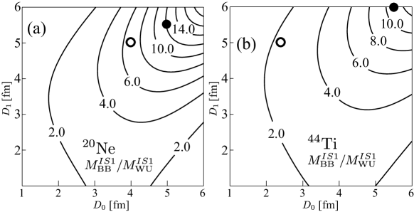
Figure 1: The ratio of the transition matrix to the Weisskopf estimate $M_{\rm BB}^{IS1}/M_{\rm WU}^{IS1}$ as function of the intercluster distances in the ground state ($D_{0}$) and in the $1^{-}$ state ($D_{1}$). The panel (a) is for $\alpha$+${}^{16}{\rm O}$ $({}^{20}{\rm Ne})$ system, while the panel (b) is for $\alpha$+${}^{40}{\rm Ca}$ $({}^{44}{\rm Ti})$ system. The circles show the approximate positions of the ground and the excited $1^{-}$ states obtained by the Brink-Bloch GCM (filled circles) and AMD (open circles) calculations given in the Sec. IV.

In both systems, we see that even for the small values of $D_{0}$ and $D_{1}$, $M_{\rm BB}^{IS1}$ is larger than the Weisskopf estimates. It is impressive that the matrix element is considerably amplified, as both of $D_{0}$ and $D_{1}$ increase.

By more detailed calculations explained in the next section, the position of the ground and $1^{-}$ states are estimated approximately at the open circles in Fig. 1. Therefore, the transition strength is indeed considerably amplified and regarded as a good probe for asymmetric clustering.

III Microscopic nuclear models

To provide realistic and reliable results for the IS dipole transition of ²⁰Ne and ⁴⁴Ti, we performed two microscopic nuclear model calculations which we explain in this section. The first is the Brink-Bloch GCM and the other is AMD. Brink-Bloch GCM can describe the intercluster motion properly. In addition to this, AMD can also describe the the polarization and distortion of clusters.

In both of theoretical models, the following microscopic $A$-body Hamiltonian is commonly used.

$${H}=\sum_{i=1}^{A}{t}(i)+\sum_{i<j}^{A}{v}_{n}(ij)+\sum_{i<j}^{Z}{v}_{C}(ij)-{t}_{\rm cm},$$ (27)

where the Gogny D1S interaction gogn91 is used as an effective nucleon-nucleon interaction $v_{n}$. Coulomb interaction $v_{C}$ is approximated by a sum of seven Gaussians. The center-of-mass kinetic energy ${t}_{\rm cm}$ is exactly removed.

III.1 Generator coordinate method
with Brink-Bloch wave function

The Brink-Bloch GCM uses Eq. (22) as the basis function and employs the intercluster distance $D$ as generator coordinate. The width parameter $\nu$ is so chosen to minimize the ground state energy, that is found to be $\nu=0.16$ and $0.12$ $\rm fm^{-2}$ for ²⁰Ne and ⁴⁴Ti, respectively. In the practical calculation, $D$ is discretized ranging from 1.0 to 12.0 $\rm fm$ with an interval of 0.5 $\rm fm$, that generates 23 basis functions $\Phi^{l\pi}_{\rm BB}(D_{i}),\ i=1,...,23$.

To describe the ground and $\alpha$+${}^{16}{\rm O}$ cluster states, the basis functions are superposed,

$$\Psi^{l\pi}_{Mp}=\sum_{i}g_{ip}\Phi^{l\pi}_{BB}(D_{i}),$$ (28)

By solving the following Griffin-Hill-Wheeler equation Hill53 ; Hill57 , we obtain the eigenenergy $E_{p}$ and the coefficients of the superposition $g_{ip}$.

$$\sum_{i^{\prime}}{H^{l\pi}_{ii^{\prime}}g_{i^{\prime}p}}=E^{l\pi}_{p}\sum_{i^{\prime}}{N^{l\pi}_{ii^{\prime}}g_{i^{\prime}p}},$$ (29)

$$H^{l\pi}_{ii^{\prime}}=\langle{\Phi^{l\pi}_{\rm BB}(D_{i})|\hat{H}|\Phi^{l\pi}_{\rm BB}(D_{i^{\prime}})}\rangle,$$ (30)

$$N^{l\pi}_{ii^{\prime}}=\langle{\Phi^{l\pi}_{\rm BB}(D_{i})|\Phi^{l\pi}_{\rm BB}(D_{i^{\prime}})}\rangle.$$ (31)

Using thus-obtained wave functions for the ground and excited $1^{-}$ states, the reduced matrix element given in Eq. (6) is directly calculated.

III.2 Antisymmetrized molecular dynamics

In the AMD model amd1 ; amd2 , each nucleon is represented by a localized Gaussian wave packet,

$$\varphi_{i}({\bm{r}}) =\exp\biggl{\{}-\sum_{\sigma=x,y,z}\nu_{\sigma}\Bigl{(}r_{\sigma}-\frac{Z_{i\sigma}}{\sqrt{\nu_{\sigma}}}\Bigr{)}^{2}\biggr{\}}\chi_{i}\xi_{i},$$ (32)

$$\chi_{i} =a_{i}\chi_{\uparrow}+b_{i}\chi_{\downarrow},\quad\xi_{i}={\rm proton}\ {\rm or}\ {\rm neutron},$$

where $\chi_{i}$ and $\xi_{i}$ represent spin and isospin wave functions. The intrinsic wave function is a Slater determinant of nucleon wave packets,

$$\Phi_{\rm int}={\mathcal{A}}\{\varphi_{1}\varphi_{2}...\varphi_{A}\}.$$ (33)

The parameters of the intrinsic wave function, ${\bm{Z}}_{i}$, $a_{i}$, $b_{i}$ and $\nu_{\sigma}$, are determined by the energy minimization explained below.

Before the energy minimization, the intrinsic wave function is projected to the eigenstate of the parity,

$$\Phi^{\pi} =\frac{1+\pi P_{x}}{2}\Phi_{\rm int},\quad\pi=\pm,$$ (34)

Then, the above-mentioned parameters are determined to minimize the expectation value of the Hamiltonian $\widetilde{E}$ that is defined as

$$\widetilde{E} =\frac{\langle\Phi^{\pi}|\hat{H}|\Phi^{\pi}\rangle}{\langle\Phi^{\pi}|\Phi^{\pi}\rangle}+V_{c},$$ (35)

$$V_{c} =v_{\beta}(\langle\beta\rangle-\beta_{0})^{2}+v_{\gamma}(\langle\gamma\rangle-\gamma_{0})^{2}.$$ (36)

Here the potential $V_{c}$ is added to impose the constraint on the quadrupole deformation of intrinsic wave function that is parameterized by $\braket{\beta}$ and $\braket{\gamma}$ as defined in Ref. Kim12 . The magnitudes of $v_{\beta}$ and $v_{\gamma}$ are chosen large enough so that $\braket{\beta},\braket{\gamma}$ are, after the energy minimization, equal to $\beta_{0},\gamma_{0}$. By the energy minimization, we obtain the optimized wave function $\Phi^{\pi}_{\rm int}(\beta_{0},\gamma_{0})$ for discretized sets of $(\beta_{0},\gamma_{0})$ on the triangular lattice in $\beta$-$\gamma$ plane. The lattice size is 0.05 and the calculation is performed up to $\beta=0.9$.

After the energy minimization, we project out an eigenstate of angular momentum and perform the GCM calculation by using quadrupole deformation parameters $\beta_{0},\gamma_{0}$ as the generator coordinates. We also included the Brink-Bloch wave functions $\Phi^{J\pi}_{\rm BB}(D_{i})$ as the basis functions of GCM. For simplicity, we denote by $\Phi_{i}$ this set of basis functions. Because the AMD wave function is not necessarily axially symmetric, non-zero values of $K$ quantum number and their mixing must be taken into account. Hence the equation for the angular momentum projection and Griffin-Hill-Wheeler equation are

$$\Phi^{J\pi}_{MKi}=\frac{2J+1}{8\pi^{2}}\int d\Omega D^{J*}_{MK}(\Omega)\hat{R}(\Omega)\Phi^{\pi}_{i},$$ (37)

and

$$\Psi^{J\pi}_{Mp}=\sum_{Ki}g_{Kip}\Phi^{J\pi}_{MKi},$$ (38)

$$\sum_{i^{\prime}K^{\prime}}{H^{J\pi}_{KiK^{\prime}i^{\prime}}g_{K^{\prime}i^{\prime}p}}=E^{J\pi}_{p}\sum_{i^{\prime}K^{\prime}}{N^{J\pi}_{KiK^{\prime}i^{\prime}}g_{K^{\prime}i^{\prime}p}},$$ (39)

$$H^{J\pi}_{KiK^{\prime}i^{\prime}}=\langle{\Phi^{J\pi}_{MKi}|\hat{H}|\Phi^{J\pi}_{MK^{\prime}i^{\prime}}}\rangle,$$ (40)

$$N^{J\pi}_{KiK^{\prime}i^{\prime}}=\langle{\Phi^{J\pi}_{MKi}|\Phi^{J\pi}_{MK^{\prime}i^{\prime}}}\rangle.$$ (41)

Using the wave function given in Eq. (38) the transition matrix element is calculated.

For a better understanding of the results presented in the next section, it is helpful to note the differences between the Brink-Bloch GCM and AMD. First, because nucleons are treated as independent wave packets, AMD is able to describe various non-cluster states as well as the cluster states, while Brink-Bloch GCM is not. Secondly, from the same reason, AMD is capable to describe the polarization and distortion of clusters. Finally, since the Brink-Bloch wave functions are also employed as the basis function, the AMD includes the Brink-Bloch GCM as a part of its model space. In short, in the AMD, the distortion of clusters and the coupling between the cluster states and non-cluster states are taken into account.

III.3 Projection of AMD wave function to Brink-Bloch wave function

As explained above, AMD wave function is admixture of the cluster and non-cluster wave functions. To identify the cluster state from AMD results, it is convenient to introduce an approximate projector to Brink-Bloch wave function,

$$P_{\rm BB}=\sum_{ij}\ket{\Phi^{J\pi}_{\rm BB}(D_{i})}(B^{-1})_{ij}\bra{\Phi^{J\pi}_{\rm BB}(D_{j})},$$ (42)

where $B^{-1}$ is the inverse of overlap matrix $B$ defined $B_{ij}=\braket{\Phi^{J\pi}_{\rm BB}(D_{i})}{\Phi^{J\pi}_{\rm BB}(D_{j})}$. With this projector, AMD wave function Eq. (38) is projected to Brink-Bloch wave function,

$$P_{\rm BB}\Psi_{Mp}^{J\pi}=\sum_{i}G_{i}\Phi^{J\pi}_{\rm BB}(D_{i}),$$ (43)

$$G_{i}=\sum_{j}(B^{-1})_{ij}\braket{\Phi_{\rm BB}^{J\pi}(D_{i})}{\Psi_{Mp}^{J\pi}}$$ (44)

By substituting Eq. (23), (24) and (25) into r.h.s of Eq. (43) and by comparing it with Eq. (4), we calculated the coefficient of superposition $f_{N_{0}+1}$ and $f_{N_{0}+3}$ given in Tab. 1. The projector is also used to evaluate the amount of the cluster component in the AMD wave function, that is defined as

$$S=\braket{\Psi^{J\pi}_{Mp}}{P_{\rm BB}}{\Psi^{J\pi}_{Mp}}.$$ (45)

When this value is sufficiently large, the excited state may be regarded as cluster state.

We also explain how we estimated the intercluster distances $D_{0}$ and $D_{1}$ which are shown by circles in Fig. 1. We calculate the overlap between the GCM wave functions $\Psi_{Mp}^{J\pi}$ for the ground and $1^{-}$ states and Brink-Bloch wave function $\Phi_{\rm BB}^{J\pi}(D_{i})$,

$$\frac{|\braket{\Psi_{Mp}^{J\pi}}{\Phi_{\rm BB}^{J\pi}(D_{i})}|^{2}}{\braket{\Phi_{\rm BB}^{J\pi}(D_{i})}{\Phi_{\rm BB}^{J\pi}(D_{i})}},$$

and regard the distance $D_{i}$ at which the overlap has its maximum as $D_{0}$ or $D_{1}$.

IV microscopic model calculations for isoscalar dipole transition

In this section, we discuss the IS dipole transitions in ${}^{20}{\rm Ne}$ and ${}^{44}{\rm Ti}$ studied by Brink-Bloch GCM and AMD. In Refs. Kim04 ; Tan04 ; Kim06 , the cluster and non-cluster states of ${}^{20}{\rm Ne}$ and ${}^{44}{\rm Ti}$ have already been discussed based on AMD calculation, and the reader is directed to those references for more detail. Here we focus on the $\alpha$+${}^{16}{\rm O}$ and $\alpha$+${}^{40}{\rm Ca}$ cluster states and discuss the IS dipole transitions from the ground state to those cluster states.

IV.1 $\bm{\alpha}+\bf{}^{16}{O}$ cluster states in ${}^{\bf 20}{\bf Ne}$

The $\alpha$+${}^{16}{\rm O}$ cluster states in ${}^{20}{\rm Ne}$ have been studied in detail by many authors Mat75 ; Hee76 ; Kru92 ; Buc75 ; Hee76 ; Fuj79 ; Kru92 ; Duf94 ; Tak96 ; Kim04 ; Tan04 ; Bo13 ; Zhou15 and well established.

Figure 2: (color online) The observed and calculated $\alpha$+${}^{16}{\rm O}$ cluster states in ${}^{20}{\rm Ne}$ classified into three rotational bands. Energy is measured from the $\alpha$ threshold located at 4.7 MeV above the ground state. In the AMD result, the $6^{+}$ member state of nodal excited band is fragmented into two states due to the coupling with non-cluster configurations.

The observed $\alpha$+${}^{16}{\rm O}$ cluster bands are summarized in Fig. 2 together with the results of Brink-Bloch GCM and AMD. The $0^{+}_{4}$ state observed at 8.7 MeV (4 MeV above the $\alpha$ threshold) has large $\alpha$ decay width comparable with the Wigner limit and is known as the nodal excited cluster state described by the wave function of Eq. (3). A rotational band is built on this state, which hereafter we call “nodal excited band”. The $1^{-}_{1}$ state at 5.8 MeV (1.1 MeV above the $\alpha$ threshold) also has large $\alpha$ decay width and is known as the angular excited cluster state described by the wave function of Eq. (4). This $1^{-}_{1}$ state is of particular importance because it is regarded as the evidence for the asymmetric clustering with $\alpha$+${}^{16}{\rm O}$ configuration. On this state, the negative-parity band is built.

It is well known that the ground band is the positive-parity partner of the negative-parity band, and those two bands constitute the parity doublet Hor68 . This means that the ground state has non-negligible cluster correlation. Therefore, on the basis of the discussion made in in Sec. II.2, we expect that the IS dipole transition to the $1^{-}_{1}$ state is considerably amplified.

Table 2: The estimated intercluster distance of the ground and the $\alpha$+${}^{16}{\rm O}$ cluster states in units of fm, and the IS dipole and monopole transition matrix from the ground state to the $1^{-}_{1}$ and $0^{+}_{4}$ states in units of $\rm fm^{3}$ and $\rm fm^{2}$. Numbers in parenthesis are ratio to the Weisskopf estimates.

	$D_{0}$	$D_{1}$	$D(0^{+}_{4})$	$M^{IS1}$	$M^{IS0}$
BB GCM	5.0	5.5	6.5	90.2 (10.7)	46.4 (7.3)
AMD	4.0	5.0	6.0	38.0 (4.5)	16.0 (2.5)

Then, we examine theoretical results. In the case of ${}^{20}{\rm Ne}$, it was easy to identify the $\alpha$+${}^{16}{\rm O}$ cluster states from AMD results, because all of the states shown in Fig. 2 have large values of $S$ defined in Eq. (45). For example, $S=0.69,0.90$ and 0.81 for the ground, $1^{-}_{1}$ and $0^{+}_{4}$ states.

It is interesting to note the difference between the Brink-Bloch GCM and AMD results. The Brink-Bloch GCM fails to reproduce the energy of the ground band, while AMD reasonably describes it, that indicates the importance of the cluster distortion effect. Indeed the estimated intercluster distance $D$ is reduced in AMD compared to Brink-Bloch GCM as listed in Tab. 2. On the other hand, both theoretical models give reasonable description for negative-parity and nodal excited bands. Therefore, we can regard that the distortion effect is less important and almost ideal clustering is realized in the $0^{+}_{4}$ and $1^{-}_{1}$ states, for which both theoretical models yielded large intercluster distances.

The calculated IS dipole transition matrix from the ground state to the $1^{-}$ states are listed in Tab. 2. It is evident that the transition is greatly enhanced compared to Weisskopf estimates. In particular, Brink-Bloch GCM yielded huge values, that is due to the too weak binding of the ground state leading to the overestimation of the radius and cluster correlation of the ground state. If the cluster distortion effect is taken into account by AMD, the strength is somewhat reduced but still much larger than the Weisskopf estimate. We also note that the nodal excited state ($0^{+}_{4}$) has large monopole transition matrix as expected. Therefore, the present results suggest that both of the positive- and negative-parity cluster states can be strongly generated by the IS monopole and dipole transitions from the ground state, and hence, those transitions will be good signature of the asymmetric clustering.

IV.2 $\bm{\alpha}+\bf{}^{40}{Ca}$ cluster states in ${}^{\bf 44}{\bf Ti}$

The $\alpha$+${}^{40}{\rm Ca}$ cluster states in ${}^{44}{\rm Ti}$ have also been studied by many authors Yam90 ; Yam93-2 ; Yam96 ; Yam93 ; Joh69 ; Str74 ; Fre75 ; Fre76 ; Fre83 ; Cha84 ; Mic86 ; Wad88 ; Ohk98 ; Kim06 , but the situation is more complicated than the case of ${}^{20}{\rm Ne}$. The theoretical and experimental studies are summarized in a review paper OhkR , and we discuss based on the assignment given therein.

Figure 3: (color online) The observed and calculated $\alpha$+${}^{40}{\rm Ca}$ cluster states in ${}^{44}{\rm Ti}$ classified into four rotational bands. Energy is measured from the $\alpha$ threshold located at 5.1 MeV above the ground state. In the experiment and AMD results, the member states of the nodal excited band and negative-parity band II are fragmented into several levels, and the weighted averages of those levels are shown in the figure.

Figure 3 shows the observed candidates of $\alpha$+${}^{40}{\rm Ca}$ cluster states together with the present theoretical results. Based on the $\alpha$ transfer experiment, four rotational bands including the ground band were classified as the $\alpha$+${}^{40}{\rm Ca}$ cluster bands. The $1^{-}$ state observed at 6.2 MeV (1.1 MeV above the $\alpha$ threshold) is strongly populated by the $\alpha$ transfer reaction Yam93 ; Yam93-2 and is the angular excited cluster state dominated by the 1$\hbar\omega$ excitation of the intercluster motion. Although it is not the yrast $1^{-}$ state, we call this state the $1^{-}_{1}$ state in the following. On this $1^{-}_{1}$ state, a rotational band which we call “negative-parity band I” is built.

A couple of candidates of the nodal excited $0^{+}$ state are reported around 11.0 MeV (5.9 MeV above the $\alpha$ threshold) by the $\alpha$ elastic scattering Fre83 and the $\alpha$ transfer reaction Yam90 ; Yam96 ; Yam93-2 . Those data suggest that the nodal excited cluster state may be fragmented into several states due to the coupling with other non-cluster configurations. In Fig. 3, by taking the average, the nodal excited state is plotted as a single state which we call the $0^{+}_{2}$ state. On this $0^{+}_{2}$ state the nodal excited band is built.

Around 12 MeV in excitation energy, another group of $1^{-}$ states having large $\alpha$ spectroscopic factors are reported Yam90 ; Yam93-2 ; Yam96 . Again, observed $\alpha$ spectroscopic factors are fragmented into several levels and the averaged value which we call the $1^{-}_{2}$ state is shown in the figure. Although the assignment is not so firm, another negative-parity band is suggested on this state which we denote by “negative-parity band II”. The excitation energy of this band plausibly agrees with the cluster model calculation which suggests the $3\hbar\omega$ excitation of the intercluster motion.

The information on the $\alpha$+${}^{40}{\rm Ca}$ cluster states is summarized as follows. First, the ground and the negative-parity band I built on the $1^{-}_{1}$ state at 6.2 MeV constitute a parity doublet. Second, the nodal excited band built on the $0^{+}_{2}$ state around 11 MeV and the negative-parity band II on the $1^{-}_{2}$ state around 12 MeV may constitute another parity doublet. The first doublet is dominated by the 0 and 1$\hbar\omega$ excitations of the intercluster motion, while the second doublet is dominated by the $2\hbar\omega$ and $3\hbar\omega$ excitations.

Table 3: The estimated intercluster distance of the ground and the $\alpha$+${}^{40}{\rm Ca}$ cluster states in units of fm, and the IS dipole and monopole transition matrix from the ground state to the $1^{-}_{1}$, $1^{-}_{2}$ and $0^{+}_{2}$ states in units of $\rm fm^{3}$ and $\rm fm^{2}$. Intercluster Distances $D(0^{+}_{2})$ and $D(1^{-}_{2})$ are the averaged values of the fragmented levels, while the transition matrix $M^{IS0}(0^{+}_{2})$ and $M^{IS1}(1^{-}_{2})$ are sum of them. Numbers in parenthesis are ratio to the Weisskopf estimates.

	$D_{0}$	$D_{1}$	$D(0^{+}_{2})$	$D(1^{-}_{2})$
BB GCM	5.5	6.0	7.0	7.5
AMD	2.5	5.0	6.0	7.0
	$M^{IS1}(1^{-}_{1})$	$M^{IS0}(0^{+}_{2})$	$M^{IS1}(1^{-}_{2})$
BB GCM	217.5 (11.7)	47.2 (4.4)	91.6 (4.9)
AMD	24.7 (1.3)	19.9 (1.8)	16.7 (0.9)

Next, we discuss the results of Brink-Bloch GCM. The Brink-Bloch GCM seriously overestimates the energies of the observed cluster bands as well as the ground band indicating the increased importance of the cluster distortion. Because of too weak binding, all states have large intercluster distances that result in the huge dipole and monopole transition matrix listed in Tab. 3 which may be overamplified and unrealistic.

In the AMD results, the member states of the nodal excited band and negative-parity band II are fragmented into several states as reported by the experiment. Therefore, for the states shown in Fig. 3 and the intercluster distances listed in Tab. 3, we show the averaged values weighted by the amount of the cluster component $S$ given by Eq. (45). By taking the distortion effect into account, AMD gives a reasonable description of the ground and cluster bands. All states gain large binding energy compared to the Brink-Bloch GCM, and their intercluster distances, in particular that of the ground state, are considerably reduced. This strong distortion is mainly due to the spin-orbit interaction and to the formation of the mean field.

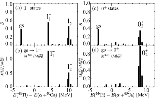
Figure 4: (a) The amount of the cluster component $S$ of the ground and $1^{-}$ states obtained by AMD. (b) The ratio of IS dipole transition matrix $M^{IS1}$ to the Weisskopf estimate. (c) Same as (a) but for the $0^{+}$ states. (d) Same as (b) but for the IS monopole transition.

Since the nodal excited band and negative-parity band II are fragmented, we discuss the transition matrix by referring the distribution of the amount of the cluster component $S$. Fig 4 (a) shows $S$ of the ground and $1^{-}$ states as function of energy relative to the $\alpha$ threshold. The ground state has, despite of the strong cluster distortion, considerable amount of cluster component $S=0.39$. However, we note that this does not necessarily mean the prominent clustering in the ground state. Most of this cluster component is the wave function given in Eq. (1) and hence identical to the shell model wave function. The first angular excited state (the $1^{-}_{1}$ state) located at 4 MeV above the threshold has larger value of $S=0.59$. The second angular excited state (the $1^{-}_{2}$ state) is fragmented into three levels around 10 MeV above the threshold. If we sum up those fragments, it amounts to $S=0.78$. The IS dipole transition matrix from the ground state to $1^{-}$ states are shown in Fig. 4 (b). It is clear that both of the angular excited states are strongly excited, because the IS dipole transition brings about 1 and 3$\hbar\omega$ excitation of the intercluster motion as shown by Eq. (14). It must be noted that many non-cluster $1^{-}$ states are obtained between the ground and $1^{-}_{2}$ states in AMD calculation, but none of them have the transition matrix comparable with Weisskopf estimate. This result shows that the IS dipole transition has the sensitivity to for angular excited $1^{-}$ states, despite of the cluster distortion and fragmentation.

As for the $0^{+}$ states and monopole transition, almost the same conclusion can be drawn. Fig. 4 (c) shows the amount of the cluster component in the $0^{+}$ states. Around 8 MeV, the nodal excited $0^{+}_{2}$ state is fragmented into three levels, which amount to $S=0.6$. Again, we see the amount of cluster component $S$ and transition matrix are strongly correlated. The nodal excited states have large IS monopole transition matrix, while non-cluster states are insensitive. From those results, we conclude that the IS monopole and dipole transitions are good probe for asymmetric clustering. Since both transitions can be measured simultaneously by the $\alpha$ inelastic scattering, the experimental and theoretical survey look promising.

We also comment on the giant resonances, which may exist at the similar energy region to the $1^{-}_{2}$ and $0^{+}_{2}$ states. Because the peak of giant resonance may overlap with those states, those nodal excited doublet may not be visible in the real situation. Nevertheless, we expect that it is possible to identify those cluster state, because those cluster states will dominantly decay by $\alpha$ emission, while the giant resonance decay by neutron emission.

V Summary

In this study, we have discussed the IS dipole transition in ${}^{20}{\rm Ne}$ and ${}^{44}{\rm Ti}$ that have $\alpha$+${}^{16}{\rm O}$ and $\alpha$+${}^{40}{\rm Ca}$ cluster states. In such asymmetric cluster systems, the existence of the angular excited $1^{-}$ cluster states is a key to prove their asymmetric structure. We have shown that the isoscalar dipole transition from the ground state strongly populates those asymmetric cluster states, and hence, it is regarded as a good probe for such $1^{-}$ states.

We first performed analytical calculations to estimate the magnitude of the transition matrix. By rewriting the IS dipole operator in terms of the internal coordinates within clusters and the intercluster coordinate, it was shown that the transition brings about the 1 and 3$\hbar\omega$ excitation to the intercluster motion. Therefore, the IS dipole transition has the potential to activate the degrees-of-freedom of cluster excitation embedded in the ground state to populate the angular excited $1^{-}$ cluster states.

By assuming that the ground state is described by a shell model wave function, we have derived an analytical expression of the IS transition matrix, and demonstrated that the transition matrix is indeed enhanced and is in the order of Weisskopf estimate, even if the ground state has an ideal shell model structure. We also performed a simple numerical calculation using Brink-Bloch wave function to show that the transition matrix is amplified in order of magnitude if the ground state has cluster correlation.

To provide realistic and reliable result for IS monopole and dipole transitions in ${}^{20}{\rm Ne}$ and ${}^{44}{\rm Ti}$, nuclear structure calculations using Brink-Bloch GCM and AMD were performed. By taking the cluster distortion into account, AMD reasonably described the energies of those cluster states. It was shown that despite of the cluster distortion, the nodal and angular excited cluster states are strongly excited by the IS monopole and dipole transitions, and hence, we conclude that the monopole and dipole transitions are promising probe for asymmetric clustering.

Appendix A IS dipole operator represented by internal and intercluster coordinates

We consider the $A$ nucleon system composed of the clusters with mass $C_{1}$ and $C_{2}$ ($C_{1}+C_{2}=A$), and wish to express $\mathcal{M}_{\mu}^{IS1}$ in terms of the internal coordinates $\bm{\xi}_{i}$ within each cluster and the intercluster coordinate $\bm{r}$. Noting the relations $\bm{R}_{C_{1}}-\bm{r}_{\rm cm}={C_{2}}/{A}\bm{r}$ and $\bm{R}_{C_{2}}-\bm{r}_{\rm cm}=-{C_{1}}/{A}\bm{r}$, the IS dipole operator is rewritten as follows,

$$\mathcal{M}_{\mu}^{IS1}= \sum_{i=1}^{A}(\bm{r}_{i}-\bm{r}_{\rm cm})^{2}\mathcal{Y}_{1\mu}(\bm{r}_{i}-\bm{r}_{\rm cm})$$

$$= \sum_{i\in C_{1}}\Bigl{(}\bm{\xi}_{i}+\frac{C_{2}}{A}\bm{r}\Bigr{)}^{2}\mathcal{Y}_{1\mu}\Bigl{(}\bm{\xi}_{i}+\frac{C_{2}}{A}\bm{r}\Bigr{)}+\sum_{i\in C_{2}}\Bigl{(}\bm{\xi}_{i}-\frac{C_{1}}{A}\bm{r}\Bigr{)}^{2}\mathcal{Y}_{1\mu}\Bigl{(}\bm{\xi}_{i}-\frac{C_{1}}{A}\bm{r}\Bigr{)}$$

$$= \sum_{i\in C_{1}}\xi_{i}^{2}\mathcal{Y}_{1\mu}(\bm{\xi}_{i})+\sum_{i\in C_{2}}\xi_{i}^{2}\mathcal{Y}_{1\mu}(\bm{\xi}_{i})+\left(\frac{C_{2}}{A}\sum_{i\in C_{1}}\xi_{i}^{2}-\frac{C_{1}}{A}\sum_{i\in C_{1}}\xi_{i}^{2}\right)\mathcal{Y}_{1\mu}(\bm{r})-\frac{C_{1}C_{2}(C_{1}-C_{2})}{A^{2}}r^{2}\mathcal{Y}_{1\mu}(\bm{r})$$

$$+2\frac{C_{2}}{A}\sum_{i\in C_{1}}(\bm{\xi}_{i}\cdot\bm{r})\mathcal{Y}_{1\mu}(\bm{\xi}_{i})-2\frac{C_{1}}{A}\sum_{i\in C_{2}}(\bm{\xi}_{i}\cdot\bm{r})\mathcal{Y}_{1\mu}(\bm{\xi}_{i}),$$ (46)

where the relations $\sum_{i\in C_{1}}\bm{\xi}_{i}=\sum_{i\in C_{2}}\bm{\xi}_{i}=0$ and $\mathcal{Y}_{1\mu}(\alpha\bm{a}+\beta\bm{b})=\alpha\mathcal{Y}_{1\mu}(\bm{a})+\beta\mathcal{Y}_{1\mu}(\bm{b})$ are utilized. Using the identities, $\bm{a}\cdot\bm{b}=-4\pi/\sqrt{3}[\mathcal{Y}_{1}(\bm{a})\otimes\mathcal{Y}_{1}(\bm{b})]_{00},\ \ [\mathcal{Y}_{1}(\bm{a})\otimes\mathcal{Y}_{1}(\bm{a})]_{1\mu}=0,\text{ and }[\mathcal{Y}_{1}(\bm{a})\otimes\mathcal{Y}_{1}(\bm{a})]_{2\mu}=\sqrt{3/10\pi}\mathcal{Y}_{2\mu}(\bm{a})$ the term in last line of Eq. (46) reads,

$$(\bm{\xi}_{i}\cdot\bm{r})\mathcal{Y}_{1\mu}(\bm{\xi}_{i})= -\frac{4\pi}{\sqrt{3}}[\mathcal{Y}_{1}(\bm{\xi}_{i})\otimes[\mathcal{Y}_{1}(\bm{\xi}_{i})\otimes\mathcal{Y}_{1}(\bm{r})]_{0}]_{1\mu}$$

$$= -\frac{4\pi}{\sqrt{3}}\sum_{l=0,1,2}\sqrt{2l+1}\left\{\begin{array}[]{ccc}1&1&l\\ 1&1&0\end{array}\right\}[[\mathcal{Y}_{1}(\bm{\xi}_{i})\otimes\mathcal{Y}_{1}(\bm{\xi}_{i})]_{l}\otimes\mathcal{Y}_{1}(\bm{r})]_{1\mu}$$ (49)

$$= \frac{1}{3}\bm{\xi}_{i}^{2}\mathcal{Y}_{1\mu}(\bm{r})-\sqrt{\frac{8\pi}{9}}[\mathcal{Y}_{2}(\bm{\xi}_{i})\otimes\mathcal{Y}_{1}(\bm{r})]_{1\mu}.$$ (50)

We see Eqs. (46) and (50) yield Eq. (14).

Appendix B Derivation of IS dipole matrix element

Here, we derive Eq. (15) from Eqs. (8) and (14) in a similar way to Ref. Yam08 . First, we show that the first line of Eq. (14) identically vanishes in the case of the system composed of two $LS$ closed shell (more strictly, $SU(3)$ scalar) clusters. This is easily proved by counting the principal quantum numbers.

For example, the first term of Eq. (14) yields the matrix element proportional to

$$\braket{\mathcal{R}_{N10}(\bm{r})\Bigl{(}\sum_{i\in C_{1}}\xi_{i}^{2}\mathcal{Y}_{10}(\bm{\xi}_{i})\phi_{1}\Bigr{)}\phi_{2}}{\mathcal{A}^{\prime}\Set{\mathcal{R}_{N_{0}00}(\bm{r})\phi_{1}\phi_{2}}}.$$

Denoting the principal quantum number of $\phi_{1},\phi_{2}$ as $N_{C_{1}},N_{C_{2}}$, the principal quantum number of the ket state is equal to $N_{0}+N_{C_{1}}+N_{C_{2}}$. On the other hand, that of the bra state is equal to or larger than $N+N_{C_{1}}+N_{C_{2}}+1$, because $\sum_{i\in C_{1}}\xi_{i}^{2}\mathcal{Y}_{10}(\bm{\xi}_{i})$ induces at least $1\hbar\omega$ excitation of $\phi_{1}$. Since $N$ is equal to or larger than $N_{0}+1$, the principal quantum number of bra state is larger than that of ket state, and hence, this matrix element vanishes. In the same way, the third term of the first line yields

$$\langle\mathcal{R}_{N10}(\bm{r})\mathcal{Y}_{1m}(\bm{r})\Bigl{(}\sum_{i\in C_{1}}\mathcal{Y}_{2-m}(\bm{\xi}_{i})\phi_{1}\Bigr{)}\phi_{2}|\mathcal{A}^{\prime}\{\mathcal{R}_{N_{0}00}(\bm{r})\phi_{1}\phi_{2}\}\rangle.$$ (51)

The quantum number of $\sum_{i\in C_{1}}\mathcal{Y}_{2-m}(\bm{\xi}_{i})\phi_{1}$ is at least $N_{C_{1}}+2$, because $\sum_{i\in C_{1}}\mathcal{Y}_{2-m}(\bm{\xi}_{i})$ generates $2^{+}$ states of the $LS$ closed shell nucleus $\phi_{1}$ which involves at least $2\hbar\omega$ excitation. Combined with the quantum number of the intercluster motion which is at least $N-1$, we again find the quantum number of the bra state is larger than that of the ket state. Thus, terms that involve the internal cluster excitation vanish.

However, for the open-shell (non $SU(3)$ scalar) clusters, it must be noted that Eq. (51) do not vanish and can be very large. A typical example is ¹²C cluster. For such clusters, the wave function in the parenthesis in Eq. (51) is written as

$$\sum_{i\in{\rm{}^{12}C}}\mathcal{Y}_{2-m}(\bm{\xi}_{i})\phi_{\rm{}^{12}C}(0^{+}_{1})=\braket{\phi_{\rm{}^{12}C}(2^{+}_{1})}{\sum_{i\in\rm^{12}C}\mathcal{Y}_{2-m}(\bm{\xi}_{i})}{\phi_{\rm{}^{12}C}(0^{+}_{1})}\phi_{\rm{}^{12}C}(2^{+}_{1})+(\text{other excited $2^{+}$ states}).$$ (52)

Since $\phi_{\rm{}^{12}C}(2^{+}_{1})$ has the same principal quantum number with the ground state $\phi_{\rm{}^{12}C}(0^{+}_{1})$ and the matrix element $\braket{\phi_{\rm{}^{12}C}(2^{+}_{1})}{\sum_{i\in\rm^{12}C}\mathcal{Y}_{2-m}(\bm{\xi}_{i})}{\phi_{\rm{}^{12}C}(0^{+}_{1})}$ is proportional to large $E2$ matrix element, Eq. (51) can be comparable or even larger than the second line of Eq. (14). We conclude that if the cluster nucleus has the rotational or vibrational ground band with enhanced $E2$ transition, the internal excitation of the cluster from $0^{+}$ to $2^{+}$ can have large contribution to IS dipole excitation.

Now we evaluate the non-vanishing contribution from the second line. The first term of the second line yields the the matrix element proportional to

$$\braket{\mathcal{R}_{N10}(\bm{r})\mathcal{Y}_{10}(\bm{r})\Bigl{(}\sum_{i\in C_{1}}\mathcal{\bm{missing}}\xi_{i}^{2}\phi_{1}\Bigr{)}\phi_{2}}{\mathcal{A}^{\prime}\Set{\mathcal{R}_{N_{0}00}(\bm{r})\phi_{1}\phi_{2}}}.$$ (53)

Note that, in the bra state, the IS monopole operator $\sum_{i\in C_{1}}\xi_{i}^{2}$ induces 0 or $2\hbar\omega$ excitation of $\phi_{C_{1}}$,

$$\sum_{i\in C_{1}}\mathcal{\bm{missing}}\xi_{i}^{2}\phi_{1}= \braket{\phi_{1}}{\sum_{i\in C_{1}}\mathcal{\bm{missing}}\xi_{i}^{2}}{\phi_{1}}\phi_{1}+(\text{$2\hbar\omega$ excited $0^{+}$ states}).$$ (54)

and $\mathcal{Y}_{10}(\bm{r})$ brings about the angular excitation of the intercluster motion with $\pm 1\hbar\omega$, i.e., the principal quantum number of the intercluster motion is equal to $N\pm 1$. Again we count the quantum numbers and find that Eq. (53) is non zero only when $N=N_{0}+1$, otherwise the principal quantum number of the bra state is larger than that of the ket state. From Eq. (54) and the following identities,

$$\mathcal{R}_{N10}(\bm{r})\mathcal{Y}_{1m}(\bm{r})=\sqrt{\frac{1}{4\pi}}rR_{N1}(r)Y_{00}(\hat{r})+\sqrt{\frac{1}{5\pi}}rR_{N1}(r)Y_{20}(\hat{r}),$$ (55)

$$rR_{N1}(r)=\sum_{N^{\prime}}\braket{R_{N^{\prime}0}}{r}{R_{N1}}R_{N^{\prime}0}(r),$$ (56)

Eq. (53) is calculated as,

$$\sqrt{\frac{1}{4\pi}}\braket{\phi_{1}}{\sum_{i\in C_{1}}\mathcal{\bm{missing}}\xi_{i}^{2}}{\phi_{1}}\sum_{N^{\prime}}\braket{R_{N^{\prime}0}}{r}{R_{N_{0}+11}}\braket{R_{N^{\prime}0}(r)Y_{00}(\hat{r})\phi_{1}\phi_{2}}{\mathcal{A}^{\prime}\Set{R_{N_{0}0}(r)Y_{00}(\hat{r})\phi_{1}\phi_{2}}}$$

$$=\sqrt{\frac{1}{4\pi}}C_{1}\braket{r_{C_{1}}^{2}}\braket{R_{N_{0}0}}{r}{R_{N_{0}+11}}\mu_{N_{0}},$$ (57)

where $\braket{r^{2}}_{C_{1}}$ is the square of the root-mean-square radius of $\phi_{C_{1}}$.

Finally, the last term in the second line of Eq. (14) yields

$$\braket{\mathcal{R}_{N10}(\bm{r})r^{2}\mathcal{Y}_{10}(\bm{r})\phi_{1}\phi_{2}}{\mathcal{A}^{\prime}\Set{\mathcal{R}_{N_{0}00}(\bm{r})\phi_{1}\phi_{2}}},$$ (58)

where $r^{2}\mathcal{Y}_{10}(\bm{r})$ brings about the nodal and angular excitations of the intercluster motion with $\pm 1\hbar\omega$ or $\pm 3\hbar\omega$, and hence the matrix element vanishes except for $N=N_{0}+1$ and $N_{0}+3$ cases. By a similar calculation, one finds Eq. (58) is equal to

$$\sqrt{\frac{1}{4\pi}}\braket{R_{N_{0}0}}{r^{3}}{R_{N1}}\mu_{N_{0}},$$ (59)

where $N$ is $N_{0}+1$ or $N_{0}+3$. From those results, we obtain an analytic expression for the reduced matrix element given in Eq. (14).

Appendix C Sign of $\bm{f}_{\bm{N}_{0}\bf+1}$ and $f_{\bm{N}_{0}\bf+3}$

The coefficients $f_{N_{0}+1}$ and $f_{N_{0}+3}$ in Eq. (4) usually have opposite sign for cluster states. To show it, we first approximate the wave function of angular excited cluster state Eq. (4) as Brink-Bloch wave function given in Eq. (22) and (23). This approximation may be justified, because those wave functions have large overlap to each other with proper choice of $R$. For example, in the case of ${}^{20}{\rm Ne}$, the overlap between the Brink-Bloch wave function with $R=5.0$ fm and the AMD wave function for the $1^{-}_{1}$ state amounts to 82%.

Given that the approximation is reasonable, substitute Eq. (24) to Eq. (23) and compare it with Eq. (4). As a result, one finds the sign of $f_{N}$ is equal to that of $A_{Nl}$ defined by Eq. (25). Therefore, $f_{N_{0}+1}$ and $f_{N_{0}+3}$ should have opposite sign, if the angular excited state is well approximated by Brink-Bloch wave function.

References

- (1) D. H. Youngblood, Y.-W. Lui, and H. L. Clark, Phys. Rev. C 55, 2811 (1997).
- (2) D. H. Youngblood, Y.-W. Lui, and H. L. Clark, Phys. Rev. C 57, 2748 (1998).
- (3) D. H. Youngblood, Y.-W. Lui, and H. L. Clark, Phys. Rev. C 60, 014304 (1998).
- (4) Y. -W. Lui, H. L. Clark, and D. H. Youngblood, Phys. Rev. C 64, 064308 (2001).
- (5) D. H. Youngblood, Y.-W. Lui, and H. L. Clark, Phys. Rev. C 65, 034302 (2002).
- (6) B. John, Y. Tokimoto, Y. -W. Lui, H. L. Clark, X. Chen, and D. H. Youngblood, Phys. Rev. C 68, 014305 (2003).
- (7) D. H. Youngblood, Y.-W. Lui, and H. L. Clark, Phys. Rev. C 76, 027304 (2007).
- (8) T. Wakasa et al., Phys. Lett. B 653, 173 (2007).
- (9) T. Kawabata et al., Int. J. Mod. Phys. E 17, 2071 (2008).
- (10) D. H. Youngblood, Y. -W. Lui, X. F. Chen, and H. L. Clark, Phys. Rev. C 80, 064318 (2009).
- (11) X. Chen, Y. -W. Lui, H. L. Clark, Y. Tokimoto, D. H. Youngblood, Phys. Rev. C 80, 014312 (2009).
- (12) M. Itoh et al., Phys. Rev. C 84, 054308 (2011).
- (13) M. R. Anders, S. Shlomo, T. Sil, D. H. Youngblood, Y. -W. Lui, and Krishichayan, Phys. Rev. C 87, 024303 (2013).
- (14) Y. K. Gupta et al., Phys. Lett. B 748, 343 (2015).
- (15) E. Uegaki, S. Okabe, Y. Abe, and H. Tanaka, Prog. Theor. Phys. 57, 1262 (1977).
- (16) E. Uegaki, Y. Abe, S. Okabe, and H. Tanaka, Prog. Theor. Phys. 62, 1621 (1979).
- (17) M. Kamimura, Nucl. Phys. A 351, 456 (1981).
- (18) P. Descouvemont, and D. Baye, Phys. Rev. C 36, 54 (1987).
- (19) Y. Kanada-En’yo, Phys. Rev. Lett. 81, 5291 (1998).
- (20) A. Tohsaki, H. Horiuchi, P. Schuck, and G. Röpke, Phys. Rev. Lett. 87, 192501 (2001).
- (21) Y. Funaki, A. Tohsaki, H. Horiuchi, P. Schuck, and G. Röpke, Phys. Rev. C 67, 051306 (2003).
- (22) T. Neff, and H. Feldmeier, Nucl. Phys. A 738, 357 (2004).
- (23) Y. Funaki, A. Tohsaki, H. Horiuchi, P. Schuck, and G. Röpke, Eur. Phys. J A 28, 259 (2006).
- (24) M. Chernykh, H. Feldmeier, T. Neff. P. von Neumann-Cosel, and A. Richter, Phys. Rev. Lett. 98 032501 (2007).
- (25) Y. Suzuki, and S. Hara, Phys. Rev. C 39, 658 (1989).
- (26) T. Yamada, T. Myo, H. Horiuchi, K. Ikeda, G. Röpke, P. Schuck, and A. Tohsaki, Phys. Rev. C 85, 034315 (2012).
- (27) Y. Suzuki, Nucl. Phys. A 470, 119 (1987).
- (28) Y. Kanada-En’yo, Phys. Rev. C 75, 024302 (2007).
- (29) T. Kawabata et al., Phys. Lett. B 646, 6 (2007).
- (30) T. Yamada, and Y. Funaki, Phys. Rev. C 82, 064315 (2010).
- (31) T. Yamada, Y. Funaki, H. Horiuchi, K. Ikeda, and A. Tohsaki, Prog. Theor. Phys. 120, 1139 (2008).
- (32) B. F. Bayman, and A. Bohr, Nucl. Phys. 9, 596 (1958/1959).
- (33) T. Ichikawa, N. Itagaki, T. Kawabata, Tz. Kokalova, W. von Oertzen, Phys. Rev. C 83, 061301 (2011).
- (34) M. Ito, Phys. Rev. C 83, 044319 (2011).
- (35) M. Itoh et al., Phys. Rev. C 88, 064313 (2013).
- (36) T. Kawabata et al., Jour. Phys. Conf. Ser. 436, 012009 (2013).
- (37) Y.Kanada-En’yo, Phys. Rev. C 89, 024302 (2014).
- (38) Z. H. Yang et al., Phys. Rev. Lett. 112, 162501 (2014).
- (39) Z. H. Yang et al., Phys. Rev. C 91, 024304 (2015).
- (40) Y. Chiba, and M. Kimura, Phys. Rev. C 91, 061302 (2015).
- (41) H. Horiuchi, and K. Ikeda, Prog. Theor. Phys. 40, 277 (1968).
- (42) F. Iachello, Phys. Lett. B 160, 1 (1985).
- (43) Y. Alhassid, M. Gai,, and G. F. Bertsch, Phys. Rev. Lett. 49, 1482 (1982).
- (44) M. Gai, M. Ruscev, A. C. Hayes, J. F. Ennis, R. Keddy, E. C. Schloemer, S. M. Sterbenz, D. A. Bromley, Phys. Rev. Lett. 50, 239 (1983).
- (45) V. Z. Goldberg, K.-M. Källman, T. Lönnroth, P. Manngard and B. B. Skorodumov, Phys. At. Nucl. 68, 1079 (2005).
- (46) N. Curtis, D. D. Caussyn, C. Chandler, M. W. Cooper, N. R. Fletcher, R. W. Laird and J. Pavan, Phys. Rev. C 66, 024315 (2002).
- (47) N. I. Ashwood et al., J. of Phys. G 32, 463 (2006).
- (48) S. Yildiz, M. Freer, N. Soi Lc, S. Ahmed, N. I. Ashwood, N. M. Clarke, N. Curtis, B. R. Fulton, C. J. Metelko, B. Novatski, N. A. Orr, R. Pitkin, S. Sakuta and V. A. Ziman, Phys. Rev. C 73, 034601 (2006).
- (49) H. Daley, and F. Iachello, Phys. Lett. B 131, 281 (1983).
- (50) M. Gai, J. F. Ennis, M. Ruscev, E. C. Schloemer, B. Shivakumar, S. M. Sterbenz, N. Tsoupas,, and D. A. Bromley, Phys. Rev. Lett. 51, 646 (1983).
- (51) M. Gai, J. F. Ennis, D. A. Bromley, H. Emling, F. Azgui, E. Grosse, H. J. Wollersheim, C. Mittag, and F. Riess, Phys. Lett. B 215, 242 (1988).
- (52) A. Astier, P. Petkov, M. -G. Porquet, D. S. Delion,, and P. Schuck, Phys. Rev. Lett. 104, 042701 (2010).
- (53) Y. Suzuki, and S. Ohkubo, Phys.Rev. C 82, 041303 (2010).
- (54) D. S. Delion, R. J. Liotta, P. Schuck, A. Astier, and M. -G. Porquet, Phys. Rev. C 85, 064306 (2012).
- (55) M. Spieker, S. Pascu, A. Zilges, and F. Iachello, Phys. Rev. Lett. 114, 192504 (2015).
- (56) Y. Kanada-En’yo, arXiv:1512.03619 [nucl-th].
- (57) D. M. Brink, Proc. Int. School of Physics Enrico Fermi, Course 36, Varenna, ed. C. Bloch (Academic Press, New York, 1966).
- (58) Y. Kanada-En’yo, M. Kimura and H. Horiuchi, C. R. Physique 4, (2003) 497.
- (59) Y. Kanada-En’yo, M. Kimura and A. Ono, PTEP 2012, (2012) 01A202.
- (60) M. Harvey, and T. Sebe, Nucl. Phys. A 136, 459 (1969).
- (61) T. Tomoda, and A. Arima, Nucl. Phys. A 303, 217 (1978).
- (62) C. Vargas, J. G. Hirsch, P. O. Hess, and J. P. Draayer, Phys. Rev. C 58, 1488 (1998).
- (63) K. H. Bhatt and J. B. McGrory, Phys. Rev. C 3, 2293 (1971).
- (64) J. B.McGrory, Phys. Lett. B 47, 481 (1973).
- (65) A. Poves and A. Zuker, Phys. Rep. 70, 235 (1981).
- (66) J. P. Elliott, Proc. R. Soc. London A 245, 562 (1958).
- (67) D. R. Tilleya, C. M. Chevesa, J. H. Kelleya, S. Ramand, and H. R. Wellera, Nucl. Phys. A 636, 249 (1998).
- (68) T. Yamaya, S. Oh-ami, O. Satoh, M. Fujiwara, T. Itahashi, K. Katori, S. Kato, M. Tosaki, S. Hatori, S. Ohkubo, Phys. Rev. C 41, 2421 (1990).
- (69) T. Yamaya, S. Oh-ami, M. Fujiwara, T. Itahashi, K. Katori, M. Tosaki, S. Kato, S. Hatori, S. Ohkubo, Phys. Rev. C 42, 1935 (1990).
- (70) T. Yamaya, K. Ishigaki, H. Ishiyama, T. Suehiro, S. Kato, M. Fujiwara, K. Katori, M. H.Tanaka, S. Kubono, V. Guimaraes, S. Ohkubo, Phys. Rev. C 53, 131 (1996).
- (71) T. Yamaya, S. Ohkubo, S. Okabe, M. Fujiwara, Phys. Rev. C47, 2389 (1993).
- (72) I. Angelia, and K.P. Marinovab, Atomic data and Nucl. Data Tables, 99, 69 (2013).
- (73) H. Horiuchi, Prog. Theor. Phys. Suppl. 62, 90 (1977).
- (74) J. F. Berger, M. Girod, and D. Gogny, Comput. Phys. Comm. 63 (1991) 365.
- (75) D. L. Hill and J. A. Wheeler, Phys. Rev. 89, 112 (1953).
- (76) J. J. Griffin and J. A. Vfheeler, Phys. Rev. 108, 311 (1957).
- (77) M. Kimura, R. Yoshida, and M. Isaka, Prog. Theor. Phys. 127, 287 (2012).
- (78) M. Kimura, Phys. Rev. C 69, 044319 (2004).
- (79) Y. Taniguchi, M. Kimura, and H. Horiuchi, Prog. Theor. Phys. 112, 475 (2004).
- (80) M.Kimura, and H.Horiuchi, Nucl. Phys. A 767, 58 (2006).
- (81) T. Matsuse, M. Kamimura, and Y. Fukushima, Prog. Theor. Phys. 53, 706 (1975).
- (82) B. Buck, C. B. Dover, and J. -P. Vary, Phys. Rev. C 11, 1803 (1975).
- (83) P. -H. Heenen, Nucl. Phys. A 272, 399 (1976).
- (84) Y. Fujiwara, H. Horiuchi, and R. Tamagaki, Prog. Theor. Phys. 62, 122 (1979).
- (85) M. Kruglanski and D. Baye, Nucl. Phys. A 548, 39 (1992).
- (86) M. Dufour. P. Descouvemont, and D. Baye, Phys. Rev. C 50, 795 (1994).
- (87) S. Takami, K. Yabana, and K. Ikeda, Prog. Theor. Phys. 96, 407 (1996).
- (88) B. Zhou, Y. Funaki, H. Horiuchi, Z. Ren, G. Röpke, P. Schuck, A. Tohsaki, C. Xu, and T. Yamada, Phys. Rev. Lett. 110, 262501 (2013).
- (89) E. F. Zhou, J. M. Yao, Z. P. Li, J. Meng, P. Ring, Phys. Lett. B, in print.
- (90) J. John, C. P. Robinson, J. P. Aldridge and R. H. Davis, Phys. Rev. 177, 1755 (1969).
- (91) U. Strohbusch, C. L. Fink, B. Zeidman, R. G. Markham, H. W. Fulbright, and R. N. Horoshko, Phys. Rev. C 9, 965 (1974).
- (92) H. Friedrich and K. Langanke, Nucl. Phys. A252, 47 (1975).
- (93) D. Frekers, H. Eickhoff, H. Löhner, K. Poppensieker, R. Santo andC. Wiezorek, Z. Phys. A 276, 317 (1976).
- (94) D. Frekers, R. Santo and K. Langanke, Nucl. Phys. A 394, 189 (1983).
- (95) A. Chatterjee, S. Kailas, S. Saini, S. K. Gupta and M. K. Mehta, Z. Phys. A 317, 209 (1984).
- (96) F. Michel, G. Reidemeister, and S. Ohkubo, Phys. Rev. Lett. 57, 1215 (1986).
- (97) T. Wada, H. Horiuchi, Phys. Rev. C 38, 2063 (1988).
- (98) S.Ohkubo, Y.Hirabayashi, T.Sakuda, Phys. Rev. C 57, 2760 (1998).
- (99) F. Michel, S. Ohkubo and G. Reidmeister, Prog. Theor. Phys. Suppl 132, 7 (1998); T. Yamaya, K Katori, M. Fujiwara, S. Kato, and S. Ohkubo, ibid. 132, 73 (1998); T. Sakuda and S. Ohkubo, ibid. 132, 103 (1998).