New Perspectives on $k$-Support and Cluster Norms

Abstract

We study a regularizer which is defined as a parameterized infimum of quadratics, and which we call the box-norm. We show that the $k$-support norm, a regularizer proposed by Argyriou et al. (2012) for sparse vector prediction problems, belongs to this family, and the box-norm can be generated as a perturbation of the former. We derive an improved algorithm to compute the proximity operator of the squared box-norm, and we provide a method to compute the norm. We extend the norms to matrices, introducing the spectral $k$-support norm and spectral box-norm. We note that the spectral box-norm is essentially equivalent to the cluster norm, a multitask learning regularizer introduced by Jacob et al. (2009a), and which in turn can be interpreted as a perturbation of the spectral $k$-support norm. Centering the norm is important for multitask learning and we also provide a method to use centered versions of the norms as regularizers. Numerical experiments indicate that the spectral $k$-support and box-norms and their centered variants provide state of the art performance in matrix completion and multitask learning problems respectively.

Keywords: Convex Optimization, Matrix Completion, Multitask Learning, Spectral Regularization, Structured Sparsity.

1 Introduction

We continue the study of a family of norms which are obtained by taking the infimum of a class of quadratic functions. These norms can be used as a regularizer in linear regression learning problems, where the parameter set can be tailored to assumptions on the underlying regression model. This family of norms is sufficiently rich to encompass regularizers such as the $\ell_{p}$ norms, the group Lasso with overlap (Jacob et al., 2009b) and the norm of Micchelli et al. (2013). In this paper we focus on a particular norm in this framework – the box-norm – in which the parameter set involves box constraints and a linear constraint. We study the norm in detail and show that it can be generated as a perturbation of the $k$-support norm introduced by Argyriou et al. (2012) for sparse vector estimation, which hence can be seen as a special case of the box-norm. Furthermore, our variational framework allows us to study efficient algorithms to compute the norms and the proximity operator of the square of the norms.

Another main goal of this paper is to extend the $k$-support and box-norms to a matrix setting. We observe that both norms are symmetric gauge functions, hence by applying them to the spectrum of a matrix we obtain two orthogonally invariant matrix norms. In addition, we observe that the spectral box-norm is essentially equivalent to the cluster norm introduced by Jacob et al. (2009a) for multitask clustering, which in turn can be interpreted as a perturbation of the spectral $k$-support norm.

The characteristic properties of the vector norms translate in a natural manner to matrices. In particular, the unit ball of spectral $k$-support norm is the convex hull of the set of matrices of rank no greater than $k$, and Frobenius norm bounded by one. In numerical experiments we present empirical evidence on the strong performance of the spectral $k$-support norm in low rank matrix completion and multitask learning problems.

Moreover, our computation of the vector box-norm and its proximity operator extends naturally to the spectral case, which allows us to use proximal gradient methods to solve regularization problems using the cluster norm. Finally, we provide a method to use the centered versions of the penalties, which are important in applications (see e.g. Evgeniou et al., 2007; Jacob et al., 2009a).

1.1 Related Work

Our work builds upon a recent line of papers which considered convex regularizers defined as an infimum problem over a parametric family of quadratics, as well as related infimal convolution problems (see Jacob et al., 2009b; Bach et al., 2011; Maurer and Pontil, 2012; Micchelli and Pontil, 2005; Obozinski and Bach, 2012, and references therein). Related variational formulations for the Lasso have also been discussed in (Grandvalet, 1998) and further studied in (Szafranski et al., 2007).

To our knowledge, the box-norm was first suggested by Jacob et al. (2009a) and used as a symmetric gauge function in matrix learning problems. The induced orthogonally invariant matrix norm is named the cluster norm in (Jacob et al., 2009a) and was motivated as a convex relaxation of a multitask clustering problem. Here we formally prove that the cluster norm is indeed an orthogonal invariant norm. More importantly, we explicitly compute the norm and its proximity operator.

A key observation of this paper is the link between the box-norm and the $k$-support norm and in turn the link between the cluster norm and the spectral $k$-support norm. The $k$-support norm was proposed in (Argyriou et al., 2012) for sparse vector prediction and was shown to empirically outperform the Lasso (Tibshirani, 1996) and Elastic Net (Zou and Hastie, 2005) penalties. See also Gkirtzou et al. (2013) for further empirical results.

In recent years there has been a great deal of interest in the problem of learning a low rank matrix from a set of linear measurements. A widely studied and successful instance of this problem arises in the context of matrix completion or collaborative filtering, in which we want to recover a low rank (or approximately low rank) matrix from a small sample of its entries, see e.g. Srebro et al. (2005); Abernethy et al. (2009) and references therein. One prominent method of solving this problem is trace norm regularization: we look for a matrix which closely fits the observed entries and has a small trace norm (sum of singular values) (Jaggi and Sulovsky, 2010; Toh and Yun, 2011; Mazumder et al., 2010). In our numerical experiments we consider the spectral $k$-support norm and spectral box-norm as alternatives to the trace norm and compare their performance.

Another application of matrix learning is multitask learning. In this framework a number of tasks, such as classifiers or regressors, are learned by taking advantage of commonalities between them. This can improve upon learning the tasks separately, for instance when insufficient data is available to solve each task in isolation (see e.g. Evgeniou et al., 2005; Argyriou et al., 2007, 2008; Jacob et al., 2009a; Cavallanti et al., 2010; Maurer, 2006; Maurer and Pontil, 2008). An approach which has been successful is the use of spectral regularizers such as the trace norm to learn a matrix where the columns represent the individual tasks, and in this paper we compare the performance of the spectral $k$-support and box-norms as penalties in multitask learning problems.

Finally, we note that this is a longer version of the conference paper (McDonald et al., 2014) and includes new theoretical and experimental results.

1.2 Contributions

We summarise the main contributions of this paper.

• We show that the vector $k$-support norm is a special case of the more general box-norm, which in turn can be seen as a perturbation of the former. The box-norm can be written as a parameterized infimum of quadratics, and this framework is instrumental in deriving a fast algorithm to compute the norm and the proximity operator of the squared norm in $\mathcal{O}(d\log d)$ time. Apart from improving on the $\mathcal{O}(d(k+\log d))$ algorithm for the proximity operator in Argyriou et al. (2012), this method allows one to use optimal first order optimization algorithms (Nesterov, 2007) for the box-norm.

• We extend the $k$-support and box-norms to orthogonally invariant matrix norms. We note that the spectral box-norm is essentially equivalent to the cluster norm, which in turn can be interpreted as a perturbation of the spectral $k$-support norm in the sense of the Moreau envelope. Our computation of the vector box-norm and its proximity operator also extends naturally to the spectral case. This allows us to use proximal gradient methods for the cluster norm. Furthermore, we provide a method to apply the centered versions of the penalties, which are important in applications.

• We present extensive numerical experiments on both synthetic and real matrix learning datasets. Our findings indicate that regularization with the spectral $k$-support and box-norms produces state-of-the art results on a number of popular matrix completion benchmarks and centered variants of the norms show a significant improvement in performance over the centered trace norm and the matrix elastic net on multitask learning benchmarks.

1.3 Notation

We use ${{\mathbb{N}}}_{n}$ for the set of integers from $1$ up to and including $n$. We let ${\mathbb{R}}^{d}$ be the $d$ dimensional real vector space, whose elements are denoted by lower case letters. We let ${\mathbb{R}}^{d}_{+}$ and ${\mathbb{R}}^{d}_{++}$ be the subsets of vectors with nonnegative and strictly positive components, respectively. We denote by $\Delta^{d}$ the unit $d$-simplex, $\Delta^{d}=\{\lambda\in{\mathbb{R}}^{d+1}:\sum_{i=1}^{d+1}\lambda_{i}=1\}$. For any vector $w\in{\mathbb{R}}^{d}$, its support is defined as $\textrm{supp}(w)=\{i:w_{i}\neq 0\}\subseteq{{\mathbb{N}}}_{d}$. We use $1$ to denote either the scalar or a vector of all ones, whose dimension is determined by its context. Given a subset $g$ of ${{\mathbb{N}}}_{d}$, the $d$-dimensional vector $1_{g}$ has ones on the support $g$, and zeros elsewhere. We let ${\mathbb{R}}^{d\times T}$ be the space of $d\times T$ real matrices and write $W=[w_{1},\ldots,w_{T}]$ to denote the matrix whose columns are formed by the vectors $w_{1},\ldots,w_{T}\in{\mathbb{R}}^{d}$. For a vector $\sigma\in{\mathbb{R}}^{d}$, we denote by $\textrm{diag}(\sigma)$ the $d\times d$ diagonal matrix having elements $\sigma_{i}$ on the diagonal. We say matrix $W\in{\mathbb{R}}^{d\times T}$ is diagonal if $W_{ij}=0$ whenever $i\neq j$. We denote the trace of a matrix $W$ by ${\rm tr}(W)$, and its rank by $\textrm{rank}(W)$. We let $\sigma(W)\in{\mathbb{R}}_{+}^{r}$ be the vector formed by the singular values of $W$, where $r=\min(d,T)$, and where we assume that the singular values are ordered nonincreasing, i.e. $\sigma_{1}(W)\geq\ldots\geq\sigma_{r}(W)\geq 0$. We use ${\bf S}^{d}$ to denote the set of real $d\times d$ symmetric matrices, and ${\bf S}^{d}_{+}$ to denote the subset of positive semidefinite matrices. We use $\succeq$ to denote the positive semidefinite ordering on ${\bf S}^{d}$. The notation $\langle\cdot,\cdot\rangle$ denotes the standard inner products on ${\mathbb{R}}^{d}$ and ${\mathbb{R}}^{d\times T}$, that is $\langle x,y\rangle=\sum_{i=1}^{d}x_{i}y_{i}$ for $x,y\in{\mathbb{R}}^{d}$, and $\langle X,Y\rangle={\rm tr}(X^{\scriptscriptstyle\top}Y)$, for $X,Y\in{\mathbb{R}}^{d\times T}$. Given a norm $\|\cdot\|$ on ${\mathbb{R}}^{d}$ or ${\mathbb{R}}^{d\times T}$, $\|\cdot\|_{*}$ denotes the corresponding dual norm, given by $\|u\|_{*}=\operatorname*{\vphantom{p}sup}\{\langle u,w\rangle:\|w\|\leq 1\}$. On ${\mathbb{R}}^{d}$ we denote by $\|\cdot\|_{2}$ the Euclidean norm, and on ${\mathbb{R}}^{d\times T}$ we denote by $\|\cdot\|_{\rm F}$ the Frobenius norm and by $\|\cdot\|_{\rm tr}$ the trace norm, that is the sum of singular values.

1.4 Organization

The paper is organized as follows. In Section 2, we review a general class of norms and characterize their unit ball. In Section 3, we specialize these norms to the box-norm, which we show is a perturbation of the $k$-support norm. We study the properties of the norms and we describe the geometry of the unit balls. In Section 4, we compute the box-norm and we provide an efficient method to compute the proximity operator of the squared norm. In Section 5, we extend the norms to orthogonally invariant matrix norms – the spectral $k$-support and spectral box-norms – and we show that these exhibit a number of properties which relate to the vector properties in a natural manner. In Section 6, we review the clustered multitask learning setting, we recall the cluster norm introduced by Jacob et al. (2009a) and we show that the cluster norm corresponds to the spectral box-norm. We also provide a method for solving the resulting matrix regularization problem using “centered” norms. In Section 7, we apply the norms to matrix learning problems on a number of simulated and real datasets and report on their performance. In Section 8, we discuss extensions to the framework and suggest directions for future research. Finally, in Section 9, we conclude.

2 Preliminaries

In this section we review a family of norms parameterized by a set $\Theta$, and which we call the $\Theta$-norms. They are closely related to the norms considered in Micchelli et al. (2010, 2013). Similar norms are also discussed in Bach et al. (2011, Sect. 1.4.2) where they are called $H$-norms. We first recall the definition of the norm.

Definition 1

Let $\Theta$ be a convex bounded subset of the open positive orthant. For $w\in{\mathbb{R}}^{d}$ the $\Theta$-norm is defined as

$$\|w\|_{\Theta}=\sqrt{\operatorname*{\vphantom{p}inf}_{\theta\in\Theta}\hskip 1.42271pt\sum_{i=1}^{d}\frac{w_{i}^{2}}{\theta_{i}}}.$$ (1)

Note that the function $(w,\theta)\mapsto\sum_{i=1}^{d}\frac{w_{i}^{2}}{\theta_{i}}$ is strictly convex on ${\mathbb{R}}^{d}\times{\mathbb{R}}_{++}^{d}$, hence every minimizing sequence converges to the same point. The infimum is, however, not attained in general because a minimizing sequence may converge to a point on the boundary of $\Theta$. For instance, if $\Theta=\{\theta\in{\mathbb{R}}^{d}_{++}:\sum_{i=1}^{d}\theta_{i}\leq 1\}$, then $\|w\|_{\Theta}=\|w\|_{1}$ and the minimizing sequence converges to the point $(\frac{|w_{1}|~{}}{\|w\|_{1}},\dots,\frac{|w_{d}|~{}}{\|w\|_{1}})$, which belongs to $\Theta$ only if all the components of $w$ are different from zero.

Proposition 2

The $\Theta$-norm is well defined and the dual norm is given, for $u\in{\mathbb{R}}^{d}$, by

$$\|u\|_{*,\Theta}=\sqrt{\operatorname*{\vphantom{p}sup}\limits_{\theta\in\Theta}\hskip 1.42271pt\sum\limits_{i=1}^{d}\theta_{i}u_{i}^{2}}.$$ (2)

Proof  Consider the expression for the dual norm. The function $\|\cdot\|_{*,\Theta}$ is a norm since it is a supremum of norms. Recall that the Fenchel conjugate $h^{*}$ of a function $h:\mathbb{R}^{d}\rightarrow\mathbb{R}$ is defined for every $u\in{\mathbb{R}}^{d}$ as $h^{*}(u)=\operatorname*{\vphantom{p}sup}\left\{\langle u,w\rangle-h(w):w\in{\mathbb{R}}^{d}\right\}$. It is a standard result from convex analysis that for any norm $\|\cdot\|$, the Fenchel conjugate of the function $h:=\frac{1}{2}\|\cdot\|^{2}$ satisfies $h^{*}=\frac{1}{2}\|\cdot\|_{*}^{2}$, where $\|\cdot\|_{*}$ is the corresponding dual norm (see, e.g. Lewis, 1995). By the same result, for any norm the biconjugate is equal to the norm, that is $(\|\cdot\|^{*})^{*}=\|\cdot\|$. Applying this to the dual norm we have, for every $w\in{\mathbb{R}}^{d}$, that

$$h(w)=\operatorname*{\vphantom{p}sup}_{u\in{\mathbb{R}}^{d}}\left\{\langle w,u\rangle-h^{*}(u)\right\}=\operatorname*{\vphantom{p}sup}_{u\in{\mathbb{R}}^{d}}\operatorname*{\vphantom{p}inf}_{\theta\in\Theta}\left\{\sum_{i=1}^{d}\left(w_{i}u_{i}-\frac{1}{2}\theta_{i}u_{i}^{2}\right)\right\}.$$

This is a minimax problem in the sense of von Neumann (see e.g. Prop. 2.6.3 in Bertsekas et al., 2003), and we can exchange the order of the $\operatorname*{\vphantom{p}inf}$ and the $\operatorname*{\vphantom{p}sup}$, and solve the latter (which is in fact a maximum) componentwise. The gradient with respect to $u_{i}$ is zero for $u_{i}=\frac{w_{i}}{\theta_{i}}$, and substituting this into the objective function we obtain $h(w)=\frac{1}{2}\|w\|_{\Theta}^{2}$. It follows that the expression in (1) defines a norm, and its dual norm is defined by (2), as required.  

The $\Theta$-norm (1) encompasses a number of well known norms. For instance, for $p\in[1,\infty)$ the $\ell_{p}$ norm is defined, for every $w\in{\mathbb{R}}^{d}$, as $\|w\|_{p}=\big{(}\sum_{i=1}^{d}|w_{i}|^{p}\big{)}^{\frac{1}{p}}$, if $p\in[1,\infty)$ and $\|w\|_{\infty}=\max_{i=1}^{d}|w_{i}|$. For $p\in[1,2)$, one can show (Micchelli and Pontil, 2005, Lemma 26), that $\|w\|_{p}=\|w\|_{\Theta_{p}}$, where we have defined $\Theta_{p}=\big{\{}\theta\in{\mathbb{R}}^{d}_{++}:\sum_{i=1}^{d}\theta_{i}^{\frac{p}{2-p}}\leq 1\big{\}}$. For $p=1$ this confirms the set $\Theta$ corresponding to the $\ell_{1}$ norm as claimed above. Similarly, for $p\in(2,\infty]$ we have that $\|w\|_{p}=\|w\|_{*,\Theta_{q}}$, where $\frac{1}{p}+\frac{1}{q}=1$. The $\ell_{2}$-norm is obtained as both a primal and dual $\Theta$-norm in the limit as $p$ tends to 2. See also Aflalo et al. (2011) who considered the case of $p>2$.

Other norms which belong to the family (1) are presented in (Micchelli et al., 2013) and correspond to choosing $\Theta=\{\theta\in\Lambda:\sum_{i=1}^{d}\theta_{i}\leq 1\}$, where $\Lambda\subseteq{\mathbb{R}}_{++}^{d}$ is a convex cone. A specific example described therein is the wedge penalty, which corresponds to choosing $\Lambda=\{\theta\in{\mathbb{R}}^{d}_{++},~{}\theta_{1}\geq\ldots\geq\theta_{d}\}$.

We now describe the unit ball of the $\Theta$-norm when the set $\Theta$ is a polyhedron and we characterize the unit ball of the norm. This setting applies to a number of norms of practical interest, including the group lasso with overlap, the wedge norm mentioned above and, as we shall see, the $k$-support norm. To describe our observation, for every vector $\gamma\in{\mathbb{R}}_{+}^{d}$, we define the seminorm

$$\|w\|_{\gamma}=\sqrt{\sum_{i:\gamma_{i}>0}\frac{w_{i}^{2}}{\gamma_{i}}}.$$

Proposition 3

Let $\gamma^{1},\dots,\gamma^{m}\in{\mathbb{R}}_{+}^{d}$ such that $\sum_{\ell=1}^{m}\gamma^{\ell}\in{\mathbb{R}}_{++}^{d}$ and let $\Theta=\{\theta\in{\mathbb{R}}_{++}^{d}:\theta=\sum_{\ell=1}^{m}\lambda_{\ell}\gamma^{\ell},~{}{\lambda}\in\Delta^{m-1}\}$.

Then we have, for every $w\in{\mathbb{R}}^{d}$, that

$$\|w\|_{\Theta}=\operatorname*{\vphantom{p}inf}\left\{\sum_{{\ell}=1}^{m}\|v_{\ell}\|_{\gamma^{\ell}}:v_{\ell}\in{\mathbb{R}}^{d},~{}{\rm supp}(v_{\ell})\subseteq\operatorname{supp}(\gamma^{\ell}),~{}\ell\in{{\mathbb{N}}}_{m},~{}\sum_{{\ell}=1}^{m}v_{\ell}=w\right\}.$$ (3)

Moreover, the unit ball of the norm is given by the convex hull of the set

$$\bigcup\limits_{{\ell}=1}^{m}\left\{w\in{\mathbb{R}}^{d}:\operatorname{supp}(w)\subseteq\operatorname{supp}(\gamma^{\ell}),\|w\|_{\gamma^{\ell}}\leq 1\right\}.$$ (4)

The proof of this result is presented in the appendix. It is based on observing that the Minkowski functional (see e.g. Rudin, 1991) of the convex hull of the set (4) is a norm and it is given by the right hand side of equation (3); we then prove that this norm coincides with $\|\cdot\|_{\Theta}$ by noting that both norms share the same dual norm. To illustrate an application of the proposition, we specialize it to the group Lasso with overlap (Jacob et al., 2009b).

Corollary 4

If ${\cal G}$ is a collection of subsets of ${{\mathbb{N}}}_{d}$ such that $\bigcup_{g\in{\cal G}}g={{\mathbb{N}}}_{d}$ and $\Theta$ is the interior of the set ${\rm co}\{1_{g}:{g\in{\cal G}}\}$, then we have, for every $w\in{\mathbb{R}}^{d}$, that

$$\|w\|_{\Theta}=\operatorname*{\vphantom{p}inf}\left\{\sum_{g\in{\cal G}}\|v_{g}\|_{2}:v_{g}\in{\mathbb{R}}^{d},~{}{\rm supp}(v_{g})\subseteq g,~{}\sum_{g\in{\cal G}}v_{g}=w\right\}.$$ (5)

Moreover, the unit ball of the norm is given by the convex hull of the set

$$\bigcup\limits_{g\in{\cal G}}\left\{w\in{\mathbb{R}}^{d}:\operatorname{supp}(w)\subseteq g,\|w\|_{2}\leq 1\right\}.$$ (6)

We do not claim any originality in the above corollary and proposition, although we cannot find a specific reference. The utility of the result is that it links seemingly different norms such as the group Lasso with overlap and the $\Theta$-norms, which provide a more compact representation, involving only $d$ additional variables. This formulation is especially useful whenever the optimization problem (1) can be solved in closed form. One such example is provided by the wedge norm described above. In the next section we discuss one more important case, the box-norm, which plays a central role in this paper.

3 The Box-Norm and the $k$-Support Norm

We now specialize our analysis to the case that

$$\Theta=\left\{\theta\in\mathbb{R}^{d}:a\leq\theta_{i}\leq b,\sum_{i=1}^{d}\theta_{i}\leq c\right\}$$ (7)

where $0<a\leq b$ and $c\in[ad,bd]$. We call the norm defined by (1) the box-norm and we denote it by $\|\cdot\|_{\rm box}$.

The structure of set $\Theta$ for the box-norm will be fundamental in computing the norm and deriving the proximity operator in Section 4. Furthermore, we note that the constraints are invariant with respect to permutations of the components of $\Theta$ and, as we shall see in Section 5, this property is key to extending the norm to matrices. Finally, while a restriction of the general family, the box-norm nevertheless encompasses a number of norms including the $\ell_{1}$ and $\ell_{2}$ norms, as well as the $k$-support norm, which we now recall.

For every $k\in{\mathbb{N}}_{d}$, the $k$-support norm $\|\cdot\|_{(k)}$ (Argyriou et al., 2012) is defined as the norm whose unit ball is the convex hull of the set of vectors of cardinality at most $k$ and $\ell_{2}$-norm no greater than one. The authors show that the $k$-support norm can be written as the infimal convolution (see Rockafellar, 1970, p. 34)

$$\|w\|_{(k)} =\operatorname*{\vphantom{p}inf}\left\{\sum_{g\in{\cal G}_{k}}\|v_{g}\|_{2}:v_{g}\in{\mathbb{R}}^{d},~{}{\rm supp}(v_{g})\subseteq g,~{}\sum_{g\in{\cal G}_{k}}v_{g}=w\right\},~{}~{}~{}w\in{\mathbb{R}}^{d},$$ (8)

where $\mathcal{G}_{k}$ is the collection of all subsets of ${{\mathbb{N}}}_{d}$ containing at most $k$ elements. The $k$-support norm is a special case of the group lasso with overlap (Jacob et al., 2009b), where the cardinality of the support sets is at most $k$. When used as a regularizer, the norm encourages vectors $w$ to be a sum of a limited number of vectors with small support. Note that while definition (8) involves a combinatorial number of variables, Argyriou et al. (2012) observed that the norm can be computed in $\mathcal{O}(d\log d)$, a point we return to in Section 4.

Comparing equation (8) with Corollary 4 it is evident that the $k$-support norm is a $\Theta$-norm where $\Theta=\{\theta\in{\mathbb{R}}_{++}^{d}:\theta=\sum_{g\in{\cal G}_{k}}{\lambda}_{g}1_{g},~{}{\lambda}\in\Delta^{|{\cal G}_{k}|-1}\}$, which by symmetry can be expressed as $\Theta=\{\theta:0<\theta_{i}\leq 1,\sum_{i=1}^{d}\theta_{i}\leq k\}$. Hence, we see that the $k$-support norm is a special case of the box-norm.

Despite the complicated form of (8), Argyriou et al. (2012) observe that the dual norm has a simple formulation, namely the $\ell_{2}$-norm of the $k$ largest components,

$$\|u\|_{*,(k)} =\sqrt{\sum_{i=1}^{k}(|u|^{\downarrow}_{i})^{2}},~{}~{}~{}u\in{\mathbb{R}}^{d},$$ (9)

where $|u|^{\downarrow}$ is the vector obtained from $u$ by reordering its components so that they are non-increasing in absolute value. Note from equation (9) that for $k=1$ and $k=d$, the dual norm is equal to the $\ell_{\infty}$-norm and $\ell_{2}$-norm, respectively. It follows that the $k$-support norm includes the $\ell_{1}$-norm and $\ell_{2}$-norm as special cases.

We now provide a different argument illustrating that the $k$-support norm belongs to the family of box-norms using the dual norm. We first derive the dual box-norm.

Proposition 5

The dual box-norm is given by

$$\|u\|_{*,{\rm box}}^{2}=a\|u\|_{2}^{2}+(b-a)\left(\|u\|_{*,(k)}^{2}+(\rho-k)(|u|^{\downarrow}_{k+1})^{2}\right),$$ (10)

where $\rho=\frac{c-da}{b-a}$ and $k$ is the largest integer not exceeding $\rho$.

Proof  We need to solve problem (2). We make the change of variable $\phi_{i}=\frac{\theta_{i}-a}{b-a}$ and observe that the constraints on $\theta$ induce the constraint set $\big{\{}\phi\in(0,1]^{d},~{}\sum_{i=1}^{d}\phi_{i}\leq\rho\big{\}}$, where $\rho=\frac{c-da}{b-a}$. Furthermore $\sum_{i=1}^{d}\theta_{i}u_{i}^{2}=a\|u\|_{2}^{2}+(b-a)\sum_{i=1}^{d}\phi_{i}u_{i}^{2}$. The result then follows by taking the supremum over $\phi$.  
We see from equation (10) that the dual norm decomposes into a weighted combination of the $\ell_{2}$-norm, the $k$-support norm and a residual term, which vanishes if $\rho=k\in{\mathbb{N}}_{d}$. For the rest of this paper we assume this holds, which loses little generality. This choice is equivalent to requiring that $c=(b-a)k+da$, which is the case considered by Jacob et al. (2009a) in the context of multitask clustering, where $k+1$ is interpreted as the number of clusters and $d$ as the number of tasks. We return to this case in Section 6, where we explain in detail the link between the spectral $k$-support norm and the cluster norm.

Observe that if $a=0,b=1$, and $\rho=k$, the dual box-norm (10) coincides with dual $k$-support norm in equation (9). We conclude that if

$$\Theta=\left\{\theta\in{\mathbb{R}}^{d}:0<\theta_{i}\leq 1,~{}\sum\limits_{i=1}^{d}\theta_{i}\leq k\right\}$$

then the $\Theta$-norm coincides with the $k$-support norm.

3.1 Properties of the Norms

In this section we illustrate a number of properties of the box-norm and the connection to the $k$-support norm. The first result follows as a special case of Proposition 3.

Corollary 6

If $0<a<b$ and $c=(b-a)k+da$, for $k\in{{\mathbb{N}}}_{d}$, then it holds that

$$\|w\|_{\rm box}=\operatorname*{\vphantom{p}inf}\left\{\sum_{g\in{\cal G}_{k}}\sqrt{\sum_{i\in g}\frac{v_{g,i}^{2}}{b}+\sum_{i\notin g}\frac{v_{g,i}^{2}}{a}}:v_{g}\in{\mathbb{R}}^{d},~{}\sum\limits_{g\in{\cal G}_{k}}v_{g}=w\right\},~{}~{}~{}w\in{\mathbb{R}}^{d}.$$

Furthermore, the unit ball of the norm is given by the convex hull of the set

$$\bigcup\limits_{g\in{\cal G}_{k}}\left\{w\in{\mathbb{R}}^{d}:\sum_{i\in g}\frac{w_{i}^{2}}{b}+\sum_{i\notin g}\frac{w_{i}^{2}}{a}\leq 1\right\}.$$ (11)

Notice in Equation (11) that if $b=1$, then as $a$ tends to zero, we obtain the expression of the $k$-support norm (8), recovering in particular the support constraints. If $a$ is small and positive, the support constraints are not imposed, however most of the weight for each $v_{g}$ tends to be concentrated on $\textrm{supp}(g)$. Hence, Corollary 6 suggests that if $a\ll b$ then the box-norm regularizer will encourage vectors $w$ whose dominant components are a subset of a union of a small number of groups $g\in{\cal G}_{k}$.

Our next result links two $\Theta$-norms whose parameter sets are related by a linear transformation with positive coefficients.

Lemma 7

Let $\Theta$ be a convex bounded subset of the positive orthant in ${\mathbb{R}}^{d}$, and let $\Phi=\{\phi\in{\mathbb{R}}^{d}:\phi_{i}=\alpha+\beta\theta_{i},\theta\in\Theta\}$, where $\alpha,\beta>0$. Then

$$\|w\|_{\Phi}^{2} =\min_{z\in{\mathbb{R}}^{d}}\left\{\frac{1}{\alpha}\|w-z\|_{2}^{2}+\frac{1}{\beta}\|z\|_{\Theta}^{2}\right\}.$$

Proof  We consider the definition of the norm $\|\cdot\|_{\Phi}$ in (1). We have

$$\|w\|_{\Phi}^{2} =\operatorname*{\vphantom{p}inf}_{\phi\in\Phi}\sum_{i=1}^{d}\frac{w_{i}^{2}}{\phi_{i}}=\operatorname*{\vphantom{p}inf}_{\theta\in\Theta}\sum_{i=1}^{d}\frac{w_{i}^{2}}{\alpha+\beta\theta_{i}},$$ (12)

where we have made the change of variable $\phi_{i}=\alpha+\beta\theta_{i}$. Next we observe that

$$\min_{z\in{\mathbb{R}}^{d}}\left\{\frac{1}{\alpha}\|w-z\|_{2}^{2}+\frac{1}{\beta}\|z\|_{\Theta}^{2}\right\} =\min_{z\in{\mathbb{R}}^{d}}\operatorname*{\vphantom{p}inf}_{\theta\in\Theta}\left\{\sum_{i=1}^{d}\frac{(w_{i}-z_{i})^{2}}{\alpha}+\frac{z_{i}^{2}}{\beta\theta_{i}}\right\}=\operatorname*{\vphantom{p}inf}_{\theta\in\Theta}\sum_{i=1}^{d}\frac{w_{i}^{2}}{\alpha+\beta\theta_{i}},$$ (13)

where we interchanged the order of the minimum and the infimum and solved for $z$ componentwise, setting $z_{i}=\frac{\beta\theta_{i}w_{i}}{\alpha+\beta\theta_{i}}$. The result now follows by combining equations (12) and (13).  

In Section 3 we characterized the $k$-support norm as a special case of the box-norm. Conversely, Lemma 7 allows us to interpret the box-norm as a perturbation of the $k$-support norm with a quadratic regularization term.

Proposition 8

Let $\|\cdot\|_{\rm box}$ be the box-norm on $\mathbb{R}^{d}$ with parameters $0<a<b$ and $c=k(b-a)+da$, for $k\in{{\mathbb{N}}}_{d}$, then

$$\|w\|_{\rm box}^{2}=\min_{z\in\mathbb{R}^{d}}\left\{\frac{1}{a}\|w-z\|_{2}^{2}+\frac{1}{b-a}\|z\|_{(k)}^{2}\right\}.$$ (14)

Proof  The result directly follows from Lemma 7 for $\Theta=\{\theta\in{\mathbb{R}}^{d}:0<\theta_{i}\leq 1,\sum_{i=1}^{d}\theta_{i}\leq k\}$, $\alpha=a$ and $\beta=b-a$.  

Lemma 7 and Proposition 8 can further be interpreted using the Moreau envelope from convex optimization, which we now recall (Rockafellar and Wets, 2009, Ch. 1 §G).

Definition 9

Let $f:{\mathbb{R}}^{d}\rightarrow(-\infty,\infty]$ be proper, lower semi-continuous and let $\rho>0$. The Moreau envelope of $f$ with parameter $\rho$ is defined as

$$e_{\rho}f(w)=\operatorname*{\vphantom{p}inf}_{z\in{\mathbb{R}}^{d}}\left\{f(z)+\frac{1}{2\rho}\|w-z\|_{2}^{2}\right\}.$$

Note that $e_{\rho}f$ minorizes $f$ and is convex and smooth (Bauschke and Combettes, 2010, see e.g.). It acts as a parameterized smooth approximation to $f$ from below, which motivates its use in variational analysis (see e.g. Rockafellar and Wets, 2009, for further discussion). Lemma 7 therefore says that $\beta\|\cdot\|_{\Phi}^{2}$ is a Moreau-envelope of $\|\cdot\|_{\Theta}^{2}$ with parameter $\rho=\frac{\alpha}{2\beta}$ whenever $\Phi$ is defined as $\Phi=\alpha+\beta\Theta$, $\alpha,\beta>0$. In particular we see from (14) that the squared box-norm, scaled by a factor of $(b-a)$, is a Moreau envelope of the squared $k$-support norm as we have

$$(b-a)\|w\|_{\rm box}^{2} =\min_{z\in\mathbb{R}^{d}}\left\{\|z\|_{(k)}^{2}+\frac{1}{2\rho}\|w-z\|_{2}^{2}\right\}=:e_{\rho}f(w),$$ (15)

where $f(w)=\|w\|_{(k)}^{2}$ and $\rho=\frac{1}{2}\frac{a}{b-a}$.

Proposition 8 further allows us to decompose the solution to a vector learning problem using the squared box-norm into two components with particular structure. Specifically, consider the regularization problem

$$\min_{w\in{\mathbb{R}}^{d}}\|Xw-y\|_{2}^{2}+\lambda\|w\|_{\rm box}^{2}$$ (16)

with data $X\in{\mathbb{R}}^{n\times d}$ and response $y\in{\mathbb{R}}^{n}$. Using Proposition 8 and setting $w=u+z$, we see that (16) is equivalent to

$$\min_{u,z\in\mathbb{R}^{d}}\left\{\|X(u+z)-y\|_{2}^{2}+\frac{\lambda}{a}\|u\|_{2}^{2}+\frac{\lambda}{b-a}\|z\|_{(k)}^{2}\right\}.$$ (17)

Furthermore, if $(\hat{u},\hat{z})$ solves problem (17) then $\hat{w}=\hat{u}+\hat{z}$ solves problem (16). The solution ${\hat{w}}$ can therefore be interpreted as the superposition of a vector which has small $\ell_{2}$ norm, and a vector which has small $k$-support norm, with the parameter $a$ regulating these two components. Specifically, as $a$ tends to zero, in order to prevent the objective from blowing up, ${\hat{u}}$ must also tend to zero and we recover $k$-support norm regularization. Similarly, as $a$ tends to $b$, ${\hat{z}}$ vanishes and we have a simple ridge regression problem.

A further consequence of Proposition 8 is the differentiability of the squared box-norm.

Proposition 10

If $a>0$ the squared box-norm is differentiable on ${\mathbb{R}}^{d}$ and its gradient

$$\nabla(\|\cdot\|_{\rm box}^{2}) =\frac{2}{a}\left(\textrm{Id}-\operatorname{prox}_{\rho\|\cdot\|_{(k)}^{2}}\right)$$

is Lipschitz continuous with parameter $\frac{2}{a}$.

Proof  Letting $f(w)=\|w\|_{(k)}^{2}$, $\rho=\frac{1}{2}\frac{a}{b-a}$, by (15) we have $e_{\rho}f(w)=(b-a)\|w\|_{\rm box}^{2}$. The result follows directly from Bauschke and Combettes (2010, Prop. 12.29), as $f$ is convex and continuous on ${\mathbb{R}}^{d}$ and the gradient is given as $\nabla(e_{\rho}f)=\frac{1}{\rho}(\textrm{Id}-\operatorname{prox}_{\rho f})$.  

Proposition 10 establishes that the square of the box-norm is differentiable and its smoothness is controlled by the parameter $a$. Furthermore, the gradient can be determined from the proximity operator, which we compute in Section 4.

3.2 Geometry of the Norms

In this section, we briefly investigate the geometry of the box-norm. Figure 4 depicts the unit balls for the $k$-support norm in ${\mathbb{R}}^{3}$ for various parameter values, setting $b=1$ throughout. For $k=1$ and $k=3$ we recognize the $\ell_{1}$ and $\ell_{2}$ balls respectively. For $k=2$ the unit ball retains characteristics of both norms, and in particular we note the discontinuities along each of $x$, $y$ and $z$ planes, as in the case of the $\ell_{1}$ norm.

Figure 4 depicts the unit balls for the box-norm for a range of values of $a$ and $k$, with $c=(b-a)k+da$. We see that in general the balls increase in volume with each of $a$ and $k$, holding the other parameter fixed. Comparing the $k$-support norm ($k=1$), that is the $\ell_{1}$ norm, and the box-norm ($k=1$, $a=0.15$), we see that the parameter $a$ smooths out the sharp edges of the $\ell_{1}$ norm. This is also visible when comparing the $k$-support ($k=2$) and the box ($k=2$, $a=0.15$). This illustrates the smoothing effect of the parameter $a$, as suggested by Proposition 10.

We can gain further insight into the shape of the unit balls of the box-norm from Corollary 6. Equation (11) shows that the primal unit ball is the convex hull of ellipsoids in ${\mathbb{R}}^{d}$, where for each group $g$ the semi-principle axis along dimension $i$ has length $\sqrt{b}$ if $i\in g$, and length $\sqrt{a}$ if $i\notin g$. Similarly, the unit ball of the dual box-norm is the intersection of ellipsoids in ${\mathbb{R}}^{d}$ where for each group $g$ the semi-principle axis in dimension $i$ has length $1/\sqrt{b}$ if $i\in g$, and length $1/\sqrt{a}$ if $i\notin g$ (see also Equation 37 in the appendix). It is instructive to further consider the effect of the parameter $a$ on the unit balls for fixed $k$. To this end, recall that since $c=(b-a)k+da$, when $k=d$ we have $c=bd$. In this case, for all values of $a$ in $(0,b]$, the objective in (1) is attained by setting $\theta_{i}=b$ for all $i$, and we recover the $\ell_{2}$-norm, scaled by $1/\sqrt{b}$, for the primal box-norm. Similarly in (2), the dual norm gives rise to the $\ell_{2}$-norm, scaled by $\sqrt{b}$. In the remainder of this section we therefore only consider the cases $k\in\{1,2\}$ in ${\mathbb{R}}^{3}$

For $k=1$, $\mathcal{G}_{k}=\{\{1\},\{2\},\{3\}\}$. The unit ball of the primal box-norm is the convex hull of the ellipsoids defined by

$$\frac{w_{1}^{2}}{b}+\frac{w_{2}^{2}}{a}+\frac{w_{3}^{2}}{a}=1,\quad\frac{w_{1}^{2}}{a}+\frac{w_{2}^{2}}{b}+\frac{w_{3}^{2}}{a}=1,\quad\text{and}\quad\frac{w_{1}^{2}}{a}+\frac{w_{2}^{2}}{a}+\frac{w_{3}^{2}}{b}=1,$$ (18)

and the unit ball of the dual box-norm is the intersection of the ellipsoids defined by

$$\frac{w_{1}^{2}}{b^{-1}}+\frac{w_{2}^{2}}{a^{-1}}+\frac{w_{3}^{2}}{a^{-1}}=1,\quad\frac{w_{1}^{2}}{a^{-1}}+\frac{w_{2}^{2}}{b^{-1}}+\frac{w_{3}^{2}}{a^{-1}}=1,\quad\text{and}\quad\frac{w_{1}^{2}}{a^{-1}}+\frac{w_{2}^{2}}{a^{-1}}+\frac{w_{3}^{2}}{b^{-1}}=1.$$ (19)

For $k=2$, $\mathcal{G}_{k}=\{\{1\},\{2\},\{3\},\{1,2\},\{2,3\},\{1,3\}\}$. The unit ball of the primal box-norm is the convex hull of the ellipsoids defined by (18) in addition to the following

$$\frac{w_{1}^{2}}{b}+\frac{w_{2}^{2}}{b}+\frac{w_{3}^{2}}{a}=1,\quad\frac{w_{1}^{2}}{a}+\frac{w_{2}^{2}}{b}+\frac{w_{3}^{2}}{b}=1,\quad\text{and}\quad\frac{w_{1}^{2}}{b}+\frac{w_{2}^{2}}{a}+\frac{w_{3}^{2}}{b}=1,$$ (20)

and the unit ball of the dual box-norm is the intersection of the ellipsoids defined by (19) in addition to the following

$$\frac{w_{1}^{2}}{b^{-1}}+\frac{w_{2}^{2}}{b^{-1}}+\frac{w_{3}^{2}}{a^{-1}}=1,\quad\frac{w_{1}^{2}}{a^{-1}}+\frac{w_{2}^{2}}{b^{-1}}+\frac{w_{3}^{2}}{b^{-1}}=1,\quad\text{and}\quad\frac{w_{1}^{2}}{b^{-1}}+\frac{w_{2}^{2}}{a^{-1}}+\frac{w_{3}^{2}}{b^{-1}}=1.$$ (21)

For the primal norm, note that since $b>a$, each of the ellipsoids in (18) is entirely contained within one of those defined by (20), hence when taking the convex hull we need only consider the latter set. Similarly for the dual norm, since $\frac{1}{b}<\frac{1}{a}$, each of the ellipsoids in (19) is contained within one of those defined by (21), hence when taking the intersection we need only consider the latter set.

Figures 4 and 4 depict the constituent ellipses for various parameter values for the primal and dual norms. As $a$ tends to zero the ellipses become degenerate. For $k=1$, taking the convex hull we recover the $\ell_{1}$ unit ball in the primal norm, and taking the intersection we recover the $\ell_{\infty}$ unit ball in the dual norm. As $a$ tends to $1$ we recover the $\ell_{2}$ norm in both the primal and the dual.

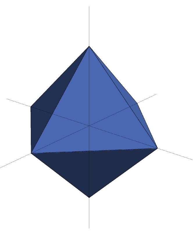
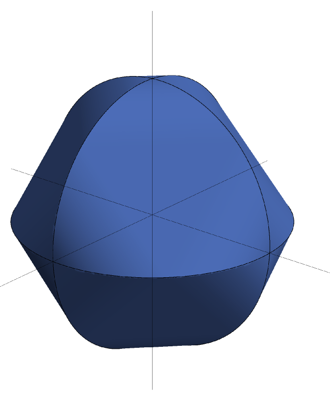
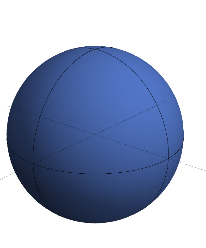
Figure 1: Unit balls of the $k$-support norm for $k\in\{1,2,3\}$.

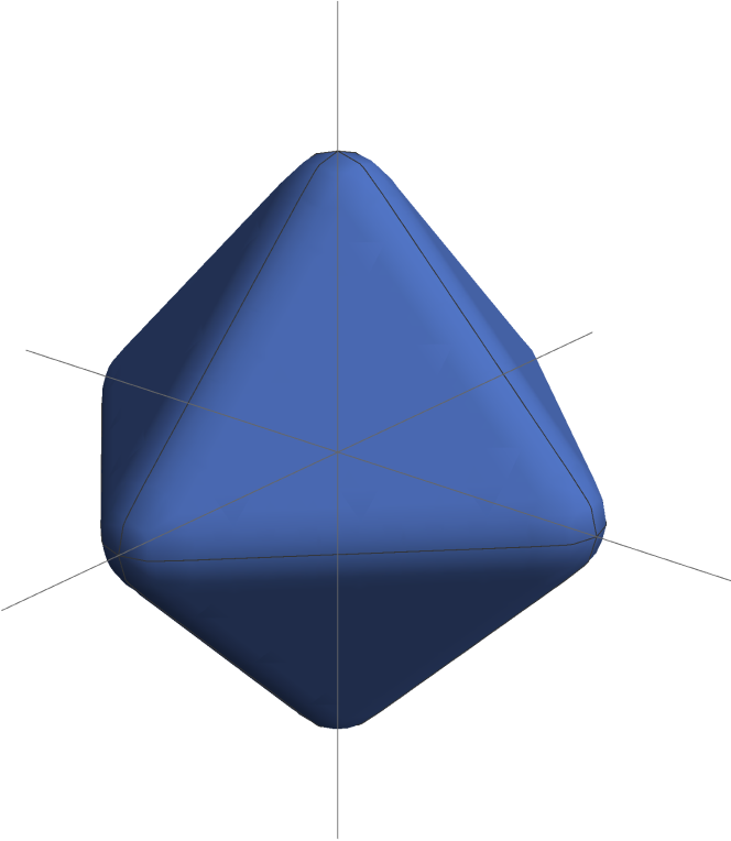
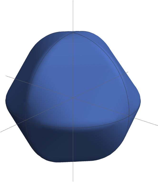
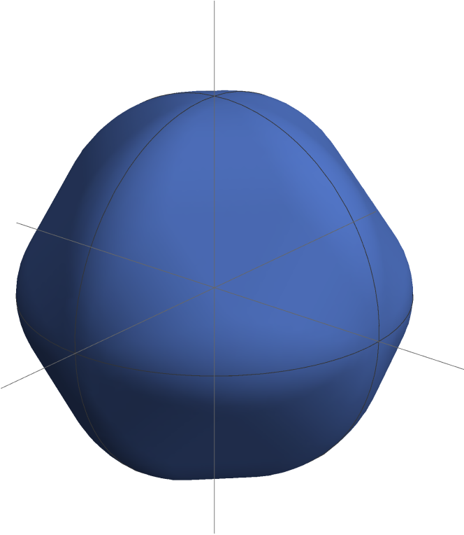
Figure 2: Unit balls of the box-norm, $(k,a)\in\{(1,0.15),(2,0.15),(2,0.40)\}$.

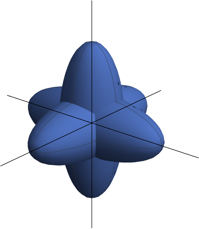
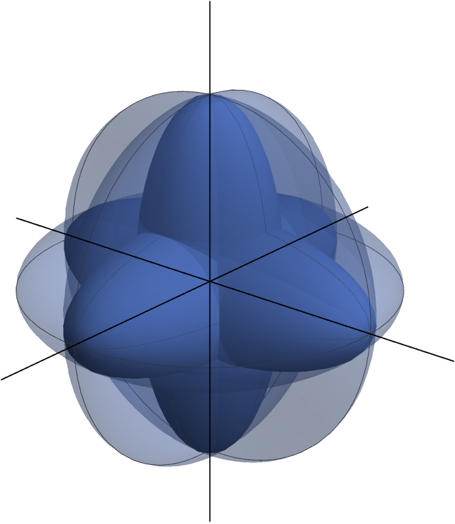
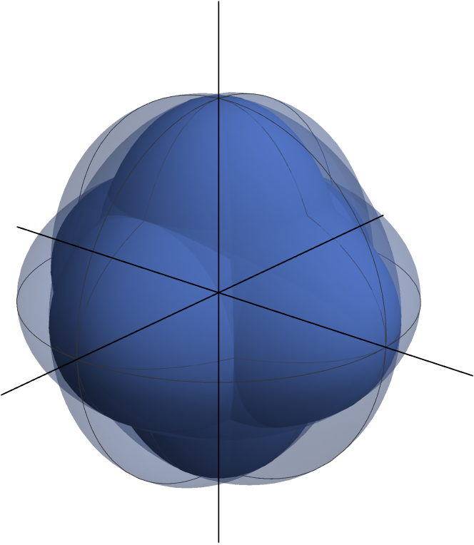
Figure 3: Primal box-norm component ellipsoids, $(k,a)\in\{(1,0.15),(2,0.15),(2,0.40)\}$.

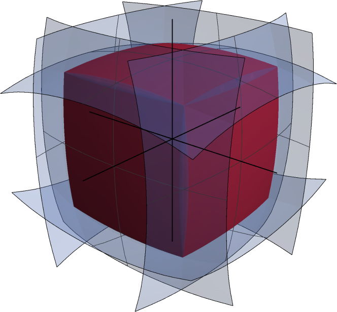
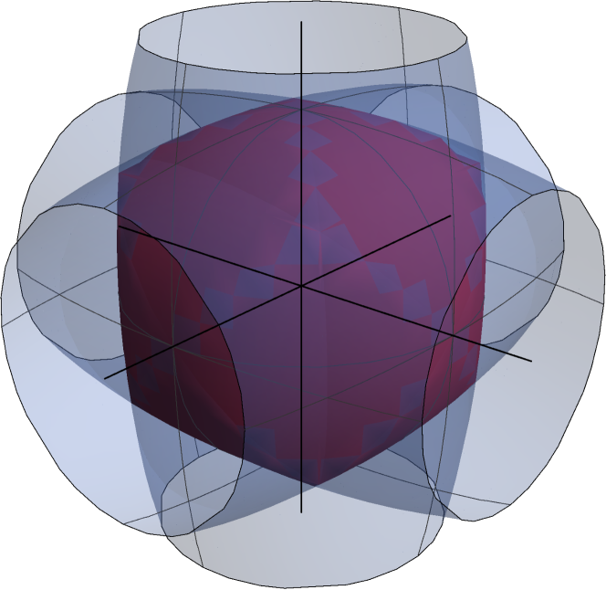
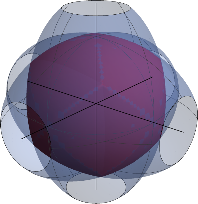
Figure 4: Dual box-norm unit balls and ellipsoids, $(k,a)\in\{(1,0.15),(2,0.15),(2,0.40)\}$. For $k=2$, only 3 tightest ellipsoids are shown.

4 Computation of the Norm and the Proximity Operator

In this section, we compute the norm and the proximity operator of the squared box-norm by explicitly solving the optimization problem (1). We also specialize our results to the $k$-support norm and comment on the improvement with respect the method by Argyriou et al. (2012). Recall that, for every vector $w\in{\mathbb{R}}^{d}$, $|w|^{\downarrow}$ denotes the vector obtained from $w$ by reordering its components so that they are non-increasing in absolute value.

Theorem 11

For every $w\in\mathbb{R}^{d}$ it holds that

$$\|w\|_{\rm box}^{2} =\frac{1}{b}\|w_{Q}\|_{2}^{2}+\frac{1}{p}\|w_{I}\|_{1}^{2}+\frac{1}{a}\|w_{L}\|_{2}^{2},$$ (22)

where $w_{Q}=(|w|^{\downarrow}_{1},\ldots,|w|^{\downarrow}_{q})$, $w_{I}=(|w|^{\downarrow}_{q+1},\ldots,|w|^{\downarrow}_{d-\ell})$, $w_{L}=(|w|^{\downarrow}_{d-\ell+1},\ldots,|w|^{\downarrow}_{d})$, $q$ and $\ell$ are the unique integers in $\{0,\ldots,d\}$ that satisfy $q+\ell\leq d$,

$$\frac{|w_{q}|}{b}\geq\frac{1}{p}\sum_{i=q+1}^{d-\ell}|w_{i}|>\frac{|w_{q+1}|}{b},\quad~{}~{}~{}\frac{|w_{d-\ell}|}{a}\geq\frac{1}{p}\sum_{i=q+1}^{d-\ell}|w_{i}|>\frac{|w_{d-\ell+1}|}{a},$$ (23)

$p=c-qb-\ell a$ and we have defined $|w_{0}|=\infty$ and $|w_{d+1}|=0$. Furthermore, the minimizer $\theta$ has the form

$$\theta_{i}=\begin{cases}b,\quad&\text{if }i\in\{1,\dots,q\},\\ p\frac{|w_{i}|}{\sum_{j=q+1}^{d-\ell}|w_{j}|},\quad&\text{if }i\in\{q+1,\dots,d-\ell\},\\ a,\quad&\text{otherwise}.\end{cases}$$

Proof  We solve the constrained optimization problem

$$\operatorname*{\vphantom{p}inf}\bigg{\{}\sum_{i=1}^{d}\frac{w_{i}^{2}}{\theta_{i}}:a\leq\theta_{i}\leq b,\sum_{i=1}^{d}\theta_{i}\leq c\bigg{\}}.$$ (24)

To simplify the notation we assume without loss of generality that $w_{i}$ are positive and ordered nonincreasing, and note that the optimal $\theta_{i}$ are ordered non increasing. To see this, let $\theta^{*}=\operatorname*{\arg\!\min}_{\theta\in\Theta}\sum_{i=1}^{d}\frac{w_{i}^{2}}{\theta_{i}}$. Now suppose that $\theta^{*}_{i}<\theta_{j}^{*}$ for some $i<j$ and define $\hat{\theta}$ to be identical to $\theta^{*}$, except with the $i$ and $j$ elements exchanged. The difference in objective values is

$$\sum_{i=1}^{d}\frac{w_{i}^{2}}{{\hat{\theta}}_{i}}-\sum_{i=1}^{d}\frac{w_{i}^{2}}{{\theta_{i}^{*}}}=(w_{i}^{2}-w_{j}^{2})\left(\frac{1}{\theta_{j}^{*}}-\frac{1}{\theta_{i}^{*}}\right),$$

which is negative so $\theta^{*}$ cannot be a minimizer.

We further assume without loss of generality that $w_{i}\neq 0$ for all $i$, and $c\leq db$ (see Remark 12 below). The objective is continuous and we take the infimum over a closed bounded set, so a solution exists and it is unique by strict convexity. Furthermore, since $c\leq db$, the sum constraint will be tight at the optimum. Consider the Lagrangian function

$$L(\theta,\alpha)=\sum_{i=1}^{d}\frac{w_{i}^{2}}{\theta_{i}}+\frac{1}{\alpha^{2}}\left(\sum_{i=1}^{d}\theta_{i}-c\right),$$ (25)

where $1/\alpha^{2}$ is a strictly positive multiplier, and $\alpha$ is to be chosen to make the sum constraint tight, call this value $\alpha^{*}$. Let $\theta^{*}$ be the minimizer of $L(\theta,\alpha^{*})$ over $\theta$ subject to $a\leq\theta_{i}\leq b$.

We claim that $\theta^{*}$ solves equation (24). Indeed, for any $\theta\in[a,b]^{d}$, $L(\theta^{*},\alpha^{*})\leq L(\theta,\alpha^{*})$, which implies that

$$\sum_{i=1}^{d}\frac{w_{i}^{2}}{\theta^{*}_{i}}\leq\sum_{i=1}^{d}\frac{w_{i}^{2}}{\theta_{i}}+\frac{1}{(\alpha^{*})^{2}}\left(\sum_{i=1}^{d}\theta_{i}-c\right).$$

If in addition we impose the constraint $\sum_{i=1}^{d}\theta_{i}\leq c$, the second term on the right hand side is at most zero, so we have for all such $\theta$ that

$$\sum_{i=1}^{d}\frac{w_{i}^{2}}{\theta^{*}_{i}}\leq\sum_{i=1}^{d}\frac{w_{i}^{2}}{\theta_{i}},$$

whence it follows that $\theta^{*}$ is the minimizer of (24).

We can therefore solve the original problem by minimizing the Lagrangian (25) over the box constraint. Due to the coupling effect of the multiplier, the problem is separable, and we can solve the simplified problem componentwise (see Micchelli et al., 2013, Theorem 3.1). For completeness we repeat the argument here. For every $w_{i}\in{\mathbb{R}}$ and $\alpha>0$, the unique solution to the problem $\min\{\frac{w_{i}^{2}}{\theta}+\frac{\theta}{\alpha^{2}}:a\leq\theta\leq b\}$ is given by

$$\theta=\begin{cases}b,\quad&\text{if }\alpha|w_{i}|>b,\\ \alpha|w|,&\text{if }b\geq\alpha|w_{i}|\geq a,\\ a,\quad&\text{if }a>\alpha|w_{i}|.\end{cases}$$ (26)

Indeed, for fixed $w_{i}$, the objective function is strictly convex on $\mathbb{R}^{d}_{++}$ and has a unique minimum on $(0,\infty)$ (see Figure 1.b in Micchelli et al. (2013) for an illustration). The derivative of the objective function is zero for $\theta=\theta^{*}:=\alpha|w_{i}|$, strictly positive below $\theta^{*}$ and strictly increasing above $\theta^{*}$. Considering these three cases the result follows and $\theta$ is determined by (26) where $\alpha$ satisfies $\sum_{i=1}^{d}\theta_{i}(\alpha)=c$.

The minimizer then has the form

$$\theta=(\underbrace{b,\ldots,b}_{q},\theta_{q+1},\ldots,\theta_{d-\ell},\underbrace{a,\ldots,a}_{\ell}),$$

where $q,\ell\in\{0,\ldots,d\}$ are determined by the value of $\alpha$ which satisfies

$$S(\alpha)=\sum_{i=1}^{d}\theta_{i}(\alpha)=qb+\sum_{i=q+1}^{d-\ell}\alpha|w_{i}|+\ell a=c,$$

i.e. $\alpha=p/\left(\sum_{i=q+1}^{d-\ell}|w_{i}|\right)$, where $p=c-qb-\ell a$.

The value of the norm follows by substituting $\theta$ into the objective and we get

$$\|w\|_{{\rm box}}^{2} =\sum_{i=1}^{q}\frac{|w_{i}|^{2}}{b}+\frac{1}{p}\Big{(}\sum_{i=q+1}^{d-\ell}|w_{i}|\Big{)}^{2}+\sum_{i=d-\ell+1}^{d}\frac{|w_{i}|^{2}}{a}=\frac{1}{b}\|w_{Q}\|_{2}^{2}+\frac{1}{p}\|w_{I}\|_{1}^{2}+\frac{1}{a}\|w_{L}\|_{2}^{2},$$

as required. We can further characterize $q$ and $\ell$ by considering the form of $\theta$. By construction we have $\theta_{q}\geq b>\theta_{q+1}$ and $\theta_{d-\ell}>a\geq\theta_{d-\ell+1}$, or equivalently

$$\frac{|w_{q}|}{b} \geq\frac{1}{p}\sum_{i=q+1}^{d-\ell}|w_{i}|>\frac{|w_{q+1}|}{b}~{}~{}~{}\textrm{and}~{}~{}~{}\frac{|w_{d-\ell}|}{a}\geq\frac{1}{p}\sum_{i=q+1}^{d-\ell}|w_{i}|>\frac{|w_{d-\ell+1}|}{a}.$$

The proof is completed.  

Remark 12

The case where some $w_{i}$ are zero follows from the case that we have considered in the theorem. If $w_{i}=0$ for $n<i\leq d$, then clearly we must have $\theta_{i}=a$ for all such $i$. We then consider the $n$-dimensional problem of finding $(\theta_{1},\ldots,\theta_{n})$ that minimizes $\sum_{i=1}^{n}\frac{w_{i}^{2}}{\theta_{i}}$, subject to $a\leq\theta_{i}\leq b$, and $\sum_{i=1}^{n}\theta_{i}\leq c^{\prime}$, where $c^{\prime}=c-(d-n)a$. As $c\geq da$ by assumption, we also have $c^{\prime}\geq na$, so a solution exists to the $n$-dimensional problem. If $c^{\prime}\geq bn$, then a solution is trivially given by $\theta_{i}=b$ for all $i=1,\dots,n$. In general, $c^{\prime}<bn$, and we proceed as per the proof of the theorem. Finally, a vector that solves the original $d$-dimensional problem will be given by $(\theta_{1},\ldots,\theta_{n},a,\ldots,a)$.

Theorem 11 suggests two methods for computing the box-norm. First, we can find $\alpha$ such that $S(\alpha)=c$; this value uniquely determines $\theta$ in (26), and the norm follows by substitution into the objective in (25). Alternatively, we identify $q$ and $\ell$ that jointly satisfy (23) and we compute the norm using (22). Taking advantage of the structure of $\theta$ in the former method leads to a computation time that is $\mathcal{O}(d\log d)$.

Theorem 13

The computation of the box-norm can be completed in $\mathcal{O}(d\log d)$ time.

Proof  Following Theorem 11, we need to determine $\alpha^{*}$ to satisfy the coupling constraint $S(\alpha^{*})=c$. Each component $\theta_{i}$ is a piecewise linear function in the form of a step function with a constant positive slope between the values $a/|w_{i}|$ and $b/|w_{i}|$. Let $\left\{\alpha^{i}\right\}_{i=1}^{2d}$ be the set of the $2d$ critical points, where the $\alpha^{i}$ are ordered nondecreasing. The function $S(\alpha)$ is a nondecreasing piecewise linear function with at most $2d$ critical points. We can find $\alpha^{*}$ by first sorting the points $\{\alpha^{i}\}$, finding $\alpha^{i}$ and $\alpha^{i+1}$ such that

$$S(\alpha^{i})\leq c\leq S(\alpha^{i+1})$$

by binary search, and then interpolating $\alpha^{*}$ between the two points. Sorting takes $\mathcal{O}(d\,\log d)$. Computing $S(\alpha^{i})$ at each step of the binary search is $\mathcal{O}(d)$, so $\mathcal{O}(d\,\log d)$ overall. Given $\alpha^{i}$ and $\alpha^{i+1}$, interpolating $\alpha^{*}$ is $\mathcal{O}(1)$, so the overall algorithm is $\mathcal{O}(d\,\log d)$ as claimed.  

The $k$-support norm is a special case of the box-norm, and as a direct corollary of Theorem 11 and Theorem 13, we recover (Argyriou et al., 2012, Proposition 2.1).

Corollary 14

For $w\in\mathbb{R}^{d}$, and $k\leq d$,

$$\|w\|_{(k)} =\Bigg{(}\sum_{j=1}^{q}(|w|^{\downarrow}_{j})^{2}+\frac{1}{k-q}\Big{(}\sum_{j=q+1}^{d}|w^{\downarrow}_{j}|\Big{)}^{2}\Bigg{)}^{\frac{1}{2}},$$

where $q$ is the unique integer in $\{0,k-1\}$ satisfying

$$|w_{q}|\geq\frac{1}{k-q}\sum_{j=q+1}^{d}|w_{j}|>|w_{q+1}|,$$ (27)

and we have defined $w_{0}=\infty$. Furthermore, the norm can be computed in $\mathcal{O}(d\log d)$ time.

4.1 Proximity Operator

Proximal gradient methods can be used to solve optimization problems of the form

$$\min_{w}f(w)+\lambda g(w),~{}~{}~{}w\in{\mathbb{R}}^{d},$$

where $f$ is a convex loss function with Lipschitz continuous gradient, $\lambda>0$ is a regularization parameter, and $g$ is a convex function for which the proximity operator can be computed efficiently, see Nesterov (2007); Combettes and Pesquet (2011); Beck and Teboulle (2009) and references therein. The proximity operator of $g$ with parameter $\rho>0$ is defined as

$$\operatorname{prox}_{\rho g}(w)=\operatorname*{\arg\!\min}\left\{\frac{1}{2}\|x-w\|^{2}+\rho g(x):x\in{\mathbb{R}}^{d}\right\}.$$

We now use the infimum formulation of the box-norm to derive the proximity operator of the squared norm.

Theorem 15

The proximity operator of the square of the box-norm at point $w\in\mathbb{R}^{d}$ with parameter $\frac{\lambda}{2}$ is given by $\operatorname{prox}_{\frac{\lambda}{2}\|\cdot\|_{{\rm box}}^{2}}(w)=(\frac{\theta_{1}w_{1}}{\theta_{1}+\lambda},\dots,\frac{\theta_{d}w_{d}}{\theta_{d}+\lambda})$, where

$$\theta_{i} =\begin{cases}b,&\text{if }\,\alpha|w_{i}|-\lambda>b,\\ \alpha|w_{i}|-\lambda,&\text{if }\,b\geq\alpha{|w_{i}|}-\lambda\geq a,\\ a,&\text{if }\,a>\alpha|w_{i}|-\lambda,\end{cases}$$

and $\alpha$ is chosen such that $S(\alpha):=\sum_{i=1}^{d}\theta_{i}(\alpha)=c$. Furthermore, the computation of the proximity operator can be completed in $\mathcal{O}(d\log d)$ time.

Proof  Using the infimum formulation of the norm, we solve

$$\min_{x\in\mathbb{R}^{d}}\operatorname*{\vphantom{p}inf}_{\theta\in\Theta}\,\left\{\frac{1}{2}\sum_{i=1}^{d}(x_{i}-w_{i})^{2}+\frac{\lambda}{2}\sum_{i=1}^{d}\frac{x_{i}^{2}}{\theta_{i}}\right\}.$$

We can exchange the order of the optimization and solve for $x$ first. The problem is separable and a direct computation yields that $x_{i}=\frac{\theta_{i}w_{i}}{\theta_{i}+\lambda}$. Discarding a multiplicative factor of $\lambda/2$, and noting that the infimum is attained, the problem in $\theta$ becomes

$$\min_{\theta}\bigg{\{}\sum_{i=1}^{d}\frac{w_{i}^{2}}{\theta_{i}+\lambda}:{a\leq\theta_{i}\leq b,\sum_{i=1}^{d}\theta_{i}\leq c}\,\bigg{\}}.$$

Note that this is the same as computing a box-norm in accordance with Proposition 8. Specifically, this is exactly like problem (24) after the change of variable $\theta^{\prime}_{i}=\theta_{i}+\lambda$. The remaining part of the proof then follows in a similar manner to the proof of Theorem 11.  

Algorithm 1 illustrates the computation of the proximity operator for the squared box-norm in $\mathcal{O}(d\log d)$ time. This includes the $k$-support as a special case, where we let $a$ tend to zero, and set $b=1$ and $c=k$, which improves upon the complexity of the $\mathcal{O}(d(k+\log d))$ computation provided in Argyriou et al. (2012), and we illustrate the improvement empirically in Table 1. We summarize this in the following corollary.

Corollary 16

The proximity operator of the square of the $k$-support norm at point $w$ with parameter $\frac{\lambda}{2}$ is given by $\operatorname{prox}_{\frac{\lambda}{2}\|\cdot\|_{\Theta}^{2}}(w)=x$, where $x_{i}=\frac{\theta_{i}w_{i}}{\theta_{i}+\lambda}$, and

$$\theta_{i} =\begin{cases}1,&\text{if }\,\alpha|w_{i}|>\lambda+1,\\ \alpha|w_{i}|-\lambda,&\text{if }\,\lambda+1\geq\alpha|w_{i}|\geq\lambda\\ 0,&\text{if }\,\lambda>\alpha|w_{i}|,\end{cases}$$

where $\alpha$ is chosen such that $S(\alpha)=k$. Furthermore, the proximity operator can be computed in $\mathcal{O}(d\log d)$ time.

Algorithm 1 Computation of $x=\operatorname{prox}_{\frac{\lambda}{2}\|\cdot\|_{\rm box}^{2}}\left(w\right)$.

0:  parameters $a$, $b$, $c$, $\lambda$.

  1. Sort points $\left\{\alpha^{i}\right\}_{i=1}^{2d}=\left\{\frac{a+\lambda}{|w_{j}|},\frac{b+\lambda}{|w_{j}|}\right\}_{j=1}^{d}$ such that $\alpha^{i}\leq\alpha^{i+1}$;

  2. Identify points $\alpha^{i}$ and $\alpha^{i+1}$ such that $S(\alpha^{i})\leq c$ and $S(\alpha^{i+1})\geq c$ by binary search;

  3. Find $\alpha^{*}$ between $\alpha^{i}$ and $\alpha^{i+1}$ such that $S(\alpha^{*})=c$ by linear interpolation;

  4. Compute $\theta_{i}(\alpha^{*})$ for $i=1\ldots,d$;

  5. Return $x_{i}=\frac{\theta_{i}w_{i}}{\theta_{i}+\lambda}$ for $i=1\ldots,d$.

5 Spectral Norms

We now turn our focus to the matrix norms. For this purpose, we recall that a norm $\|\cdot\|$ on $\mathbb{R}^{d\times T}$ is called orthogonally invariant if $\|W\|=\|UWV\|$, for any orthogonal matrices $U\in\mathbb{R}^{d\times d}$ and $V\in\mathbb{R}^{T\times T}$. A classical result by Von Neumann (1937) establishes that a norm is orthogonally invariant if and only if it is of the form $\|W\|=g(\sigma(W))$, where $\sigma(W)$ is the vector formed by the singular values of $W$ in nonincreasing order, and $g$ is a symmetric gauge function, that is a norm which is invariant under permutations and sign changes of the vector components.

Lemma 17

If $\Theta$ is a convex bounded subset of the strictly positive orthant in $\mathbb{R}^{d}$ which is invariant under permutations, then $\|\cdot\|_{\Theta}$ is a symmetric gauge function.

Proof  Let $g(w)=\|w\|_{\Theta}$. We need to show that $g$ is a norm which is invariant under permutations and sign changes. By Proposition 2, $g$ is a norm, so it remains to show that $g(w)=g(Pw)$ for every permutation matrix $P$, and $g(Jw)=g(w)$ for every diagonal matrix $J$ with entries $\pm 1$. The former property follows since the set $\Theta$ is permutation invariant. The latter property is true because the objective function in (1) involves the squares of the components of $w$.  

In particular, this readily applies to both the $k$-support norm and the box-norm. We can therefore extend both norms to orthogonally invariant norms, which we term the spectral $k$-support norm and the spectral box-norm respectively, and which we write (with some abuse of notation) as $\|W\|_{(k)}=\|\sigma(W)\|_{(k)}$ and $\|W\|_{\rm box}=\|\sigma(W)\|_{\rm box}$. We note that since the $k$-support norm subsumes the $\ell_{1}$ and $\ell_{2}$-norms for $k=1$ and $k=d$ respectively, the corresponding spectral $k$-support norms are equal to the trace and Frobenius norms respectively.

A number of properties of the vector norms translate in the natural manner to the matrix norms. We first characterize the unit ball of the spectral $k$-support norm.

Proposition 18

The unit ball of the spectral $k$-support norm is the convex hull of the set of matrices of rank at most k and Frobenius norm no greater than one.

Proof  For any $W\in\mathbb{R}^{d\times T}$, define the following sets

$$T_{k} =\{W\in\mathbb{R}^{d\times T}:\textrm{rank}(W)\leq k,~{}\|W\|_{F}\leq 1\},\quad A_{k}=\textrm{co}(T_{k}),$$

and consider the following functional

$$\lambda(W) =\operatorname*{\vphantom{p}inf}\{\lambda>0:W\in\lambda A_{k}\},~{}~{}~{}W\in\mathbb{R}^{d\times T}.$$ (28)

We will apply Lemma 23 in the appendix to the set $A_{k}$. To do this, we need to show that the set $A_{k}$ is bounded, convex, symmetric and absorbing. The first three are clearly satisfied. To see that it is absorbing, let $W\in\mathbb{R}^{d\times T}$ have singular value decomposition $U\Sigma V^{\scriptscriptstyle\top}$, and let $r=\min(d,T)$. If $W$ is zero then clearly $W\in A_{k}$, so assume it is non zero.

For $i\in{\mathbb{N}}_{r}$ let $S_{i}\in{\mathbb{R}}^{d\times T}$ have entry $(i,i)$ equal to $1$, and all remaining entries zero. We then have

$$W =U\Sigma V^{\scriptscriptstyle\top}=U\left(\sum_{i=1}^{r}\sigma_{i}S_{i}\right)V^{\scriptscriptstyle\top}=\left(\sum_{i=1}^{d}\sigma_{i}\right)\sum_{i=1}^{r}\frac{\sigma_{i}}{\sum_{j=1}^{r}\sigma_{j}}(US_{i}V^{\scriptscriptstyle\top})=:\lambda\sum_{i=1}^{r}\beta_{i}Z_{i}.$$

Now for each $i$, $\|Z_{i}\|_{F}=\|S_{i}\|_{F}=1$, and $\textrm{rank}(Z_{i})=\textrm{rank}(S_{i})=1$, so $Z_{i}\in T_{k}$ for any $k\geq 1$. Furthermore $\beta_{i}\in[0,1]$ and $\sum_{i=1}^{r}\beta_{i}=1$, that is $(\beta_{1},\ldots,\beta_{r})\in\Delta^{r-1}$, so $\frac{1}{\lambda}W$ is a convex combination of $Z_{i}$, in other words $W\in\lambda A_{k}$, and we have shown that $A_{k}$ is absorbing. It follows that $A_{k}$ satisfies the hypotheses of Lemma 23, where we let $C=A_{k}$, hence $\lambda$ defines a norm on ${\mathbb{R}}^{d\times T}$ with unit ball equal to $A_{k}$.

Since the constraints in $T_{k}$ involve spectral functions, the sets $T_{k}$ and $A_{k}$ are invariant to left and right multiplication by orthogonal matrices. It follows that $\lambda$ is a spectral function, that is $\lambda(W)$ is defined in terms of the singular values of $W$. By von Neumann’s Theorem (Von Neumann, 1937) the norm it defines is orthogonally invariant and we have

$$\lambda(W) =\operatorname*{\vphantom{p}inf}\{\lambda>0:W\in\lambda A_{k}\}=\operatorname*{\vphantom{p}inf}\{\lambda>0:\sigma(W)\in\lambda C_{k}\}=\|\sigma(W)\|_{(k)}$$

where we have used Corollary 24, which states that $C_{k}$ is the unit ball of the $k$-support norm. It follows that the norm defined by (28) is the spectral $k$-support norm with unit ball given by $A_{k}$.  

Referring to the unit ball characterization of the $k$-support norm, we note that the restriction on the cardinality of the vectors which define the extreme points of the unit ball naturally extends to a restriction on the rank operator in the matrix setting. Furthermore, as noted by Argyriou et al. (2012), regularization using the $k$-support norm encourages vectors to be sparse, but less so than the $\ell_{1}$-norm. In matrix regularization problems, Proposition 18 suggests that the spectral $k$-support norm for $k>1$ encourages matrices to have low rank, but less so than the trace norm. This is intuitive as the extreme points of the unit ball have rank at most $k$.

As in the case of the vector norm (Proposition 8), the spectral box-norm (or cluster norm – see below) can be written as a perturbation of the spectral $k$-support norm with a quadratic term.

Proposition 19

Let $\|\cdot\|_{{\rm box}}$ be a matrix box-norm with parameters $a,b,c$ and let $k=\frac{c-da}{b-a}$. Then

$$\|W\|_{{\rm box}}^{2} =\min_{Z\in{\mathbb{R}}^{d\times T}}\left\{\frac{1}{a}\|W-Z\|_{F}^{2}+\frac{1}{b-a}\|Z\|_{(k)}^{2}\right\}.$$

Proof  By von Neumann’s trace inequality (Theorem 25 in the appendix) we have

$$\frac{1}{a}\|W-Z\|_{F}^{2}+\frac{1}{b-a}\|Z\|_{(k)}^{2} =\frac{1}{a}\left(\|W\|_{F}^{2}+\|Z\|_{F}^{2}-2\langle W,Z\rangle\right)+\frac{1}{b-a}\|Z\|_{(k)}^{2}$$

$$\geq\frac{1}{a}\left(\|\sigma(W)\|_{2}^{2}+\|\sigma(Z)\|_{2}^{2}-2\langle\sigma(W),\sigma(Z)\rangle\right)+\frac{1}{b-a}\|\sigma(Z)\|_{(k)}^{2}$$

$$=\frac{1}{a}\|\sigma(W)-\sigma(Z)\|_{2}^{2}+\frac{1}{b-a}\|\sigma(Z)\|_{(k)}^{2}.$$

Furthermore the inequality is tight if $W$ and $Z$ have the same ordered set of singular vectors. Hence

$$\min_{Z\in{\mathbb{R}}^{d\times T}}\left\{\frac{1}{a}\|W-Z\|_{F}^{2}+\frac{1}{b-a}\|Z\|_{(k)}^{2}\right\} =\min_{z\in{\mathbb{R}}^{d}}\left\{\frac{1}{a}\|\sigma(W)-z\|_{2}^{2}+\frac{1}{b-a}\|z\|_{(k)}^{2}\right\}=\|\sigma(W)\|_{{\rm box}}^{2},$$

where the last equality follows by Proposition 8.  

In other words, this result shows that the (scaled) squared spectral box-norm can be seen as the Moreau envelope of a squared spectral $k$-support norm.

5.1 Proximity Operator for Orthogonally Invariant Norms

The computational considerations outlined in Section 4 can be naturally extended to the matrix setting by using von Neumann’s trace inequality stated in the appendix. Here we comment on the computation of the proximity operator, which is important for our numerical experiments in Section 7. The proximity operator of an orthogonally invariant norm $\|\cdot\|=g(\sigma(\cdot))$ is given by

$$\operatorname{prox}_{\|\cdot\|}(W)=U\text{diag}(\operatorname{prox}_{g}(\sigma(W)))V^{\scriptscriptstyle\top},~{}~{}~{}W\in\mathbb{R}^{m\times T},$$

where $U$ and $V$ are the matrices formed by the left and right singular vectors of $W$ (see e.g. Argyriou et al., 2011, Prop. 3.1). Using this result we can employ proximal gradient methods to solve matrix regularization problems using the square of the spectral $k$-support and box-norms.

6 Multitask Learning

In this section, we address multitask learning, a framework in which spectral regularizers have successfully been used to learn a set of regression or binary classification tasks. Within this setting each column of the matrix $W$ represents one of the task weight vectors. By leveraging the commonalities between the tasks, learning can often be improved compared to solving each task in isolation (see e.g. Evgeniou et al., 2005; Argyriou et al., 2007, 2008; Jacob et al., 2009a; Cavallanti et al., 2010, and references therein). A natural assumption that arises in applications is that the tasks are clustered. The cluster norm was introduced by Jacob et al. (2009a) as a means to favour this structure. We show that this norm is equivalent to the spectral box-norm and then address the issue of centering the norm.

6.1 Clustering the Tasks

A general approach to multitask learning is based on the regularization problem

$$\min_{W\in\mathbb{R}^{d\times T}}{\cal L}(W)+\lambda\Omega(W)$$

where $W=[w_{1},\ldots,w_{T}]$ is the $d\times T$ matrix whose columns represent the task vectors, $\Omega$ is a regularizer which incorporates prior knowledge of sharing between tasks and ${\cal L}$ is the compound empirical error. That is, ${\cal L}(W)=\frac{1}{Tn}\sum_{t=1}^{T}\sum_{i=1}^{n}\ell(y_{i}^{t},{\langle}w_{t},x_{i}^{t}{\rangle})$ where $(x_{1}^{t},y_{1}^{t}),\dots,(x_{n}^{t},y_{n}^{t})\in\mathbb{R}^{d}\times\mathbb{R}$ are the training points for task $t$ (for simplicity we assume that each task has the same number $n$ of training points) and $\ell$ is a convex loss function.

Jacob et al. (2009a) consider a composite penalty which encourages the tasks to be clustered into $Q<T$ groups. To introduce their setting we require some more notation. Let $\mathcal{J}_{q}\subseteq{{\mathbb{N}}}_{T}$ be the set of tasks in cluster $q\in{{\mathbb{N}}}_{Q}$ and let $T_{q}=|\mathcal{J}_{q}|\geq 0$ be the number of tasks in cluster $q$, so that $\sum_{q=1}^{Q}T_{q}=T$. The clustering uniquely defines the $T\times T$ normalized connectivity matrix $M$ where $M_{st}=\frac{1}{T_{q}}$ if $s,t\in{\cal J}_{q}$ and $M_{st}=0$ otherwise. We let $\bar{w}=\frac{1}{T}\sum_{t=1}^{T}w_{t}$ be the mean weight vector, $\bar{w}_{q}=\frac{1}{T_{q}}\sum_{t\in\mathcal{J}_{q}}w_{t}$ be the mean weight vector of tasks in cluster $q$ and define the $T\times T$ orthogonal projection matrices $U=11^{\scriptscriptstyle\top}/T$ and $\Pi=I-U$. Note that $W\Pi=[w_{1}-{\bar{w}},\dots,w_{T}-{\bar{w}}]$. Finally, let $r=\min(d,T)$.

Using this notation, we introduce the three seminorms

$$\Omega_{\rm m}(W) =T\|\bar{w}\|^{2}={\rm tr}\left(WUW^{\scriptscriptstyle\top}\right)$$

$$\Omega_{\rm b}(W) =\sum_{q=1}^{Q}T_{q}\|\bar{w}_{q}-\bar{w}\|^{2}={\rm tr}\left(W(M-U)W^{\scriptscriptstyle\top}\right)$$

$$\Omega_{\rm w}(W) =\sum_{q=1}^{Q}\sum_{t\in\mathcal{J}_{q}}\|w_{t}-\bar{w}_{q}\|^{2}={\rm tr}\left(W(I-M)W^{\scriptscriptstyle\top}\right),$$

each of which captures a different aspect of the clustering: $\Omega_{\rm m}$ penalizes the total mean of the weight vectors, $\Omega_{\rm b}$ measures how close to each other the clusters are (between cluster variance), and $\Omega_{\rm w}$ measures the compactness of the clusters (within cluster variance). Scaling the three penalties by positive parameters $\epsilon_{\rm m}$, $\epsilon_{\rm b}$ and $\epsilon_{\rm w}$ respectively, we obtain the composite penalty $\epsilon_{\rm m}\Omega_{\rm m}+\epsilon_{\rm b}\Omega_{\rm b}+\epsilon_{\rm w}\Omega_{\rm w}$. The first term $\Omega_{\rm m}$ does not depend on the connectivity matrix $M$, and it can be included in the error term. The remaining two terms depend on $M$, which in general may not be known a-priori. Jacob et al. (2009a) propose to learn the clustering by minimizing with respect to matrix $M$, under the assumption that $\epsilon_{\rm w}\geq\epsilon_{\rm b}$; this assumption is reasonable as we care more about enforcing a small variance of parameters within the clusters than between them. Using the elementary properties that $M-U=M\Pi=\Pi M\Pi$ and $I-M=(I-M)\Pi=\Pi(I-M)\Pi$ and letting $\widetilde{M}=M\Pi$, we rewrite

$$\epsilon_{\rm b}\Omega_{\rm b}(W)+\epsilon_{\rm w}\Omega_{\rm w}(W)={\rm tr}\left({W}\Pi\big{(}\epsilon_{\rm b}\widetilde{M}+\epsilon_{\rm w}(I-\widetilde{M})\big{)}\Pi{W}^{\scriptscriptstyle\top}\right)={\rm tr}\left({W}\Pi{\Sigma}^{-1}\Pi{W}^{\scriptscriptstyle\top}\right)$$ (29)

where we have defined $\Sigma^{-1}=\epsilon_{\rm b}\widetilde{M}+\epsilon_{\rm w}(I-\widetilde{M})$. Since $\widetilde{M}$ is an orthogonal projection, the matrix $\Sigma$ is well defined and we have

$$\Sigma=(\epsilon_{\rm b}^{-1}-\epsilon_{\rm w}^{-1}){\widetilde{M}}+\epsilon_{\rm w}^{-1}I.$$ (30)

The expression in the right hand side of equation (29) is jointly convex in $W$ and $\Sigma$ (see e.g. Boyd and Vandenberghe, 2004), however the set of matrices $\Sigma$ defined by equation (30), generated by letting ${\widetilde{M}}=M\Pi$ vary, is nonconvex, because $M$ takes values on a nonconvex set. To address this, Jacob et al. (2009a) relax the constraint on matrix ${\widetilde{M}}$ to the set $\{0\preceq{\widetilde{M}}\preceq I,~{}{\rm tr}{\widetilde{M}}\leq Q-1\}$. This in turn induces the convex constraint set for $\Sigma$

$${\cal S}_{Q,T}=\left\{\Sigma\in{\mathbb{R}}^{T\times T}:\Sigma=\Sigma^{\scriptscriptstyle\top},~{}\epsilon_{\rm w}^{-1}I\preceq\Sigma\preceq\epsilon_{\rm b}^{-1}I,~{}{\rm tr}\,\Sigma\leq(\epsilon_{\rm b}^{-1}-\epsilon_{\rm w}^{-1})(Q-1)+\epsilon_{\rm w}^{-1}T\right\}.$$

In summary Jacob et al. (2009a) arrive at the optimization problem

$$\min_{W\in\mathbb{R}^{d\times T}}{\bar{\cal L}}(W)+\lambda\|W\Pi\|_{\rm cl}^{2}$$ (31)

where ${\bar{\cal L}}(W)={\cal L}(W)+\lambda\epsilon_{\rm m}\,{\rm tr}(WUW^{\scriptscriptstyle\top})$ and $\|\cdot\|_{\rm cl}$ is the cluster norm defined by the equation

$$\|W\|_{\rm cl}=\sqrt{\operatorname*{\vphantom{p}inf}_{\Sigma\in{\cal S}_{Q,T}}{\rm tr}(\Sigma^{-1}W^{\scriptscriptstyle\top}W)}.$$ (32)

6.2 The Cluster Norm and the Spectral Box-Norm

We now discuss the cluster norm in the context of the spectral box-norm. Jacob et al. (2009a) state that the cluster norm of $W$ equals what we in this paper have termed the spectral box-norm, with parameters $a={\epsilon_{\rm w}}^{-1}$, $b=\epsilon_{\rm b}^{-1}$ and $c=(T-Q+1)\epsilon_{\rm w}^{-1}+(Q-1)\epsilon_{\rm b}^{-1}$. Here we prove this fact. Denote by $\lambda_{i}(\cdot)$ the eigenvalues of a matrix which we write in non increasing order $\lambda_{1}(\cdot)\geq\lambda_{2}(\cdot)\geq\ldots\geq\lambda_{d}(\cdot)$. Note that if $\theta_{i}$ are the eigenvalues of $\Sigma$ then $\theta_{i}=\lambda_{d-i+1}(\Sigma^{-1})$. We have that

$${\rm tr}(\Sigma^{-1}W^{\scriptscriptstyle\top}W)\geq\sum_{i=1}^{r}\lambda_{d-i+1}(\Sigma^{-1})\lambda_{i}(W^{\scriptscriptstyle\top}W)=\sum_{i=1}^{r}\frac{\sigma_{i}^{2}(W)}{\theta_{i}}$$

where the inequality follows by Lemma 26 (stated in the appendix) for $A=\Sigma^{-1}$ and $B=W^{\scriptscriptstyle\top}W\succeq 0$. Since this inequality is attained whenever $\Sigma=U{\rm diag}(\theta)U$, where $U$ are the eigenvectors of $W^{\scriptscriptstyle\top}W$, we see that the cluster norm coincides with the spectral box-norm, that is $\|W\|_{\rm cl}=\|\sigma(W)\|_{\Theta}$ for $\Theta=\{\theta\in[a,b]^{r}:\sum_{i=1}^{r}\theta_{i}\leq c\}$. In light of our observations in Section 5, we also see that the spectral $k$-support norm is a special case of the cluster norm, where we let $a$ tend to zero, $b=1$ and $c=k$, where $k=Q-1$. More importantly the cluster norm is a perturbation of the spectral $k$-support norm. Moreover, the methods to compute the norm and its proximity operator (cf. Theorems 11 and 15) can directly be applied to the cluster norm using von Neumann’s trace inequality (see Theorem 25 in the appendix).

6.3 Optimization with Centered Spectral $\Theta$-Norms

Centering a matrix has been shown to improve learning in other multitask learning problems, for example Evgeniou et al. (2005) reported improved results using the trace norm. It is therefore valuable to address the problem of how to solve a regularization problem of the type

$$\min_{W\in\mathbb{R}^{d\times T}}{\bar{\cal L}}(W)+\lambda\|W\Pi\|_{\Theta}^{2}$$ (33)

in which the regularizer is applied to the matrix $W\Pi=[w_{1}-{\bar{w}},\dots,w_{T}-{\bar{w}}]$. To this end, let $\Theta$ be a bounded and convex subset of $\mathbb{R}_{++}^{r}$ which is invariant under permutation. We have already noted that the function defined, for every $W\in{\mathbb{R}}^{d\times T}$, as

$$\|W\|_{\Theta}:=\|\sigma(W)\|_{\Theta},$$

is an orthogonally invariant norm. In particular, problem (33) includes regularization with the centered cluster norm outlined above.

Note that right multiplication by the centering operator $\Pi$, is invariant to a translation of the columns of the matrix by a fixed vector, that is, for every $z\in{\mathbb{R}}^{d}$, we have $[w_{1}+z,\dots,w_{T}+z]\Pi=W\Pi$. The quadratic term ${\epsilon_{\rm m}}{\rm tr}(WUW^{\scriptscriptstyle\top})$, which is included in the error, implements square norm regularization of the mean of the tasks, which can help to prevent overfitting. However, in the remainder of this section this term plays no role in the analysis, which equally applies to the case that $\epsilon_{\rm m}=0$.

In order to solve the problem (33) with a centered regularizer the following lemma is key.

Lemma 20

Let $r=\min(d,T)$ and let $\Theta$ be a bounded and convex subset of $\mathbb{R}_{++}^{r}$ which is invariant under permutation. For every $W=[w_{1},\dots,w_{T}]\in{\mathbb{R}}^{d\times T}$, it holds that

$$\|W\Pi\|_{\Theta}=\min_{z\in{\mathbb{R}}^{d}}\|[w_{1}-z,\ldots,w_{T}-z]\|_{\Theta}.$$

Proof  Given the set $\Theta$ we define the set $\Theta^{(T)}=\{\Sigma\in{\bf S}_{++}^{T},~{}\lambda(\Sigma)\in\Theta\}$ and $\Theta^{(d)}=\{D\in{\bf S}_{++}^{d}:\lambda(D)\in\Theta\}$. It follows from Lemma 26 that

$$\|W\|_{\Theta}^{2}\equiv\|\sigma(W)\|_{\Theta}^{2}=\operatorname*{\vphantom{p}inf}_{\Sigma\in\Theta^{(T)}}{\rm tr}\left(\Sigma^{-1}W^{\scriptscriptstyle\top}W\right)=\operatorname*{\vphantom{p}inf}_{D\in\Theta^{(d)}}{\rm tr}\left(D^{-1}WW^{\scriptscriptstyle\top}\right).$$

Using the second identity and recalling that $W\Pi=[w_{1}-\bar{w},\ldots,w_{T}-\bar{w}]$, we have that

$$\|W\Pi\|_{\Theta}^{2} =\operatorname*{\vphantom{p}inf}_{D\in\Theta^{(d)}}{\rm tr}((W\Pi)^{\scriptscriptstyle\top}D^{-1}(W\Pi))$$

$$=\operatorname*{\vphantom{p}inf}_{D\in\Theta^{(d)}}\sum_{t=1}^{T}(w_{t}-\bar{w})^{\scriptscriptstyle\top}D^{-1}(w_{t}-\bar{w})=\operatorname*{\vphantom{p}inf}_{D\in\Theta^{(d)}}\min_{z\in\mathbb{R}^{d}}\sum_{t=1}^{T}(w_{t}-z)^{\scriptscriptstyle\top}D^{-1}(w_{t}-z)$$

where in the last step we used the fact that the quadratic form $\sum_{t=1}^{T}(w_{t}-z)^{\scriptscriptstyle\top}D^{-1}(w_{t}-z)$ is minimized at $z=\bar{w}$. The result now follows by interchanging the infimum and the minimum in the last expression and using the definition of the $\Theta$-norm.  

Using this lemma, we rewrite problem (31) as

$$\min_{W\in\mathbb{R}^{d\times T}}\min_{z\in\mathbb{R}^{d}}{\bar{\cal L}}(W)+\lambda\|[w_{1}-z,\dots,w_{T}-z]\|_{\Theta}.$$

Letting ${v}_{t}=w_{t}-z$, and ${V}=[v_{1},\ldots,v_{T}]$, we obtain the equivalent problem

$$\min_{({V},z)\in\mathbb{R}^{d\times T}\times\mathbb{R}^{d}}{\bar{{\cal L}}}(V+z1^{\scriptscriptstyle\top})+\lambda\|{V}\|_{\Theta}^{2}.$$ (34)

This problem is of the form $f(V,z)+\lambda g(V,z)$, where $g(V,z)=\|V\|_{\Theta}$. Using this formulation, we can directly apply the proximal gradient method using the proximity operator computation for the vector norm, since $\operatorname{prox}_{g}(V_{0},z_{0})=(\operatorname{prox}_{\lambda\|\cdot\|_{\Theta}}(V_{0}),z_{0})$. This observation establishes that, whenever the proximity operator of the spectral $\Theta$-norm is available, we can use proximal gradient methods with minimal additional effort to perform optimization with the corresponding centered spectral $\Theta$-norm. For example, this is the case with the trace norm, the spectral $k$-support norm and the spectral box-norm or cluster norm.

7 Numerical Experiments

Argyriou et al. (2012) demonstrated the good estimation properties of the vector $k$-support norm compared to the Lasso and the elastic net. In this section, we investigate the matrix norms and report on their statistical performance in matrix completion and multitask learning experiments on simulated as well as benchmark real datasets. We also offer an interpretation of the role of the parameters in the box-norm and we empirically verify the improved performance of the proximity operator computation of Algorithm 1 (see Table 1).

We compare the spectral $k$-support norm (k-sup) and the spectral box-norm (box) to the baseline trace norm (trace) (see e.g. Argyriou et al., 2007; Mazumder et al., 2010; Srebro et al., 2005; Toh and Yun, 2011), matrix elastic net (el.net) (Li et al., 2012) and, in the case of multitask learning, the Frobenius norm (fr), which we recall is equivalent to the spectral $k$-support norm when $k=d$. As we highlighted in Section 6.3, centering a matrix can lead to improvements in learning. For datasets which we expect to exhibit clustering we therefore also apply centered versions of the norms, c-fr, c-trace, c-el.net, c-k-sup, c-box.

We report test error and standard deviation, matrix rank ($r$) and optimal parameter values for $k$ and $a$, which are determined by validation. We used a $t$-test to determine the statistical significance of the difference in performance between the regularizers, at a level of $p<0.001$.

To solve the optimization problem we used an accelerated proximal gradient method (FISTA), (see e.g. Beck and Teboulle, 2009; Nesterov, 2007), using the percentage change in the objective as convergence criterion, with a tolerance of $10^{-5}$ ($10^{-3}$ for real matrix completion experiments).

As is typical with spectral regularizers such as the trace norm, we found that the spectrum of the learned matrix exhibited a rapid decay to zero. In order to explicitly impose a low rank on the final matrix, we included a thresholding step at the end of the optimization. For the matrix completion experiments, the thresholding level was chosen by validation. Matlab code used in the experiments is available at http://www0.cs.ucl.ac.uk/staff/M.Pontil/software.html.

Table 1: Comparison of proximity operator algorithms for the $k$-support norm (time in seconds), $k=0.05d$. Algorithm 1 is our method, Algorithm 2 is the method in Argyriou et al. (2012).

$d$	1,000	2,000	4,000	8,000	16,000	32,000
Algorithm 1	0.0011	0.0016	0.0026	0.0046	0.0101	0.0181
Algorithm 2	0.0443	0.1567	0.5907	2.3065	9.0080	35.6199

7.1 Simulated Data

Matrix Completion. We applied the norms to matrix completion on noisy observations of low rank matrices. Each $d\times d$ matrix was generated as $W=AB^{\scriptscriptstyle\top}+E$, where $A,B\in\mathbb{R}^{d\times r}$, $r\ll d$, and the entries of $A$, $B$ and $E$ were set to be i.i.d. standard Gaussian. We set $d=100$, $r\in\{5,10\}$ and we sampled uniformly a percentage $\rho\in\{10\%,10\%,20\%,30\%\}$ of the entries for training, and used a fixed 10% for validation. Following Mazumder et al. (2010) the error was measured as

$$\textrm{error}=\frac{\|w_{\text{true}}-w_{\text{predicted}}\|^{2}}{\|w_{\text{true}}\|^{2}},$$

and averaged over 100 trials. The results are summarized in Table 2. With thresholding, all methods recovered the rank of the true noiseless matrix. The spectral box-norm generated the lowest test errors in all regimes, with the spectral $k$-support norm a close second, and both were significantly better than trace and elastic net.

Table 2: Matrix completion on simulated datasets, without (left) and with (right) thresholding.

dataset	norm	test error	$r$	$k$	$a$	test error	$r$	$k$	$a$
rank 5	trace	0.8184 (0.03)	20	-	-	0.7799 (0.04)	5	-	-
$\rho$=10%	el.net	0.8164 (0.03)	20	-	-	0.7794 (0.04)	5	-	-
	k-sup	0.8036 (0.03)	16	3.6	-	0.7728 (0.04)	5	4.23	-
	box	0.7805 (0.03)	87	2.9	1.7e-2	0.7649 (0.04)	5	3.63	8.1e-3
rank 5	trace	0.5764 (0.04)	22	-	-	0.5209 (0.04)	5	-	-
$\rho$=15%	el.net	0.5744 (0.04)	21	-	-	0.5203 (0.04)	5	-	-
	k-sup	0.5659 (0.03)	18	3.3	-	0.5099 (0.04)	5	3.25	-
	box	0.5525 (0.04)	100	1.3	9e3	0.5089 (0.04)	5	3.36	2.7e-3
rank 5	trace	0.4085 (0.03)	23	-	-	0.3449 (0.02)	5	-	-
$\rho$=20%	el.net	0.4081 (0.03)	23	-	-	0.3445 (0.02)	5	-	-
	k-sup	0.4031 (0.03)	21	3.1	-	0.3381 (0.02)	5	2.97	-
	box	0.3898 (0.03)	100	1.3	9e-3	0.3380 (0.02)	5	3.28	1.9e-3
rank 10	trace	0.6356 (0.03)	27	-	-	0.6084 (0.03)	10	-	-
$\rho$=20%	el.net	0.6359 (0.03)	27	-	-	0.6074 (0.03)	10	-	-
	k-sup	0.6284 (0.03)	24	4.4	-	0.6000 (0.03)	10	5.02	-
	box	0.6243 (0.03)	89	1.8	9e-3	0.6000 (0.03)	10	5.22	1.9e-3
rank 10	trace	0.3642 (0.02)	36	-	-	0.3086 (0.02)	10	-	-
$\rho$=30%	el.net	0.3638 (0.02)	36	-	-	0.3082 (0.02)	10	-	-
	k-sup	0.3579 (0.02)	33	5.0	-	0.3025 (0.02)	10	5.13	-
	box	0.3486 (0.02)	100	2.5	9e-3	0.3025 (0.02)	10	5.16	3e-4

Role of Parameters. In the same setting we investigated the role of the parameters in the box-norm. As previously discussed, parameter $b$ can be set to 1 without loss of generality. Figure 6 shows the optimal value of parameter $a$ chosen by validation for varying signal to noise ratios (SNR), keeping $k$ fixed. We see that for greater noise levels (smaller SNR), the optimal value for $a$ increases, which further suggests that the noise is filtered out by higher values of the parameter. Figure 6 shows the optimal value of $k$ chosen by validation for matrices with increasing rank, keeping $a$ fixed, and using the relation $k=\frac{c-da}{b-a}$. We note that as the rank of the matrix increases, the optimal $k$ value increases, which is expected since it is an upper bound on the sum of the singular values.

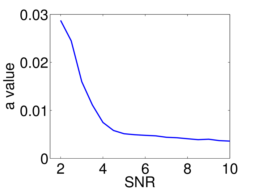
Figure 5: Impact of signal to noise ratio on value of $a$.

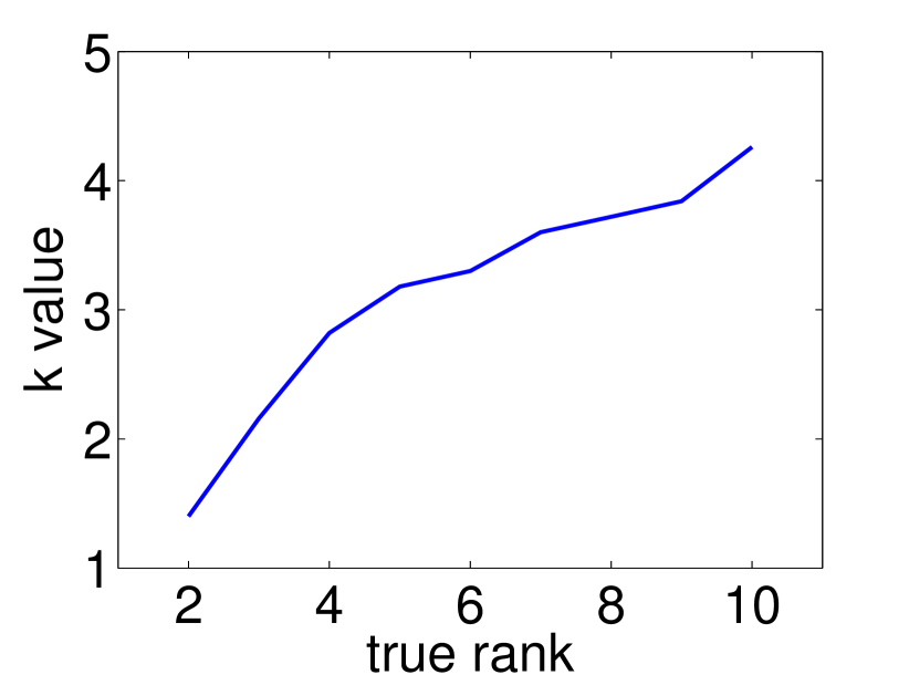
Figure 6: Impact of matrix rank on value of $k$.

Clustered Learning. We tested the centered norms on a synthetic dataset which exhibited a clustered structure. We generated a $100\times 100$, rank 5, block diagonal matrix, where the entries of each $20\times 20$ block were set to a random integer chosen uniformly in $\{1,\ldots,10\}$, with additive noise. Table 3 illustrates the results averaged over 100 runs. Within each group of norms, the box-norm and the $k$-support norm outperformed the trace norm and elastic net, and centering improved performance for all norms. Figure 7 illustrates a sample matrix along with the solution found using the box and trace norms.

Table 3: Clustered block diagonal matrix, before (left) and after (right) thresholding.

dataset	norm	test error	$r$	$k$	$a$	test error	$r$	$k$	$a$
$\rho$=10%	trace	0.6529 (0.10)	20	-	-	0.6065 (0.10)	5	-	-
	el.net	0.6482 (0.10)	20	-	-	0.6037 (0.10)	5	-	-
	k-sup	0.6354 (0.10)	19	2.72	-	0.5950 (0.10)	5	2.77	-
	box	0.6182 (0.09)	100	2.23	1.9e-2	0.5881 (0.10)	5	2.73	4.3e-3
	c-trace	0.5959 (0.07)	15	-	-	0.5692 (0.07)	5	-	-
	c-el.net	0.5910 (0.07)	14	-	-	0.5670 (0.07)	5	-	-
	c-k-sup	0.5837 (0.07)	14	2.03	-	0.5610 (0.07)	5	1.98	-
	c-box	0.5789 (0.07)	100	1.84	1.9e-3	0.5581 (0.07)	5	1.93	9.7e-3
$\rho$=15%	trace	0.3482 (0.08)	21	-	-	0.3048 (0.07)	5	-	-
	el.net	0.3473 (0.08)	21	-	-	0.3046 (0.07)	5	-	-
	k-sup	0.3438 (0.07)	21	2.24	-	0.3007 (0.07)	5	2.89	-
	box	0.3431 (0.07)	100	2.05	8.7e-3	0.3005 (0.07)	5	2.57	1.3e-3
	c-trace	0.3225 (0.07)	19	-	-	0.2932 (0.06)	5	-	-
	c-el.net	0.3215 (0.07)	18	-	-	0.2931 (0.06)	5	-	-
	c-k-sup	0.3179 (0.07)	18	1.89	-	0.2883 (0.06)	5	2.36	-
	c-box	0.3174 (0.07)	100	1.90	2.2e-3	0.2876 (0.06)	5	1.92	3.8e-3

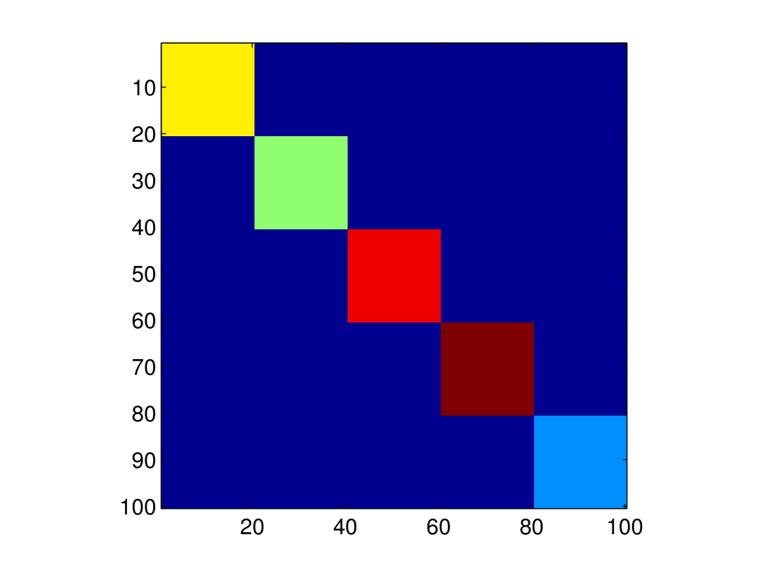
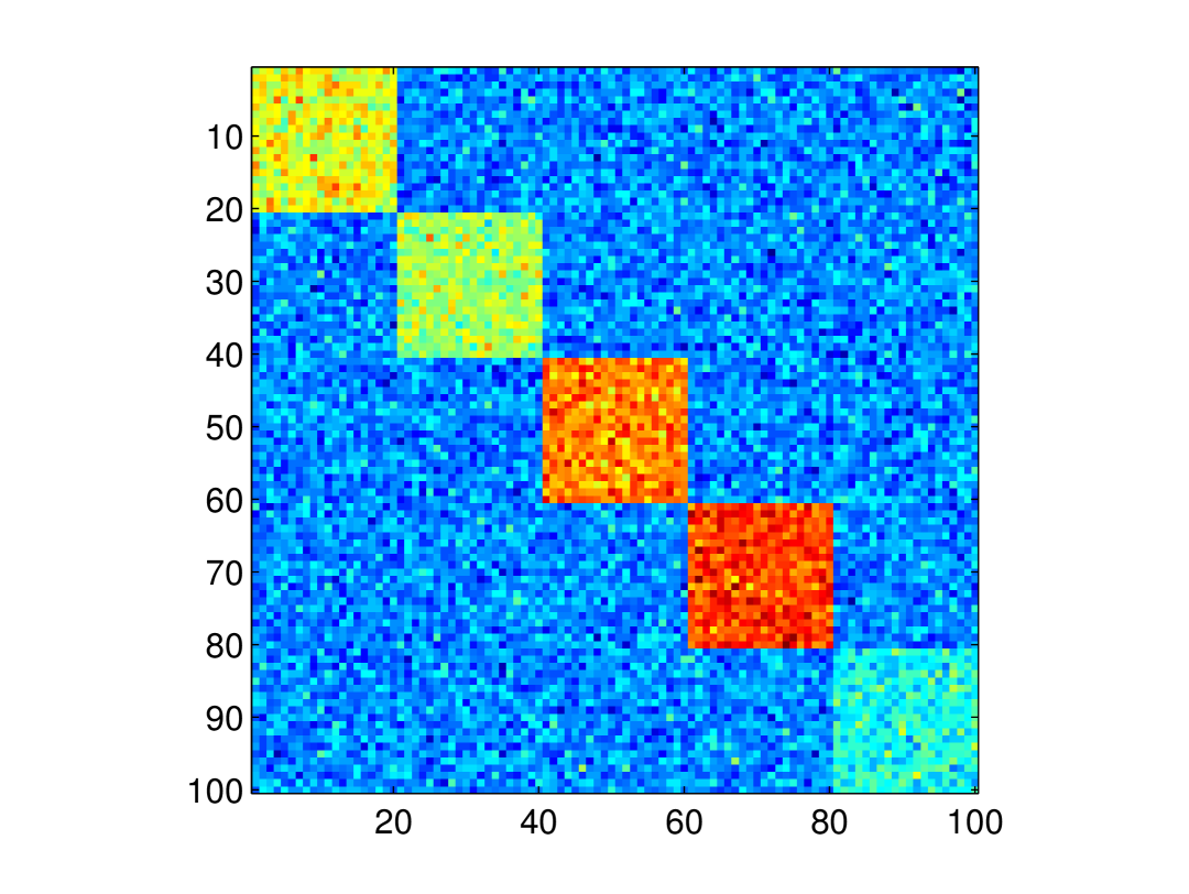
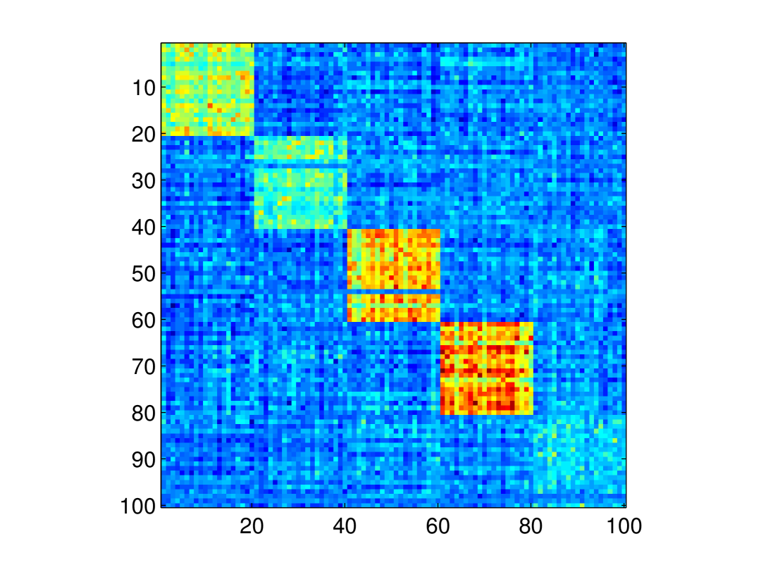
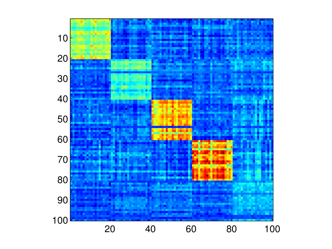
Figure 7: Clustered matrix and recovered solutions. From left to right: true, noisy, trace norm, box-norm

7.2 Real Data

Matrix Completion (MovieLens and Jester). In this section we report on the performance of the norms on real datasets. We observe a subset of the (user, rating) entries of a matrix and the task is to predict the unobserved ratings, with the assumption that the true matrix is low rank (or approximately low rank). In the first instance we considered the MovieLens datasets. These consist of user ratings of movies, the ratings are integers from 1 to 5, and all users have rated a minimum number of 20 films. Specifically we considered the following datasets:

• MovieLens 100k: 943 users and 1,682 movies, with a total of 100,000 ratings;

• MovieLens 1M: 6,040 users and 3,900 movies, with a total of 1,000,209 ratings.

We also considered the Jester datasets, which consist of user ratings of jokes, where the ratings are real values from $-10$ to $10$:

• Jester 1: 24,983 users and 100 jokes, all users have rated a minimum of 36 jokes;

• Jester 2: 23,500 users and 100 jokes, all users have rated a minimum of 36 jokes;

• Jester 3: 24,938 users and 100 jokes, all users have rated between 15 and 35 jokes.

Following Toh and Yun (2011), for MovieLens we uniformly sampled $\rho=50\%$ of the available entries for each user for training, and for Jester 1, Jester 2 and Jester 3 we sampled 20, 20 and 8 ratings per user respectively, and we again used 10% for validation. The error was measured as normalized mean absolute error,

$$\textrm{NMAE}=\frac{\|w_{\text{true}}-w_{\text{predicted}}\|^{2}}{\#\text{observations}/(r_{\max}-r_{\min})},$$

where $r_{\max}$ and $r_{\min}$ are upper and lower bounds for the ratings (Toh and Yun, 2011), averaged over 50 runs. The results are outlined in Table 4. In the thresholding case, the spectral box-norm and the spectral $k$-support norm showed the best performance, and in the absence of thresholding, the spectral $k$-support norm showed slightly improved performance. Comparing to the synthetic datasets, this suggests that the parameter $a$ did not provide any benefit in the absence of noise. We also note that without thresholding our results for trace norm regularization on MovieLens 100k agreed with those in Jaggi and Sulovsky (2010).

Table 4: Matrix completion on real datasets, without (left) and with (right) thresholding.

dataset	norm	test error	$r$	$k$	$a$	test error	$r$	$k$	$a$
MovieLens	trace	0.2034	87	-	-	0.2017	13	-	-
100k	el.net	0.2034	87	-	-	0.2017	13	-	-
$\rho=50\%$	k-sup	0.2031	102	1.00	-	0.1990	9	1.87	-
	box	0.2035	943	1.00	1e-5	0.1989	10	2.00	1e-5
MovieLens	trace	0.1821	325	-	-	0.1790	17	-	-
1M	el.net	0.1821	319	-	-	0.1789	17	-	-
$\rho=50\%$	k-sup	0.1820	317	1.00	-	0.1782	17	1.80	-
	box	0.1817	3576	1.09	3e-5	0.1777	19	2.00	1e-6
Jester 1	trace	0.1787	98	-	-	0.1752	11	-	-
20 per line	el.net	0.1787	98	-	-	0.1752	11	-	-
	k-sup	0.1764	84	5.00	-	0.1739	11	6.38	-
	box	0.1766	100	4.00	1e-6	0.1726	11	6.40	2e-5
Jester2	trace	0.1767	98	-	-	0.1758	11	-	-
20 per	el.net	0.1767	98	-	-	0.1758	11	-	-
line	k-sup	0.1762	94	4.00	-	0.1746	11	4.00	-
	box	0.1762	100	4.00	2e-6	0.1745	11	4.50	5e-5
Jester 3	trace	0.1988	49	-	-	0.1959	3	-	-
8 per line	el.net	0.1988	49	-	-	0.1959	3	-	-
	k-sup	0.1970	46	3.70	-	0.1942	3	2.13	-
	box	0.1973	100	5.91	1e-3	0.1940	3	4.00	8e-4

Multitask Learning (Lenk and Animals with Attributes). In our final set of experiments we considered two multitask learning datasets, where we expected the data to exhibit clustering. The Lenk personal computer dataset (Lenk et al., 1996) consists of 180 ratings of 20 profiles of computers characterized by 14 features (including a bias term). The clustering is suggested by the assumption that users are motivated by similar groups of features. We used the root mean square error of true vs. predicted ratings, normalised over the tasks, averaged over 100 runs. We also report on the Frobenius norm, which in the multitask learning framework corresponds to independent task learning. The results are outlined in Table 5. The centered versions of the spectral $k$-support norm and spectral box-norm outperformed the other penalties in all regimes. Furthermore, the results clearly indicate the importance of centering, as discussed for the trace norm in Evgeniou et al. (2007).

Table 5: Multitask learning clustering on Lenk dataset.

norm	test error	$k$	$a$
fr	3.7931 (0.07)	-	-
trace	1.9056 (0.04)	-	-
el.net	1.9007 (0.04)	-	-
k-sup	1.8955 (0.04)	1.02	-
box	1.8923 (0.04)	1.01	5.5e-3
c-fr	1.8634 (0.08)	-	-
c-trace	1.7902 (0.03)	-	-
c-el.net	1.7897 (0.03)	-	-
c-k-sup	1.7777 (0.03)	1.89	-
c-box	1.7759 (0.03)	1.12	8.6e-3

The Animals with Attributes dataset (Lampert et al., 2009) consists of 30,475 images of animals from 50 classes. Along with the images, the dataset includes pre-extracted features for each image. The dataset has been analyzed in the context of multitask learning. We followed the experimental protocol from (Kang et al., 2011), however we used an updated feature set, and we considered all 50 classes. Specifically, we used the DeCAF feature set provided by Lampert et al. (2009) rather than the SIFT bag of word descriptors. These updated features were obtained through a deep convolutional network and represent each image by a 4,096-dimensional vector (Donahue et al., 2014). As the smallest class size is 92 we selected the first $n=92$ examples of each of the $T=50$ classes, used PCA (with centering) on the resulting data matrix to reduce dimensionality ($d=1,718$) retaining a variance of 95%, and obtained a dataset of size $4,600\times 1,718$. For each class the examples were split into training, validation and testing datasets, with a split of 50%, 25%, 25% respectively, and we averaged the performance over 50 runs.

We used the logistic loss, yielding the error term

$${\cal L}(W)=\sum_{t=1}^{T}\sum_{i=1}^{Tn}\log\left(1+\exp(-y_{t,i}\langle w_{t},x_{i}\rangle)\right)$$

where $W=[w_{1},\ldots,w_{T}]$, $x_{1},\ldots,x_{Tn}$ are the inputs and $y_{t,i}=1$ if $x_{i}$ is in class $t$, and $y_{t,i}=-1$ otherwise.

The predicted class for testing example $x$ was $\operatorname*{\arg\!\max}_{t=1}^{T}\langle w_{t},x\rangle$ and the accuracy was measured as the percentage of correctly classified examples, also known as multi-class error. The results without centering are outlined in Table 6. The corresponding results with centering showed the same relative performance, but worse overall accuracy, which is reasonable as the data is not expected to be clustered, and we omit the results here.

The spectral $k$-support and box-norms gave the best results, outperforming the Frobenius norm and the matrix elastic net, which in turn outperformed the trace norm. We highlight that in contrast to the Lenk experiments, the Frobenius norm, corresponding to independent task learning, was competitive. Furthermore, the optimal values of $k$ for the spectral $k$-support norm and spectral box-norm were high (38 and 33, respectively) relative to the maximum rank of 50, corresponding to a relatively high rank solution. The spectral $k$-support norm and spectral box-norm nonetheless outperformed the other regularizers. Notice also that the spectral $k$-support norm requires the same number of parameters to be tuned as the matrix elastic net, which suggests that it somehow captures the underlying structure of the data in a more appropriate manner.

We finally note as an aside that using the SIFT bag of words descriptors provided by Lampert et al. (2009), which represent the images as a $2,000$-dimensional histogram of local features, we replicated the results for independent task learning (Frobenius norm regularization) and single-group learning (trace norm regularization) of Kang et al. (2011) for the subset of 20 classes considered in their paper.

Table 6: Multitask learning clustering on Animals with Attributes dataset, no centering.

norm	test error	$k$	$a$
fr	38.3428 (0.74)	-	-
tr	37.4285 (0.76)	-	-
el.net	38.2857 (0.73)	-	-
k-sup	38.8571 (0.71)	37.8	-
box	38.9100 (0.65)	32.8	2.1e-2

8 Extensions

In this section we outline a number of extensions to topics in this paper.

8.1 $k$-Support $p$-Norms

A natural extension of the $k$-support norm follows by applying a $p$-norm, rather than the Euclidean norm, in the infimum convolution definition of the $k$-support norm. In the dual norm, we then obtain the corresponding $q$-norm, where $\frac{1}{p}+\frac{1}{q}=1$.

Definition 21

The $k$-support $p$-norm is defined for $w\in{\mathbb{R}}^{d}$ as

$$\|w\|_{(k,p)} =\operatorname*{\vphantom{p}inf}\left\{\sum_{g\in{\cal G}_{k}}\|v_{g}\|_{p}:\operatorname{supp}(v_{g})\subseteq g,\sum_{g\in{\cal G}_{k}}v_{g}=w\right\}.$$ (35)

The following corollary follows along the same lines as the proof of Proposition 3 in the appendix.

Corollary 22

The $(p,k)$-support norm is well defined and its unit ball is the convex hull of the set $\{w\in{\mathbb{R}}^{d}:\|w\|_{p}\leq 1,~{}{\rm card}(w)\leq k\}$. Furthermore, its dual norm is given by

$$\|u\|_{*,(k,q)}=\left(\sum_{i=1}^{k}(|u|^{\downarrow}_{i})^{q}\right)^{\frac{1}{q}},~{}~{}~{}u\in{\mathbb{R}}^{d}.$$

We discuss the special cases $p\in\{1,2,\infty\}$. The case $p=2$ is the $k$-support norm of Argyriou et al. (2012) discussed above. For $p=1$ we have $\|u\|_{*,(k,q)}=\|u\|_{\infty}$, hence the $(k,1)$-support norm coincides with the $\ell_{1}$ norm for every $k\in{{\mathbb{N}}}_{d}$. The case $p=\infty$ is more interesting; specifically the dual norm is the well-known Ky-Fan norm (see e.g. Bhatia, 1997).

$$\|u\|_{*,(k,\infty)}=\sum_{i=1}^{k}|u|^{\downarrow}_{i}.$$

Using the fact that the primal norm is the dual of the dual, we obtain by a direct computation that

$$\|w\|_{(k,\infty)}=\max\left(\|w\|_{\infty},\frac{1}{k}\|w\|_{1}\right).$$

It is clear that the $(p,k)$-support norm is a symmetric gauge function. Hence we we can define the spectral $(p,k)$-support norm as $\|W\|_{(k,p)}=\|\sigma(W)\|_{(k,p)}$, for $W\in{\mathbb{R}}^{d\times T}$. Since the dual of any orthogonally invariant norm is given by $\|\cdot\|_{*}=\|\sigma(\cdot)\|_{*}$ (see e.g. Lewis, 1995), we conclude that the dual spectral $(k,p)$-support norm is given by $\|U\|_{*,(k,p)}=\|\sigma(U)\|_{*,(k,p)}$, for every $U\in{\mathbb{R}}^{d\times T}$. Furthermore, the unit ball of the spectral $(p,k)$-support norm is equal to the convex hull of the set $\{W\in{\mathbb{R}}^{d\times T}:{\rm rank}(W)\leq k,\,\|\sigma(W)\|_{p}\leq 1\}$.

8.2 Kernels

The ideas discussed in this paper can be used in the context of multiple kernel learning in a natural way (see e.g. Micchelli and Pontil, 2007, and references therein). Let $K_{j}$, $j\in{\mathbb{N}}_{s}$, be prescribed reproducing kernels on a set $X$ , and $H_{j}$ the corresponding reproducing kernel Hilbert spaces with norms $\|\cdot\|_{j}$. We consider the problem

$$\min\left\{\sum_{i=1}^{n}\ell\Big{(}y_{i},\sum_{\ell=1}^{s}f_{\ell}(x_{i})\Big{)}+\lambda\big{\|}\big{(}\|f_{1}\|_{1},\dots,\|f_{s}\|_{s}\big{)}\big{\|}_{\Theta}^{2}:f_{1}\in H_{1},\dots,f_{s}\in H_{s}\right\}.$$

The choice $\Theta=\{\theta\in{\mathbb{R}}^{d}:0<\theta_{i}\leq 1,~{}\sum_{i=1}^{d}\theta_{i}\leq k\}$, when $k\leq s$, is particularly interesting. It gives rise to a version of multiple kernel learning in which at least $k$ kernels are employed.

8.3 Rademacher complexity

We briefly comment on the Rademacher complexity of the spectral $k$-support norm, namely

$${\mathbb{E}}\operatorname*{\vphantom{p}sup}_{\|W\|_{(k)}\leq 1}\frac{1}{Tn}\sum_{t=1}^{T}\sum_{i=1}^{n}\epsilon_{i}^{t}{\langle}w_{t},x_{i}^{t}{\rangle}$$

where the expectations is taken with respect to i.i.d. Rademacher random variables $\epsilon_{i}^{t}$, $i\in{\mathbb{N}}_{n},~{}t\in{\mathbb{N}}_{T}$ and the $x_{i}^{t}$ are either prescribed or random datapoints associated with the different regression tasks. The Rademacher complexity can be used to derive uniform bounds on the estimation error and excess risk bounds (see Bartlett and Mendelson, 2002; Koltchinskii and Panchenko, 2002, for a discussion). Although a complete analysis is beyond the scope of the present paper, we remark that the Rademacher complexity of the unit ball of the spectral $k$-support is a factor of $\sqrt{k}$ larger than the Rademacher complexity bound for the trace norm provided in (Proposition 6 Maurer and Pontil, 2013). This follows from the fact that the dual spectral $k$-support norm is bounded by $\sqrt{k}$ times the operator norm. Of course the unit ball of the spectral $k$-support norm contains the unit ball of the trace norm, so the associated excess risk bounds need to be compared with care.

9 Conclusion

We studied the family of box-norms, and showed that the $k$-support norm belongs to this family. We noted that these can be naturally extended from the vector to the matrix setting. We also provided a connection between the $k$-support norm and the cluster norm, which essentially coincides with the spectral box-norm. We further observed that the cluster norm is a perturbation of the spectral $k$-support norm, and we were able to compute the norm and the proximity operator of the squared norm. We also provided a method to solve regularization problems using centered versions of the norms and we considered a number of extensions to the box-norm framework.

Our experiments indicate that the spectral box-norm and $k$-support norm consistently outperform the trace norm and the matrix elastic net on various matrix completion problems. Furthermore, we studied the application of centering to clustering problems in multitask learning, and found that this improved performance. With a single parameter, compared to two for the spectral box-norm, and three for the cluster norm, our results suggest that the spectral $k$-support norm represents a powerful yet straightforward alternative to the trace norm for low rank matrix learning. In future work we would like to complete the analysis of the Rademacher complexity for the norms in this paper, and derive associated statistical oracle inequalities. We would also like to investigate the family of $\Theta$-norms for more general parameter sets.

Acknowledgments

We would like to thank Andreas Maurer, Charles Micchelli and especially Andreas Argyriou for useful discussions. This work was supported in part by EPSRC Grant EP/H027203/1.

A

In this appendix, we discuss some auxiliary results which are used in the main body of the paper.

Let $X$ be a finite dimensional vector space. Recall that a subset $C$ of $X$ is called balanced if $\alpha C\subseteq C$ whenever $|\alpha|\leq 1$. Furthermore, $C$ is called absorbing if for any $x\in X$, $x\in\lambda C$ for some $\lambda>0$.

Lemma 23

Let $C\subseteq X$ be a bounded, convex, balanced, and absorbing set. The Minkowski functional $\mu_{C}$ of $C$, defined, for every $w\in X$, as

$$\mu_{C}(w)=\operatorname*{\vphantom{p}inf}\left\{\lambda:\lambda>0,~{}\frac{1}{\lambda}w\in C\right\}$$

is a norm on $X$.

Proof  We give a direct proof that $\mu_{C}$ satisfies the properties of a norm. See also e.g. (Rudin, 1991, §1.35) for further details. Clearly $\mu_{C}(w)\geq 0$ for all $w$, and $\mu_{C}(0)=0$. Moreover, as $C$ is bounded, $\mu_{C}(w)>0$ whenever $w\neq 0$.

Next we show that $\mu_{C}$ is one-homogeneous. For every $\alpha\in{\mathbb{R}}$, $\alpha\neq 0$, let $\sigma={\rm sign}(\alpha)$ and note that

$$\mu_{C}(\alpha w) =\operatorname*{\vphantom{p}inf}\left\{\lambda>0:\frac{1}{\lambda}\alpha w\in C\right\}$$

$$=\operatorname*{\vphantom{p}inf}\left\{\lambda>0:\frac{|\alpha|}{\lambda}\sigma w\in C\right\}$$

$$=|\alpha|\operatorname*{\vphantom{p}inf}\left\{\lambda>0:\frac{1}{\lambda}w\in\sigma C\right\}$$

$$=|\alpha|\operatorname*{\vphantom{p}inf}\left\{\lambda>0:\frac{1}{\lambda}w\in C\right\}=|\alpha|\mu_{C}(w),$$

where we have made a change of variable and used the fact that $\sigma C=C$.

Finally, we prove the triangle inequality. For every $v,w\in X$, if $v/{\lambda}\in C$ and $w/\mu\in C$ then setting $\gamma={\lambda}/({\lambda}+\mu)$, we have

$$\frac{v+w}{{\lambda}+\mu}=\gamma\frac{v}{{\lambda}}+(1-\gamma)\frac{w}{\mu}$$

and since $C$ is convex, then $\frac{v+w}{{\lambda}+\mu}\in C$. We conclude that $\mu_{C}(v+w)\leq\mu_{C}(v)+\mu_{C}(w)$. The proof is completed.  
Note that for such set $C$, the unit ball of the induced norm $\mu_{C}$ is $C$. Furthermore, if $\|\cdot\|$ is a norm then its unit ball satisfies the hypotheses of Lemma 23.

Using this lemma we can prove Proposition 3.

Proof of Proposition 3 Let $A_{{\ell}}=\{w\in{\mathbb{R}}^{d}:\|w\|_{\gamma^{\ell}}\leq 1,~{}\operatorname{supp}(w)\subseteq\operatorname{supp}(\gamma^{\ell})\}$, and define

$$C={\rm co}\bigcup\limits_{\ell=1}^{m}A_{\ell}.$$

Note that $C$ is bounded and balanced, since each set $A_{\ell}$ is so. Furthermore, the hypothesis that $\sum_{\ell=1}^{m}\gamma^{\ell}>0$ ensures that $C$ is absorbing. Hence, by Lemma 23 the Minkowski functional $\mu_{C}$ defines a norm. We rewrite $\mu_{C}(w)$ as

$$\mu_{C}(w)=\operatorname*{\vphantom{p}inf}\left\{\lambda:\lambda>0,~{}w=\lambda\sum_{{\ell}=1}^{m}\alpha_{{\ell}}z_{\ell},~{}z_{\ell}\in A_{{\ell}},~{}\alpha\in\Delta^{m-1}\right\}$$

where the infimum is over $\lambda$, the vectors $z_{\ell}\in{\mathbb{R}}^{d}$ and the vector $\alpha=(\alpha_{1},\dots,\alpha_{m})$, and recall $\Delta^{m-1}$ denotes the unit simplex in ${\mathbb{R}}^{m}$.

The rest of the proof is structured as follows. We first show that $\mu_{C}(w)$ coincides with the right hand side of equation (3), which we denote by $\nu(w)$. Then we show that $\|w\|_{\Theta}=\mu_{C}(w)$ by observing that both norms have the same dual norm.

Choose any vectors $v_{1},\dots,v_{m}\in{\mathbb{R}}^{d}$ which satisfies the constraint set in the right hand side of (3) and set $\alpha_{\ell}=\|v_{{\ell}}\|_{\gamma^{{\ell}}}/(\sum_{k=1}^{m}\|v_{k}\|_{\gamma^{k}})$ and $z_{\ell}=v_{\ell}/\|v_{\ell}\|_{\gamma^{\ell}}$. We have

$$w=\sum_{{\ell}=1}^{m}v_{{\ell}}=\Big{(}\sum_{k=1}^{m}\|v_{k}\|_{\gamma^{k}}\Big{)}\sum_{{\ell}=1}^{m}\alpha_{{\ell}}z_{{\ell}}.$$

This implies that $\mu_{C}(w)\leq\nu(w)$. Conversely, if $w=\lambda\sum_{\ell=1}^{m}\alpha_{\ell}z_{\ell}$ for some $z_{\ell}\in A_{\ell}$ and $\alpha\in\Delta^{m-1}$, then letting $v_{\ell}=\lambda\alpha_{\ell}z_{\ell}$ we have

$$\sum_{{\ell}=1}^{m}\|v_{{\ell}}\|_{\gamma^{{\ell}}} =\sum_{{\ell}=1}^{m}\|\lambda\alpha_{{\ell}}z_{{\ell}}\|_{\gamma^{{\ell}}}=\lambda\sum_{{\ell}=1}^{m}\alpha_{{\ell}}\|z_{{\ell}}\|_{\gamma^{{\ell}}}\leq\lambda.$$

Next, we show that both norms have the same dual norm. We noted in Proposition 2 that the dual norm of $\|\cdot\|_{\Theta}$ takes the form (2). When $\Theta$ is the interior of ${\rm co}\{\gamma^{1},\dots,\gamma^{m}\}$, this can be written as

$$\|u\|_{*,\Theta}=\operatorname*{\vphantom{p}sup}_{\theta\in\Theta}\sqrt{\sum_{i=1}^{d}\theta_{i}u_{i}^{2}}=\max_{{\ell}=1}^{m}\sqrt{\sum_{i=1}^{d}\gamma^{\ell}_{i}u_{i}^{2}}.$$

We now compute the dual of the norm $\mu_{C}$,

$$\max_{w\in C}{\langle}w,u{\rangle}=\max\left\{{\langle}w,u{\rangle}:w\in\cup_{{\ell}=1}^{m}A_{{\ell}}\right\}=\max_{{\ell}=1}^{m}\max_{w\in A_{{\ell}}}{\langle}w,u{\rangle}=\max_{{\ell}=1}^{m}\sqrt{\sum_{i=1}^{d}\gamma^{\ell}_{i}u_{i}^{2}}.$$ (36)

It follows that the norms share the same dual norm, hence $\mu_{C}(\cdot)$ coincides with $\|\cdot\|_{\Theta}$.  

The above proof reveals that the unit ball of the dual norm of $\|\cdot\|_{\Theta}$ is given by an intersection of ellipsoids in ${\mathbb{R}}^{d}$. Indeed equation (36) provides that

$$\left\{u\in{\mathbb{R}}^{d}:\|u\|_{*,\Theta}\leq 1\right\} =\left\{u\in{\mathbb{R}}^{d}:\max_{{\ell}=1}^{m}\sum_{i=1}^{d}\gamma^{\ell}_{i}u_{i}^{2}\leq 1\right\}$$

$$=\left\{u\in{\mathbb{R}}^{d}:\sum_{i=1}^{d}\gamma^{\ell}_{i}u_{i}^{2}\leq 1,\forall{\ell}\in{{\mathbb{N}}}_{m}\right\}$$

$$=\bigcap_{{\ell}\in{{\mathbb{N}}}_{m}}\left\{u\in{\mathbb{R}}^{d}:\sum_{i=1}^{d}\gamma^{\ell}_{i}u_{i}^{2}\leq 1\right\}.$$ (37)

Notice that for each ${\ell}\in{{\mathbb{N}}}_{m}$, the set $\left\{u\in{\mathbb{R}}^{d}:\sum_{i=1}^{d}\gamma^{\ell}_{i}u_{i}^{2}\leq 1\right\}$ defines a (possibly degenerate) ellipsoid in $X$, where the $i$-th semi-principal axis has length $1/\sqrt{\gamma^{\ell}_{i}}$ (which is infinite if $\gamma^{\ell}_{i}=0$) and the unit ball of the dual $\Theta$-norm is given by the intersection of $m$ such ellipsoids.

The following result, which is discussed in (Argyriou et al., 2012, Section 2) is key for the proof of Proposition 18.

Corollary 24

The unit ball of the vector $k$-support norm is equal to the convex hull of the set $\{w\in\mathbb{R}^{d}:{\rm card}(w)\leq k,\|w\|_{2}\leq 1\}$.

Proof  The result follows directly by Corollary 4 for ${\cal G}={\cal G}_{k}$ observing that in this case $\bigcup_{g\in{\cal G}_{k}}\left\{w\in{\mathbb{R}}^{d}:\operatorname{supp}(w)\subseteq g,\|w\|_{2}\leq 1\right\}=\{w\in{\mathbb{R}}^{d}:{\rm card}(w)\leq k,\|w\|_{2}\leq 1\}$.  

The next result is due to Von Neumann (1937); see also Lewis (1995).

Theorem 25 (Von Neumann’s trace inequality)

For any $d\times m$ matrices $X$ and $Y$,

$${\rm tr}(XY^{\scriptscriptstyle\top})\leq\langle\sigma(X),\sigma(Y)\rangle$$

and equality holds if and only if $X$ and $Y$ admit a simultaneous singular value decomposition, that is, $X=U{\rm diag}(\sigma(X))V^{\scriptscriptstyle\top}$, $Y=U{\rm diag}(\sigma(Y))V^{\scriptscriptstyle\top}$, where $U\in\mathbb{R}^{d\times d}$ and $V\in\mathbb{R}^{m\times m}$ are orthogonal matrices.

The following inequality is given in Marshall and Olkin (1979, Sec. 9 H.1.h).

Lemma 26

If $A,B\in{\bf S}^{d}_{+}$, then it holds

$${\rm tr}(AB)=\sum_{i=1}^{d}\lambda_{i}(AB)\geq\sum_{i=1}^{d}\lambda_{i}(A)\lambda_{d-i+1}(B).$$

References

- Abernethy et al. (2009) J. Abernethy, F. Bach, T. Evgeniou, and J.-P. Vert. A new approach to collaborative filtering. Journal of Machine Learning Research, 10:803–826, 2009.
- Aflalo et al. (2011) J. Aflalo, A. Ben-Tal, C. Bhattacharyya, J. S. Nath, and S. Raman. Variable sparsity kernel learninig. JMLR, 12:565–592, 2011.
- Argyriou et al. (2007) A. Argyriou, T. Evgeniou, and M. Pontil. Multi-task feature learning. Advances in Neural Information Processing Systems 19, pages 41–48, 2007.
- Argyriou et al. (2008) A. Argyriou, T. Evgeniou, and M. Pontil. Convex multi-task feature learning. Machine Learning, 73(3):243–272, 2008.
- Argyriou et al. (2011) A. Argyriou, C. A. Micchelli, M. Pontil, L. Shen, and Y. Xu. Efficient first order methods for linear composite regularizers. CoRR, abs/1104.1436, 2011.
- Argyriou et al. (2012) A. Argyriou, R. Foygel, and N. Srebro. Sparse prediction with the k-support norm. Advances in Neural Information Processing Systems 25, pages 1466–1474, 2012.
- Bach et al. (2011) F. Bach, R. Jenatton, J. Mairal, and G. Obozinski. Optimization with sparsity-inducing penalties. Foundations and Trends in Mach. Learn., 4(1):1–106, 2011.
- Bartlett and Mendelson (2002) P. L. Bartlett and S. Mendelson. Rademacher and gaussian complexities: Risk bounds and structural results. Journal of Machine Learning Research, 3:463–482, 2002.
- Bauschke and Combettes (2010) H. H. Bauschke and P. L. Combettes. Convex Analysis and Monotone Operator Theory in Hilbert Spaces. Canadian Mathematical Society, 2010.
- Beck and Teboulle (2009) A. Beck and M. Teboulle. A fast iterative shrinkage-thresholding algorithm for linear inverse problems. SIAM J. Imaging Sciences, 2(1):183–202, 2009.
- Bertsekas et al. (2003) D. P. Bertsekas, A. Nedic, and A. E. Ozdaglar. Convex Analysis and Optimization. Athena Scientific, 2003.
- Bhatia (1997) R. Bhatia. Matrix Analysis. Springer, 1997.
- Boyd and Vandenberghe (2004) S. Boyd and L. Vandenberghe. Convex Optimization. Cambridge University Press, 2004.
- Cavallanti et al. (2010) G. Cavallanti, N. Cesa-Bianchi, and C. Gentile. Linear algorithms for online multitask classification. Journal of Machine Learning Research, 1:2901–2934, 2010.
- Chatterjee et al. (2014) S. Chatterjee, S. Chen, and A. Banerjee. Generalized Dantzig selector: application to the k-support norm. In Advances in Neural Information Processing Systems 28, 2014.
- Combettes and Pesquet (2011) P. L. Combettes and J.-C. Pesquet. Proximal splitting methods in signal processing. In Fixed-Point Algorithms for Inverse Problems. Springer, 2011.
- Donahue et al. (2014) J. Donahue, Y. Jia, O. Vinyals, J. Hoffman, N. Zhang, E. Tzeng, and T. Darrell. DeCAF: A Deep Convolutional Activation Feature for Generic Visual Recognition. In Proceedings of the 31st International Conference on Machine Learning, 2014.
- Evgeniou et al. (2005) T. Evgeniou, C. A. Micchelli, and M. Pontil. Learning multiple tasks with kernel methods. Journal of Machine Learning Research, 6:615–637, 2005.
- Evgeniou et al. (2007) T. Evgeniou, M. Pontil, and O. Toubia. A convex optimization approach to modeling heterogeneity in conjoint estimation. Marketing Science, 26:805–818, 2007.
- Gkirtzou et al. (2013) K. Gkirtzou, J. Honorio, D. Samaras, R. Goldstein, and M. B. Blaschko. fMRI analysis of cocaine addiction using k-support sparsity. In International Symposium on Biomedical Imaging, 2013.
- Grandvalet (1998) Y. Grandvalet. Least absolute shrinkage is equivalent to quadratic penalization. In ICANN 98, pages 201–206. Springer London, 1998.
- Jacob et al. (2009a) L. Jacob, F. Bach, and J.-P. Vert. Clustered multi-task learning: a convex formulation. Advances in Neural Information Processing Systems 21, 2009a.
- Jacob et al. (2009b) L. Jacob, G. Obozinski, and J.-P. Vert. Group lasso with overlap and graph lasso. Proceedings of the 26th International Conference on Machine Learning, 2009b.
- Jaggi and Sulovsky (2010) M Jaggi and M. Sulovsky. A simple algorithm for nuclear norm regularized problems. Proceedings of the 27th International Conference on Machine Learning, 2010.
- Kang et al. (2011) Z. Kang, K. Grauman, and F. Sha. Learning with whom to share in multi-task feature learning. In Proceedings of the 28th International Conference on Machine Learning, 2011.
- Koltchinskii and Panchenko (2002) V. Koltchinskii and D. Panchenko. Empirical margin distributions and bounding the generalization error of combined classifiers. The Annals of Statistics, 30(1):1–50, 2002.
- Lampert et al. (2009) C. H. Lampert, H. Nickisch, and S. Harmeling. Learning to detect unseen object classes by between-class attribute transfer. In IEEE Computer Vision and Pattern Recognition (CVPR), 2009.
- Lenk et al. (1996) P. J. Lenk, W. S. DeSarbo, P. E. Green, and M. R. Young. Hierarchical bayes conjoint analysis: Recovery of partworth heterogeneity from reduced experimental designs. Marketing Science, 15(2):173–191, 1996.
- Lewis (1995) A. S. Lewis. The convex analysis of unitarily invariant matrix functions. Journal of Convex Analysis, 2:173–183, 1995.
- Li et al. (2012) H. Li, N. Chen, and L. Li. Error analysis for matrix elastic-net regularization algorithms. IEEE Transactions on Neural Networks and Learning Systems, 23-5:737–748, 2012.
- Marshall and Olkin (1979) A. W. Marshall and I. Olkin. Inequalities: Theory of Majorization and its Applications. Academic Press, 1979.
- Maurer (2006) A. Maurer. Bounds for linear multi-task learning. JMLR, 2006.
- Maurer and Pontil (2008) A. Maurer and M. Pontil. A uniform lower error bound for half-space learning. ALT, 2008.
- Maurer and Pontil (2012) A. Maurer and M. Pontil. Structured sparsity and generalization. The Journal of Machine Learning Research, 13:671–690, 2012.
- Maurer and Pontil (2013) A. Maurer and M. Pontil. Excess risk bounds for multitask learning with trace norm regularization. In Proceedings of The 27th Conference on Learning Theory (COLT), 2013.
- Mazumder et al. (2010) R. Mazumder, T. Hastie, and R. Tibshirani. Spectral regularization algorithms for learning large incomplete matrices. Journal of Machine Learning Research, 11:2287–2322, 2010.
- McDonald et al. (2014) A. M. McDonald, M. Pontil, and D. Stamos. Spectral k-support regularization. In Advances in Neural Information Processing Systems 28, 2014.
- Micchelli and Pontil (2005) C. A. Micchelli and M. Pontil. Learning the kernel function via regularization. Journal of Machine Learning Research, 6:1099–1125, 2005.
- Micchelli and Pontil (2007) C. A. Micchelli and M. Pontil. Feature space perspectives for learning the kernel. Machine Learning, 66:297–319, 2007.
- Micchelli et al. (2010) C. A. Micchelli, J. M. Morales, and M. Pontil. A family of penalty functions for structured sparsity. Advances in Neural Information Processing Systems 23, 2010.
- Micchelli et al. (2013) C. A. Micchelli, J. M. Morales, and M. Pontil. Regularizers for structured sparsity. Advances in Comp. Mathematics, 38:455–489, 2013.
- Nesterov (2007) Y. Nesterov. Gradient methods for minimizing composite objective function. Center for Operations Research and Econometrics, 76, 2007.
- Obozinski and Bach (2012) G. Obozinski and F. Bach. Convex relaxation for combinatorial penalties. CoRR, 2012.
- Rockafellar (1970) R. T. Rockafellar. Convex Analysis. Princeton University Press, 1970.
- Rockafellar and Wets (2009) R. T. Rockafellar and R. J.-B. Wets. Variational Analysis. Springer, 2009.
- Rudin (1991) W. Rudin. Functional Analysis. McGraw Hill, 1991.
- Srebro et al. (2005) N. Srebro, J. D. M. Rennie, and T. S. Jaakkola. Maximum-margin matrix factorization. Advances in Neural Information Processing Systems 17, 2005.
- Szafranski et al. (2007) M. Szafranski, Y. Grandvalet, and P. Morizet-Mahoudeaux. Hierarchical penalization. In Advances in Neural Information Processing Systems 21, 2007.
- Tibshirani (1996) R. Tibshirani. Regression shrinkage and selection via the lasso. Journal of the Royal Statistical Society, 58:267–288, 1996.
- Toh and Yun (2011) K.-C. Toh and S. Yun. An accelerated proximal gradient algorithm for nuclear norm regularized least squares problems. SIAM J. on Img. Sci., 4:573–596, 2011.
- Von Neumann (1937) J. Von Neumann. Some matrix-inequalities and metrization of matric-space. Tomsk. Univ. Rev. Vol I, 1937.
- Zou and Hastie (2005) H. Zou and T. Hastie. Regularization and variable selection via the elastic net. Journal of the Royal Statistical Society, Series B, 67(2):301–320, 2005.