Role of the kinematics of probing electrons in electron energy-loss spectroscopy of solid surfaces

Abstract

Inelastic scattering of electrons incident on a solid surface is determined by the two properties: (i) electronic response of the target system and (ii) the detailed quantum-mechanical motion of the projectile electron inside and in the vicinity of the target. We emphasize the equal importance of the second ingredient, pointing out the fundamental limitations of the conventionally used theoretical description of the electron energy-loss spectroscopy (EELS) in terms of the “energy-loss functions”. Our approach encompasses the dipole and impact scattering as specific cases, with the emphasis on the quantum-mechanical treatment of the probe electron. Applied to the high-resolution EELS of Ag surface, our theory largely agrees with recent experiments, while some instructive exceptions are rationalized.

I Introduction

Electron energy-loss spectroscopy (EELS) is an efficient and widely used experimental method to study excitation processes on clean and adsorbates-covered surfaces of solids, and in thin (including atomically thin) films Hillier and Baker (1944); Ibach and Mills (1982); Eberlein et al. (2008); Egerton (2009). This method utilizes the inelastic scattering of electrons, resulting in both the energy and momentum transfer from the projectiles to diverse kinds of excitations in the samples. Reflected or transmitted electrons are analyzed with respect to the energy and momentum loss they have experienced in the interaction with a target, revealing a wealth of information about the properties of the latter.

Much efforts have been exerted over years to complement EELS experimental techniques with comprehensive theoretical pictures Pines and Nozieres (1966); Ritchie (1957); Bennett (1970); Ibach and Mills (1982); Tsuei et al. (1990); Liebsch (1998, 1997); Nazarov (2015). In this way, a clear understanding of elementary excitations (such as electron-hole pairs generation, collective electronic excitations – plasmons, atomic vibrational modes, etc.), including their momentum dispersion, for solid surfaces, interfaces, and in thin films have been achieved.

Presently, the main approach to interpret EELS data theoretically is to use energy-loss functions. A clear example is the surface energy-loss function of a semi-infinite solid, which, with the neglect of the momentum dispersion, can be written as Liebsch (1997)

$$L_{s}(\omega)=-\text{Im}\frac{1}{\varepsilon(\omega)+1},$$ (1)

where $\varepsilon(\omega)$ is the frequency-dependent dielectric function (DF) of the bulk solid. This example exhibits an important feature common also to other, much more sophisticated, loss-functions: $L_{s}(\omega)$ of Eq. (1) is a property of the target only. Indeed, it is not concerned with the setup of the EELS experiment, such as the angles of incidence and reflection (or transmission), the energy of the electrons in the incident beam, and, which is subtler, the detailed, desirably quantum-mechanical, motion of the probe electrons both outside and inside the target. As a clear reason why such an approach may not be adequate, we note that it cannot, in principle, determine the relative intensities of the surface and the bulk plasmons in a given EELS setup, the bulk response being given in the same approximation by another energy-loss function $L_{b}(\omega)=-\text{Im}\dfrac{1}{\varepsilon(\omega)}$. For systems where the bulk and the surface excitations overlap, as is the case, e.g., of silver, this constitutes a serious limitation.

Meanwhile, a theoretical approach to EELS taking full account of the incident electron kinematics had been introduced two decades ago Nazarov (1995). This is based on the solution to the problem of the energy-loss by an electron traveling in the lattice potential of a target, utilizing the method known in the scattering theory as the distorted-wave approximation Taylor (1972) (see Eq. (2) of the next section). That formal theory of the response of the target system coupled to the quantum-mechanical motion of the projectile electron has, however, never been implemented to the full extent in calculations for specific systems. Indeed, the formalism importantly stipulates that the density-functional theoryKohn and Sham (1965) (DFT) potential used in the calculations of the ground-state and of the response of the target, on one hand, and the potential which determines the motion of the projectile electron, on the other, should be the same crystalline potential. Only two specific applications of the theory have been made so far. In the first, the theory of Ref. Nazarov, 1995 has been implemented for jellium within a model of the incident electron reflected from an infinite barrier at a given position above/below the surface Nazarov (1999). In the other, which is an application to the inelastic low-energy electron diffraction (LEED) of simple metals, a severe approximation of the kinematic diffraction theory was used Nazarov and Nishigaki (2001). At the same time, detailed measurements in the high-resolution EELS (HREELS) of silver surface in the wide energy range have become available recentlyPolitano et al. (2013), calling for the implementation of refined theoretical methods.

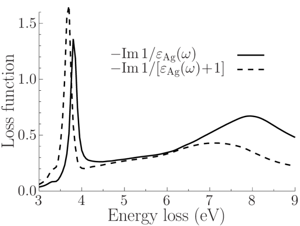
Figure 1: Bulk (solid line) and surface (dashed line) energy-loss functions of silver. The experimental optical dielectric function $\varepsilon_{\text{Ag}}(\omega)$ is used Palik (1985).

The purpose of this paper is, therefore, two-fold. First, we aim at the implementation of the theory of EELS of Ref. Nazarov, 1995 in its original form, i.e., that would treat the incident electron and the electrons of the target system on the same footing. Secondly, we apply this theory to the EELS of Ag surface, which is exactly the case when the interplay of the response of the target with the details of the probe’s motion is especially important, due to the overlap of the bulk and the surface features in the excitation spectrum of this material, as is illustrated in Fig. 1. Thereby we both further advance the theory of EELS and achieve an improvement in the understanding of the experimental spectra of the Ag surface.

Since the fully ab initio solution to the problem of the dielectric response of $d$-metals still remains a computationally formidable task, we have to resort to some model considerations. First, we substitute the three-dimensional (3D) problem with a one-dimensional (1D) one, neglecting the system’s non-uniformity in the surface plane. Second, the $d$-electrons are included in a phenomenological way, using the model of Liebsch Liebsch and Schaich (1995); Liebsch (1998) of the background DF. This work should, therefore, be considered as a step forward toward the full-featured 3D implementation of the same method, treating also $d$-electrons ab initio. However, the main ingredients of the theory (among them, importantly, the necessary inclusion of the optical potential) are presented and discussed in this work, facilitating the future implementation of the method in full.

The paper is organized as follows. In Sec. II we remind and further work out details of including the motion of the scattered electrons in the theory of EELS. In Sec. III, results of the calculations conducted with the use of our theory are presented and discussed. Conclusions are collected in Sec. IV. In the Appendix we detail on some important properties of the model utilized in the calculations. We use atomic units ($e^{2}=\hbar=m_{e}=1$) throughout unless otherwise indicated.

II Formalism

A formal solution to the problem of the inelastic scattering of an electron in the EELS setup, which incorporates the detailed quantum-mechanical motion of the projectile, can be quite generally written as Nazarov (1995); Nazarov and Nishigaki (2001)

$$\frac{d^{2}\sigma}{d\omega d\Omega}(\mathbf{p}^{\prime}\leftarrow\mathbf{p})=-\frac{16\pi^{3}p^{\prime}}{p}{\rm Im}\int\frac{\rho_{ext}^{*}(\mathbf{r}^{\prime\prime})}{|\mathbf{r}^{\prime\prime}-\mathbf{r}|}\chi(\mathbf{r},\mathbf{r}^{\prime},\omega)\frac{\rho_{ext}(\mathbf{r}^{\prime\prime\prime})}{|\mathbf{r}^{\prime}-\mathbf{r}^{\prime\prime\prime}|}d\mathbf{r}d\mathbf{r}^{\prime}d\mathbf{r}^{\prime\prime}d\mathbf{r}^{\prime\prime\prime},$$ (2)

where the left-hand side of Eq. (2) is the differential cross-section of the scattering from the state of the momentum $\mathbf{p}$ to a state of the momentum within the solid angle $d\Omega$ around $\mathbf{p}^{\prime}$, and to lose the energy within $d\omega$ around $\omega=(p^{2}-p^{\prime 2})/2$. In the right-hand side of Eq. (2), $\chi(\mathbf{r},\mathbf{r}^{\prime},\omega)$ is the interacting-electrons density-response function of the target, the complex-valued “external charge density”

$$\rho_{ext}(\mathbf{r})=\langle\mathbf{r}|\mathbf{p}^{+}\rangle^{*}\,\langle\mathbf{r}|{\mathbf{p}^{\prime}}^{-}\rangle,$$ (3)

is determined by the elastic scattering incoming and outgoing wave-functions, $|\mathbf{p}^{+}\rangle$ and $|\mathbf{p}^{-}\rangle$, respectively, which are the solutions to the Lippmann–Schwinger equation Taylor (1972)

$$\langle\mathbf{r}|\mathbf{p}^{\pm}\rangle=\langle\mathbf{r}|\mathbf{p}\rangle+G^{0}\!\left(\frac{p^{2}}{2}\pm\mathrm{i}0_{+}\right)V_{l}(\mathbf{r})\langle\mathbf{r}|\mathbf{p}^{\pm}\rangle,$$ (4)

where $G^{0}(E)$ is the non-interacting Green’s function, $V_{l}(\mathbf{r})$ is the single-particle static lattice potential, and $\langle\mathbf{r}|\mathbf{p}\rangle=e^{\mathrm{i}\mathbf{p}\cdot\mathbf{r}}/(2\pi)^{3/2}$ are plane-waves.

The structure of Eq. (2) has a transparent physical interpretation: The external charge $\rho_{ext}$ creates an external Coulomb potential, which, through the density-response function $\chi$, induces the charge fluctuation in the target. Finally, the Coulomb potential of that fluctuation couples to the external charge itself, causing the inelastic scattering of the latter.

It must be, however, emphasized that the above picture is no more than a convenient verbal description of the strict mathematical formalism presented in Ref. Nazarov, 1995: The derivation of Eq. (2) does not rely on the substitution of the true quantum-mechanical scattering problem for an electron with an artificial charge-density. It rather solves the problem of the combined elastic and inelastic scattering of a charge at an arbitrary many- (or a few) body system, which, with a mild assumption that the impinging electron can be considered distinguishable from those of the target, can be put into the terms of the density-response function of the target and the elastic scattering states of the projectile. Obtained within the distorted-wave approximationTaylor (1972), Eq. (2) is exact to the first order in the inelastic processes (the first Born approximation) and it is exact to all orders in the elastic scattering. It includes both the long- and the short-range interaction of the probe electron with the target, i.e., the dipole and impact scatteringLiebsch (1997), respectively, within, most importantly, the quantum-mechanical treatment of the probe itself.

Of course, practically, the quality of specific calculations by Eq. (2) depends on the accuracy of the approximations used to calculate its ingredients, i.e., the density-response function of the target $\chi$ and the wave-functions of the incoming and outgoing electron utilized in the construction of $\rho_{ext}$. We now turn to the use of specific models.

II.1 Model of a laterally uniform target

In this work we will use a simplification of the potential $V_{l}(\mathbf{r})$=$V_{l}(z)$ averaged in the plane parallel to the surface (which is chosen as the $xy$-plane, with the $z$-axis normal to the surface and directed into vacuum). In this case the wave-functions are plane-waves in the direction parallel to the surface

$$\langle\mathbf{r}|\mathbf{p}^{\pm}\rangle=\langle z|p_{z}^{\pm}\rangle\frac{e^{\mathrm{i}\mathbf{p}_{\|}\cdot\mathbf{r}_{\|}}}{2\pi},$$ (5)

where the subscript ‘parallel’ denotes the $xy$-projection of a vector. To take advantage of the scattering theory framework, in the following we represent the target with a sufficiently thick slab, with vacuum both above and below, which is also consistent with our numerical implementation of the method. Then $\langle z|p_{z}^{+}\rangle$ can be conveniently found as a solution to the Schrödinger equation with the following asymptotic boundary conditions

$$\langle z|p_{z}^{+}\rangle=\frac{1}{2\pi}\left\{\begin{array}[]{ll}a^{+}e^{\mathrm{i}p_{z}\,z}+b^{+}e^{-\mathrm{i}p_{z}\,z},&z\to+\infty,\\ c^{+}e^{\mathrm{i}p_{z}\,z}+d^{+}e^{-\mathrm{i}p_{z}\,z},&z\to-\infty,\end{array}\right.$$ (6)

$$\begin{split}&p_{z}>0:c^{+}=1,\ b^{+}=0,\\ &p_{z}<0:a^{+}=1,\ d^{+}=0.\end{split}$$ (7)

The asymptotic of $\langle z|p_{z}^{\prime-}\rangle$ is easily obtained from the relation

$$\langle z|p_{z}^{\prime-}\rangle=\langle z|-p_{z}^{\prime+}\rangle^{*}.$$ (8)

Therefore, using Eqs. (6) and (7), we have

$$\langle z|p_{z}^{\prime-}\rangle=\frac{1}{2\pi}\left\{\begin{array}[]{ll}a^{-}e^{\mathrm{i}p^{\prime}_{z}\,z}+b^{-}e^{-\mathrm{i}p^{\prime}_{z}\,z},&z\to+\infty,\\ c^{-}e^{\mathrm{i}p^{\prime}_{z}\,z}+d^{-}e^{-\mathrm{i}p^{\prime}_{z}\,z},&z\to-\infty,\end{array}\right.$$ (9)

$$\begin{split}&p^{\prime}_{z}>0:a^{-}=1,\ d^{-}=0,\\ &p^{\prime}_{z}<0:c^{-}=1,\ b^{-}=0.\end{split}$$ (10)

Equation (6) together with the lower line of Eq. (7) describes the electron incident on the surface, as in the low energy electron diffraction (LEED) experiment. Interestingly, the wave function of Eq. (9) together with the upper line of Eq. (10) is a time-reversed LEED state. This kind of function describes the photoelectron (PE) final state in the one-step theory of photoemission Fei (1974). Note that in vacuum it contains both outgoing and incoming beam. Thus, while in LEED and PE setups each of these kinds of the wave-functions enters separately, in EELS they are present together.

For $\rho_{ext}(\mathbf{r})$ we can write

$$\rho_{ext}(\mathbf{r})=\rho_{ext}(z)\frac{e^{\mathrm{i}\mathbf{q}_{\|}\cdot\mathbf{r}_{\|}}}{(2\pi)^{2}},$$ (11)

where

$$\rho_{ext}(z)=\langle z|p_{z}^{+}\rangle^{*}\langle z|p_{z}^{\prime-}\rangle,$$ (12)

and $\mathbf{q}_{\|}\!=\!\mathbf{p}_{\|}-\mathbf{p}_{\|}^{\prime}$. Then, finally, Eq. (2) takes the convenient form

$$\frac{1}{A}\frac{d^{2}\sigma}{d\omega d\Omega}(\mathbf{p}^{\prime}\leftarrow\mathbf{p})=-\frac{p^{\prime}}{\pi p\,q_{\|}^{2}}\,\text{Im}\int\rho_{ext}^{*}(z^{\prime\prime})e^{-q_{\|}|z^{\prime\prime}-z|}\chi(z,z^{\prime},q_{\|},\omega)e^{-q_{\|}|z^{\prime}-z^{\prime\prime\prime}|}\rho_{ext}(z^{\prime\prime\prime})dzdz^{\prime}dz^{\prime\prime}dz^{\prime\prime\prime},$$ (13)

where $A$ is the surface normalization area.

II.2 Real-space solution with the background dielectric function

According to Eq. (13), the external potential applied to our system is

$$\phi_{ext}(z)=\frac{2\pi}{q_{\|}}\int e^{-q_{\|}|z-z^{\prime}|}\rho_{ext}(z^{\prime})dz^{\prime}.$$ (14)

Therefore, Eq. (13) can be rewritten as

$$\frac{1}{A}\frac{d\sigma}{d\omega d\Omega}(\mathbf{p}^{\prime}\leftarrow\mathbf{p})\!=\!-\frac{p^{\prime}}{4\pi^{3}p}{\rm Im}\!\int\!\rho_{ext}^{*}(z^{\prime\prime})\phi_{ind}(z)dz,$$ (15)

where

$$\phi_{ind}(z)=\frac{2\pi}{q_{\|}}\int e^{-q_{\|}|z^{\prime}-z|}\chi(z^{\prime},z^{\prime\prime},q_{\|},\omega)\phi_{ext}(z^{\prime\prime})dz^{\prime}dz^{\prime\prime}$$ (16)

is the potential induced in the system in response to the external charge-density $\rho_{ext}(z)$. To determine $\phi_{ind}(z)$, a simplified model of Ag surface, introduced by Liebsch Liebsch and Schaich (1995); Liebsch (1998), is used, in which only $s$-electrons are treated quantum-mechanically through the calculation of their response function, while the influence of $d$-electrons is included effectively by the use of a background DF $\epsilon_{d}(\omega)$ comprising the half-space $z\leq b$, as schematized in Fig. 2.

Figure 2: Schematics of the model used in the calculation.

Then, for the total scalar potential $\phi(z)=\phi_{ext}(z)+\phi_{ind}(z)$ we can write separately in the regions I of $z\geq b$ and II of $z\leq b$

$$\phi(z)=\left\{\begin{array}[]{ll}\tilde{\phi}(z)+Ae^{-q_{\|}z},&z\geq b,\\ \dfrac{\tilde{\phi}(z)}{\epsilon_{d}}+Be^{q_{\|}z},&z\leq b,\end{array}\right.$$ (17)

where

$$\tilde{\phi}(z)=\phi_{ext}(z)+\phi_{s}(z),$$ (18)

$\phi_{s}(z)$ is the potential of the response of $s$-electrons only, and $A$ and $B$ are constants to be determined from the boundary conditions of the continuity of the tangential component of the electric field and the normal component of the electric displacement vector, which give, respectively,

$$\begin{split}&\tilde{\phi}(b)+Ae^{-q_{\|}b}=\frac{\tilde{\phi}(b)}{\epsilon_{d}}+Be^{q_{\|}b},\\ &-Ae^{-q_{\|}b}=Be^{q_{\|}b}\epsilon_{d}.\end{split}$$ (19)

For $\phi_{s}$ we can write

$$\begin{split}\phi_{s}(z)&=\frac{2\pi}{q_{\|}}\int e^{\ -q_{\|}|z-z^{\prime}|}\chi_{s}(z^{\prime},z^{\prime\prime},q_{\|},\omega)\\ &\times\left[\phi(z^{\prime\prime})-\phi_{s}(z^{\prime\prime})\right]dz^{\prime}dz^{\prime\prime},\end{split}$$ (20)

where $\chi_{s}$ is the density-response function of $s$-electrons only. By further rewriting Eq. (17) as

$$\begin{split}&\phi(z)-\phi_{s}(z)=\\ &\left\{\!\begin{array}[]{lll}\phi_{ext}(z)+Ae^{-q_{\|}z},&z\geq b,\\ \dfrac{\phi_{ext}(z)}{\epsilon_{d}}\!+\!\left(\dfrac{1}{\epsilon_{d}}\!-\!1\right)\phi_{s}(z)\!+\!Be^{q_{\|}z}&z\leq b,\end{array}\right.\end{split}$$ (21)

substituting Eq. (21) into the right-hand side of Eq. (20) and Eq. (18) into Eqs. (19), we arrive at a closed system of equations for $\phi_{s}(z)$, $A$, and $B$, which is numerically solved on a grid of $z$. Then from $\phi_{s}(z)$ we obtain $\tilde{\phi}(z)$ by Eq. (18), $\phi(z)$ by Eq. (17), and $\phi_{ind}(z)$ as $\phi(z)-\phi_{ext}(z)$. The latter is finally used in Eq. (15) to calculate the EEL spectrum.

III Calculations, results, and discussion

Our calculation of the ground-state of the $s$-electrons of the Ag (111) uses the 1D interpolation of the surface and the bulk potential of Ref. Chulkov et al., 1999. A super-cell with the period $d=221.7$ a.u. was used, which included 31 layers of the model $s$-subsystem of Ag, the rest occupied with vacuum. The time-dependent density-functional theory (TDDFT) calculation of the density-response function $\chi_{s}(z,z^{\prime},q_{\|},\omega)$ is performed on the level of the random-phase approximation (RPA), i.e., setting the exchange-correlation kernel Gross and Kohn (1985) $f_{xc}$ to zero. Then we apply the procedures of Secs. II.2 and II.1 to account for the response of $d$-electrons and to finally obtain the EEL spectra. The edge of the $d$-electrons was set at $b=0.717$ a.u. above the upper atomic layer. For $\varepsilon_{d}(\omega)$ we take

$$\varepsilon_{d}(\omega)=\varepsilon_{\text{Ag}}(\omega)-\left[\varepsilon_{s}(\omega)-1\right]=\varepsilon_{\text{Ag}}(\omega)+\frac{\omega_{p}^{2}}{\omega^{2}},$$ (22)

where $\varepsilon_{\text{Ag}}(\omega)$ is the experimental optical DF of silverPalik (1985) and $\varepsilon_{s}(\omega)=1-\omega_{p}^{2}/\omega^{2}$ is the Drude DF of $s$-electrons with the plasma frequency $\omega_{p}=9$ eV.

To construct $\rho_{ext}(z)$ by Eq. (12), we were solving the Schrödinger equation with the asymptotic boundary conditions of Eqs. (6) and (9). The scattering wave functions were obtained by solving the inverse band-structure problem as explained in Ref. Krasovskii and Schattke, 1997 and matching the Bloch solutions in the crystal to the linear combination of the incident and reflected wave in the vacuum. The same crystal potential as for the evaluation of $\chi$ was used, with the addition of the absorbing imaginary potential $-\mathrm{i}V_{\rm i}$ as explained below. Importantly, similar to the low-energy electron diffraction (LEED) theory Krasovskii et al. (2002), the inclusion of the optical potential (OP) into the Hamiltonian is necessary for EELS theory as well. This can be understood considering that, without OP, electrons having gone an arbitrarily long round-trip into the depth of the sample, would contribute to the spectrum. Since, in the first Born approximation, the probability of the bulk energy-loss is proportional to the path-length travelled, this would make the intensity of the bulk losses infinitely high. The influence of the deep interior of the sample is, however, suppressed, in LEED by all the inelastic processes, and in EELS by the inelastic processes beyond the first Born approximation. In the present calculation $V_{\rm i}$ was taken to be spatially constant in the solid and zero in vacuum. At $E_{p}=40$ eV it was $V_{\rm i}=0.3$ eV for the angle with the normal to the surface of $80^{\circ}$, $75^{\circ}$, $70^{\circ}$, $V_{\rm i}=0.5$ eV for $85^{\circ}$, and $V_{\rm i}=0.1$ eV for $55^{\circ}$. In Fig. 3 $\rho_{ext}(z)$ and the corresponding $\phi_{ext}(z)$ are shown for representative values of the parameters of the EELS experiment.

Figure 3: The complex-valued density of Eq. (12) (left panels) and the corresponding potential (right panels) as a function of the coordinate $z$ at $\omega=3.7$ eV, $\theta_{i}=80^{\circ}$, $\theta_{s}=75^{\circ}$, and $E_{p}=40$ eV. At these parameters, $q_{\|}=0.111$ a.u. The edge of the $d$-electrons is at $b=67.2$ a.u. and the period of the super-cell used in the calculation of the response of $s$-electrons is $d=221.7$ a.u. In the calculation, the origin is chosen in the center of the super-cell.

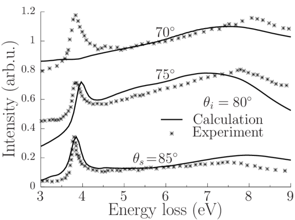
Figure 4: HREEL spectra of Ag (111) surface calculated within the framework of our theoretical approach (solid lines) compared to the experimental spectra of 10 monolayers of Ag on the Ni (111) surface, the latter compiled from Ref. Politano et al., 2013 (symbols). The energy of electrons in the incident beam is $E_{p}=40$ eV.

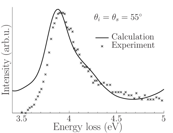
Figure 5: The same as Fig. 4, but for the specular reflection $\theta_{i}=\theta_{s}=55^{\circ}$.

In Figs. 4 and 5 results of calculations of the EEL reflection spectra are presented. They are compared to experimental HREELS of the system of 10 monolayers of Ag on (111) surface of Ni substrate Politano et al. (2013). In Fig. 4 the theoretical and experimental EEL spectra are shown for the primary energy of electrons $E_{p}=40$ eV, the angle of incidence $\theta_{i}=80^{\circ}$, and three values of the angle of scattering $\theta_{s}$ of $85^{\circ}$, $75^{\circ}$, and $70^{\circ}$. In Fig. 5 the results for the specular geometry with $\theta_{i}=\theta_{s}=55^{\circ}$ and the same primary energy are presented. The comparison of the theory with the experiment is reasonably good. Most importantly, the sharp bulk and surface plasmon peaks near 3.7 eV, separately present in the plots of the corresponding energy-loss functions (Fig. 1), are never resolved from each other in our calculations, but they form a joint broadened peak with a contribution from the both types of excitations. This is in full agreement with the HREELS experiments Rocca et al. (1995); Rocca (1995); Moresco et al. (1997); Politano et al. (2013). A notable exception from the agreement between the theory and the experiment is the case of $\theta_{i}=80^{\circ}$ and $\theta_{s}=70^{\circ}$, upper spectrum in Fig. 4, when, surprisingly, the lower-energy plasmon peak, which is strong in the experimental spectrum, is absent in the theoretical one.

To examine the latter discrepancy closer, in Fig. 6 we plot theoretical spectra for the angle of scattering gradually changing from $75^{\circ}$, when the peak in question is pronounced, to $70^{\circ}$, when this peak disappears. These results show that the strength of the peak near 3.7 eV decreases systematically when the scattering angle $\theta_{i}-\theta_{s}$ increases. We note that a similar effect of the disappearance of the 3.7 eV peak with the growing momentum can be observed in the results of the calculations of Ref. Silkin et al., 2015, performed in the dipole-scattering mode within the same model of $d$-electrons.

Figure 6: The calculated EEL spectra for the angle of scattering changing from $75^{\circ}$ to $70^{\circ}$ with the step of $1^{\circ}$. The gradual disappearance of the peak around 3.7 eV can be observed.

We analyze this tendency in detail in Appendix A to the conclusion that, although, the background DF model is applicable in the higher energy range around 8 eV to account for the bulk, surface, and the multipole plasmons in AgLiebsch and Schaich (1995); Liebsch (1998), it fails for the lower-energy plasmons at larger values of the wave-vector. Obviously, the future theory, which will include $d$-electrons from the first principles, will be free from this deficiency.

Since our calculations based on Eq. (2) are linear with respect to the interaction between the probe electron and the electronic subsystem of the target (distorted-waveTaylor (1972) with the first Born approximation for the inelastic processes), the multiple energy losses, e.g., multiple plasmon excitations, are beyond the capacity of this approach. Nonetheless, especially at higher primary energies, multiple losses can be expected in the experimental spectra. In Fig. 7 we plot the theoretical spectra together with the corresponding experimental ones for three different primary energies of 170, 100, and 70 eV at the specular geometry of $\theta_{i}=\theta_{s}=80^{\circ}$, where we now focus on the higher energy range. While the theoretical lines are rather smooth in this range, the experimental spectra at $E_{p}=$ 170 and 100 eV have prominent peaks around 7.6 eV. Considering that (i) the positions of these peaks are very close to the twice the energy of the strong single-plasmon peaks around 3.7 eV, (ii) their intensities change with $E_{p}$ consistently with those of the corresponding single-plasmon peaks, and (iii) these peaks are present in the experiment while absent in the linear-response based calculations, we are led to the conclusion that these peaks are due to the double-plasmon excitations.

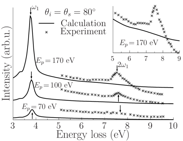
Figure 7: Primary energy dependence of HREELS of Ag (111). Peaks on the experimental spectra are attributed to the double-plasmon excitation and are, accordingly, absent at the theoretical spectra. The inset shows the same spectra for $E_{p}=170$ eV in a narrower energy range. The experimental data compiled from Ref. Politano et al., 2013 are used.

To reproduce the multiple plasmons theoretically, a theory of EELS beyond the first Born approximation is required. We note that the formal theory of inelastic scattering of a quantum-mechanical particle to the second Born approximation, expressed in terms of the quadratic density-response function of a target, was constructed in Ref. Nazarov and Nishigaki, 2002. The practical implementations of this theory have not, however, been yet developed.

IV Conclusions

We have revisited the problem of the energy losses by electrons in reflection electron energy-loss spectroscopy with the focus on the role of the probing electrons’ kinematics. The inadequacy of the description of EELS in terms of the energy-loss functions has been emphasized for the materials where the bulk and the surface features overlap or are close in energy in the excitation spectra. We have implemented the theory including the effect of the detailed quantum-mechanical motion of the probe electrons during their energy losses, using Ag surface as a representative example of a system where the kinematic aspect of the problem is particularly important.

Since our primary interest lies in the role of the kinematic effects, for a sophisticated problem of the $d$-electrons’ response we have used a simplified model of the background dielectric function, which has immensely simplified the numerical implementation. As a side effect, although we have found a reasonably good overall agreement with HREELS, at strongly off-specular geometries of the experiment, the theory and the measurements disagree. We have tracked this discrepancy down to the failure of the substitution of the $d$-electrons with the background dielectric function to describe the dispersion of the main loss feature of 3.7 eV in Ag at larger values of the momentum. Thus, the limits of the applicability of that, otherwise very useful model, have been set. This difficulty is anticipated to be overcome in the future theory, with all the ingredients included within the ab initio approach.

Another deviation of the theory from experiment we have found can be qualified as an evidence of the consistency of the former rather than its deficiency. Namely, the experiment shows peaks at EEL spectra that, by all the evidence, can be attributed to the double-plasmon excitations. The linear-response theory, which our approach is based on, fundamentally cannot account for such losses, and we do not, accordingly, obtain the double-excitation peaks in the calculations. Future implementations of the theory of the quadratic and higher-order response will be able to account for these processes.

Appendix A Properties of the model of the background DF

In this Appendix we scrutinize the model of the background DF used in this paper to account for the $d$-electrons in the dielectric response of silverLiebsch and Schaich (1995); Liebsch (1998). For the sake of maximal clarity, we do this analytically by considering the bulk response. In this case the same model is determined by the DF

$$\begin{split}\varepsilon(q,\omega)&=\varepsilon_{\text{Ag}}(\omega)-\left[1-\frac{\omega_{p}^{2}}{\omega^{2}}\right]+\varepsilon_{Ls}(q,\omega)\\ &=\varepsilon_{d}(\omega)+\left[\varepsilon_{Ls}(q,\omega)-1\right],\end{split}$$ (23)

where $\varepsilon_{\text{Ag}}(\omega)$ is the optical experimental DF of Ag, $\varepsilon_{d}(\omega)$ is given by Eq. (22), and $\varepsilon_{Ls}(q,\omega)$ is the Lindhard’s DF of the homogeneous electron gasLindhard (1954), taken at the density of the $s$-electrons of Ag.

Figure 8: The bulk energy-loss function using the DF of Eq. (23) plotted at several values of the wave-vector $q$. The plasmon peak near 3.7 eV clearly weakens and finally disappears with the increase of $q$.

In Fig. 8 we plot the energy-loss function with the use of the DF of Eq. (23) for several values of the wave-vector $q$. The plasmon peak near 3.7 eV weakens with the increase of $q$, until it disappears at $q\approx$ 0.2 a.u. This is consistent with the behavior of the DF itself plotted in Fig. 9. Indeed, for $q=$ 0 and 0.1 a.u., Re $\varepsilon(q,\omega)$ crosses zero in the corresponding energy range, thereby producing the plasmon peak in the loss-function. This is not the case any more for $q=$ 0.15, 0.175, and 0.2 a.u., although, for the former two wave-vectors, the peaks in question still persist in the loss-function due to the Re $\varepsilon$ approaching the zero axis (cf., Ref. Nazarov, 2015). Lastly, at $q=$ 0.2 a.u., Re $\varepsilon$ is very far from zero in this $\omega$-range, and no peak in the loss-function can be discerned any more.

Figure 9: The dielectric function of Eq. (23). Lines without labels are the real parts of the DF at the corresponding values of $q$. Lines with the label “Im” are imaginary parts, which, for all values of $q$, largely coincide with $-\text{Im}\,\varepsilon(q=0,\omega)$, since the Lindhard’s DF is real in the corresponding energy ranges.

The above results are consistent with those of Sec. III of this paper. Indeed, the main contribution to the $z$-component of the wave-vector of the external perturbation can be estimated from Eqs. (12), (6), and (9) as $p_{z}+p^{\prime}_{z}$ (note that $p_{z}<0$ and $p^{\prime}_{z}>0$). When $E_{p}=$ 40 eV and $\theta_{i}=$ 80^∘, this is equal to 0.123 and 0.259 a.u., for $\theta_{s}=$ 75^∘ and 70^∘, respectively. The corresponding values of $q_{\|}$ are 0.117 and 0.160 a.u., respectively. Then $q=[(p_{z}+p^{\prime}_{z})^{2}+q_{\|}^{2}]^{1/2}$ are 0.170 and 0.304 a.u., respectively, explaining the presence of the plasmon near 3.7 eV in the theoretical spectra in the former and its absence in the latter case. For the specular geometry in Fig. 5, the corresponding value is $q=$ 0.09 a.u., consistent with the strong theoretical lower-energy plasmon peak in this figure. The same argument holds for the spectra in Fig. 7.

Experimentally, however, this prediction of the model is not supported, as can be seen in Fig. 4, upper experimental spectrum: the plasmon near 3.7 eV persists in the measurements on Ag at larger wave-vectors. We, therefore, can conclude that, at larger wave-vectors, the response of $d$-electrons cannot be realistically substituted with a wave-vector independent dielectric function, when it concerns the lower-energy plasmon in Ag, while this model is quite successful in the higher energy range, where the spectra are dominated by the response of $s$-electrons outside the $d$-electrons backgroundLiebsch and Schaich (1995); Liebsch (1998).

References

- Hillier and Baker (1944) J. Hillier and R. F. Baker, “Microanalysis by means of electrons,” Journal of Applied Physics 15, 663–675 (1944).
- Ibach and Mills (1982) H. Ibach and D. L. Mills, Electron Energy Loss Spectroscopy and Surface Vibrations (Academic Press, New York, 1982).
- Eberlein et al. (2008) T. Eberlein, U. Bangert, R. R. Nair, R. Jones, M. Gass, A. L. Bleloch, K. S. Novoselov, A. Geim, and P. R. Briddon, “Plasmon spectroscopy of free-standing graphene films,” Phys. Rev. B 77, 233406 (2008).
- Egerton (2009) R. F. Egerton, “Electron energy-loss spectroscopy in the TEM,” Reports on Progress in Physics 72, 016502 (2009).
- Pines and Nozieres (1966) D. Pines and P. Nozieres, The theory of quantum liquids (Benjamin, New York, 1966).
- Ritchie (1957) R. H. Ritchie, “Plasma losses by fast electrons in thin films,” Phys. Rev. 106, 874–881 (1957).
- Bennett (1970) A. J. Bennett, “Influence of the electron charge distribution on surface-plasmon dispersion,” Phys. Rev. B 1, 203–207 (1970).
- Tsuei et al. (1990) K.-D. Tsuei, E. W. Plummer, A. Liebsch, K. Kempa, and P. Bakshi, “Multipole plasmon modes at a metal surface,” Phys. Rev. Lett. 64, 44–47 (1990).
- Liebsch (1998) A. Liebsch, “Prediction of a Ag multipole surface plasmon,” Phys. Rev. B 57, 3803–3806 (1998).
- Liebsch (1997) A. Liebsch, Electronic excitations at metal surfaces (Plenum, New-York, 1997).
- Nazarov (2015) V. U. Nazarov, “Electronic excitations in quasi-2D crystals: what theoretical quantities are relevant to experiment?” New Journal of Physics 17, 073018 (2015).
- Nazarov (1995) V. U. Nazarov, “Analytical properties of dielectric response of semi-infinite systems and the surface electron energy loss function,” Surface Science 331–333, 1157 – 1162 (1995).
- Taylor (1972) J. R. Taylor, Scattering theory (John Wiley & Sons, New York, 1972).
- Kohn and Sham (1965) W. Kohn and L. J. Sham, “Self-consistent equations including exchange and correlation effects,” Phys. Rev. 140, A1133–A1138 (1965).
- Nazarov (1999) V. U. Nazarov, “Multipole surface-plasmon-excitation enhancement in metals,” Phys. Rev. B 59, 9866–9869 (1999).
- Nazarov and Nishigaki (2001) V. U. Nazarov and S. Nishigaki, “Inelastic low energy electron diffraction at metal surfaces,” Surface Science 482 - 485, 640 – 647 (2001).
- Politano et al. (2013) A. Politano, V. Formoso, and G. Chiarello, “Collective electronic excitations in thin Ag films on Ni(111),” Plasmonics 8, 1683–1690 (2013).
- Palik (1985) Edward D. Palik, ed., Handbook of Optical Constants of Solids (Academic Press, New York, 1985).
- Liebsch and Schaich (1995) A. Liebsch and W. L. Schaich, “Influence of a polarizable medium on the nonlocal optical response of a metal surface,” Phys. Rev. B 52, 14219–14234 (1995).
- Note (1) In contrast to the Kohn-Sham , includes electron-electron interactions, and the two response functions are related as , where is the xc kernel Gross and Kohn (1985).
- Note (2) In Refs. \rev@citealpnumNazarov-95S,Nazarov-01 the solution was given in the momentum space, of which Eq. (2) is the Fourrier transform.
- Fei (1974) “Photoemission spectroscopy–Correspondence between quantum theory and experimental phenomenology,” Phys. Rev. B 10, 4932–4947 (1974).
- Chulkov et al. (1999) E. V. Chulkov, V. M. Silkin, and P. M. Echenique, “Image potential states on metal surfaces: binding energies and wave functions,” Surface Science 437, 330 – 352 (1999).
- Gross and Kohn (1985) E. K. U. Gross and W. Kohn, “Local density-functional theory of frequency-dependent linear response,” Phys. Rev. Lett. 55, 2850–2852 (1985).
- Krasovskii and Schattke (1997) E. E. Krasovskii and W. Schattke, “Surface electronic structure with the linear methods of band theory,” Phys. Rev. B 56, 12874–12883 (1997).
- Krasovskii et al. (2002) E. E. Krasovskii, W. Schattke, V. N. Strocov, and R. Claessen, “Unoccupied band structure of by very low-energy electron diffraction: Experiment and theory,” Phys. Rev. B 66, 235403 (2002).
- Rocca et al. (1995) M. Rocca, L. Yibing, F. Buatier de Mongeot, and U. Valbusa, “Surface plasmon dispersion and damping on Ag(111),” Phys. Rev. B 52, 14947–14953 (1995).
- Rocca (1995) M. Rocca, “Low-energy {EELS} investigation of surface electronic excitations on metals,” Surface Science Reports 22, 1 – 71 (1995).
- Moresco et al. (1997) F. Moresco, M. Rocca, V. Zielasek, T. Hildebrandt, and M. Henzler, “ELS-LEED study of electronic excitations on Ag(110) and Ag(111),” Surface Science 388, 24 – 32 (1997).
- Silkin et al. (2015) V. M. Silkin, P. Lazić, N. Došlić, H. Petek, and B. Gumhalter, “Ultrafast electronic response of Ag(111) and Cu(111) surfaces: From early excitonic transients to saturated image potential,” Phys. Rev. B 92, 155405 (2015).
- Nazarov and Nishigaki (2002) V. U. Nazarov and S. Nishigaki, “-order theory of quantum inelastic scattering of charges by solids,” Phys. Rev. B 65, 094303 (2002).
- Lindhard (1954) J. Lindhard, “On the properties of a gas of charged particles,” K. Dan. Vidensk. Selsk. Mat.-Fys. Medd. 28, 1 (1954).