∎
Tel.: +86-471-4994853
Fax: +86-471-4991650
55email: mathliuyang@aliyun.com 66institutetext: J.F. Wang 77institutetext: School of Statistics and Mathematics, Inner Mongolia University of Finance and Economics, Hohhot, 010070, China
A two-grid finite element approximation for a nonlinear time-fractional Cable equation
Abstract
In this article, a nonlinear fractional Cable equation is solved by a two-grid algorithm combined with finite element (FE) method. A temporal second-order fully discrete two-grid FE scheme, in which the spatial direction is approximated by two-grid FE method and the integer and fractional derivatives in time are discretized by second-order two-step backward difference method and second-order weighted and shifted Grünwald difference (WSGD) scheme, is presented to solve nonlinear fractional Cable equation. The studied algorithm in this paper mainly covers two steps: First, the numerical solution of nonlinear FE scheme on the coarse grid is solved; Second, based on the solution of initial iteration on the coarse grid, the linearized FE system on the fine grid is solved by using Newton iteration. Here, the stability based on fully discrete two-grid method is derived. Moreover, the a priori estimates with second-order convergence rate in time is proved in detail, which is higher than the L1-approximation result with . Finally, the numerical results by using the two-grid method and FE method are calculated, respectively, and the CPU-time is compared to verify our theoretical results.
Keywords:
Two-grid method WSGD operator Nonlinear time-fractional Cable equation Finite element method Error results1 Introduction
Fractional partial differential equations (FPDEs), which have a lot of applications in the realm of science, mainly include space FPDEs Wanghyd ; Me2 ; Sousa2 ; Huangcm1 ; Xiaoa1 ; Xuqw1 ; Roop , time FPDEs Baleanu5 ; Caojx2 ; Dinghf1 ; Xucj1 ; Heyn1 ; Sunhw1 ; Atangana2 ; Mclean1 ; Chencm4 ; Lukashchuk ; Sunzzwuxn and space-time FPDEs Qianqian1 ; Liufw2 ; El-Wakil . The construction of numerical methods for FPDEs has attracted great attention of many scholars. For example, finite element (FE) methods have been successfully applied to solving many FPDEs in the current literatures. In Roop , Roop gave FE method for fractional advection dispersion equations on bounded domains in two-dimensions. In Liufw2 , Feng et al. studied FE method for diffusion equation with space-time fractional derivatives. In MA1 , Ma et al. used moving FE methods to solve space fractional differential equations. Li et al. in Ljc2 gave some numerical theories on FE methods for Maxwell’s equations. In Liuyli Liu et al. proposed a mixed FE method for a fourth-order time-FPDE with first-order convergence rate in time. In Liuylh2 , Liu et al. solved a time-fractional reaction-diffusion problem with fourth-order space derivative term by using FE method and L1-approximation. In Jinbt6 Jin et al. used a FE method to solve the space-fractional parabolic equation, and gave the error analysis. In Zengfh1 Zeng et al. used FE approaches combined with finite difference method for solving the time fractional subdiffusion equation. In Ford Ford et al. studied a FE method for time FPDEs and obtained optimal convergence error estimates. Bu et al. Tang1 discussed Galerkin FE method for Riesz space fractional diffusion equations in two-dimensional case. In LCP1 , Li et al. applied FE method to solving nonlinear fractional subdiffusion and superdiffusion equations. In Dengwh7 , Deng solved fractional Fokker-Planck equation with space and time derivatives by using FE method. In Wu1 , Zhang et al. implemented FE method for solving a modified fractional diffusion equation in two-dimensional case.
In this article, we will consider a two-grid FE algorithm for solving a nonlinear time-fractional Cable equation
| (1) |
which covers boundary condition
| (2) |
and initial condition
| (3) |
where is a bounded convex polygonal sub-domain of , whose boundary is continuous. is the time interval with the upper bound . The source item and the initial function are given known functions. For the nonlinear term , there exists a constant such that and . And is Riemann-Liouville fractional derivative with given in Definition 1.
The fractional Cable equation Henry ; Bisquert ; Henry1 ; Tomovski1 , which reflects the anomalous electro-diffusion in nerve cells, is an important mathematical model. For the fractional Cable equation, we can find some numerical methods, such as finite difference methods Chencm1 ; Zhanglm1 ; Yubo ; Yusteq ; QQ , orthogonal spline collocation method Zhanghx1 , spectral approximations Bhrawy1 ; Xucj6 , finite element methods Zhuangph1 ; Liuylh . Chen et al. Chencm1 , Hu and Zhang Zhanglm1 , Yu and Jiang Yubo , Quintana-Murillo and Yuste Yusteq , presented and analyzed some finite difference schemes to numerically solve the fractional cable equation from different perspectives. Liu et al. QQ , solved numerically the fractional cable equation by using two implicit numerical schemes. Zhang et al. Zhanghx1 proposed and analyzed the discrete-time orthogonal spline collocation method for the two-dimensional case of fractional cable equation. Bhrawy and Zaky Bhrawy1 presented a Jacobi spectral collocation approximation for numerically solving nonlinear two-dimensional fractional cable equation covering Caputo fractional derivative. Lin et al. Xucj6 developed spectral approximations combined with finite difference method for looking for the numerical solution of the fractional Cable equation. Recently, Zhuang et al. Zhuangph1 , Liu et al. Liuylh studied and analyzed Galerkin finite element methods for the fractional Cable equation with Riemann-Liouville derivative, respectively, and did some different analysis based on different approximate formula for fractional derivative. Here, we will consider a two-grid FE algorithm combined with a higher-order time approximation to seek the numerical solutions of nonlinear fractional Cable equation.
Two-grid FE algorithm was presented and developed by Xu Xuj1 ; Xuj2 . Owing to holding the advantage of saving computation time, many computational scholars have used well the method to numerically solve integer-order partial differential equations(such as Dawson and WheelerDawson for nonlinear parabolic equations; Zhong et al. zhonglq for for time-harmonic Maxwell equations; Mu and Xu Xuj4 for mixed Stokes-Darcy model; Chen and Chen Cheny3 for nonlinear reaction-diffusion equations; Bajpai and Nataraj Baj for Kelvin-Voigt model; Wang Wangws1 for semilinear evolution equations with positive memory) and developed some new numerical techniques based on the idea of two-grid algorithm (two-grid expanded Mixed FE methods in Chen et al. Cheny1 , Wu and Allen Wul1 , Liu et al. Ruih3 ; two-grid finite volume element method in Chen and Liu Ruih2 ). Until recently, in Liuylh1 , the two-grid FE method was presented to solve the nonlinear fourth-order fractional differential equations with Caputo fractional derivative. However, the Caputo time fractional derivative was approximated by L1-formula and the only ()-order convergence rate in time was arrived at in Liuylh1 .
In this article, our main task is to look for the numerical solution of nonlinear fractional Cable equation (1) with initial and boundary condition by using two-grid FE method with higher-order time approximate scheme Dengwhtw ; Vongwang1 and to discuss the numerical theories on stability and a priori estimate analysis for this method. In Dengwhtw , Tian et al. approximated the Riemann-Liouville fractional derivative by proposing a new higher-order WSGD operator, then discussed some finite difference scheme based on this operator. Considering this idea of WSGD operator, Wang and Vong Vongwang1 presented the compact difference scheme for the modified anomalous sub-diffusion equation with -order Caputo fractional derivative, in which the Caputo fractional derivative covering order is approximated by applying the idea of WSGD operator, and an extension for this idea was also made to discuss a compact difference scheme for the fractional diffusion-wave equation. However, the theories of the FE methods based on the idea of WSGD operator have not been studied and discussed. Especially, the two-grid FE algorithm combined with the idea of the WSGD operator has not been reported in the current literatures. Here, we will study the two-grid FE scheme with WSGD operator for solving nonlinear fractional Cable equation, derive the stability of the studied method, and prove a priori estimate results with second-order convergence rate, which is higher than time convergence rate obtained by usual L1-approximation. Finally, we do some numerical computations by using the current method and standard nonlinear FE method, respectively, and find that our method in CPU-time is more efficient than standard nonlinear FE method.
Throughout this article, we will denote as a constant, which is free of the spatial coarse grid size , fine step length , and time mesh size . Further, we define the natural inner product in or by equipped with norm .
The remaining outline of the article is as follows. In section 2, some definitions of fractional derivatives, lemmas on time approximations and two-grid algorithm combined with second-order scheme in time are given. In section 3, the analysis of stability of two-grid FE method is made. In section 4, a priori errors of two-grid FE algorithm are proved. In section 5, some numerical results by using two-grid FE method and standard nonlinear FE method are computed and some comparisons of computing time are done. Finally, some remarking conclusions on two-grid FE algorithm proposed in this paper are shown in section 6.
2 Fractional derivatives and two-grid FE method
2.1 Fractional derivatives and approximate formula
In many literatures, we can get the following definitions on fractional derivatives of Caputo type and Riemann-Liouville type. At the same time, we need to give some useful lemmas in the subsequent theoretical analysis.
Definition 1
The -order fractional derivative of Riemann-Liouville type for the function is defined as
| (4) |
Definition 2
The -order fractional derivative of Caputo type for the function is defined by
| (5) |
where is Gamma function.
Lemma 1
Sunzzjc The relationship between Caputo fractional derivative and Riemann-Liouville fractional derivative can be given by
| (6) |
Lemma 2
Lemma 3
For series defined in lemma 2, we have
| (10) |
Lemma 4
For series given by (8), the following inequality holds for any integer
| (11) |
Proof. Noting that the notation (8), we have
| (12) |
Applying triangle inequality and lemma 3, we arrive at
| (13) |
So, we get the conclusion of lemma.
Lemma 5
Remark 1
Based on the relationship (6) between Caputo fractional derivative and Riemann-Liouville fractional derivative, we easily find that the equality with holds. Further, it is not hard to know that the second-order discrete formula (7) in lemma 2 can also approximate the Caputo fractional derivative (5) with zero initial value.
2.2 Two-grid algorithm based on FE scheme
To give the fully discrete analysis, we should approximate both integer and fractional derivatives. The grid points in the time interval are labeled as , , where is the time step length. We define for a smooth function on and .
Using the approximate formula (7) and two-step backward Euler approximation, then applying Green’s formula, we find to arrive at the weak formulation of (1)-(3) for any as
Case :
| (15) |
Case :
| (16) |
where
| (17) |
| (18) |
| (19) |
For formulating finite element algorithm, we choose finite element space as
| (20) |
where is the quasiuniform rectangular partition for the spatial domain .
Then, we find to formulate a standard nonlinear finite element system for any as
Case :
| (21) |
Case :
| (22) |
For improving the finite element discrete system (21)-(22), we consider the following two-grid FE system based on the coarse grid and the fine grid .
Step I: First, the following nonlinear system based on the coarse grid is solved by finding the solution such that
Case :
| (23) |
Case :
| (24) |
Step II: Second, based on the solution on the coarse grid , the following linear system on the fine grid , is considered by looking for such that
Case :
| (25) |
Case :
| (26) |
where .
Remark 2
In the solving system above, we can seek a solution on the coarse grid in the nonlinear system (23)-(LABEL:3.33), then get the solution on the fine grid in the linear system (25)-(LABEL:3.35). We call the system (23)-(LABEL:3.33) with (25)-(LABEL:3.35) as two-grid FE system, which is more efficient than the standard nonlinear FE system (21)-(22). In the results of numerical calculations, we will see the CUP-time used by two-grid FE scheme is less than that by standard nonlinear FE scheme.
In what follows, for the convenience of discussions on stability and a priori error analysis, we first give the following lemma.
Lemma 6
For series , the following inequality holds
| (27) |
where
| (28) |
3 Analysis of stability based on two-grid FE algorithm
We first derive the stability based on two-grid FE algorithm.
Theorem 1
For the two-grid FE system (23)-(LABEL:3.35) based on coarse grid and fine grid , the following stable inequality for holds
| (29) |
Proof. We first consider the results for the case . Setting in (LABEL:3.35), and noting that the inequality (27), we have
| (30) |
Using Cauchy-Schwarz inequality and Young inequality, we easily get
| (31) |
Sum (LABEL:3.81) for from to and use (27) to get
| (32) |
Set in (25) and use Cauchy-Schwarz inequality and Young inequality to arrive at
| (33) |
From (LABEL:3.83), it easily follows that
| (34) |
Make a combination for (LABEL:3.82) and (LABEL:3.85) to get
| (35) |
Note that lemma 5 and use Cronwall lemma to get
| (36) |
For the next estimates, we have to discuss the term .
4 Error analysis based on two-grid algorithm
For discussing and deriving a priori error estimates based on fully discrete two-grid FE method, we have to introduce a Ritz-projection operator which is defined by finding such that
| (39) |
with the following estimate
| (40) |
where is coarse grid step length or fine grid size and the norms are defined by with the polynomial’s degree .
In the following contents, based on the given Ritz-projection 14 and estimate inequality (40), we will do some detailed discussions on a priori error analysis.
Now we rewrite the errors as
Theorem 2
With , and , we obtain the following a priori error results in -norm
| (41) |
where is a positive constant independent of coarse grid step length , fine grid size and time step parameters .
Proof. Combine (LABEL:3.35) and (7) with (39) to arrive at the error equations for any and
| (42) |
In what follows, we need to estimate the terms . First we estimate the third term . For considering the nonlinear term, we use Taylor expansion to obtain
| (43) |
where is a value between and .
Based on (43), we obtain
| (44) |
So, we have
| (45) |
We now use Cauchy-Schwarz inequality with Young inequality to get
| (46) |
and
| (47) |
By using lemma 4 with Cauchy-Schwarz inequality and Young inequality, we have
| (48) |
In (LABEL:5.31), (LABEL:3.14)-(48), we take and make a combination for these expressions to get
| (49) |
Multiply (LABEL:7.1) by and sum (LABEL:7.1) for from to to get
| (50) |
Subtract (25) from (15), we have
| (51) |
In (LABEL:3.39), we choose and use (LABEL:3.14) and (48) to get
| (52) |
Simplifying for (LABEL:3.42) and using triangle inequality, we have
| (53) |
Combine (LABEL:4.25) with (LABEL:3.40) and note that to get
| (54) |
By using the Cronwall lemma and the relationship (22), we have for sufficiently small
| (55) |
For the next discussion, we need to give the estimate for the term .
Subtract (23), (LABEL:3.33) from (15), (16), respectively and use the Ritz-projection (39)
to arrive at the error equations under the coarse grid for any
Case :
| (56) |
Case :
| (57) |
where , .
In (LABEL:5.30) and (LABEL:5.3), we take and , respectively, and use a similar process of proof to the estimate for to get
| (58) |
Substitute the above estimate inequality (58) into (55)
| (59) |
which combine the triangle inequality with (40) to get the conclusion of theorem 2.
Remark 3
Based on the theorem’s results, we obtain the temporal convergence rate with second-order result, which is free of fractional parameters and . Moreover, we can find that the time convergence rate by using second-order backward difference method and second-order WSGD scheme is higher than the one with obtained by L1-approximation.
5 Numerical Tests
In this section, we consider a numerical example in space-time domain to verify the theoretical results of two-grid FE algorithm combined with second-order backward difference method and second-order WSGD scheme. We now choose the nonlinear term and the exact solution , then easily determine that the known source function in (1) is
We now divide uniformly the spatial domain by using rectangular meshes, approximate first-order integer derivative with two-step backward Euler method and discretize the fractional direvative with second-order scheme. Now we take the continuous bilinear functions space with .
For showing the current method in the this paper, we calculate some error results with convergence order for different fractional parameters and . In Table 1, by taking fractional parameters , and fixed temperal step length , we show some a priori errors in -norm and convergence orders for two-grid algorithm with coarse and fine meshes and FE method with . From Table 1, ones can see that the results with second-order convergence rate by using our method is stable and the CPU-time in seconds for two-grid FE method is less than that by making use of the standard FE method. In Table 2, we use the same computing method and spatial meshes as in Table 1, then obtain the errors and convergence rates when taking , and . The similar calculated results with , and are also shown in Table 3. These numerical results shown in Tables 1-3 also tell ones that compared to widely used L1-formula with , the WSGD scheme in this paper can get second-order convergence rate. For obtaining the second-order accuracy in time, we here use the second-order backward difference method to approximate time direction. Compared to commonly used one-step backward Euler difference method, for getting the same calculated accuracy, the second-order backward difference method can reduce the number of iterations in time and save the calculating time. From the numerical results presented in Tables 1-2, ones can see that the convergence order of our method is slightly higher than that of the standard nonlinear FE method, while in Table 3, our method shows the similar convergence rate to that of nonlinear FE method. These phenomena indicate that compared to nonlinear FE method, our method has advantages in solving the time fractional Cable equation covering the space-time partial derivative term with larger fractional parameter .
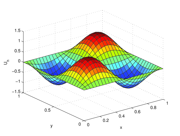
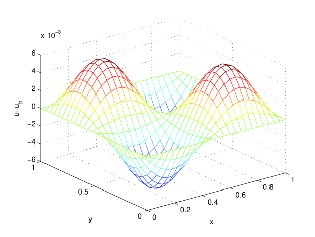
In Figures 1-3, by taking , , and , we show the surfaces for the exact solution , two-grid FE solution and FE solution , respectively. Ones easily see that both two-grid FE solution based on coarse and fine meshes and FE solution can approximate well the exact solution . Especially, from the surface for errors and in Figures 4-5, ones easily find that two-grid FE method holds the similar computational accuracy to that of standard nonlinear FE method.
In summary, from the computed error results and convergence rate in Tables 1-3 and the surfaces shown in Figures 1-5, ones can know that with the similar computational accuracy to that for standard nonlinear FE method, our two-grid FE method is more efficient in computational time than the standard nonlinear FE method. Moreover, the current method combined with the second-order backward difference method and second-order WSGD operater can get a stable second-order convergence rate, which is independent of fractional parameters and and is higher than the convergence result derived by L1-approximation.
6 Some concluding remarks
In this article, we consider two-grid method combined with FE methods to give the numerical solution for nonlinear fractional Cable equations. First, we give some lemmas used in our paper; Second, we give the approximate formula for fractional derivative, then formulate the numerical scheme based on two-grid FE method; Finally, we do some detailed derivations for the stability of numerical scheme and a priori error analysis with second-order convergence rate in time, then compute some numerical errors and convergence orders to verify the theoretical results.
From the numerical results, ones easily see that two-grid FE method studied in this paper can solve well the nonlinear time fractional Cable equation. Based on the point of view of calculating efficiency, compared to FE method, two-grid FE method can spend less time. Moreover, compared with the time convergence rate obtained by usual L1-approximation, the current numerical scheme can arrive at second-order convergence rate independent of fractional parameters and . Considering the mentioned advantages, in the future works, we will discuss the numerical theories of two-grid FE method for some space and space-time fractional partial differential equations with nonlinear term.
Acknowledgements
Authors thank the anonymous referees and editors very much for their valuable comments and suggestions, which greatly help us improve this work. This work is supported by supported by the National Natural Science Fund (11301258, 11361035), Natural Science Fund of Inner Mongolia Autonomous Region (2015MS0114), and the Postgraduate Scientific Research Innovation Foundation of Inner Mongolia (No. 1402020201337).


| Order | CPU time (in seconds) | |||
|---|---|---|---|---|
| 1/4 | 1/16 | 6.3566e-003 | - | 43.231369 |
| 1/5 | 1/25 | 2.6118e-003 | 1.9930 | 122.612277 |
| 1/6 | 1/36 | 1.2323e-003 | 2.0600 | 414.219975 |
| 1/7 | 1/49 | 6.3532e-004 | 2.1489 | 1810.428349 |
| FE algorithm | Order | CPU time (in seconds) | ||
| 1/16 | 6.4246e-003 | - | 49.760083 | |
| 1/25 | 2.6815e-003 | 1.9578 | 145.938800 | |
| 1/36 | 1.3025e-003 | 1.9803 | 488.617402 | |
| 1/49 | 7.0575e-004 | 1.9876 | 2112.565940 |
| Order | CPU time (in seconds) | |||
|---|---|---|---|---|
| 1/4 | 1/16 | 6.6252e-003 | - | 34.637650 |
| 1/5 | 1/25 | 2.7694e-003 | 1.9545 | 102.802120 |
| 1/6 | 1/36 | 1.3488e-003 | 1.9729 | 374.852060 |
| 1/7 | 1/49 | 7.3406e-004 | 1.9733 | 1745.224030 |
| FE algorithm | Order | CPU time (in seconds) | ||
| 1/16 | 6.6292e-003 | - | 37.660242 | |
| 1/25 | 2.7735e-003 | 1.9525 | 116.171144 | |
| 1/36 | 1.3529e-003 | 1.9687 | 448.280514 | |
| 1/49 | 7.3816e-004 | 1.9651 | 2189.299786 |
| Order | CPU time (in seconds) | |||
|---|---|---|---|---|
| 1/4 | 1/16 | 6.9107e-003 | - | 53.860030 |
| 1/5 | 1/25 | 2.8841e-003 | 1.9581 | 153.053853 |
| 1/6 | 1/36 | 1.4003e-003 | 1.9815 | 497.518498 |
| 1/7 | 1/49 | 7.5807e-004 | 1.9905 | 2040.087416 |
| FE algorithm | Order | CPU time(in seconds) | ||
| 1/16 | 6.9107e-003 | - | 57.108134 | |
| 1/25 | 2.8841e-003 | 1.9581 | 163.841391 | |
| 1/36 | 1.4003e-003 | 1.9815 | 554.982539 | |
| 1/49 | 7.5809e-004 | 1.9904 | 2416.876270 |
References
- (1) Wang, H., Yang, D.P., Zhu, S.F.: Inhomogeneous Dirichlet boundary-value problems of space-fractional diffusion equations and their finite element approximations. SIAM J. Numer. Anal. 52(3) (2014) 1292-1310.
- (2) Meerschaert, M.M., Tadjeran, C.: Finite difference approximations for two-sided space-fractional partial differential equations. Appl. Math. Comput. 56(1), 80-90 (2006)
- (3) Sousa, E.: An explicit high order method for fractional advection diffusion equations. J. Comput. Phys. 278, 257-274 (2014)
- (4) Wang, P.D., Huang, C.M.: An energy conservative difference scheme for the nonlinear fractional Schrödinger equations. J. Comput. Phys. 293, 238-251 (2015)
- (5) Ding, Z., Xiao, A., Li, M.: Weighted finite difference methods for a class of space fractional partial differential equations with variable coefficients. J. Comput. Appl. Math. 233(8), 1905-1914 (2010)
- (6) Xu, Q.W., Hesthaven, J.S.: Discontinuous Galerkin method for fractional convection-diffusion equations. SIAM J. Numer. Anal. 52(1), 405-423 (2014)
- (7) Roop, J.P.: Computational aspects of FEM approximation of fractional advection dispersion equations on bounded domains in . J. Comput. Appl. Math. 193(1), 243-268 (2006)
- (8) Jafari, H., Kadkhoda, N. Baleanu, D.: Fractional Lie group method of the time-fractional Boussinesq equation, Nonlinear Dyn. 81, 1569-1574 (2015)
- (9) Cao, J.X., Li, C.P., Chen, Y.Q.: Compact difference method for solving the fractional reaction-subdiffusion equation with Neumann boundary value condition. Int. J. Comput. Math. 92(1), 167-180 (2015)
- (10) Ding, H.F., Li, C.P.: High-order compact difference schemes for the modified anomalous subdiffusion equation. arXiv 1408.5591 (2014)
- (11) Lin, Y.M., Xu, C.J.: Finite difference/spectral approximations for the time-fractional diffusion equation. J. Comput. Phys. 225(2), 1533-1552 (2007)
- (12) Wei, L.L., He, Y.N.: Analysis of a fully discrete local discontinuous Galerkin method for time-fractional fourth-order problems. Appl. Math. Model. 38(4), 1511-1522 (2014)
- (13) Gao, G.H., Sun, H.W.: Three-point combined compact difference schemes for time-fractional advection-diffusion equations with smooth solutions. J. Comput. Phys. 298, 520-538 (2015)
- (14) Atangana, A., Baleanu, D.: Numerical solution of a kind of fractional parabolic equations via two difference schemes. Abstr. Appl. Anal. 2013, 8 (2013) Article ID 828764.
- (15) Mustapha, K., McLean, W.: Superconvergence of a discontinuous Galerkin method for fractional diffusion and wave equations. SIAM J. Numer. Anal. 51, 491-515 (2013)
- (16) Chen, C., Liu, F., Turner, I., Anh, V.: A Fourier method for the fractional diffusion equation describing sub-diffusion. J. Comput. Phys. 227, 886-897 (2007)
- (17) Lukashchuk, S.Y.: Conservation laws for time-fractional subdiffusion and diffusion-wave equations. Nonlinear Dyn. 80(1-2), 791-802 (2015)
- (18) Sun, Z.Z., Wu, X.N.: A fully discrete difference scheme for a diffusion-wave system. Appl. Numer. Math. 56(2), 193-209 (2006)
- (19) Yang, Q., Turner, I., Liu, F., Ilic, M.: Novel numerical methods for solving the time-space fractional diffusion equation in two dimensions. SIAM J. Sci. Comput. 33(3), 1159-1180 (2011)
- (20) Feng, L.B., Zhuang, P., Liu, F., Turner, I., Gu, Y.T.: Finite element method for space-time fractional diffusion equation. Numer. Algorithms, 10.1007/s11075-015-0065-8 (2015)
- (21) El-Wakil, S.A., Abulwafa, E.M.: Formulation and solution of space-time fractional Boussinesq equation. Nonlinear Dyn. 80(1-2), 167-175 (2015)
- (22) Ma, J.T., Liu, J.Q., Zhou, Z.Q.: Convergence analysis of moving finite element methods for space fractional differential equations. J. Comput. Appl. Math. 255, 661-670 (2014)
- (23) Li, J.C., Huang, Y.Q., Lin, Y.P.: Developing finite element methods for maxwell’s equations in a cole-cole dispersive medium. SIAM J. Sci. Comput. 33(6), 3153-3174 (2011)
- (24) Liu, Y., Fang, Z.C., Li, H., He, S.: A mixed finite element method for a time-fractional fourth-order partial differential equation. Appl. Math. Comput. 243, 703-717 (2014)
- (25) Liu, Y., Du, Y.W., Li, H., He, S., Gao, W.: Finite difference/finite element method for a nonlinear time-fractional fourth-order reaction-diffusion problem. Comput. Math. Appl. 70(4), 573-591 (2015)
- (26) Jin, B.T., Lazarov, R., Pasciak, J., Zhou, Z.: Error analysis of a finite element method for the space-fractional parabolic equation. SIAM J. Numer. Anal. 52(5), 2272-2294 (2014)
- (27) Zeng, F., Li, C., Liu, F., Turner, I.: The use of finite difference/element approaches for solving the time fractional subdiffusion equation. SIAM J. Sci. Comput. 35(6), A2976-A3000 (2013)
- (28) Ford, N.J., Xiao, J.Y., Yan, Y.B.: A finite element method for time fractional partial differential equations. Fract. Calc. Appl. Anal. 14(3), 454-474 (2011)
- (29) Bu, W.P., Tang, Y.F., Yang, J.Y.: Galerkin finite element method for two-dimensional Riesz space fractional diffusion equations. J. Comput. Phys. 276, 26-38 (2014).
- (30) Li, C.P., Zhao, Z.G., Chen, Y.Q.: Numerical approximation of nonlinear fractional differential equations with subdiffusion and superdiffusion. Comput. Math. Appl. 62(3), 855-875 (2011)
- (31) Deng, W.H.: Finite element method for the space and time fractional Fokker-Planck equation. SIAM J. Numer. Anal. 47(1), 204-226 (2008)
- (32) Zhang, N., Deng, W.H., Wu, Y.J.: Finite difference/element method for a two-dimensional modified fractional diffusion equation. Adv. Appl. Math. Mech. 4, 496-518 (2012)
- (33) Henry, B., Langlands, T.A.M.: Fractional cable models for spiny neuronal dendrites. Phys. Rev. Lett. 100, 128103 (2008)
- (34) Bisquert J.: Fractional diffusion in the multipletrapping regime and revision of the equivalence with the continuous-time random walk. Phys. Rev. Lett. 91(1), 010602(4) (2003)
- (35) Langlands, T.A.M., Henry, B., Wearne, S.: Fractional cable equation models for anomalous electrodiffusion in nerve cells: infinite domain solutions. J. Math. Biol. 59(6), 761-808 (2009)
- (36) Saxena, R.K., Tomovski, Z., Sandev, T.: Analytical solution of generalized space-time fractional Cable equation. Mathematics, 3, 153-170 (2015)
- (37) Chen, C.M., Liu, F., Burrage, K.: Numerical analysis for a variable-order nonlinear Cable equation. J. Comput. Appl. Math. 236(2), 209-224 (2011)
- (38) Hu, X.L. Zhang, L.M.: Implicit compact difference schemes for the fractional cable equation. Appl. Math. Model. 36, 4027-4043 (2012)
- (39) Yu, B. Jiang, X.Y.: Numerical identification of the fractional derivatives in the two-dimensional fractional Cable equation. J. Sci. Comput. DOI 10.1007/s10915-015-0136-y.
- (40) Quintana-Murillo, J., Yuste, S.B.: An explicit numerical method for the fractional Cable equation. Int. J. Differ. Equ. 2011, Article ID 231920, (2011)
- (41) Liu, F., Yang, Q., Turner, I.: Two new implicit numerical methods for the fractional Cable equation. J. Comput. Nonlinear Dyn. 6(1), 011009 (2011)
- (42) Zhang, H.X., Yang, X.H., Han, X.L.: Discrete-time orthogonal spline collocation method with application to two-dimensional fractional Cable equation. Comput. Math. Appl. 68, 1710-1722 (2014)
- (43) Bhrawy, A.H. Zaky, M.A.: Numerical simulation for two-dimensional variable-order fractional nonlinear cable equation. Nonlinear Dyn. 80(1-2), 101-116 (2015)
- (44) Lin, Y.M., Li, X.J., Xu, C.J.: Finite difference/spectral approximations for the fractional Cable equation. Math. Comput. 80, 1369-1396 (2011)
- (45) Zhuang, P., Liu, F., Turner, I., Anh, V.: Galerkin finite element method and error analysis for the fractional cable equation. Numer. Algor. DOI 10.1007/s11075-015-0055-x.
- (46) Liu, J.C., Li, H., Liu, Y.: A new fully discrete finite difference/element approximation for fractional Cable equation. J. Appl. Math. Comput. DOI 10.1007/s12190-015-0944-0.
- (47) Xu, J.C.: A novel two-grid method for semilinear elliptic equations. SIAM J. Sci. Comput. 15, 231-237 (1994)
- (48) Xu, J.C.: Two-grid discretization techniques for linear and nonlinear PDEs. SIAM J. Numer. Anal. 33, 1759-1777 (1996)
- (49) Dawson, C.N., Wheeler, M.F.: Two-grid methods for mixed finite element approximations of nonlinear parabolic equations. Contemp. Math. 180, 191-203 (1994)
- (50) Zhong, L.Q., Shu, S., Wang, J., Xu, J.: Two-grid methods for time-harmonic Maxwell equations. Numer. Linear Algebra Appl. 20(1), 93-111 (2013)
- (51) Mu, M., Xu, J.C.: A two-grid method of a mixed Stokes-Darcy model for coupling fluid flow with porous media flow. SIAM J. Numer. Anal. 45(5), 1801-1813 (2007)
- (52) Chen, L., Chen, Y.P.: Two-grid method for nonlinear reaction-diffusion equations by mixed finite element methods. J. Sci. Comput. 49, 383-401 (2011)
- (53) Bajpai, S., Nataraj, N.: On a two-grid finite element scheme combined with Crank-Nicolson method for the equations of motion arising in the Kelvin-Voigt model. Comput. Math. Appl. 68(12, Part B), 2277-2291 (2014)
- (54) Wang, W.S.: Long-time behavior of the two-grid finite element method for fully discrete semilinear evolution equations with positive memory. J. Comput. Appl. Math. 250, 161-174 (2013)
- (55) Chen, Y.P., Huang, Y.Q., Yu, D.H.: A two-grid method for expanded mixed finite-element solution of semilinear reaction-diffusion equations. Int. J. Numer. Meth. Eng. 57(2), 193-209 (2003)
- (56) Wu, L., Allen, M.B.: A two grid method for mixed finite element solution of reaction-diffusion equations. Numer. Methods Partial Differ. Equ. 15, 317-332 (1999).
- (57) Liu, W., Rui, H.X., Hu, F.Z.: A two-grid algorithm for expanded mixed finite element approximations of semi-linear elliptic equations. Comput. Math. Appl. 66, 392-402 (2013)
- (58) Chen, C., Liu, W.: A two-grid method for finite volume element approximations of second-order nonlinear hyperbolic equations. J. Comput. Appl. Math. 233, 2975-2984 (2010)
- (59) Liu, Y., Du, Y.W., Li, H., Li, J.C., He, S.: A two-grid mixed finite element method for a nonlinear fourth-order reaction-diffusion problem with time-fractional derivative. Comput. Math. Appl. 70(10), 2474-2492 (2015)
- (60) Tian, W.Y., Zhou, H., Deng, W.H.: A class of second order difference approximations for solving space fractional diffusion equations. Math. Comput. 84, 1703-1727 (2015)
- (61) Wang, Z.B., Vong, S.W.: Compact difference schemes for the modified anomalous fractional sub-diffusion equation and the fractional diffusion-wave equation. J. Comput. Phys. 277, 1-15 (2014)
- (62) Ji, C.C., Sun, Z.Z.: A high-order compact finite difference scheme for the fractional sub-diffusion equation. J. Sci. Comput. 64(3), 959-985 (2015)
- (63) Ciarlet, P.G.: The Finite Element Method for Elliptic Problems. North-Holland, Amsterdam, The Netherlands, (1978)