Abstract

The Raney numbers $R_{p,r}(k)$ are a two-parameter generalization of the Catalan numbers. In this paper, we obtain a recurrence relation for the Raney numbers which is a generalization of the recurrence relation for the Catalan numbers. Using this recurrence relation, we confirm a conjecture posed by Amdeberhan concerning the enumeration of $(s,s+1)$-core partitions $\lambda$ with parts that are multiples of $p$. We then give a new combinatorial interpretation for the Raney numbers $R_{p+1,r+1}(k)$ with $0\leq r<p$ in terms of $(kp+r,kp+r+1)$-core partitions $\lambda$ with parts that are multiples of $p$.

Keywords: Raney number, Catalan number, core partition, hook length, poset, order ideal, coral diagram

AMS Subject Classifications: 05A15, 05A17, 06A07

1 Introduction

In this paper, we build a connection between the Raney numbers and $(s,s+1)$-core partitions with parts that are multiples of $p$. We show that the number of $(kp+r,kp+r+1)$-core partitions with parts that are multiples of $p$ equals the Raney number $R_{p+1,r+1}(k)$, confirming a conjecture posed by Amdeberhan [1].

The Raney numbers were introduced by Raney in his investigation of functional composition patterns [13] and these numbers have also been used in probability theory [11, 12]. The Raney numbers are defined as follows:

$$R_{p,r}(k)=\frac{r}{kp+r}{kp+r\choose k}.$$ (1.1)

The Raney numbers are a two-parameter generalization of the Catalan numbers. To be more specific, if $r=1$, the Raney numbers specialize to the Fuss-Catalan numbers $C_{p}(k)$ [8, 9], where $C_{p}(k)$ are the numbers of $k$-ary trees with labeled $p$ vertices and

$$C_{p}(k)=R_{p,1}(k)=\frac{1}{(p-1)k+1}{kp\choose k}.$$

If we further set $p=2$, we obtain the usual Catalan numbers $C_{k}$, that is,

$$R_{2,1}(k)=C_{k}=\frac{1}{k+1}{2k\choose k}.$$ (1.2)

In [9], Hilton and Pedersen obtained the following relation for the Raney numbers $R_{p,r}(k)$ and the Fuss-Catalan numbers $C_{p}(k)$.

Theorem 1.1

Let p be a positive integer and let $r,k$ be nonnegative integers. Then we have

$$R_{p,r}(k)=\sum_{i_{1}+\ldots+i_{r}=k}C_{p}(i_{1})C_{p}(i_{2})\ldots C_{p}(i_{r}).$$

Based on Theorem 1.1, Beagley and Drube [5] gave a combinatorial interpretation for the Raney numbers in terms of coral diagrams which we will describe in Section 2.

Let us give an overview of notation and terminology on partitions. A partition $\lambda$ of a positive integer $n$ is a finite nonincreasing sequence of positive integers $(\lambda_{1},\lambda_{2},\ldots,\lambda_{m})$ such that $\lambda_{1}+\lambda_{2}+\cdots+\lambda_{m}=n$. We write $\lambda=(\lambda_{1},\lambda_{2},\ldots,\lambda_{m})\vdash n$ and we say that $n$ is the size of $\lambda$ and $m$ is the length of $\lambda$. The Young diagram of $\lambda$ is defined to be an up- and left-justified array of $n$ boxes with $\lambda_{i}$ boxes in the $i$-th row. Each box $B$ in $\lambda$ determines a hook consisting of the box $B$ itself and boxes directly to the right and directly below $B$. The hook length of $B$, denoted $h(B)$, is the number of boxes in the hook of $B$.

For a partition $\lambda$, the $\beta$-set of $\lambda$, denoted $\beta(\lambda)$, is defined to be the set of hook lengths of the boxes in the first column of $\lambda$. For example, Figure 1 illustrates the Young diagram and the hook lengths of a partition $\lambda=(5,3,2,2,1)$. The $\beta$-set of $\lambda$ is $\beta(\lambda)=\{9,6,4,3,1\}$. Notice that a partition $\lambda$ is uniquely determined by its $\beta$-set. Given a decreasing sequence of positive integers $(h_{1},h_{2},\ldots,h_{m})$, it is easily seen that the unique partition $\lambda$ with $\beta(\lambda)=\{h_{1},h_{2},\ldots,h_{m}\}$ is

$$\lambda=(h_{1}-(m-1),h_{2}-(m-2),\dots,h_{m-1}-1,h_{m}).$$ (1.3)

9& 7 4 21

6 4 1

4 2

3 1

1

Figure 1: The Young diagram of $\lambda=(5,3,2,2,1)$

For a positive integer $t$, a partition $\lambda$ is a $t$-core partition, or simply a $t$-core, if it contains no box whose hook length is a multiple of $t$. Let $s$ be a positive integer not equal to $t$, we say that $\lambda$ is an $(s,t)$-core if it is simultaneously an $s$-core and a $t$-core. For example, the partition $\lambda=(5,3,2,2,1)$ in Figure 1 is a $(5,8)$-core.

Let $s$ and $t$ be two coprime positive integers. Anderson [3] showed that the number of $(s,t)$-core partitions equals ${s+t\choose s}/(s+t)$. It specializes to the Catalan number $C_{s}=\frac{1}{s+1}{2s\choose s}$ if $t=s+1$. Ford, Mai and Sze [7] proved that the number of self-conjugate $(s,t)$-core partitions equals ${\lfloor\frac{s}{2}\rfloor+\lfloor\frac{t}{2}\rfloor\choose\lfloor\frac{s}{2}\rfloor}$. Furthermore, Olsson and Stanton [14] proved that there exists a unique $(s,t)$-core partition with the maximum size $(s^{2}-1)(t^{2}-1)/24$. A simpler proof was provided by Tripathi [17]. More results on $(s,t)$-core partitions can be found in [2, 4, 6, 10, 16, 18, 19].

In [1], Amdeberhan posed the following conjecture.

Conjecture 1.1

Let $s$ and $p$ be positive integers. The number of $(s,s+1)$-core partitions $\lambda$ with parts that are multiples of $p$ equals

$$\frac{s+1-p\lfloor\frac{s}{p}\rfloor}{s+1}{s+\lfloor\frac{s}{p}\rfloor\choose s}.$$ (1.4)

We observe that the expression (1.4) appearing in Conjecture 1.1 equals the Raney number $R_{p+1,r+1}(k)$ if we write $s=kp+r$, where $0\leq r<p$. To prove conjecture 1.1, in Section $2$, we shall deduce a recurrence relation for the Raney numbers by using coral diagrams. In Section $3$, we shall give a characterization of the $\beta$-set of the conjugate of an $(s,s+1)$-core partition with parts that are multiples of $p$. Based on this characterization, we show that the number of $(kp+r,kp+r+1)$-core partitions with parts that are multiples of $p$ have the same recurrence relation with the Raney number $R_{p+1,r+1}(k)$. This proves Conjecture 1.1.

2 Raney numbers

In this section, we investigate the Raney numbers by using coral diagrams. We obtain a recurrence relation for the Raney numbers which is a generalization of the recurrence relation for the Catalan numbers. We begin by introducing some graph theoretic terminology.

Let $p$ be a positive integer. Then a p-star is a rooted tree with $p$ terminal edges lying above a single base vertex. A coral diagram of type $(p,r,k)$ is a rooted tree which is constructed from an $r$-star via the repeated placement of k $p$-stars atop terminal edges. Let $D(p,r,k)$ denote the set of coral diagrams of type $(p,r,k)$. We can construct a coral diagram $D\in D(p,r,k)$ by attaching $p$-stars one “tier” at a time. We begin with the base tree and work upward. Figure 2 illustrates a coral diagram of type $(2,3,3)$.

Figure 2: Construction of a coral diagram of type $(2,3,3)$

We note that the definition of coral diagrams differs slightly from the one defined by Beagley and Drube [5]. In [5], a coral diagram of type $(p,r,k)$ is a rooted tree which is constructed from an $(r+1)$-star via the repeated placement of k $p$-stars atop terminal edges that are not the leftmost edge adjacent to the root. Not attaching $p$-stars to the leftmost edge adjacent to the root gives them a consistent way of selecting a base vertex for planar embedding. Anyhow, the coral diagrams under the two definitions have the same enumeration.

We need the following theorem due to Beagley and Drube [5].

Theorem 2.1

Let $p$ be a positive integer and let $r,k$ be nonnegative integers. Then the number of coral diagrams of type $(p,r,k)$ equals the Raney number $R_{p,r}(k)$, that is,

$$|D(p,r,k)|=R_{p,r}(k).$$

Using Theorem 2.1, we obtain recurrence relations for Raney numbers, as follows.

Theorem 2.2

Let $p$ be a positive integer and let $r,k$ be nonnegative integers. Then we have

$$R_{p,1}(k)= \sum_{i=0}^{k-1}R_{p,1}(i)R_{p,p-1}(k-1-i),$$ (2.1)

$$R_{p,r}(k)= \sum_{i=0}^{k}R_{p,1}(i)R_{p,r-1}(k-i),r>1.$$ (2.2)

And the Raney numbers $R_{p,r}(k)$ are uniquely determined by the above relations together with initial values $R_{p,r}(0)=1$, $R_{p,0}(k+1)=0$.

Proof.  The initial values $R_{p,r}(0)=1$, $R_{p,0}(k+1)=0$ follow directly from the expression (1.1) for the Raney numbers, that is,

$$R_{p,r}(k)=\frac{r}{kp+r}{kp+r\choose k}.$$

Now we assume that $k>0$, $r>0$. From Theorem 2.1, we see that $R_{p,r}(k)$ equals the number of coral diagrams of type $(p,r,k)$, that is,

$$R_{p,r}(k)=|D(p,r,k)|.$$

We proceed to investigate the recurrence relations for Raney numbers $R_{p,r}(k)$ by using coral diagrams. Let $D$ be a coral diagram in $D(p,r,k)$. There are two cases.

If $r>1$, we divide the coral diagram $D$ into two coral diagrams $D_{1}$ and $D_{2}$ by splitting the root of $D$ such that the root of the coral diagram $D_{1}$ is only adjacent to the leftmost edge and the root of the coral diagram $D_{2}$ is adjacent to the rest $r-1$ edges. See Figure 3 as an example. Assume that the coral diagram $D_{1}$ has $i$ $p$-stars, then the coral diagram $D_{2}$ has $k-i$ $p$-stars. It yields that $D_{1}\in D(p,1,i)$ which is counted by $R_{p,1}(i)$, and $D_{2}\in D(p,r-1,k-i)$ which is counted by $R_{p,r-1}(k-i)$. Since the coral diagram $D$ is uniquely determined by $D_{1}$ and $D_{2}$, we obtain the relation (2.2), that is,

$$R_{p,r}(k)=\sum_{i=0}^{k}R_{p,1}(i)R_{p,r-1}(k-i).$$

If $r=1$, then $D$ is constructed from a 1-star. Contracting the edge of this 1-star into a new vertex, we obtain a new coral diagram $D^{\prime}$. It is easily seen that $D^{\prime}$ is a coral diagram in $D(p,p,k-1)$, which is counted by $R_{p,p}(k-1)$. Hence we have $R_{p,1}(k)=R_{p,p}(k-1)$. If further $p=1$, since $R_{1,0}(k)=0$ when $k>0$, relation (2.1) is equivalent to $R_{1,1}(k)=R_{1,1}(k-1)$. By the expression (1.1) for the Raney numbers $R_{p,r}(k)$, it can be easily checked that $R_{1,1}(k)=R_{1,1}(k-1)=1$. Hence relation (2.1) holds if $r=p=1$. Now assume that $p>1$. Combining relation (2.2) and $R_{p,1}(k)=R_{p,p}(k-1)$, we obtain (2.1).

To prove that the Raney numbers are uniquely determined by the relations (2.1) and (2.2) together with initial values $R_{p,r}(0)=1$, $R_{p,0}(k+1)=0$, we use induction on $k$. If $k=0$, we have that $R_{p,r}(0)=1$. Suppose we can determine all the values of the Raney numbers $R_{p,r}(k)$ with $k\leq n$ from the relations (2.1) and (2.2) together with initial values. We proceed to show that $R_{p,r}(n+1)$ can be determined. First, $R_{p,1}(n+1)$ can be determined by (2.1). Then by (2.2), the values of $R_{p,2}(n+1),R_{p,3}(n+1),R_{p,4}(n+1)\cdots$ can be obtained in turn. Thus we can determine all the values of the Raney numbers $R_{p,k}(n+1)$. By induction, all the Raney numbers $R_{p,r}(k)$ can be determined. This completes the proof.  

From (1.2), we have that $C_{k}=R_{2,1}(k)$. Substituting $p=2$ into (2.1), we obtain the recurrence relation for the Catalan numbers $C_{k}=\sum_{i=0}^{k-1}C_{i}C_{k-1-i}$.

Figure 3: Dividing a coral diagram into two coral diagrams

3 Proof of Conjecture 1.1

In this section, we shall give a characterization of the $\beta$-set of the conjugate of an $(s,s+1)$-core partition with parts that are multiples of $p$. Using this characterization, we prove Conjecture 1.1 posed by Amdeberhan. We then give a new combinatorial interpretation for the Raney numbers $R_{p+1,r+1}(k)$ with $0\leq r<p$ in terms of $(kp+r,kp+r+1)$-core partitions $\lambda$ with parts that are multiples of $p$.

We observe that the expression (1.4) appearing in Conjecture 1.1 equals the Raney number $R_{p+1,r+1}(k)$ if we write $s=kp+r$, where $0\leq r<p$. That is,

$$\frac{s+1-p\lfloor\frac{s}{p}\rfloor}{s+1}{s+\lfloor\frac{s}{p}\rfloor\choose s}=\frac{kp+r+1-kp}{kp+r+1}{kp+r+k\choose kp+r}$$

$$=\frac{r+1}{k(p+1)+r+1}{k(p+1)+r+1\choose k}=R_{p+1,r+1}(k).$$

Hence Conjecture 1.1 can be restated as the following equivalent theorem.

Theorem 3.1

Let $s$ and $p$ be positive integers. Suppose that $s=kp+r$, where $0\leq r<p$. Then the number of $(s,s+1)$-core partitions $\lambda$ with parts that are multiples of $p$ equals the Raney number $R_{p+1,r+1}(k)$.

To prove the above theorem, we shall give a characterization of the $\beta$-set $\beta(\lambda^{c})$, where $\lambda^{c}$ is the conjugate of an $(s,s+1)$-core partition $\lambda$ with parts that are multiples of $p$. Let us recall some notation and terminology on posets.

Let $P$ be a poset. For two elements $x$ and $y$ in $P$, we say $y$ covers $x$ if $x<y$ and there exists no element $z\in P$ satisfying $x<z<y$. The Hasse diagram of a finite poset $P$ is a graph whose vertices are the elements of $P$, whose edges are the cover relations, and such that if $y$ covers $x$ then there is an edge connecting $x$ and $y$ and $y$ is placed above $x$. An order ideal of $P$ is a subset $I$ such that if any $y\in I$ and $x\leq y$ in $P$, then $x\in I$. Let $J(P)$ denote the set of order ideals of $P$. For more details on poset, see Stanley [15].

In the following lemma, Anderson [3] established a correspondence between core partitions and order ideals of a certain poset by mapping a partition to its $\beta$-set.

Lemma 3.2

Let $s,t$ be two coprime positive integers, and let $\lambda$ be a partition of $n$. Then $\lambda$ is an $(s,t)$-core partition if and only if $\beta(\lambda)$ is an order ideal of $P_{(s,t)}$. where

$$P_{(s,t)}=\mathbb{N}^{+}\setminus\{n\in\mathbb{N}^{+}\mid n=k_{1}s+k_{2}t\mbox{ for some }k_{1},k_{2}\in\mathbb{N}\}$$

and $y$ covers $x$ in $P_{(s,t)}$ if $y-x\in\{s,t\}$.

For example, let $s=3$ and $t=4$. We can construct all $(3,4)$-core partitions by finding order ideals of $P_{(3,4)}$. It is easily checked that $P_{(3,4)}=\{1,2,5\}$ with the partial order $5>2$ and $5>1$. Hence the order ideals of $P_{(3,4)}$ are $\emptyset$, $\{1\}$, $\{2\}$, $\{2,1\}$ and $\{5,2,1\}$. The corresponding $(3,4)$-core partitions are $\emptyset$, $(1)$, $(2)$, $(1,1)$ and $(3,1,1)$, respectively. Let $T_{s}=P_{(s,s+1)}$. From Lemma 3.2, the Hasse diagram of $T_{s}$ can be easily constructed. For example, Figure 4 illustrates the Hasse diagram of the poset $T_{6}$.

Figure 4: The Hasse diagram of $T_{6}$

Let $\lambda$ be an $(s,s+1)$-core partition with parts that are multiples of $p$ and let $\lambda^{c}$ be the conjugate of $\lambda$. Since $\lambda^{c}$ is also an $(s,s+1)$-core partition, from Lemma 3.2, we see that $\beta(\lambda^{c})$ is an order ideal in $T_{s}$. The following lemma gives a further description of $\beta(\lambda^{c})$.

Lemma 3.3

Let $\lambda$ be a partition with parts that are multiples of $p$ and let $\lambda^{c}$ be the conjugate of $\lambda$. Then the length of each maximal consecutive integers in $\beta(\lambda^{c})$ is divided by $p$.

Proof.  Suppose that $\lambda^{c}=(a_{1}^{m_{1}},a_{2}^{m_{2}},\ldots a_{n}^{m_{n}})$, where $a_{1}>a_{2}>\cdots>a_{n}$ and $a_{i}^{m_{i}}$ means $m_{i}$ occurrences of $a_{i}$. Since $\lambda$ is a partition with parts that are multiples of $p$, we have that $m_{i}(1\leq i\leq n)$ is a multiple of $p$. Then the lemma follows directly from the relation of a partition and its $\beta$-set shown in (1.3).  

Let $S$ be an integer set and let $l$ be a positive integer. We say that the set $S$ has property $P_{l}$ if the length of each maximal consecutive integers in $S$ is divided by $l$. For example, the integer set $\{1,2,3,6,7,8,9,10,11\}$ has property $P_{3}$.

Let $\lambda$ be a partition. From Lemma 3.2 and Lemma 3.3, we see that $\lambda$ is an $(s,s+1)$-core partition with parts that are multiple of $p$ if and only if $\beta(\lambda^{c})$ is an order ideal in $T_{s}$ with property $P_{p}$. Let $s$ and $p$ be positive integers. Suppose that $s=kp+r$, where $0\leq r<p$. Let $C_{p,r}(k)$ denote the number of order ideals in $T_{s}$ with property $P_{p}$. We set $C_{p,-1}(k)=0$ if $k>0$ and $p\geq 0$. Hence to prove Theorem 3.1, it suffices to show that $C_{p,r}(k)=R_{p+1,r+1}(k)$.

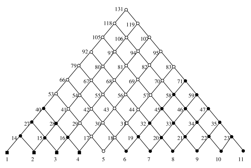
We proceed to compute the number of order ideals in $T_{s}$ with property $P_{p}$. To this end, we shall partition $J(T_{s})$ according to the smallest missing element of rank $0$ in an order ideal. Note that the elements of rank $0$ in $T_{s}$ are just the minimal elements. For $1\leq i\leq s-1$, let $J_{i}(T_{s})$ denote the set of order ideals of $T_{s}$ such that $i$ is the smallest missing element of rank $0$. Let $J_{s}(T_{s})$ denote the set of order ideals which contain all minimal elements in $T_{s}$. Then we can write $J(T_{s})$ as

$$J(T_{s})=\bigcup_{i=1}^{s}J_{i}(T_{s}).$$

Figure 5 gives an illustration of the elements contained in an order ideal in $J_{5}(T_{12})$. We see that an order ideal $I\in J_{5}(T_{12})$ must contain the elements labeled by squares, but does not contain any elements represented by open circles. The elements represented by solid circles may or may not appear in $I$. That is, $I$ can be decomposed into three parts, one is $\{1,2,3,4\}$, one is isomorphic to an order ideal of $T_{4}$ and one is isomorphic to an order ideal of $T_{7}$.

Figure 5: The elements of an order ideal $I\in J_{5}(T_{12})$

In general, for $1\leq i\leq s$ and an order ideal $I\in J_{i}(T_{s})$, we can decompose it into three parts: one is $\{1,2,\ldots,i-1\}$, one is isomorphic to an order ideal of $T_{i-1}$ and one is isomorphic to an order ideal of $T_{s-i}$ (Some parts may be empty). We shall use this decomposition to prove Theorem 3.1.

Proof of Theorem 3.1. We prove this theorem by showing that $C_{p,r}(k)$ and $R_{p+1,r+1}(k)$ have the same recurrence relation and initial values. If $k=0$, that is, $s=r<p$. Then the unique order ideal in $T_{r}$ with property $P_{p}$ is $\emptyset$. By the definition of $C_{p,r}(k)$, we have that $C_{p,r}(0)=1=R_{p+1,r+1}(0)$. Combining with $C_{p-1,-1}(k)=R_{p,0}(k)=0$, where $k>0$, we see that $C_{p,r}(k)$ have the same initial values with $R_{p+1,r+1}(k)$.

We proceed to show that $C_{p,r}(k)$ and $R_{p+1,r+1}(k)$ have the same recurrence relation. Suppose now $k\geq 1$. Let $I$ be an order ideal in $J(T_{s})$ with property $P_{p}$. Then $I\in J_{ip+1}(T_{s})$, where $0\leq i\leq\lfloor\frac{s-1}{p}\rfloor$ since $I$ has property $P_{p}$. $I$ can be decomposed into three parts: one is $\{1,2,\ldots,ip\}$, one is isomorphic to an order ideal $I_{1}$ of $T_{ip}$ and one is isomorphic to an order ideal $I_{2}$ of $T_{s-1-ip}$. Since the absolute difference of any two numbers in two parts are larger than $1$, we have that all of the three parts $\{1,2,\ldots,ip\}$, $I_{1}$ and $I_{2}$ have property $P_{p}$.

It is easily seen that the number of order ideals in $T_{ip}$ with property $P_{p}$ is counted by $C_{p,0}(i)$. To enumerate the number of order ideals in $T_{s-1-ip}$ with property $P_{p}$, we consider two cases. If $r=0$, namely $s=kp$, then $s-1-ip=(k-i-1)p+(p-1)$. It follows that the number of order ideals in $T_{s-1-ip}$ with property $P_{p}$ is counted by $C_{p,p-1}(k-i-1)$. If $r>0$, then $s-1-ip=(k-i)p+r-1$. So in this case, the number of order ideals in $T_{s-1-ip}$ with property $P_{p}$ is counted by $C_{p,r-1}(k-i)$.

Combining the two cases, we have that

$$C_{p,0}(k)= \sum_{i=0}^{k-1}C_{p,0}(i)C_{p,p-1}(k-i-1),$$

$$C_{p,r}(k)= \sum_{i=0}^{k}C_{p,0}(i)C_{p,r-1}(k-i),r>0.$$

It can be checked that $C_{p,r}(k)$ have the same recurrence relation with the Raney numbers $R_{p+1,r+1}(k)$ as shown in Theorem 2.2. By a similar discussion as in the proof of Theorem 2.2, we obtain that $C_{p,r}(k)$ are uniquely determined by the above relations together with the initial values. Hence we have that $C_{p,r}(k)=R_{p+1,r+1}(k)$. This completes the proof.  

From Theorem 3.1, we see that the Raney numbers $R_{p+1,r+1}(k)$ with $0\leq r<p$ equal the numbers of $(kp+r,kp+r+1)$-core partitions with parts that are multiples of $p$. This gives a new combinatorial interpretation for these Raney numbers.

Acknowledgments. This work was supported by the National Science Foundation of China.

References

- [1] T. Amdeberhan, Theorems, problems and conjectures, arXiv:1207.4045.
- [2] T. Amdeberhan and E. Leven, Multi-cores, posets, and lattice paths, arXiv:1406.2250.
- [3] J. Anderson, Partitions which are simultaneously - and -core, Discrete Math., 248 (2002), 237–243.
- [4] D. Armstrong, C.R.H. Hanusa and B.C. Jones, Results and conjectures on simultaneous core partitions, European J. Combin., 41 (2014), 205–220.
- [5] J.E. Beagley, P. Drube, The Raney genralization of Catalan numbers and the enumeration of planar embeddings, Australasian J. Combin., 63 (2015). 130–141.
- [6] W.Y.C. Chen, H.H.Y. Huang and L.X.W. Wang, Average size of a self-conjugate -core partition, to appear in Proc. Amer. Math. Soc., arXiv:1405.2175.
- [7] B. Ford, H. Mai and L. Sze, Self-conjugate simultaneous - and -core partitions and blocks of , J. Number Theory, 129 (2009), 858–865.
- [8] R.L. Graham, D.E. Knuth and O. Patashnik, Concrete Mathematics, 1994, Addison-Wesley, Boston.
- [9] P. Hilton, J. Pedersen, Catalan numbers, their generalization, and their uses. Mathematical Intelligencer, 13 (1991), 64–75.
- [10] P. Johnson, Lattice points and simultaneous core partitiouns, arXiv:1502.07934.
- [11] W. Mlotkowski, Fuss-Catalan numbers in noncommutative probability, Documenta Math., 15 (2010), 939–955.
- [12] W. Mlotkowski, K.A. Penson and K.Zyczkowski, Densities of the Raney distributions, Documenta Math., 18 (2013). 1573–1596.
- [13] G.N. Raney, Functional composition patterns and power series reversion, Trans. Amer. Math. Soc., 94 (1960), 441–451.
- [14] J.B. Olsson and D. Stanton, Block inclusions and cores of partitions, Aequationes Math., 74 (2007), 90–110.
- [15] R.P. Stanley, Enumerative Combinatorics, Vol. 1, Second ed., Cambridge University Press, Cambridge, 2011.
- [16] R.P. Stanley and F. Zanello, The Catalan case of Armstrong’s conjecture on simultaneous core partitions, SIAM J. Discrete Math., 29 (2013) 658–666.
- [17] A. Tripathi, On the largest size of a partition that is both -core and -core, J. Number Theory, 129 (2009), 1805–1811.
- [18] V.Y. Wang, Simultaneous core partitions: parameterizations and sums, arXiv:1507.04290v3.
- [19] J.Y.X. Yang, M.X.X. Zhong, R.D.P. Zhou, On the enumeration of -core partitions, European J. Combin., 49 (2015), 203–217.