Kruskal-Penrose Formalism for Lightlike Thin-Shell Wormholes

Abstract

The original formulation of the “Einstein-Rosen bridge” in the classic paper of Einstein and Rosen (1935) is historically the first example of a static spherically-symmetric wormhole solution. It is not equivalent to the concept of the dynamical and non-traversable Schwarzschild wormhole, also called “Einstein-Rosen bridge” in modern textbooks on general relativity. In previous papers of ours we have provided a mathematically correct treatment of the original “Einstein-Rosen bridge” as a traversable wormhole by showing that it requires the presence of a special kind of “exotic matter” located on the wormhole throat – a lightlike brane (the latter was overlooked in the original 1935 paper). In the present note we continue our thorough study of the original “Einstein-Rosen bridge” as a simplest example of a lightlike thin-shell wormhole by explicitly deriving its description in terms of the Kruskal-Penrose formalism for maximal analytic extension of the underlying wormhole spacetime manifold. Further, we generalize the Kruskal-Penrose description to the case of more complicated lightlike thin-shell wormholes with two throats exhibiting a remarkable property of QCD-like charge confinement.

1 Introduction

The principal object of study in the present note is the class of static spherically symmetric lightlike thin-shell wormhole solutions in general relativity, i.e., spacetimes with wormhole geometries and “throats” being lightlike (“null”) hypersurfaces (for the importance and impact of lightlike hypersurfaces, see Refs.barrabes-israel-91 ; barrabes-hogan ; barrabes-israel-05 ). The explicit construction of lightlike thin-shell wormholes based on a self-consistent Lagrangian action formalism for the underlying lightlike branes occupying the wormhole “throats” and serving as material (and electrical charge) sources for the gravity to generate the wormhole spacetime geometry was given in a series of previous papers kerr-wormhole -BR-kink .

The celebrated “Einstein-Rosen bridge”, originally formulated in the classic paper ER-1935 , is historically the first and simplest example of a static spherically-symmetric wormhole solution – it is a 4-dimensional spacetime manifold consisting of two identical copies of the exterior Schwarzschild spacetime region matched (glued together) along their common horizon.

Let us immediately emphasize that the original construction in ER-1935 of the “Einstein-Rosen bridge” is not equivalent to the notion of the dynamical Schwarzschild wormhole, also called “Einstein-Rosen bridge” in several standard textbooks (e.g. Ref.MTW ), which employs the formalism of Kruskal-Szekeres maximal analytic extension of Schwarzschild black hole spacetime geometry. Namely, the two regions in Kruskal-Szekeres manifold corresponding to the outer Schwarzschild spacetime region beyond the horizon ($r>2m$) and labeled $(I)$ and $(III)$ in Ref.MTW are generally disconnected and share only a two-sphere (the angular part) as a common border ($U=0,V=0$ in Kruskal-Szekeres coordinates), whereas in the original Einstein-Rosen “bridge” construction the boundary between the two identical copies of the outer Schwarzschild space-time region ($r>2m$) is a three-dimensional lightlike hypersurface ($r=2m)$. Physically, the most significant difference is that the “textbook” version of the “Einstein-Rosen bridge” (Schwarzschild wormhole) is non-traversable, i.e., there are no timelike or lightlike geodesics connecting points belonging to the two separate outer Schwarzschild regions $(I)$ and $(III)$. This is in sharp contrast w.r.t. the original Einstein-Rosen bridge (within its consistent formulation as a lightlike thin-shell wormhole ER-bridge ), which is a traversable wormhole (see also Section 3 below).

However, as explicitly demonstrated in Refs.ER-bridge ; rotating-WH , the originally proposed in ER-1935 Einstein-Rosen “bridge” wormhole solution does not satisfy the vacuum Einstein equations at the wormhole “throat”. The mathematically consistent formulation of the original Einstein-Rosen “bridge” requires solving Einstein equations of bulk $D=4$ gravity coupled to a lightlike brane with a well-defined world-volume action will-prd -varna-07 . The lightlike brane locates itself automatically on the wormhole throat glueing together the two “universes” - two identical copies of the external spacetime region of a Schwarzschild black hole matched at their common horizon, with a special relation between the (negative) brane tension and the Schwarzschild mass parameter. This is briefly reviewed in Section 2.

Traversability of the correctly formulated Einstein-Rosen bridge as a lightlike thin-shell wormhole is explicitly demonstrated in Section 3 in the sense of passing through the wormhole throat from the “left” to the “right” universe within finite proper time of a travelling observer.

In Sections 4 we explicitly construct the Kruskal-Penrose maximal analytic extension of the proper Einstein-Rosen bridge wormhole manifold. In particular, the pertinent Kruskal-Penrose manifold involves a special identification of the future horizon of the “right” universe with the past horizon of the “left” universe, which is the mathematical manifestation of the wormhole traversability.

In Section 5 we extend our construction of Kruskal-Penrose maximal analytic extension of the total wormhole manifold to the case of a physically interesting wormhole solution with two “throats” which exhibits a remarkable property of charge and electric flux confinement hide-confine resembling the quark confinement property of quantum chromodynamics.

Section 6 contains our concluding remarks.

2 Einstein-Rosen Bridge as Lightlike Thin-Shell Wormhole

The Schwarzschild spacetime metric is the simplest static spherically symmetric black hole metric, written in standard coordinates $(t,r,\theta,\varphi)$ (textsle.g. MTW ):

$$ds^{2}=-A(r)dt^{2}+\frac{1}{A(r)}dr^{2}+r^{2}\left(d\theta^{2}+\sin^{2}\theta d\varphi^{2}\right)\quad,\quad A(r)=1-\frac{r_{0}}{r}\;,$$ (1)

where $r_{0}\equiv 2m$ ($m$ – black hole mass parameter):

• $r>r_{0}$ defines the exterior spacetime region; $r<r_{0}$ is the black hole region;

• $r_{0}$ is the horizon radius, where $A(r_{0})=0$ ($r=r_{0}$ is a non-physical coordinate singularity of the metric (1), unlike the physical spacetime singularity at $r=0$).

In constructing the maximal analytic extension of the Schwarzschild spacetime geometry – the Kruskal-Szekeres coordinate chart – essential intermediate use is made of the so called “tortoise” coordinate $r^{*}$ (for light rays $t\pm r^{*}={\rm const}$):

$$\frac{dr^{*}}{dr}=\frac{1}{A(r)}\quad\longrightarrow\quad r^{*}=r+r_{0}\ln|r-r_{0}|\;.$$ (2)

The Kruskal-Szekeres (“light-cone”) coordinates $(v,w)$ are defined as follows (e.g. MTW ):

$$v=\pm\frac{1}{\sqrt{2k_{h}}}e^{k_{h}\bigl{(}t+r^{*}\bigr{)}}\quad,\quad w=\mp\frac{1}{\sqrt{2k_{h}}}e^{-k_{h}\bigl{(}t-r^{*}\bigr{)}}$$ (3)

with all combinations of the overall signs, where $k_{h}=\frac{1}{2}\partial_{r}A(r)\bigm{|}_{r=r_{0}}=\frac{1}{2r_{0}}$ is the so called “surface gravity” (related to the Hawking temperature as $\frac{k_{h}}{2\pi}=k_{B}T_{\rm hawking}$). Eqs.(3) are equivalent to:

$$\mp vw=\frac{1}{k_{h}}e^{2k_{h}r^{*}}\quad,\quad\mp\frac{v}{w}=e^{2k_{h}t}\;,$$ (4)

wherefrom $t$ and $r^{*}$ are determined as functions of $vw$.

Depending on the combination of the overall signs Eqs.(3) define a doubling the regions of the standard Schwarzschild geometry MTW :

(i) $(+,-)$ – exterior Schwarzschild region $r>r_{0}$ (region $I$);

(ii) $(+,+)$ – black hole $r<r_{0}$ (region $II$);

(iii) $(-,+)$ – second copy of exterior Schwarzschild region $r>r_{0}$ (region $III$);

(iv) $(-,-)$ – “white” hole region $r<r_{0}$ (region $IV$).

The metric (1) becomes:

$$ds^{2}={\widetilde{A}}(vw)dvdw+r^{2}(vw)\left(d\theta^{2}+\sin^{2}\theta d\varphi^{2}\right)\quad,\quad{\widetilde{A}}(vw)\equiv\frac{A\bigl{(}r(vw)\bigr{)}}{k_{h}^{2}vw}\;,$$ (5)

so that now there is no coordinate singularity on the horizon ($v=0$ or $w=0$) upon using Eq.(2): ${\widetilde{A}}(0)=-4$ .

In the classic paper ER-1935 Einstein and Rosen introduced in (1) a new radial-like coordinate $u$ via $r=r_{0}+u^{2}$ and let $u\in(-\infty,+\infty)$:

$$ds^{2}=-\frac{u^{2}}{u^{2}+r_{0}}dt^{2}+4(u^{2}+r_{0})du^{2}+(u^{2}+r_{0})^{2}\left(d\theta^{2}+\sin^{2}\theta\,d\varphi^{2}\right)\;.$$ (6)

Thus, (6) describes two identical copies of the exterior Schwarzschild spacetime region ($r>r_{0}$) for $u>0$ and $u<0$, which are formally glued together at the horizon $u=0$.

Unfortunately, there are serious problems with (6):

• The Einstein-Rosen metric (6) has coordinate singularity at $u=0$: $\det\|g_{\mu\nu}\|_{u=0}=0$.

• More seriously, the Einstein equations for (6) acquire an ill-defined non-vanishing “matter” stress-energy tensor term on the r.h.s., which was overlooked in the original 1935 paper!

Indeed, as explained in ER-bridge , from Levi-Civita identity $R^{0}_{0}=-\frac{1}{\sqrt{-g_{00}}}\nabla^{2}_{(3)}\left(\sqrt{-g_{00}}\right)$ we deduce that (6) solves vacuum Einstein eq. $R^{0}_{0}=0$ for all $u\neq 0$. However, since $\sqrt{-g_{00}}\sim|u|$ as $u\to 0$ and since $\frac{\partial^{2}}{{\partial u}^{2}}|u|=2\delta(u)$, Levi-Civita identity tells us that:

$$R^{0}_{0}\sim\frac{1}{|u|}\delta(u)\sim\delta(u^{2})\;,$$ (7)

and similarly for the scalar curvature $R\sim\frac{1}{|u|}\delta(u)\sim\delta(u^{2})$.

In ER-bridge we proposed a correct reformulation of the original Einstein-Rosen bridge as a mathematically consistent traversable lightlike thin-shell wormhole introducing a different radial-like coordinate $\eta\in(-\infty,+\infty)$, by substituting $r=r_{0}+|\eta|$ in (1):

$$ds^{2}=-\frac{|\eta|}{|\eta|+r_{0}}dt^{2}+\frac{|\eta|+r_{0}}{|\eta|}d\eta^{2}+(|\eta|+r_{0})^{2}\left(d\theta^{2}+\sin^{2}\theta\,d\varphi^{2}\right)\;.$$ (8)

Eq.(8) is the correct spacetime metric for the original Einstein-Rosen bridge:

• Eq.(8) describes two “universes” – two identical copies of the exterior Schwarzschild spacetime region for $\eta>0$ and $\eta<0$.

• Both “universes” are correctly glued together at their common horizon $\eta=0$. Namely, the metric (8) solves Einstein equations:

  $$R_{\mu\nu}-\frac{1}{2}g_{\mu\nu}R=8\pi T^{(brane)}_{\mu\nu}\;,$$ (9)

  where on the r.h.s. $T^{(brane)}_{\mu\nu}=S_{\mu\nu}\delta(\eta)$ is the energy-momentum tensor of a special kind of lightlike brane located on the common horizon $\eta=0$ – the wormhole “throat”.

• The lightlike analogues of W.Israel’s junction conditions on the wormhole “throat” are satisfied ER-bridge ; rotating-WH .

• The resulting lightlike thin-shell wormhole is traversable (see Section 3 below).

The energy-momentum tensor of lightlike branes $T^{(brane)}_{\mu\nu}$ is self-consistently derived as $T^{(brane)}_{\mu\nu}=-\frac{2}{\sqrt{-g}}\frac{\delta S_{\rm LL}}{\delta g^{\mu\nu}}$ from the following manifestly reparametrization invariant world-volume Polyakov-type lightlike brane action (written for arbitrary $D=(p+1)+1$ embedding spacetime dimension and $(p+1)$-dimensional brane world-volume):

$$S_{\rm LL}=-\frac{1}{2}\int d^{p+1}\sigma\,Tb_{0}^{\frac{p-1}{2}}\sqrt{-\gamma}\left[\gamma^{ab}{\bar{g}}_{ab}-b_{0}(p-1)\right]\;,$$ (10)

$${\bar{g}}_{ab}\equiv g_{ab}-\frac{1}{T^{2}}\bigl{(}\partial_{a}u+q{\mathcal{A}}_{a}\bigr{)}\,\bigl{(}\partial_{b}u+q{\mathcal{A}}_{b}\bigr{)}\;\;,\;\;{\mathcal{A}}_{a}\equiv\partial_{a}X^{\mu}A_{\mu}\;.$$ (11)

Here and below the following notations are used:

• $\gamma_{ab}$ is the intrinsic Riemannian metric on the world-volume with $\gamma=\det\|\gamma_{ab}\|$; $b_{0}$ is a positive constant measuring the world-volume “cosmological constant”; $(\sigma)\equiv\left(\sigma^{a}\right)$ with $a=0,1,\ldots,p$ ; $\partial_{a}\equiv\frac{{\partial{}}}{{\partial{\sigma^{a}}}}$.

• $X^{\mu}(\sigma)$ are the $p$-brane embedding coordinates in the bulk $D$-dimensional spacetime with Riemannian metric $g_{\mu\nu}(x)$ ($\mu,\nu=0,1,\ldots,D-1$). $A_{\mu}$ is a spacetime electromagnetic field (absent in the present case).

• $g_{ab}\equiv\partial_{a}X^{\mu}g_{\mu\nu}(X)\partial_{b}X^{\nu}$ is the induced metric on the world-volume which becomes singular on-shell – manifestation of the lightlike nature of the brane.

• $u$ is auxiliary world-volume scalar field defining the lightlike direction of the induced metric and it is a non-propagating degree of freedom.

• $T$ is dynamical (variable) brane tension (also a non-propagating degree of freedom).

• Coupling parameter $q$ is the surface charge density of the LL-brane ($q=0$ in the present case).

The Einstein Eqs.(9) imply the following relation between the lightlike brane parameters and the Einstein-Rosen bridge “mass” ($r_{0}=2m$):

$$-T=\frac{1}{8\pi m}\;\;,\;\;b_{0}=\frac{1}{4}\;,$$ (12)

i.e., the lightlike brane dynamical tension $T$ becomes negative on-shell – manifestation of “exotic matter” nature.

3 Einstein-Rosen Bridge as Traversable Wormhole

As already noted in ER-bridge ; rotating-WH traversability of the original Einstein-Rosen bridge is a particular manifestation of the traversability of lightlike “thin-shell” wormholes . Here for completeness we will present the explicit details of the traversability within the proper Einstein-Rosen bridge wormhole coordinate chart (8) which are needed for the construction of the pertinent Kruskal-Penrose diagram in Section 4.

The motion of test-particle (“observer”) of mass $m_{0}$ in a gravitational background is given by the reparametrization-invariant world-line action:

$$S_{\rm particle}=\frac{1}{2}\int d\lambda\left[\frac{1}{e}g_{\mu\nu}\stackrel{{\scriptstyle.}}{{x}}^{\mu}\stackrel{{\scriptstyle.}}{{x}}^{\nu}-em_{0}^{2}\right]\;,$$ (13)

where $\stackrel{{\scriptstyle.}}{{x}}^{\mu}\equiv\frac{dx^{\mu}}{d\lambda}$, $e$ is the world-line “einbein” and in the present case $(x^{\mu})=(t,\eta,\theta,\varphi)$.

For a static spherically symmetric background such as (8) there are conserved Noether “charges” – energy ${\mathcal{E}}$ and angular momentum ${\mathcal{J}}$. In what follows we will consider purely “radial” motion (${\mathcal{J}}=0$) so, upon taking into account the “mass-shell” constraint (the equation of motion w.r.t. $e$) and introducing the world-line proper-time parameter $\tau$ ($\frac{d\tau}{d\lambda}=em_{0}$), the timelike geodesic equations (world-lines of massive point particles) read:

$$\Bigl{(}\frac{d\eta}{d\tau}\Bigr{)}^{2}=\frac{{\mathcal{E}}^{2}}{m_{0}^{2}}-A(\eta)\;\;,\;\;\frac{dt}{d\tau}=\frac{{\mathcal{E}}}{m_{0}A(\eta)}\;\;,\;\;A(\eta)\equiv\frac{|\eta|}{|\eta|+r_{0}}\;.$$ (14)

where $A(\eta)$ is the “$-g_{00}$” component of the proper Einstein-Rosen bridge metric (8).

For a test-particle starting for $\tau=0$ at initial position in “our” (right) universe $\eta_{0}=\eta(0)\;,t_{0}=t(0)$ and infalling towards the “throat” the solutions of Eqs.(14) read:

$$\frac{{\mathcal{E}}}{2k_{h}m_{0}}\int^{2k_{h}\eta_{0}}_{2k_{h}\eta(\tau)}dy\sqrt{(1+|y|)\Bigl{[}(1+\bigl{(}1-\frac{m_{0}^{2}}{{\mathcal{E}}^{2}}\bigr{)}|y|\Bigr{]}^{-1}}=\tau\;,$$ (15)

$$\frac{1}{2k_{h}}\int^{2k_{h}\eta_{0}}_{2k_{h}\eta(\tau)}dy\frac{1}{|y|}\sqrt{(1+|y|)\Bigl{[}(1+\bigl{(}1-\frac{m_{0}^{2}}{{\mathcal{E}}^{2}}\bigr{)}|y|\Bigr{]}}=t(\tau)-t_{0}\;.$$ (16)

• Eq.(15) shows that the particle will cross the wormhole “throat” ($\eta=0$) for a finite proper-time $\tau_{0}>0$:

  $$\tau_{0}=\frac{{\mathcal{E}}}{2k_{h}m_{0}}\int^{2k_{h}\eta_{0}}_{0}dy\sqrt{(1+|y|)\Bigl{[}(1+\bigl{(}1-\frac{m_{0}^{2}}{{\mathcal{E}}^{2}}\bigr{)}|y|\Bigr{]}^{-1}}\;.$$ (17)

• It will continue into the second (left) universe and reach any point $\eta_{1}=\eta(\tau_{1})<0$ within another finite proper-time $\tau_{1}>\tau_{0}$.

• On the other hand, from (16) it follows that $t(\tau_{0}-0)=+\infty$, i.e., from the point of view of a static observer in “our” (right) universe it will take infinite “laboratory” time for the particle to reach the “throat” – the latter appears to the static observer as a future black hole horizon.

• Eq.(16) also implies $t(\tau_{0}+0)=-\infty$, which means that from the point of view of a static observer in the second (left) universe, upon crossing the “throat”, the particle starts its motion in the second (left) universe from infinite past, so that it will take an infinite amount of “laboratory” time to reach the point $\eta_{1}<0$ – i.e. the “throat” now appears as a past black hole horizon.

In analogy with the usual “tortoise” coordinate $r^{*}$ for the Schwarzschild black hole geometry (2) let us now introduce Einstein-Rosen bridge “tortoise” coordinate $\eta^{*}$ (recall $r_{0}=\frac{1}{2k_{h}}$):

$$\frac{d\eta^{*}}{d\eta}=\frac{|\eta|+r_{0}}{|\eta|}\quad\longrightarrow\quad\eta^{*}=\eta+{\rm sign}(\eta)r_{0}\ln|\eta|\;.$$ (18)

Let us note here an important difference in the behavior of the “tortoise” coordinates $r^{*}$ (2) and $\eta^{*}$ (18) in the vicinity of the horizon. Namely:

$$r^{*}\to-\infty\quad{\rm for}\;\;r\to r_{0}\pm 0\;,$$ (19)

i.e., when $r$ approaches the horizon either from above or from below, whereas when $\eta$ approaches the horizon from above or from below:

$$\eta^{*}\to\mp\infty\quad{\rm for}\;\;\eta\to\pm 0\;.$$ (20)

For infalling/outgoing massless particles (light rays) Eqs.(15)-(18) imply:

$$t\pm\eta^{*}={\rm const}\;.$$ (21)

For infalling massive particles towards the “throat” ($\eta=0$) starting at $\eta^{+}_{0}>0$ in “our” (right) universe and crossing into the second (left) universe, or starting in the second (left) universe at some $\eta^{-}_{0}<0$ and crossing into the “our” (right) universe, we have correspondingly (replacing $\tau$-dependence with functional dependence w.r.t. $\eta$ using first Eq.(14)):

$$\bigl{[}t\pm\eta^{*}\bigr{]}(\eta)=\frac{\pm 1}{2k_{h}}\int^{2k_{h}\eta^{\pm}_{0}}_{2k_{h}\eta}dy\Bigl{(}1+\frac{1}{|y|}\Bigr{)}\left[\sqrt{(1+|y|)\Bigl{[}(1+\bigl{(}1-\frac{m_{0}^{2}}{{\mathcal{E}}^{2}}\bigr{)}|y|\Bigr{]}^{-1}}-1\right]\;.$$ (22)

4 Kruskal-Penrose Diagram for Einstein-Rosen Bridge

We now define the maximal analytic extension of original Einstein-Rosen wormhole geometry (8) via introducing Kruskal-like coordinates $(v,w)$ as follows:

$$v=\pm\frac{1}{\sqrt{2k_{h}}}e^{\pm k_{h}(t+\eta^{*})}\;\;,\;\;w=\mp\frac{1}{\sqrt{2k_{h}}}e^{\mp k_{h}(t-\eta^{*})}\;,$$ (23)

implying:

$$-vw=\frac{1}{2k_{h}}e^{\pm 2k_{h}\eta^{*}}\;\;,\;\;-\frac{v}{w}=e^{\pm 2k_{h}t}\;.$$ (24)

Here and below $\eta^{*}$ is given by (18).

• The upper signs in (23)-(24) correspond to region $I$ $(v>0,w<0)$ describing “our” (right) universe $\eta>0$.

• The lower signs in (23)-(24) correspond to region $II$ $(v<0,w>0)$ describing the second (left) universe $\eta<0$.

The metric (8) of Einstein-Rosen bridge in the Kruskal-like coordinates (23) reads:

$$ds^{2}={\widetilde{A}}(vw)dvdw+{\widetilde{r}}^{2}(vw)\bigl{(}d\theta^{2}+\sin^{2}\theta d\varphi^{2}\Bigr{)}\;,$$ (25)

$${\widetilde{r}}(vw)=r_{0}+|\eta(vw)|\quad(r_{0}\equiv\frac{1}{2k_{h}})\;,$$

$${\widetilde{A}}(vw)=\frac{A\bigl{(}\eta(vw)\Bigr{)}}{k_{h}^{2}vw}=-\frac{4e^{-2k_{h}|\eta(vw)}|}{1+2k_{h}|\eta(vw)|}\;,$$ (26)

where $\eta(vw)$ is determined from (24) and (18) as:

$$-vw=\frac{|\eta|}{2k_{h}}e^{2k_{h}|\eta|}\quad\longrightarrow\quad|\eta(vw)|=\frac{1}{2k_{h}}{\mathcal{W}}(-4k_{h}^{2}vw)\;,$$ (27)

${\mathcal{W}}(z)$ being the Lambert (product-logarithm) function ($z={\mathcal{W}}(z)e^{{\mathcal{W}}(z)}$).

Using the explicit expression (18) for $\eta^{*}$ in (24) we find for the metric (25)-(26):

• “Throats” (horizons) – at $v=0$ or $w=0$;

• In region $I$ the “throat” $(v>0,w=0)$ is a future horizon $(\eta=0\,,\,t\to+\infty)$, whereas the “throat” $(v=0,w<0)$ is a past horizon $(\eta=0\,,\,t\to-\infty)$.

• In region $II$ the “throat” $(v=0,w>0)$ is a future horizon $(\eta=0\,,\,t\to+\infty)$, whereas the “throat” $(v<0,w=0)$ is a past horizon $(\eta=0\,,\,t\to-\infty)$.

It is customary to replace Kruskal-like coordinates $(v,w)$ (23) with compactified Penrose-like coordinates $({\bar{v}},{\bar{w}})$:

$${\bar{v}}=\arctan(\sqrt{2k_{h}}\,v)\quad,\quad{\bar{w}}=\arctan(\sqrt{2k_{h}}\,w)\;,$$ (28)

mapping the various “throats” (horizons) and infinities to finite lines/points:

• In region $I$: future horizon $(0<{\bar{v}}<\frac{\pi}{2},{\bar{w}}=0)$; past horizon $({\bar{v}}=0,-\frac{\pi}{2}<{\bar{w}}<0)$.

• In region $II$: future horizon $({\bar{v}}=0,0<{\bar{w}}<\frac{\pi}{2})$; past horizon $(-\frac{\pi}{2}<{\bar{v}}<0,{\bar{w}}=0)$.

• $i_{0}$ – spacelike infinity ($t={\rm fixed},\eta\to\pm\infty$):
  $i_{0}=(\frac{\pi}{2},-\frac{\pi}{2})$ in region $I$; $i_{0}=(-\frac{\pi}{2},\frac{\pi}{2})$ in region $II$.

• $i_{\pm}$ – future/past timelike infinity ($t\to\pm\infty,\eta={\rm fixed}$):
  $i_{+}=(\frac{\pi}{2},0)$, $\,i_{-}=(0,-\frac{\pi}{2})$ in region $I$; $i_{+}=(0,\frac{\pi}{2})$, $\,i_{-}=(-\frac{\pi}{2},0)$ in region $II$.

• $J_{+}$ – future lightlike infinity ($t\to+\infty,\eta\to\pm\infty$, $\;t\mp\eta^{*}={\rm fixed}$):
  $J_{+}=({\bar{v}}=\frac{\pi}{2},-\frac{\pi}{2}<{\bar{w}}<0)$ in region $I$;
  $J_{+}=(-\frac{\pi}{2}<{\bar{v}}<0,{\bar{w}}=\frac{\pi}{2})$ in region $II$.

• $J_{-}$ – past lightlike infinity ($t\to-\infty,\eta\to\pm\infty$), $\;t\pm\eta^{*}={\rm fixed}$):
  $J_{-}=(0<{\bar{v}}<\frac{\pi}{2},{\bar{w}}=-\frac{\pi}{2})$ in region $I$:
  $J_{-}=({\bar{v}}=-\frac{\pi}{2},0<{\bar{w}}<\frac{\pi}{2})$ in region $II$.

For infalling light rays starting in region $I$ and crossing into region $II$ we have the lightlike geodesic $t+\eta^{*}=c_{1}\equiv{\rm const}$. Thus, according to (23) we must identify the crossing point $A$ on the future horizon of region $I$ having Kruskal-like coordinates $(v=\frac{1}{\sqrt{2k_{h}}}e^{k_{h}c_{1}},0)$ with the point $B$ on the past horizon of region $II$ where the light rays enters into region $II$ whose Kruskal-like coordinates are $(v=-\frac{1}{\sqrt{2k_{h}}}e^{-k_{h}c_{1}},0)$.

Similarly, for infalling light rays starting in region $II$ and crossing into region $I$ we have $t-\eta^{*}=c_{2}\equiv{\rm const}$. Therefore, the crossing point $C$ on the future horizon of region $II$ having Kruskal-like coordinates $(0,w=\frac{1}{\sqrt{2k_{h}}}e^{k_{h}c_{2}})$ must be identified with the exit point $D$ $(0,w=-\frac{1}{\sqrt{2k_{h}}}e^{-k_{h}c_{2}})$ on the past horizon of region $I$.

Inserting Eqs.(18)–(22) into the definitions of Kruskal-like (23) and Penrose-like (28) coordinates and taking into account the above identifications of horizons, we obtain the following visual representation of the Kruskal-Penrose diagram of the proper Einstein-Rosen bridge geometry (8) as depicted in Fig.1:

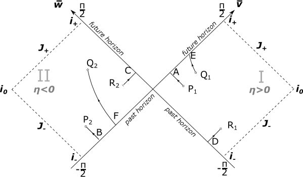
Figure 1: Kruskal-Penrose diagram of the original Einstein-Rosen bridge

• Future horizon in region $I$ is identified with past horizon in region $II$ as:

  $$({\bar{v}},0)\sim({\bar{v}}-\frac{\pi}{2},0)\;.$$ (29)

  Infalling light rays cross from region $I$ into region $II$ via paths $P_{1}\to A\sim B\to P_{2}$ – all the way within finite world-line time intervals (the symbol $\sim$ means identification according to (29)). Similarly, infalling massive particles cross from region $I$ into region $II$ via paths $Q_{1}\to E\sim F\to Q_{2}$ within finite proper-time interval.

• Future horizon in $II$ is identified with past horizon in $I$:

  $$(0,{\bar{w}})\sim(0,{\bar{w}}-\frac{\pi}{2})\;.$$ (30)

  Infalling light rays cross from region $II$ into region $I$ via paths $R_{2}\to C\sim D\to R_{1}$ where $C\sim D$ is identified according to (30).

5 Kruskal-Penrose Formalism for Two-Throat Lightlike Thin-Shell Wormhole

Now we will briefly discuss the extension of the construction of Kruskal-Penrose diagram for the proper Einstein-Rosen bridge wormhole to the case of lightlike “thin-shell” wormholes with two throats. To this end we will consider the physically interesting example of the charge-confining two-throat “tube-like” wormhole studied in hide-confine . It is a solution of gravity interacting with a special non-linear gauge field system and both coupled to a pair of oppositely charged lightlike branes (cf. Eqs.(10)-(11) above).

The full wormhole spacetime consists of three “universes” glued pairwise via the two oppositely charged lightlike branes located on their common horizons:

• Region $I$: right-most non-compact electrically neutral “universe” – exterior region beyond the Schwarzschild horizon of a Schwarzschild-de Sitter black hole;

• Region $II$: middle “tube-like” “universe” of Levi-Civita-Bertotti-Robinson type LC-BR-1 -LC-BR-3 with finite radial-like spacial extend and compactified transverse spacial dimensions;

• Region $III$: left-most non-compact electrically neutral “universe” – exterior region beyond the Schwarzschild horizon of a Schwarzschild-de Sitter black hole, mirror copy of the left-most “universe”.

• Most remarkable property is that the whole electric flux generated by the two oppositely charged lightlike branes sitting on the two “throats” is completely confined within the finite-spacial-size middle “tube-like” universe – analog of QCD quark confinement!

For a visual representation, see Fig.2 hide-confine .

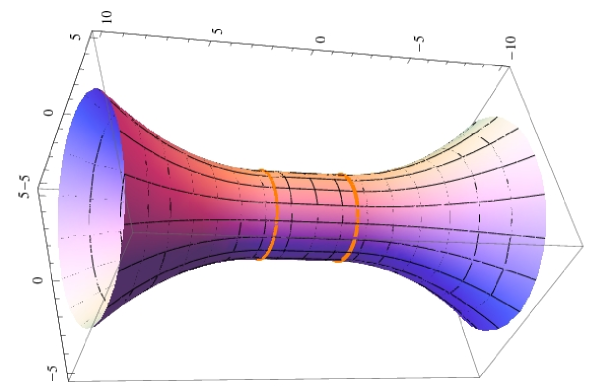
Figure 2: Shape of $t=const$ and $\theta=\frac{\pi}{2}$ slice of charge-confining wormhole geometry. The whole electric flux is confined within the middle cylindric “tube” (region $II$) connecting the two infinite “funnels” (region $I$ and region $III$). The rings on the edges of the “tube” depict the two oppositely charged lightlike branes.

Generically, the metric of a spherically symmetric traversable lightlike thin-shell wormhole with two “throats” reads hide-confine ($-\infty<\eta<\infty$):

$$ds^{2}=-A(\eta)dt^{2}+\frac{d\eta^{2}}{A(\eta)}+r^{2}(\eta)\left(d\theta^{2}+\sin^{2}\theta d\varphi^{2}\right)\;,\phantom{aaaaaaa}$$ (31)

$$A(\eta_{1})=0\;,\;A(\eta_{2})=0\;,\;a^{(1)}_{(\pm)}=\pm\frac{{\partial{}}}{{\partial{\eta}}}A\bigm{|}_{\eta_{1}\pm 0}>0\;,\;a^{(2)}_{(\pm)}=\pm\frac{{\partial{}}}{{\partial{\eta}}}A\bigm{|}_{\eta_{2}\pm 0}>0\;.$$ (32)

Accordingly, for the wormhole “tortoise” coordinate $\eta^{*}$ defined as in first Eq.(18) we have in the vicinity of the two horizons $\eta_{1,2}$:

$$\eta^{*}={\rm sign}(\eta-\eta_{1})a^{(1)}_{(\pm)}\ln|\eta-\eta_{1}|+O\bigl{(}(\eta-\eta_{1})^{2}\bigr{)}\;,$$ (33)

$$\eta^{*}={\rm sign}(\eta-\eta_{2})a^{(2)}_{(\pm)}\ln|\eta-\eta_{2}|+O\bigl{(}(\eta-\eta_{2})^{2}\bigr{)}\;.$$ (34)

Now we can introduce the Kruskal-like and the compactified Kruskal-Penrose coordinates $({\bar{v}},{\bar{w}})$ for the maximal analytic extension of the two-throat lightlike thin-shell wormhole generalizing formulas (23) and (28) as follows:

• In region $I$ (right-most universe) – $(+\infty>\eta>\eta_{1})$:

  $${\bar{v}},{\bar{w}}=\pm\frac{\pi}{2\sqrt{a^{(1)}_{(-)}}}\pm\frac{1}{\sqrt{a^{(1)}_{(+)}}}\arctan\Bigl{(}e^{\frac{1}{2}a^{(1)}_{(+)}(\eta^{*}\pm t)}\Bigr{)}$$ (35)

• In region $II$ (middle universe) – $(\eta_{1}>\eta>\eta_{2})$; here $a^{(1)}_{(-)}=a^{(2)}_{(+)}$ which is satisfied in the case of the charge-confining two-throat “tube” wormhole:

  $${\bar{v}},{\bar{w}}=\pm\frac{1}{\sqrt{a^{(1)}_{(-)}}}\arctan\Bigl{(}e^{\frac{1}{2}a^{(1)}_{(-)}(\eta^{*}\pm t)}\Bigr{)}\;.$$ (36)

• In region $III$ (left-most universe) – $(\eta_{2}>\eta>-\infty)$:

  $${\bar{v}},{\bar{w}}=\mp\frac{\pi}{2\sqrt{a^{(2)}_{(-)}}}\pm\frac{1}{\sqrt{a^{(2)}_{(-)}}}\arctan\Bigl{(}e^{\frac{1}{2}a^{(2)}_{(-)}(\eta^{*}\pm t)}\Bigr{)}\;.$$ (37)

The resulting Kruskal-Penrose diagram is depicted on Fig.3.

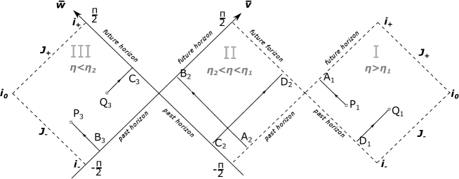
Figure 3: Kruskal-Penrose diagram of “charge-confining” two-throat wormhole

In particular, infalling light ray starting in region $I$ arrives in region $III$ within finite world-line time interval (“proper-time” in the case of massive particle) on the path $P_{1}\to A_{1}\sim A_{2}\to B_{2}\sim B_{3}\to P_{3}$, where the symbol $\sim$ indicates identification of the pertinent future and past horizons of the “glued” together neighboring “universes” analogous to the identification (29), (30) in the simpler case of Einstein-Rosen one-throat wormhole.

And similarly for an infalling light ray starting in region $III$ and arriving in region $I$ within finite world-line time interval on the path $Q_{3}\to C_{3}\sim C_{2}\to D_{2}\sim D_{1}\to Q_{1}$.

6 Conclusions

The mathematically correct reformulation ER-bridge of original Einstein-Rosen “bridge” construction, briefly reviewed in Section 2 above, shows that it is the simplest example in the class of static spherically symmetric traversable lightlike “thin-shell” wormhole solutions in general relativity. The consistency of Einstein-Rosen “bridge” as a traversable wormhole solution is guaranteed by the remarkable special properties of the world-volume dynamics of the lightlike brane, which serves as an “exotic” thin-shell matter (and charge) source of gravity.

In the present note we have explicitly derived the Kruskal-like extension and the associated Kruskal-Penrose diagram representation of the mathematically correctly defined original Einstein-Rosen “bridge” ER-bridge with the following significant differences w.r.t. Kruskal-Penrose extension of the standard Schwarzschild black hole defining the corresponding “textbook” version of Einstein-Rosen “bridge” (the Schwarzschild wormhole) MTW :

• The pertinent Kruskal-Penrose diagram for the proper Einstein-Rosen bridge (Fig.1) has only two regions corresponding to “our” (right) and the second (left) “universes” unlike the four regions in the standard Schwarzschild black hole case (no black/white hole regions).

• The proper original Einstein-Rosen bridge is a traversable static spherically symmetric wormhole unlike the non-traversable non-static “textbook” version. Traversability is equivalent to the pairwise specific identifications of future with past horizons of the neighboring Kruskal regions.

We have also extended the Kruskal-Penrose diagram construction to the case of lightlike “thin-shell” wormholes with two throats.

- (1) C. Barrabés and W. Israel, Phys. Rev. D43 (1991) 1129-1142.
- (2) C. Barrabés and P. Hogan, “Singular Null Hypersurfaces in General Relativity”, (World Scientific 2003).
- (3) C. Barrabés and W. Israel, Phys. Rev. D71 (2005) 064008. (arxiv:gr-qc/0502108)
- (4) E. Guendelman, A. Kaganovich, E. Nissimov, S. Pacheva, Phys. Lett. B673 (2009) 288-292. (arxiv:0811.2882);
- (5) E. Guendelman, A. Kaganovich, E. Nissimov, S. Pacheva, Phys. Lett. B681 (2009) 457-462. (arxiv:0904.3198);
- (6) E. Guendelman, A. Kaganovich, E. Nissimov, S. Pacheva, Int. J. Mod. Phys. A25 (2010) 1405-1428. (arxiv:0904.0401)
- (7) E. Guendelman, A. Kaganovich, E. Nissimov and S. Pacheva, Int. J. Mod. Phys. A25 (2010) 1571-1596. (arxiv:0908.4195)
- (8) E. Guendelman, A. Kaganovich, E. Nissimov and S. Pacheva, Gen. Rel. Grav. 43 (2011) 1487-1513. (arxiv:1007.4893).
- (9) M. Visser, “Lorentzian Wormholes. From Einstein to Hawking” (Springer, Berlin, 1996).
- (10) A. Einstein and N. Rosen, Phys. Rev. 48 (1935) 73.
- (11) Ch. Misner, K. Thorne and J.A. Wheeler, “Gravitation” (W.H. Freeman and Co., San Francisco, 1973).
- (12) E. Guendelman, A. Kaganovich, E. Nissimov and S. Pacheva, Phys. Rev. D72 (2005) 0806011. (hep-th/0507193)
- (13) E. Guendelman, A. Kaganovich, E. Nissimov and S. Pacheva, Fortschritte der Physik 55 (2007) 579. (hep-th/0612091)
- (14) E. Guendelman, A. Kaganovich, E. Nissimov and S. Pacheva, in “Fourth Internat. School on Modern Math. Physics”, ed. by B. Dragovich and B. Sazdovich (Belgrade Inst. Phys. Press, Belgrade 2007), pp.215-228. (hep-th/0703114).
- (15) E. Guendelman, A. Kaganovich, E. Nissimov and S. Pacheva, in “Lie Theory and Its Applications in Physics 07”, ed. by V. Dobrev and H. Doebner (Heron Press, Sofia, 2008). (arxiv:0711.1841)
- (16) E. Guendelman, A. Kaganovich, E. Nissimov and S. Pacheva, Int. J. Mod. Phys. A26 (2011) 5211-5239. (arxiv:1109.0453 [hep-th])
- (17) N. Poplawski, Phys. Lett. 687B (2010) 110-113. (arxiv:0902.1994)
- (18) M.O. Katanaev, Mod. Phys. Lett. A29 (2014) 1450090. (arXiv:1310.7390)
- (19) T. Levi-Civita, Rend. R. Acad. Naz. Lincei, 26, 519 (1917).
- (20) B. Bertotti, Phys. Rev. D116 (1959) 1331.
- (21) I. Robinson, Bull. Akad. Pol., 7, 351 (1959).