We make a first principle calculation of the fragility index $m$ of a simple liquid using the structure of the supercooled liquid as an input. Using the density functional theory (DFT) of classical liquids, the configurational entropy ${\cal S}_{c}$ is obtained for low degree of supercooling. We extrapolate this data to estimate the Kauzmann temperature $T_{\mathrm{K}}$ for the liquid. Using the Adam-Gibbs relation, we link the configurational entropy ${\cal S}_{c}$ to the relaxation time. The relaxation times are obtained from direct solutions of the equations of fluctuating nonlinear hydrodynamics (FNH). These equations also form the basis of the mode coupling theory (MCT) for glassy dynamics. The fragility index for the supercooled liquid is estimated from analysis of the curves on the Angell plot.

Fragility index of a simple liquid from structural inputs

I Introduction

The thermodynamic equilibrium state of a liquid is characterized in terms of a few characteristic variables like temperature $T$, pressure $P$, volume $V$, equilibrium density $\rho_{0}$. The equilibrium liquid state is isotropic in a time averaged sense and the constituent particles have random motion. The isotropic liquid transforms in to a crystalline solid when its temperature $T$ falls below a characteristic value $T_{m}$, termed as the freezing point of the liquid at the corresponding pressure $P$. The isotropic symmetry of the normal liquid state is spontaneously broken at $T_{m}$. The crystalline state has characteristic long range order. The transformation of the liquid in to crystalline solid involves absorption of latent heat. Freezing process is distinct from the condensation of the gaseous state in to the liquid state. The density functional theory (DFT) presents an order parameter theory RY for freezing, using the equilibrium density as the relevant variable. In DFT, the thermodynamic properties of the inhomogeneous crystalline state are obtained in terms of the corresponding properties of the homogeneous liquid state. The thermodynamics of the dense uniform liquid is well understood in a microscopic approach through integral equations theories hansen or simulations. The interaction potential between the liquid particles constitute the microscopic level description of the many particle system. The basic characteristics of the two body potential for which a crystalline state appears (under appropriate conditions of density and temperature) include (a) a strongly repulsive part at short range and an (b) an attractive part effective over long range. The Hamiltonian for the many particle system is written in a harmonic expansion around the equilibrium sites which correspond to the minimum potential energy configuration. The attractive part of the potential seemingly appears to play an important role in stabilizing the solid in a crystalline state in which the individual particles localized around their mean positions.

In the classical DFT, the free energy of an inhomogeneous system is obtained as a functional of the one particle density $\rho({\bf x})$evans_1979 . The density function is expressed in terms of a suitable set of parameters which are treated as the order parameters of the freezing transition. The free energy functional is minimized with respect to these parameters. A very successful prescription of density distribution for the crystalline case is obtained from the superposition of Gaussian density profilesPT centered on a lattice with long range order,

$$\rho(\vec{r})=\sum_{i}\phi_{0}(|\vec{r}-\vec{R}_{i}|)$$ (1)

where the $\{{\vec{R}_{i}}\}$ denotes the underlying lattice and the function $\phi_{0}$ is taken as the isotropic Gaussian $\phi_{0}(r)=(\frac{\alpha}{\pi})^{\frac{3}{2}}e^{-\alpha r^{2}}$. The thermodynamic properties of the system are computed assuming the latter to be in a single phase, i.e., either liquid or crystal. The density functional approach is mean field like since it ignores the effects of fluctuations. At a given density by locating the free energy minimum the corresponding structure is identified as the stable thermodynamic state. For high temperatures, the homogeneous liquid state is more stable while at low temperatures the crystalline state with long range order is more stable. For the simple Lennard-Jones system that we consider here, the face centered cubic (fcc) structure is more stable.

The present paper focuses on the statistical mechanics of liquids below freezing. Almost all liquids can be supercooled with varying degrees of ease, below the freezing point $T_{m}$ without transforming in to an ordered crystalline state. The liquid continues to remain in the amorphous state and its characteristic relaxation time drastically increases with lowering of temperature. The so called glass transition point $T_{\mathrm{g}}$ which denotes the vitrification process, is defined as the temperature at which the relaxation time of the under-cooled liquid reaches the laboratory time scales. The supercooled liquid at this stage behaves like a solid with elastic properties. Unlike freezing process, this transformation is not associated with any latent heat absorption and there is a drop in the specific heat due to absence of the translational degree of freedom. The free energy of the supercooled liquid is expected not to show any discontinuous change through the glass transition. At deep supercooling, liquid can remain trapped in a metastable state having free energy intermediate between the liquid and the crystalline state. Since there are a large number of available metastable structures in which the under-cooled liquid can be trapped, a considerable entropic drive is present for the process. There have been theories for the vitrification process built on possible scenarios of first order transitions with the special situation of a large number of available metastable states mosaic .

An instructive plot of the data of glassy relaxation was made by Angell angell of relaxation time $\tau_{\alpha}$ vs. inverse temperature $T_{\mathrm{g}}/T$ scaled with $T_{\mathrm{g}}$ on a logarithmic scale. The nature of increase of relaxation time with fall of temperature in glassy systems is non-universal. One extreme is a slow growth of $\tau_{\alpha}$ with lowering of temperature $T$ over the temperature range $T>T_{\mathrm{g}}$ followed by very sharp increase within a small temperature range close to $T_{\mathrm{g}}$. A more uniform increase is seen over the whole temperature range for strong liquids like ${\rm B}_{2}{\rm O}_{3}$ or Si${\rm O}_{2}$. This behavior has been quantified by defining a fragility parameter $m$ as the slope of the viscosity-temperature curve as bohmer1 .

$$m=\frac{d\log_{10}{\tau_{\alpha}}}{d(T_{\mathrm{g}}/T)}{\Big{|}}_{T=T_{\mathrm{g}}}~{}~{}.$$ (2)

Thus for example, $o$-terphenyl and Si${\rm O}_{2}$ denote two extreme cases of fragile and strong systems with $m$ values 81 and 20 respectively. At the extreme fragile end the change of relaxation time is extremely dramatic growing by many orders of magnitude within a very narrow temperature range.

The supercooled liquid acts like a frozen solid over time scales of structural relaxation and have only vibrational motion around a frozen structure bpeak-pre ; bpeak-pla . The difference of the entropy of the supercooled liquid from that of the solid having only vibrational motion represents the entropy due to large scale motion of the particles and is identified as the configurational entropy ${\cal S}_{c}$ of the liquid. A rapid disappearance of the configurational entropy of the disordered liquid occurs on approaching the glass transition point. This so called “entropy crisis” poses an important question essential for our understanding the physics of glass transition and the divergence of relaxation time at $T_{\mathrm{g}}$. Apart from having characteristic large viscosity, the supercooled liquid shows a discontinuity in specific heat $c_{p}$ at $T_{\mathrm{g}}$ due to freezing of the translational degrees of freedom in the liquid. The above described features are almost universally observed in all liquids. The Kauzmann temperature $T_{\mathrm{K}}$ is the temperature at which the extrapolated value of ${\cal S}_{c}$ goes to zero and marks a possible limiting temperature for the existence of the supercooled liquid phase. Below $T_{\mathrm{K}}$ we have the paradoxical situation in which the entropy of the disordered state becomes less than that of the crystal. The original hypothesis due to Kauzmann proposes eventual crystallization in the supercooled liquid at very low temperatures as a possible way out. Another possible explanation of the Kauzmann paradox could be that the simple extrapolation of high temperature result to very low temperature is not correct and the entropy difference between supercooled liquid and crystal remains finite till very low temperature Langer_2007 ; Donev_2006 , finally going to zero only near $T=0$.

The theory of the supercooled liquid primary deals with two broad aspects of the metastable state. These respectively refer to the thermodynamics property like the configurational entropy and the slow dynamics characteristic of the glassy state. With increased supercooling the relaxation time for the liquid sharply increases. Relaxation in the present context is meant for a typical fluctuation around the disordered liquid state at a temperature $T<T_{m}$. Dynamics of the deeply supercooled liquid changes over from a continuous motion of its particles to transport by activated hopping over barriers that develops at low temperature. In structural glass this occurs even without any quenched impurities, i.e., the slow dynamics is self generated. In the Adam-Gibbs theory agibbs the growth of the relaxation is linked to the configurational entropy ${\cal S}_{c}$ of the supercooled liquid. The idea that energy barriers build up to resist molecular rearrangement in the jammed state has been used in the Adam-Gibbs theory to understand the development of very long relaxation times in the deeply supercooled state dim-cdg . Since relaxation in the system occurs through thermally assisted hopping over the barrier (=$E_{B}$ say), the probability of such a jump will be controlled by the Boltzmann factor $\exp(-E_{B}/k_{B}T)$. Thus estimation of the relaxation time is closely linked to that of the energy barrier $E_{B}$ which must be overcome so that a local fluctuation can relax. Using these ideas it is argued agibbs that the relaxation time $\tau$ is linked to the configurational entropy ${\cal S}_{c}$ at temperature $T$ of the liquid through the relation

$$\tau=\tau_{0}\exp\left[\frac{A_{0}}{T{\cal S}_{c}}\right]~{}~{},$$ (3)

where $A_{0}$ is a constant. As $T{\rightarrow}T_{\mathrm{K}}$, the configurational entropy ${\cal S}_{c}\rightarrow{0}$ and hence $\tau{\rightarrow}\infty$. Thus assuming a linear temperature dependence of $T{\cal S}_{c}$ near $T_{\mathrm{K}}$ we can identify $T_{\mathrm{K}}$ with the temperature $T_{0}$ of the standard Vogel-Fulcher dependence of relaxation $\tau=\tau_{0}\exp(A/(T-T_{0})$ vogel . This equality between $T_{0}$ and $T_{\mathrm{K}}$ suggests a link of deeper significance on considering the fact that the physics of the two temperatures are very different. $T_{0}$ represents the temperature at which the relaxation time for the supercooled liquid diverges and basically relates to the dynamics. On the other hand the Kauzamann temperature $T_{\mathrm{K}}$ is related to the vanishing of the thermodynamic property of configurational entropy of the metastable liquid. Linking of the sharp in crease of relaxation time to the entropy crisis signifies effects of structure on the dynamics entr-jcp .

For studying the classical liquid at densities beyond freezing point, the DFT ys-pr ; lowen-pr ; mybook-cam and the MCT my_rmp ; reichman-chr has been two primary tools. In the present paper we use of both approaches to study the properties of the supercooled liquid. The density functional methods has been adopted for studying the thermodynamic properties of the liquid while mode coupling theories offers a microscopic model for slow dynamics of the metastable liquid approaching glass transition. In its simplest form the theory predicts a sharp dynamic transition around a temperature $T_{c}$ higher than $T_{\mathrm{g}}$. This is a transition from the ergodic liquid state to a nonergodic state in which long time limits of the density correlation function does not decay to zero. Around $T_{c}$, scaling behavior the dynamics of the liquid undergoes a qualitative change. Using only structural inputs, scaling of the non ergodicity parameter cusp_jcp and growing dynamic length scale dlength ; biroli-epl have been studied around the MCT transition point.

Similar to the studies of the freezing transition, the DFT methods have been applied to model the supercooled liquid below the freezing point $T_{m}$, having aperiodic structures ysingh ; dasgupta_1992 ; PRL_DFT . The inhomogeneous states are characterized by localized density profiles (over suitable time scales) around a disordered set of lattice points. For the aperiodic structure, the corresponding $\{{\bf R}_{i}\}$ in the definition (1) for the density constitute a random structure. The quantity $\alpha$ in Eq. (1) is the variational parameter chandan-sood . Inverse of $\alpha$ characterizes the width of the peak and therefore signifies the degree of mass localization in the system. The homogeneous liquid state is characterized by the limit $\alpha{\rightarrow}0$ and each Gaussian profile provides the same contribution in the sum at all spatial positions. The metastable states are identified as minima of the free energy, intermediate between a crystal and a homogeneous liquid state.

Next we consider the model for understanding the dynamics, i.e., the mode coupling models. Recently the relaxation time of a simple liquid has been calculated pre_barrat from a direct solution of the equations of fluctuating nonlinear hydrodynamics (FNH). These equations are also the starting point of mode coupling theory. On the other hand using the density functional methods we compute here the configurational entropy ${\cal S}_{c}$ in the region close to $T_{m}$. In the present paper we use the temperature dependence of the relaxation time and the Adam-Gibbs relation involving the configurational entropy ${\cal S}_{c}$ (in the higher temperature range) to estimate the fragility index of a simple Lennard-Jones liquid. ${\cal S}_{c}$ is estimated using the structure of the liquid. Hence the present calculation only requires as an input the basic interaction potential in terms of which the structure factors are obtained. The paper is organized as follows. In Sec. II, we present the respective models studied for the thermodynamics and the dynamics separately. In Sec. III the numerical results obtained for the configurational entropy is checked for the validity of the Adam-Gibbs relation with the use of the relaxation time. We then explore the Angell plots of the model studied. The paper ends with a discussion section.

II Model studied

We are dealing in this paper with two types of microscopic models for the description of the metastable liquid. First, the density functional model which provides a description of the properties related to thermodynamics. Second, the equations of fluctuating nonlinear hydrodynamics for the supercooled liquid signifying the underlying conservation laws for the many particle system. We briefly describe these two approaches in this section.

II.1 Model for thermodynamics

First we briefly outline the construction of the proper free energy functional $F[\rho]$ corresponding to the ensemble in which the average density is computed. This functional is then used to determine the appropriate parameters for the inhomogeneous density function $\rho({\bf x})$ at equilibrium. This is done by satisfying the extremum principle for $F[\rho]$. For the canonical ensemble it is the Helmoholtz free energy functional $F[\rho]$ which is to be minimized to identify the equilibrium state. The free energy of the liquid is obtained as a sum of two parts - the ideal gas term and the interaction term,

$$F[\rho]=F_{\mathrm{id}}[\rho]+F_{\mathrm{ex}}[\rho].$$ (4)

The ideal gas part of the free energy $F_{id}$ for the non-uniform density is obtained as

$$F_{id}[\rho({\bf r})]=k_{B}T\int d{\bf r}\rho({\bf r})\left(\ln[\wedge^{3}\rho({\bf r})]-1\right).$$ (5)

$\wedge$ represents the thermal wavelength appearing due to the momentum variable integration in the partition function. The RHS of Eq. (5) is a simple generalization of the ideal gas part of the free energy for the nonuniform density, i.e., $\rho\rightarrow\rho(x)$. The interaction part is evaluated using the standard expression for the Ramakrishnan-Yussouff (RY) functional RY involving a functional Taylor series expansion in terms of the density fluctuation $\delta\rho(\vec{r})=\rho(\vec{r})-\rho_{o}$ around liquid phase of average density $\rho_{o}$,

$$F_{\mathrm{ex}} = F_{\mathrm{ex}}(\rho_{0})-\int d{\bf x}_{1}c^{(1)}({\bf x}_{1};\rho_{0})\delta\rho({\bf x})$$

$$- \frac{1}{2}\int d{\bf x}_{1}\int d{\bf x}_{2}c^{(2)}({\bf x}_{1},{\bf x}_{2};\rho_{0})\delta\rho({\bf x}_{1})\delta\rho({\bf x}_{2})+..$$

The series involve the functions $c^{(i)}$’s defined in (7) at the liquid state density $\rho({\bf x})=\rho_{0}$. For a uniform homogeneous liquid, $\rho_{0}$ will be independent of position. We use the following definitions for the direct correlation functions $c^{(i)}$s as the successive functional derivatives of $F_{\mathrm{ex}}$ evaluated at the liquid state density $\rho_{0}$,

$$c^{(i)}({\bf x}_{1},...,{\bf x}_{i};\rho_{0})=-\left[\frac{\delta^{i}F_{\mathrm{ex}}}{\delta\rho({\bf x}_{1})...\delta\rho({\bf x}_{i})}\right]_{\rho=\rho_{0}}$$ (7)

For practical calculations one usually adopts the simplest approximation keeping only up to the second order term ($i=2$) in the expansion for the direct correlation function. The functional extremum principle now reduce to the form for the canonical ensemble as

$$\ln[\wedge^{3}\rho({\bf x})]-c^{(1)}({\bf x};\rho({\bf x}))+\beta\phi=0~{}~{},$$ (8)

where $\phi({\bf x})$ is the external potential. Using the result (8) we obtain for the equilibrium density $\rho({\bf x})$

$$\rho({\bf x})=z\exp[-\beta\phi({\bf x})+c^{(1)}({\bf x};\rho_{0}({\bf x}))]~{}~{},$$ (9)

where $z=\wedge^{-3}$ in this case. The quantity $c^{(1)}({\bf x};\rho({\bf x}))$ acts as a one body potential due to the interaction between the fluid particles. The higher order direct correlation functions are defined in terms of functional derivatives of $c^{(1)}$ with respect to $\rho({\bf x})$. Making a simple Taylor expansion for $c^{(1)}({\bf x};\rho({\bf x}))$ around its value $c_{l}$ in the uniform liquid state of density $\rho_{0}$, we obtain,

$$c^{(1)}[{\bf x}_{1};\rho({\bf x}_{1}] = c_{l}(\rho_{0})+\int d{\bf x}_{2}c^{(2)}[{\bf x}_{1},{\bf x}_{2};\rho_{0}]\delta\rho({\bf x}_{2})$$

$$+ \frac{1}{2}\int d{\bf x}_{2}d{\bf x}_{3}c^{(3)}[{\bf x}_{1},{\bf x}_{2},{\bf x}_{3};\rho_{0}]\delta\rho({\bf x}_{2})\delta\rho({\bf x}_{3})+....$$

where $\delta\rho({\bf x})=\rho({\bf x})-\rho_{0}$ is the fluctuation of the equilibrium density in the inhomogeneous solid state from that of the liquid state. The two point function function $c^{(2)}({\bf x}_{1},{\bf x}_{2})$ is related to the pair correlation function $g^{(2)}({\bf x}_{1},{\bf x}_{2})$ in the fluid by a relation which reduces to the Ornstein-Zernike relation for the uniform liquid. For the uniform liquid in absence of any external field we have from Eq. (9) for the uniform density $\rho_{0}=z\exp(c_{l})$. The inhomogeneous density function $\rho({\bf x})$ is then obtained in terms of the corresponding one particle direct correlation function $c^{(1)}(r)$,

$$\rho({\bf x})=\rho_{0}\exp\left\{c^{(1)}({\bf x};\rho({\bf x}))-c_{l}-\beta\phi({\bf x})\right\}~{}~{}.$$ (11)

The equilibrium density is therefore obtained as

$$\rho({\bf x}_{1})=\bar{\rho}_{0}({\bf x}_{1})\exp\left[\int d{\bf x}_{2}c^{(2)}({\bf x}_{1},{\bf x}_{2};\rho_{0})\delta\rho_{0}({\bf x}_{2})\right]$$ (12)

where we identify $\bar{\rho}_{0}({\bf x})=z\exp[-\beta\phi({\bf x})+c_{l}({\bf x})]\equiv\rho_{0}\exp[-\beta\phi({\bf x})]$. For Eq. (12) the trivial solution is then the uniform density $\rho({\bf x}_{1})=\rho_{0}$ in absence of any external field $\phi$. The solution of Eq. (12) is the starting point for the subsequent analysis for testing the possibility of an inhomogeneous density state. The two point kernel function $c^{(2)}({\bf x}_{1},{\bf x}_{2};\rho_{0})$ which is defined in terms of the functional derivative of the one body potential $c^{(1)}$ is required to completely specify the equation (12) for the inhomogeneous density.

II.2 Appropriate free energy functional

The density functional which is minimized with respect to the density functions $\rho({\bf x})$ is obtained here for the constant $NVT$ ensemble. Both the homogeneous and the inhomogeneous states are at the same temperature and volume and number of particles. The corresponding thermodynamic potential which is minimized is the Helmholtz free energy. The difference between the free energy functionals in the inhomogeneous state with density $\rho({\bf x})$ and the homogeneous liquid state with density $\rho_{0}$ ( in absence of the external potential $\phi({\bf x})$) is obtained as,

$$\Delta{\cal F} \equiv {\cal F}[\rho({\bf x})]-{\cal F}[\rho_{0}]=\Delta F_{\mathrm{id}}[\rho({\bf x})]+\Delta F_{\mathrm{ex}}[\rho({\bf x})]$$ (13)

$$+ \int d{\bf x}_{1}(\rho(x_{1})-\rho_{0})\phi(x_{1}).$$

The difference $\Delta F_{\mathrm{id}}=F_{\mathrm{id}}[\rho({\bf x})]-F_{\mathrm{id}}(\rho_{0})$ in the ideal gas part of the free energy is directly calculated from (33). The difference $\Delta F_{\mathrm{ex}}=F_{\mathrm{ex}}[\rho({\bf x})]-F_{\mathrm{ex}}(\rho_{0})$ between the excess free energies of the liquid and solid states is expressed as a functional Taylor expansion in the density fluctuations $\delta\rho({\bf x})=\rho({\bf x})-\rho_{0}$ from (II.1). Using these results, we obtain the free energy difference between the crystalline and liquid state as,

$$\Delta{\cal F} = \int d{\bf x}_{1}\Bigg{[}\rho({\bf x}_{1})\ln\left[\frac{\rho({\bf x}_{1})}{\rho_{0}}\right]-{\delta}\rho({\bf x}_{1})\left\{1+\ln(\rho_{0}\wedge^{3})-c^{(1)}({\bf x}_{1};\rho_{0})+\phi(x_{1})\right\}\Bigg{]}$$ (14)

$$- \frac{1}{2}\int d{\bf x}_{1}\int d{\bf x}_{2}c^{(2)}({\bf x}_{1},{\bf x}_{2};\rho_{0})\delta\rho({\bf x}_{1})\delta\rho({\bf x}_{2})-...$$

$$= \int d{\bf x}_{1}\Bigg{[}\rho({\bf x}_{1})\ln\left[\frac{\rho({\bf x}_{1})}{\rho_{0}}\right]-\frac{1}{2}\int d{\bf x}_{1}\int d{\bf x}_{2}c^{(2)}({\bf x}_{1},{\bf x}_{2};\rho_{0}){\delta}\rho({\bf x}_{1}){\delta}\rho({\bf x}_{2})\Bigg{]}~{}~{}~{}.$$

In reaching the above equation we have applied the extremum condition (8) for the liquid state i.e.,

$$\ln\rho({\bf x}_{1})-c^{(1)}({\bf x};\rho_{0})+\phi(x)=0$$ (15)

as well as the fact that for the canonical ensemble the total number of particles are constant.

The procedure followed to compute the free energy for the supercooled liquid would be to first identify the minimum of the $\Delta{\cal F}$ with respect to $\alpha$ since the $\alpha{\rightarrow}0$, the value of ${\cal F}$ is the liquid state free energy. Once the optimum $\alpha$ is identified the corresponding value of ${\cal F}$ for the optimum density gives the free energy for the inhomogeneous state to leading order in density fluctuations.

II.3 Model for the Dynamics

The slow dynamics of a dense liquid is generally studied in terms of the correlation of density fluctuations which occur in the strongly interacting many particle system. The structural relaxation is best understood in terms of the two point dynamic correlation function ${C}(q,t_{1},t_{2})$ of density fluctuations at times $t_{1}$ and $t_{2}$, corresponding to wave vector $q$. The correlation function is defined in the normalized form

$${C}(q,t_{1},t_{2})=\frac{<\delta\rho(q,t_{1})\delta\rho(-q,t_{2})>}{<\delta\rho(q,t_{2})\delta\rho(-q,t_{2})>}~{}~{}.$$ (16)

For the equilibrium state, time translational invariance holds and $C(t_{1},t_{2})$ is a function of $(t_{1}-t_{2})$ only. The long time limit of the time correlation of density fluctuations is treated as an order parameter in the mode coupling theory (MCT) of glassy dynamics. This quantity, termed as the nonergodicity parameter (NEP), makes a discontinuous jump from being zero in the liquid state to a nonzero positive value at the ergodic-nonergodic (ENE) transition of MCT. The corresponding temperature $T_{c}$ identified with the sharp transition signifies a point at which a qualitative change occurs in the moderately supercooled regime. $T_{c}$ lies in a temperature range between the freezing temperature $T_{m}$ and the glass transition temperature $T_{\mathrm{g}}$. The sharp ENE transition is smoothed off in a complete analysis of the nonlinearities in the equations which control the dynamics of density fluctuations. However the qualitative change in the dynamics in the initial stages of supercooling, around $T_{c}$ are described in terms of the basic equations of FNH. The model equations of MCT also follows from these equation which are plausible generalizations of equations of hydrodynamics extended to small wave lengths. These equations have been solved numericallypre_barrat ; cdg_valls and the relaxation times obtained are in good agreement with simulations results on similar systems.

For an isotropic liquid, the model equations of FNH for the mass density $\rho$ and momentum density gDM in the simplest form are as follows :

$$\frac{\partial\rho}{\partial{t}}+{\bf\nabla}.{\bf g}=0,$$ (17)

$$\frac{\partial g_{i}}{\partial t}+\rho\nabla_{i}f(r,t)-L_{ij}\frac{g_{j}}{\rho}=\theta_{i}~{}~{}.$$ (18)

The correlations of the Gaussian noise $\theta_{i}$ are related to the bare damping matrix $L^{0}_{ij}$ boon-yip ,

$$\left\langle\theta_{i}(x,t)\theta_{j}({x^{\prime}}t^{\prime})\right\rangle=2k_{B}TL^{0}_{ij}\delta(t-t^{\prime})\delta(x-x^{\prime}).$$ (19)

For an isotropic liquid, the bare transport coefficients are obtained as,

$$L^{0}_{ij}=(\zeta_{0}+\eta_{0}/3)\delta_{ij}\nabla^{2}+\eta_{0}\nabla_{i}\nabla_{j}$$ (20)

where $\zeta_{0}$ and $\eta_{0}$ respectively denote the bare bulk and shear viscosities. For the glassy dynamics we focus on the coupling of slowly decaying density fluctuations present in the pressure functional, represented by the second term on the LHS of Eq. (18). The nonlinear contribution in this term is obtained with the function $f(r,t)$. The latter is presented as a convolution

$$f(\textbf{r},t)=m^{-1}\int d\textbf{r}c(\textbf{r}-\textbf{r}^{{}^{\prime}})\delta\rho(\textbf{r}^{{}^{\prime}},t).$$ (21)

If we replace $\rho$ by $\rho_{0}$ in the RHS of Eq. (18) then we have a dynamics linearized in density fluctuations. The above described FNH equations are solved numerically on a grid. The direct correlation function $c(r)$ is used as an input for solving the FNH equations and the noise averaged correlation function $C(q,t)$ of density fluctuations are obtained pre_barrat . With the thermodynamic property, i.e., the free energy ${\cal F}$ being known using the classical DFT methods outlined above and the dynamics properties i.e., relaxation time obtained from the solutions of the equations of FNH, the Adam-Gibbs relation can be tested near the temperature $T_{c}$.

III Numerical results

In DFT, the free energy is expressed as a functional of the density $\rho({\bf x})$ which incorporates two key properties of the solid state. First, the extent of mass localization in the system is denoted by the width parameter $\alpha$ defined in the Eq. (1). Second, the underlying lattice $\{{\bf R}_{i}\}$ on which the Gaussian density profiles are to be centered. Both of these properties are treated as control parameters of DFT.

For our analysis, we consider here a classical system of $N$ particles, each of mass $m$ interacting with a Lennard-Jones potential

$$u(r)=4\epsilon\left[{\left(\frac{\sigma}{r}\right)}^{12}-{\left(\frac{\sigma}{r}\right)}^{6}\right].$$ (22)

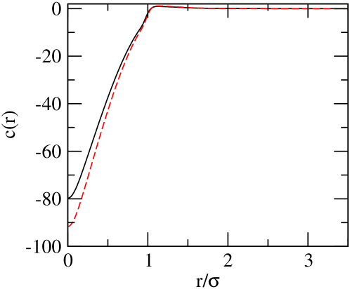
Figure 1: The direct correlation function at temperature $T=1$ (solid line) and $.8$ (dashed line) for density $\rho_{0}{\sigma^{3}}=1.1$.

The basic interaction potential in Eq. (22) defines the length scale $\sigma$ and energy scale $\epsilon$ used in defining the units of density and temperature. The equilibrium density and the temperature of the LJ system in the present paper will be respectively expressed in units of $\sigma^{-3}$ and $\epsilon/k_{B}$. The structure of the corresponding homogeneous liquid, denoted by $c(r)$ is a required input in the calculation. For the LJ potential, the direct correlation function of the uniform liquid is obtained using the bridge function method bridge-fn-lj ; bridge-fn-lj-96 .The thermodynamic properties of the supercooled liquid are obtained using the constant NVT ensemble of $N$ particles interacting with the LJ potential in volume $V$ and has a constant temperature $T$. In Fig. 1 we show the direct correlation function $c(r)$ obtained for density $\rho_{0}\sigma^{3}=1.1$. The corresponding temperatures are $k_{B}T/\epsilon=0.8$ and $1.0$. Next, we consider the distribution of particle sites $\{{\bf R}_{i}\}$. In case of crystal, FCC lattice serves as the particle sites. For the amorphous glassy states, the centers for the Gaussian density profiles $\{{\bf R}_{i}\}$ in the expression (1) for the density function are assumed to be distributed on a random lattice. A standard procedure generally followed ysingh ; baus-colot ; lowen-90 here to obtain the random structure is to use the $g_{B}(R)$ corresponding to the Bernal’s packing Bernal_1964 which is generated through the Bennett’s algorithm Bennett_algorithm . We use the random structure $g_{s}(R)$ through the following relation baus-colot

$$g_{s}(R)=g_{B}~{}[{\gamma_{0}}R]~{}~{},$$ (23)

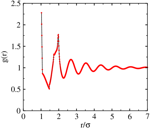
Figure 2: The Bernal pair correlation function $g_{B}(r)$ vs. $r/\sigma$ where $\sigma$ is the microscopic scale of the interaction potential.

with $\gamma_{0}={({\eta}/{\eta_{0}})}^{1/3}$ where $\eta$ denotes the average packing fraction. $\eta_{0}$ is used as a scaling parameter for the structure such that at $\eta=\eta_{0}$ Bernal’s structure $g_{B}(R)$ is reproduced. The mapping of the function from $g_{s}(R)$ to $g_{B}(\gamma_{0}{R})$ makes the structure represented by $g_{s}$ to become more spread apart with increasing $\eta_{0}$, at a fixed packing fraction $\eta(<\eta_{0})$. The role of the $\eta_{0}$ on the free energy landscape plays a crucial role in this work. We display in Fig. 2 the Bernal’s random structure. In this regard it should be noted that for a hard sphere system identification of the most closely packed random structure is somewhat anomalous Torquato_2000 . In the present context, however, the Bernal structure is simply applied as a tool to evaluate the free energy for an inhomogeneous density profile centered at the random set of lattice points.

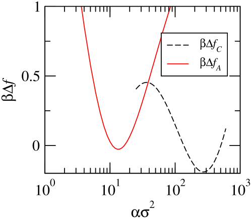
Figure 3: Total free energies Vs. width parameter are shown for density $\rho_{0}^{*}=1.1$. We locate the thermodynamically preferred metastable glassy states w.r.t. the localization parameter $\alpha$ for two different structures: Bernal’s random structure (solid line) and fcc lattice sites (dashed line).

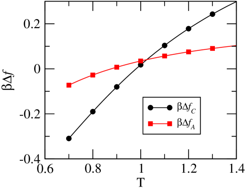
Figure 4: Difference of the free energy $\Delta{f}$ of the amorphous glassy state (solid) and fcc crystalline state (dashed) respectively from that of the uniform liquid vs. temperature $k_{B}T/\epsilon$, at constant density $\rho_{0}{\sigma^{3}}=1.1$.

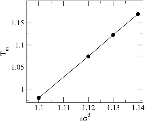
Figure 5: The freezing temperature $T_{m}$ ( in units of $\epsilon/k_{B}$) vs. density $\rho_{0}\sigma^{3}$.

Using the above formulas and the input structure for the uniform liquid in terms of $c(r)$ and the random structure $\{{\bf R}_{i}\}$ from the Bernal pair correlation function, the free energy is calculated as a function of the width parameter $\alpha$. The free energy minimum at a given temperature $T<T_{m}$ corresponds to a metastable state with amorphous structure lying in the supercooled regime. The free energy minimization with respect to $\alpha$ is displayed in Fig. 3 for two specific cases displaying the crystalline and the amorphous metastable state. Note that the metastable amorphous structure corresponds to a much lower degree of mass localization compared to the crystalline state. The difference of the free energy of the amorphous or the crystalline state from that of the uniform liquid state are respectively denoted by $\Delta{\cal F}_{\mathrm{a}}$ and $\Delta{\cal F}_{\mathrm{c}}$. The signs of these quantities mark the relative stability of the respective inhomogeneous state with respect to the homogeneous liquid state. In Fig. 4 we show that $\Delta{\cal F}_{\mathrm{c}}$ become negative at temperature $T_{m}=0.98$ (shown with an arrow) marking the freezing point. The amorphous state becomes metastable compared to the liquid state at a little lower temperature. For different choices of density $\rho_{0}\sigma^{3}$ of the liquid, we obtain the corresponding $T_{m}$ as shown in Fig. 5.

III.1 Configurational Entropy

The metastable amorphous state distinct from the uniform liquid state, is identified by locating the intermediate minimum of the corresponding free energy with respect to the mass localization parameter $\alpha$. The latter determines the width of the Gaussian density profiles in Eq. (1). For different temperatures, using Eq. (14) we now find the optimum free energy differences $\Delta{\cal F}_{\mathrm{a}}$ and $\Delta{\cal F}_{\mathrm{v}}$, respectively corresponding to the amorphous (metastable) and the crystalline (thermodynamically stable) structure. For the metastable states we use the Bernal’s structure to construct the random lattice $\{{\bf R}_{i}\}$. Different set of lattice points are produced by varying the scaling parameter $\eta_{0}$ introduced in defining the pair correlation function for the random structure. The set of $\eta_{0}$ values are taken as synonymous to different species of glass forming materials. For the crystalline structure $\Delta{\cal F}_{\mathrm{v}}$ is the difference of the free energies of the crystal and uniform liquid state. For the crystalline state we use the fcc lattice to define the underlying points $\{{\bf R}_{i}\}$. The configurational entropy ${\cal S}_{c}$ in the temperature range close to $T_{c}$ is obtained as

$${\cal S}_{c}={\cal S}_{\mathrm{a}}-{\cal S}_{\mathrm{v}}=-\frac{\partial}{\partial T}{\Bigg{|}}_{V}\left[\Delta{\cal F}_{\mathrm{a}}-\Delta{\cal F}_{\mathrm{v}}\right]~{}~{}.$$ (24)

The difference between the entropies of the amorphous state with a weak degree of mass localization ( $\alpha\sigma^{2}{\sim}10^{1}$) and the crystalline state with sharply localized mass distribution ( $\alpha\sigma^{2}{\sim}10^{3}$) is taken here as the configurational entropy.

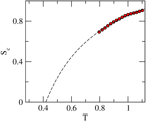
Figure 6: Configurational entropy ${\cal S}_{c}$ Vs. $\bar{T}$ ($=T/T_{m}$) at $\rho_{0}^{*}=1.1$ for amorphous structure as given by $\eta_{0}=.69$. The data is extrapolated by a fit (25) to obtain the corresponding $T_{\mathrm{K}}$.

In the numerical calculation, by using the free energies for the amorphous and crystalline structures for this constant NVT ensemble, we obtain the entropy ${\cal S}_{\mathrm{a}}$, of the supercooled liquid state. At constant density $\rho_{0}\sigma^{3}=1.1$, we obtain the ${\cal S}_{c}$ for a set of values for the parameter $\eta_{0}=.67,.68,.69$, and $.70$. The configurational entropy studied in this density functional model is extrapolated beyond the studied temperature range as shown in Fig. 6 with the form

$${\cal S}_{c}={\cal S}_{0}\left(1-\frac{T_{\mathrm{K}}}{T}\right)~{}~{}.$$ (25)

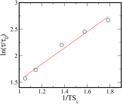
Figure 7: Relaxation time $\ln[\tau/\tau_{0}]$ obtained from the equations of NFH in Ref. pre_barrat vs $T{\cal S}_{c}$. Applicability of Adam-Gibbs relation given by the solid line.

For various $\eta_{0}$, we obtain by fitting the ${\cal S}_{c}$ to the above form the corresponding $T_{\mathrm{K}}$ as well as ${\cal S}_{0}$. To test the Adam-Gibbs relation we use the result for the relaxation time $\tau$ obtained from the solution of the FNH equations pre_barrat . The input structure factor for the liquid used in solving the FNH equations are same as those used in computing the ${\cal S}_{c}$ in the density functional models. The relaxation time $\tau$ is then linked to the configurational entropy ${\cal S}_{c}$ via AG relation so that the $\ln[\tau/\tau_{0}]$ vs. $1/T{\cal S}_{c}$ plot is taken as the best fit to a straight line. This is displayed in Fig. 7. Fitting each set of the configurational entropy data (corresponding to a specific choice of the parameter $\eta_{0}$) the Adam-Gibbs line and hence the slope $A_{0}$ for each $\eta_{0}$ value is obtained. Thus $A_{0}$, ${\cal S}_{0}$ and $T_{\mathrm{K}}$ are obtained for each $\eta_{0}$. Using these we determine for the system characterized by the structure parameter $\eta_{0}$, the corresponding fragility index $m$ on the Angell plot.

III.2 Angell plot

The plot of the glassy relaxation time $\tau$ (on a logarithmic scale) vs. the corresponding inverse temperature $T_{\mathrm{g}}/T$, (scaled with the glass transition temperature $T_{\mathrm{g}}$) is referred to as the Angell plot angell ; turnbull . Here the temperature $T_{\mathrm{g}}$ is defined to be the one at which the relaxation time grows by a chosen order of magnitudes ${\cal B}$ (say) compared to its short time value for any specific system. The quantity ${\cal B}$ is same for all materials and generally it is chosen to be $16$ bohmer1 ; bohmer2 . A given curve on the Angell plot is linked with the configurational entropy ${\cal S}_{c}$ of the system using the Adam-Gibbs relation.

As indicated above, we have already estimated $T_{\mathrm{K}}$ independently from the structural data, i.e., by an extrapolation of the fit of the configurational entropy data obtained at higher $T$ (near $T_{m}$) with the function given by (25). Using this form of ${\cal S}_{c}$ the Adam-Gibb’s relation obtains

$$\tau=\tau_{0}\exp\left[\frac{A_{0}}{{\cal S}_{0}\left(T-{T_{\mathrm{K}}}\right)}\right].$$ (26)

The relaxation time data is expressed as a function of the scaled temperature $x=T_{\mathrm{g}}/T$ with the relation,

$$\ln\left[\frac{\tau}{\tau_{0}}\right]={\cal C}_{0}\frac{x}{\kappa-x}~{}~{}~{}.$$ (27)

We have defined the quantities ${\cal C}_{0}$ and $\kappa$ respectively as

$${\cal C}_{0} = \frac{A_{0}}{{{\cal S}_{0}}T_{\mathrm{K}}}$$ (28)

$$\kappa = {T_{\mathrm{g}}}/{T_{\mathrm{K}}}~{}~{}.$$ (29)

Using the relaxation data obtained from the solution of FNH equations pre_barrat , the constant ${\cal C}_{0}$ is calculated. For every choice of the parameter $\eta_{0}$ which characterize the structure of a particular glass forming system in the DFT model, a corresponding $C_{0}$ is obtained. At $T=T_{\mathrm{g}}$, i.e., $x=1$ we obtain,

$${\cal B}=\ln\frac{\tau}{\tau_{0}}{\Big{|}}_{T=T_{\mathrm{g}}}=\frac{{\cal C}_{0}}{\kappa-1}~{}~{}.$$ (30)

The fragility index $m$ defined in Eq. (2) is obtained by calculating the derivative of the Angell curve given in Eq. (27) at $T=T_{\mathrm{g}}$, i.e., $x=1$.

$$m=\frac{\kappa{\cal C}_{0}}{{(\kappa-1)}^{2}}.$$ (31)

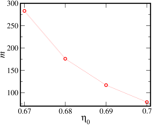
Figure 8: The fragility index $m$ vs. $\eta_{0}$ introduced in Eq. (23).

In Fig. 8 we display the fragility index $m$ vs. the corresponding $\eta_{0}$ characterizing the different structures. The figure shows that less fragile systems have higher characteristic $\eta_{0}$ values, making the gaussian centers more spread out. This represents a structure with sharply localized particles and is more robust for the stronger liquid in which structural degradation is hindered. To summarize the procedure, we read ${\cal S}_{0}$ and $T_{\mathrm{K}}$ from the extrapolation of ${\cal S}_{c}$ as shown in Fig. 6. $A_{0}$ is obtained as a fitting parameter in Fig. 7. The latter involves fitting respective data of relaxation time (from solution of FNH equations) and configurational entropy (from DFT) with the Adam-Gibbs relation. Using these, the constant ${\cal C}_{0}$ defined in Eq. (28) is obtained for the corresponding $\eta_{0}$. For a chosen value of ${\cal B}$, the relation (30) determine the $\kappa$ for a corresponding ${\cal C}_{0}$. Each pair of $\{{\cal C}_{0},\kappa\}$ is obtained for a chosen $\eta_{0}$. The underlying structures $\{{\bf R}_{i}\}$ used in computing the configurational entropy ${\cal S}_{c}$ of the supercooled liquid correspond to chosen $\eta_{0}$ defined in Eq. (23).

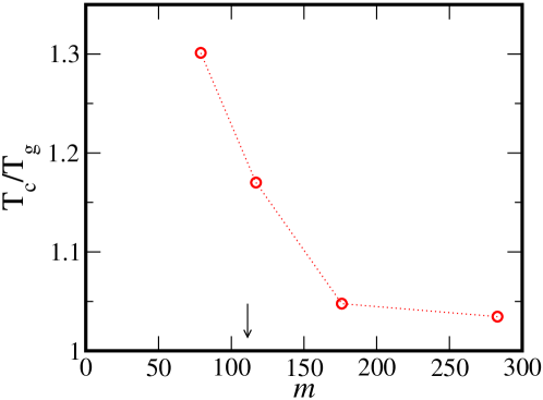
Figure 10: $T_{\mathrm{c}}/T_{\mathrm{g}}$ vs. fragility index $\bar{m}$. The arrow indicates the point at which the ratio is $1.3$.

Using the above result an Angell-plot of $\ln[\tau/\tau_{0}]$ vs. $x$ corresponding to a chosen ${\cal B}=16$ is shown in Fig. 9. The different curves are characterized by respective values of fragility $m$. The fragility is obtained using Eq. (31). The different curves correspond to a set of $\eta_{0}$ values. On the same plot we display the $\tau/\tau_{0}$ data for the Lennard-Jones system obtained from the solutions of the equations of FNH. The fragility $m$ for any particular curve on the Angell plot in Fig. 9 is determined by the $\{\kappa,{\cal C}_{0}\}$. Thus we obtain $m$ for a chosen value of $\eta_{0}$. The high temperature part (low values of $x$) of each of the curves on the Angell plot in Fig. 9 fits well to a power law divergence $(T-T_{c})^{-a}$, with a corresponding set of $\{{T_{c}},a\}$. For each curve on the Angell plot the corresponding glass transition temperature $T_{g}$ is different. Since $T_{\mathrm{K}}$ is known, $T_{\mathrm{g}}$ is obtained using Eq. (30). The ratio $T_{c}/T_{g}$ vs. fragility index $m$ is shown Fig. 10 and its inset. The agreement with experimental results of $T_{c}/T_{g}=1.2$ my_rmp is reached for $m=117$ corresponding to choosing an underlying structure with $\eta_{0}=.69$. This is indicated with an arrow in Fig. 10.

IV Discussion

In all its simplicity, the AG relation glues together two important basic properties of glassy systems, respectively related to the dynamics and the thermodynamics, making the liquid’s relaxation time to be driven by the configurational entropy. In this work, features of the configurational entropy of the glass physics is studied within the framework of density functional theory for the classical liquids. Generally classical DFT has been widely used as an order parameter model for study of the freezing of the isotropic liquid in to a crystalline state at the freezing point $T_{m}$. The dynamic behaviors exhibited by the dense fluid can be understood by studying the equations of generalized hydrodynamics boon-yip . The Adam-Gibbs relation Eq. (26) shows that as the configurational entropy ${\cal S}_{c}$ becomes zero, the relaxation time $\tau$ diverges. The outcome of the model strongly pins on the idea that the kinetic slowdown in supercooling is a precursor of an underlying phase transition signifying the vitrification process. According to the Adam-Gibbs hypothesis, the relaxation of the undercooled liquids should involve “cooperatively rearranging regions (CRR)”. The CRRs define the smallest size of system of rearranging particles such that there is no smaller groups of particles that would independently rearrange to create a new configuration. However, with temperature the size of the CRRs changes and is linked to an intrinsic length scale. When temperature decreases, the motion of particles gets cooperative on a growing length scale. The slowdown of dynamics is therefore taken to be a collective phenomenon. From the number of possibilities of forming a CRRs of given size the configurational entropy ${\cal S}_{c}$ is obtained. By interpreting the relaxation in the deeply supercooled state as crossing the corresponding energy barrier, the Adam-Gibbs relation follows.

The study of the simple form of free energy functional used in DFT shows that below freezing point $T_{m}$, there are inhomogeneous states which are metastable between liquid and crystal. Extending the ideas of the DFT, we compute the entropy ${\cal S}$ for the inhomogeneous state. The vibrational entropy ${\cal S}_{\mathrm{v}}$ is obtained from the corresponding crystalline state. We obtain the configurational entropy ${\cal S}_{c}$ at the supercooled temperatures $T<T_{m}$ by subtracting the vibrational part from the total entropy ${\cal S}$. Since we are considering here the inhomogeneous states corresponding to relatively low degree of mass localization ($\alpha\sigma^{2}<20$), keeping up to second order in the direct functional expansion for the free energy in terms of density fluctuations is a reasonable approximations.

The configurational entropy ${\cal S}_{c}$ calculated here is at relatively higher temperatures $T$ ($<T_{m}$), but close to the freezing point. $S_{c}$ is extrapolated to obtain the Kauzmann temperature $T_{\mathrm{K}}$. For very low temperatures, close to $T_{\mathrm{g}}$, the structural information for the uniform liquid is not good enough to obtain the free energy using the simple DFT used here. Density fluctuations are expected to be much stronger since the deeply supercooled state is strongly heterogeneous. Extending a low order expansion in density fluctuations for computing the free energy at low temperatures is therefore not reliable. For hard sphere system there are methods like MWDA denton ; mwda_pre to consider strongly inhomogeneous states and will be considered elsewhere.

In the present model, $\eta_{0}$ is a parameter used to generate the different structures. The latter may be identified as the various glass forming systems. The same free energy functional when tested with random structures obtained from computer simulation studies kim-munakata also identified similar metastable minima with low degree of mass localization. The various curves shown on the Angell plot in Fig. 9, corresponds to ${\cal C}_{0}$ values all of which are obtained by varying the structural parameter $\eta_{0}$ but keeping the relaxation data same as that for the Lennard-Jones system. This dependence can therefore be further explored with a different sets of relaxation data for a wider variety of glass forming materials. The variation of the $T_{c}$ and the power law exponent $a$ with the fragility index $m$ obtained in the present work is in agreement with expected non universality of these quantities in the standard mode coupling theory. In the present work we are able to link the structural parameter $\eta_{0}$ for the amorphous state to the fragility index $m$ for the supercooled liquid.

Appendix A Evaluation of Free energy

To perform a numerical evaluation of the Eq. (5), we first express the free energy in terms of the inhomogeneous density profiles represented by the Gaussian of Eq. (1). The ideal part free energy is now

$$\beta F_{id}=\int d{\bf r}\sum_{i=1}^{N}\phi_{0}({\bf r}-{\bf R}_{i})\left[\ln\left(\wedge^{3}\sum_{j=1}^{N}\phi_{0}({\bf r}-{\bf R}_{j})\right)-1\right].$$ (32)

In the free energy calculation, $\alpha$ serves as a variational parameter and the minimization will be performed w.r.t. this parameter. While terms involving the lattice sites $\{R_{i}\}$ in the expression are taken into account through a proper counting of the sites enclosed within corresponding shells. The number of particle sites within a shell of radii $R$ and $R+dR$ is taken to be $4\pi R^{2}\rho_{0}g_{B}(R)dR$. Thus the ideal gas free energy is

$$\beta F_{id}/N=\int d{\bf r}\phi_{0}({\bf r})\left[\ln\left(\wedge^{3}\int d{\bf R}\phi_{0}({\bf r}-{\bf R})\left(\delta({\bf R})+\rho_{0}g_{s}({\bf R})\right)\right)-1\right].$$ (33)

Using the Gaussian form of $\phi_{0}$, the above Eq. (33) reduces to the following form.

$$\beta F_{id}/N = \frac{3}{2}\ln\left(\wedge^{2}\frac{\alpha}{\pi}\right)-1+\left(\frac{\alpha}{\pi}\right)^{3/2}4\pi\int drr^{2}e^{-\alpha r^{2}}\times$$ (34)

$$\ln\left[e^{-\alpha r^{2}}+\frac{\pi\gamma_{0}^{2}}{\alpha r}\int d\bar{R}~{}\bar{R}~{}g_{s}(\bar{R})\rho_{0}\left\{e^{-\alpha(r-\gamma_{0}\bar{R})^{2}}-e^{p-\alpha(r+\gamma_{0}\bar{R})^{2}}\right\}\right],$$

where $\gamma_{0}$ is the scaling factor defined in Eq. (23). We compute the ideal gas part free energy per particle by supplying the Bernal’s random structure in the Eq. (34). In the asymptotic limit of the large $\alpha$ case when the Gaussian density profiles are sharply peaked around the respective lattice sites. Assuming that there is no overlap of the Gaussian profiles around the different sites, the ideal gas part of the free energy is well approximated with the asymptotic formula,

$$\beta F_{id}/N=-\frac{5}{2}+\frac{3}{2}\ln\left(\wedge^{2}\frac{\alpha}{\pi}\right).$$ (35)

For the excess free energy, the right hand side of the Eq. (14) as

$$\beta\Delta f_{ex} = \rho_{0}\int{r~{}c(r)}\left[{4\pi}r(a_{0}-a_{1}e^{-\frac{\alpha}{2}r^{2}})-a_{2}\int\bar{R}~{}g_{s}(\bar{R})\right.$$ (36)

$$~{}~{}~{}\left.\times\left\{e^{-\frac{\alpha}{2}(r-\gamma_{0}\bar{R})^{2}}-e^{-\frac{\alpha}{2}(r+\gamma_{0}\bar{R})^{2}}\right\}d\bar{R}\right]dr$$

with the constants $a_{0}=\frac{1}{2}$, $a_{1}=\rho_{0}^{-1}{(\alpha/(2\pi)}^{3/2}$, $a_{2}=\sqrt{2\pi\alpha}\gamma_{0}^{2}$, where $\gamma_{0}={(\eta_{0}/\eta)}^{1/3}$. The $R$ integral is evaluated in terms of concentric shells as in the ideal gas part.

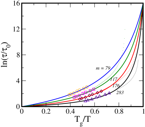
Figure 9: The Angell plot of the relaxation data. Also shown in the figure by dashed lines the corresponding power law fit predicted from the MCT ${\sim}(T-T_{c})^{a}$. The points shown are for $\eta_{0}$ =$.70$ (circles), $.69$ (squares), $.68$ (diamonds), $.67$ (triangles).

References

- (1) T.V. Ramakrishnan, and M. Yussouff, 1979, Phys. Rev. B 19, 2775.
-
(2)
J.-P. Hansen and I. R. McDonald,
Theory of Simple Liquids,
Elsevier Academic Press, 3rd ed. (2006). - (3) R. Evans, Adv. Phys. 28, 143 (1979).
- (4) P. Tarazona, Mol. Phys. 52, 871 (1984)
- (5) P.G. Wolynes, in Proceedings International Symposium on Frontiers in Science, eds. Frauenfelder, H., S. Chan, and DeBrunner, P.G. Wolynes, Am. Inst. Phys., pp 38, 1989.
- (6) C. A. Angell, Science 267, 1924 (1995)
- (7) R. Böhmer, and C. A. Angell, Phys. Rev. B 48, 5857 (1993).
- (8) S. P. Das, Phys. Rev. E 59, 3870 (1999)
- (9) S Srivastava, S. P. Das, Phys. Lett. A 286, 76 (2001)
- (10) J. S. Langer, Rep. Prog. Phys. 77, 042501 (2014).
- (11) A. Donev, F.H. Stillinger, S. Torquato, Phys. Rev. Lett. 96, 225502 (2006).
- (12) G. Adam and J. Gibbs, J. Chem. Phys. 43, 139 (1965)
- (13) S. Sengupta, S. Karmakar, C. Dasgupta, and S. Sastry, Phys. Rev. Lett. 109, 095705 (2012).
- (14) G.S. Fulcher J. Am. Ceram. Soc. 8, 339 (1925).
- (15) C. Kaur, U. Harbola, S. P. Das, J. of Chem. Phys. 123, 034501(2005).
- (16) Y. Singh, Phys. Reps. 207, 351 (1991).
- (17) H. Löwen, Phys. Reports B 237, 249 (1994).
-
(18)
S. P. Das, Statistical Physics of Liquids at Freezing and
Beyond,
Cambridge University Press, NewYork, (2011). - (19) S. P. Das, Rev. Mod. Phys. 76, 785 (2004).
- (20) D. R. Reichman and P. Charbonneau, J. Stat. Mech., P05013 (2005).
- (21) S. P. Das, J. of Chem. Phys. 98, 3328 (1993).
- (22) R. Ahluwalia, S. P. Das, Phys. Rev. E 57, 5771 (1998).
- (23) G. Biroli, and J-P Bouchaud, Euro Phys. Lett. 67, 21 (2004).
- (24) Y. Singh, J. P. Stoessel and P. G. Wolynes, 1985, Phys. Rev. Lett. 54, 1059.
- (25) C. Dasgupta, Europhys. Lett. 20, 131 (1992).
- (26) C. Kaur, and S. P. Das, Phys. Rev. Lett. 86, 2062 (2001).
-
(27)
P. Chaudhary, S. Karmakar, C. Dasgupta,
H.R. Krishnamurthy, A.K. Sood,
Phys. Rev. Lett. 95, 248301 (2005). - (28) B. S. Gupta, S. P. Das, and J-L Barrat, Phys. Rev. E 83, 041506 (2011).
- (29) L.M. Lust, O. T. Valls, and C. Dasgupta, Phys. Rev E. 48, 1787 (1993).
- (30) S.P. Das and G.F. Mazenko Phys. Rev. A 34, 2265 (1986).
- (31) J. Boon, and S. Yip, Molecular Hydrodynamics, Dover, New York, 1991.
- (32) D. Due, and A. D. J. Haymet, Jour. of Chem. Phys. 103, 2625 (1995).
- (33) D. Due, and D. Henderson, Jour. of Chem. Phys. 104, 6742 (1996).
- (34) M. Baus, and J.L. Colot, 1985, Mol. Phys. 55, 653.
- (35) S. Torquato, T.M. Tuskett, and P.G. Debenedetti, Phys. Rev. Lett. 84, 2064 (2000).
- (36) Löwen, J. Phys. C 2, 8477 (1990).
- (37) J. D. Bernal, Proc. R. Soc. London, Ser. A 280, 299 (1964).
- (38) Charles Bennett, J. Appl. Phys. 43, 2727 (1972).
- (39) D. Turnbull and J.C. Fisher, J. Chem. Phys. 17, 71 (1949).
- (40) R. Böhmer, and C. A. Angell, Phys. Rev. B 45, 10091 (1992).
- (41) A. R. Denton, and N. W. Ashcroft, Phys. Rev. A 39, 4701 (1989).
- (42) C. Kaur, S. P. Das, Phys. Rev. E 65, 026123(2002).
- (43) K. Kim, and T. Munakata, Phys. Rev. E, 68, 021502 (2003).