Electromagnetic vs. Lense-Thirring alignment of black hole accretion discs

Abstract

Accretion discs and black holes (BHs) have angular momenta that are generally misaligned with respect to each other, which can lead to warps in the discs and bends in any jets produced. We consider a disc that is misaligned at large radii and torqued by Lense-Thirring (LT) precession and a Blandford-Znajek (BZ) jet torque. We consider a variety of disc states that include radiatively inefficient thick discs, radiatively efficient thin discs, and super-Eddington accretion discs. The magnetic field strength of the BZ jet is chosen as either from standard equipartition arguments or from magnetically arrested disc (MAD) simulations. We show that standard thin accretion discs can reach spin-disc alignment out to large radii long before LT would play a role, as caused by the slow infall time that gives even a weak BZ jet time to align the disc. We show that geometrically thick radiatively inefficient discs and super-Eddington discs in the MAD state reach disc-spin alignment near the black hole when density profiles are shallow as in magnetohydrodynamical simulations, while the BZ jet aligns discs with steep density profiles (as in advection-dominated accretion flows) with the BH spin out to larger radii. Our results imply that the BZ jet torque should affect the cosmological evolution of BH spin magnitude and direction, BH spin measurements in active galactic nuclei and X-ray binaries, and the interpretations for Event Horizon Telescope observations of discs or jets in strong-field gravity regimes.

1 Introduction

Jets are ubiquitous in the Universe. While their formation mechanisms are still unclear, the required components appear to be a magnetic field, rotation, and accretion. In the case of black holes (BHs), the accretion is usually expected to take the form of a Keplerian disc with an angular momentum axis defined by the rotation of the disc material. The angular momentum of the source of disc matter, however, is capable of being arbitrarily misaligned with respect to the BH spin axis. Because BH jets are so prevalent, either the initial rotation of the matter is not important to jet formation, or the matter is torqued in some way to align with the angular momentum vector of the black hole. The gravitational potential of a rotating black hole is not spherically symmetric, so a different orientation of the disc could also have a significant effect on emergent radiation, affecting BH spin measurements (Kulkarni et al., 2011; McClintock et al., 2014), jet orientation (McKinney et al., 2013), and timing features in light curves (Ingram et al., 2009; Dexter & Fragile, 2013). Hence, determining whether (and to what degree) discs align by the action of BH spin is important.

There are a few processes through which material is torqued: 1) the exchange of angular momentum between neighbouring rings of material, a process called the accretion torque; 2) the Lense-Thirring effect, which is due to the dragging of spacetime by a rotating black hole combined with viscous forces (Lense & Thirring, 1918); and 3) a Blandford & Znajek (1977) (hereafter BZ) jet that is aligned with the rotation of the black hole near the black hole, but misaligned at larger radii by it trying to push on a misaligned disc (McKinney et al., 2013).

A study into magnetic alignment, corresponding to the third process, was performed by King & Lasota (1977) (hereafter KL, see also King et al. 2005), who concluded that either the inflow timescale was shorter than the alignment timescale, or the accretion rate was so low that the source could not be observed in the first place. Their negative result hinged on the assumptions that 1) the maximum magnetic field strength was limited by weak turbulent eddies in the disc; 2) the disc is rather small in radial extent with a relatively short inflow time; and 3) the disc followed the Shakura-Sunyaev density profile generalised by Novikov & Thorne (1973) (hereafter NT).

Since KL’s study on magnetic alignment, several disc models have been proposed, such as geometrically thick radiatively inefficient accretion flows (RIAFs) as the advection dominated accretion flow (ADAF) model (Narayan & Yi, 1994, 1995). The ADAF model has a steeper density profile than the NT solution, so a BH jet can more easily torque material at larger radii. The nature of the magnetic field can also be quite different, such as in the magnetically arrested disc (MAD) model (Narayan et al., 2003). In the MAD model, the magnetic field builds up near the black hole, until the magnetic tension is high enough that it balances inward forces due to the massive accretion flow. The magnetic field strengths attained are higher than previously considered, which means that magnetic alignment may yet actually be an efficient method of aligning the disc. Lastly, astrophysical discs can extend to tens of thousands of gravitational radii, where the inflow time becomes quite long and allows for the BZ jet torque to cumulate.

In this paper, we investigate how a disc aligns due to the Lense-Thirring and BZ jet torques by computing the disc shape from angular momentum conservation. We will demonstrate that disc alignment can occur for a variety of accretion rates, BH masses, and magnetic field strengths.

In Section 2 we will describe the equations we use to compare the different processes. In section 3 we will discuss the different accretion systems and disc models we will use. In Section 4 we will show the alignment of the different disc models and for a variety of systems such as Sgr A^∗ and GRS 1915+105. In Section 5 we will discuss the results, and in section 6 we will present our conclusions.

2 Method

In this section, we will obtain our equations of motion, give a description of the different scalings, and derive the external torques.

2.1 Equations of Motion

We start with the general relativistic magnetohydrodynamic (GRMHD) equations of motion, given by energy-momentum conservation:

$$\nabla_{\mu}(T^{\mu}_{\nu})=G_{\nu},$$ (1)

for an ideal stress-energy tensor $T^{\mu}_{\nu}=(\rho+p_{\mathrm{g}}+u_{\mathrm{g}}+b^{2})u^{\mu}u_{\nu}+\delta^{\mu}_{\nu}p_{\mathrm{tot}}-b^{\mu}b_{\nu}$ (given in terms of a coordinate basis), where we assume the induction equation controls the evolution of the magnetic field. The source term $G_{\nu}$ includes any disc cooling or external torques on the gas. After the usual height-integration and sticking to an orthonormal vector basis, one obtains for the $\phi$ equation of motion:

$$\frac{1}{r}\partial_{r}(r^{2}\Sigma v^{r}v^{\phi})=\tau_{\mathrm{acc}},$$ (2)

where $\Sigma=\int_{\theta}\rho r\,\mathrm{d}\theta=2\rho H$ and $\tau_{\mathrm{acc}}$ is the accretion torque per unit area that includes all magnetic and viscous terms that drive accretion and angular momentum transport (Frank et al., 2002). The height-integrated angular momentum per unit area is given by $\tilde{L}=r\Sigma v^{\phi}$, so that one can write the $\phi$ equation of motion as just

$$\frac{1}{r}\partial_{r}(rv^{r}\tilde{L})=\tau_{\mathrm{acc}}.$$ (3)

The equation in vector form for all components that is valid in the small-angle approximation is

$$\frac{1}{r}\partial_{r}(rv^{r}\vec{\tilde{L}})=\vec{\tau},$$ (4)

where $\tau$ is the total vector torque per unit area that includes the accretion torque and any other external torques (i.e. Lense-Thirring, Blandford-Znajek jet, etc.).

Figure 1: Schematic of the model used showing a slice through one side of the disc that has the most geometric misalignment with respect to the black hole. The disc is assumed to be non-axisymmetrically warped with no substantial twist. The disc starts out at an outer radius with an outer position angle $\theta_{\mathrm{out}}$ compared to the plane at $\theta=0$ of the black hole spin vector $j$. The accretion disc has angular momentum $L_{\mathrm{out}}$ and accretion is mediated by the accretion torque ($\tau_{\mathrm{acc}}$), which is always parallel to the angular momentum vector. At some radius ($R_{\mathrm{out}}$), the Blandford-Znajek ($\tau_{\mathrm{BZ}}$) and Lense-Thirring torque ($\tau_{\mathrm{LT}}$) start changing the direction of the angular momentum vector, and thereby the shape of the disc. The electromagnetic torque lies along the surface of the disc, while the Lense-Thirring torque points along the black hole spin vector plane for maximal alignment by forces driven by viscous action on Lense-Thirring precession torques. We calculate the magnitude and direction of the angular momentum ($L$), and hence the position angle ($\theta$) and the disc angle ($\theta_{\mathrm{disc}}$) of the disc (solid line) from the torques. If the disc has aligned to within a certain small angle relative to the initial angle $\theta_{\mathrm{out}}$, then we consider alignment effectively complete at that radius ($R_{\mathrm{in}}$).

2.2 Setup

Fig. 1 shows the general setup of our problem of a warped disc produced by torques that act to align an outer disc that is misaligned with respect to the BH spin axis. We assume the external torques all act to re-align the disc and do not cause twisting, precession, or breaking. So, the angular momentum vector of the disc reorients towards the BH spin axis without any twist. Then, there are only two angular momentum components to consider and so only two equations of motion to consider (i.e. the vector parallel to the BH spin axis and that perpendicular to the spin axis).

We assume small misalignments, so that the vector component for the misaligned angular momentum of $|\tilde{L}|\sin(\theta)$ is the required lowest-order term, meaning any dependence upon $\theta$ within the full tilted disc solution for $\Sigma$, $v^{r}$, or $v^{\phi}$ can be neglected as being a higher-order correction. Here $\theta$ is the angle away from the equatorial plane, and toward the $z$ axis is positive $\theta$. Similarly, for the aligned angular momentum of $|\tilde{L}|\cos(\theta)$, the perturbed disc solution would only be higher-order in $\theta$ and can be neglected for small tilts. This means that we can assume the radial profiles of $\Sigma$, $v^{r}$, and $v^{\phi}$ correspond to the original (e.g.) NT, ADAF, or untilted simulation profiles. This is why we do not have to consider the rest-mass or energy equations of motion.

The assumption of small tilt angles also means the radial direction and path length are approximately equal to the true disc direction and true disc path length, so we do not need to distinguish (say) $\vec{r}$ from $\vec{l}$, which would be the actual vector position of the disc. This means $v^{r}$ is a sufficiently accurate velocity along the disc path.

We calculate the magnitude of the angular momentum per unit area $\tilde{L}$ at some outer radius $R_{\mathrm{out}}$ at angle $\theta_{\mathrm{out}}$ and decompose it into an aligned component $L_{\parallel}=|\tilde{L}|\cos(\theta)$, parallel to the spin vector of the black hole, and a misaligned component $L_{\perp}=|\tilde{L}|\sin(\theta)$, pointing perpendicular to this direction. So, we have starting values $L_{\mathrm{out}\parallel}=|\tilde{L}|\cos(\theta_{\mathrm{out}})$ and $L_{\mathrm{out}\perp}=|\tilde{L}|\sin(\theta_{\mathrm{out}})$ at an outer radius $R_{\mathrm{out}}$ and outer disc position angle $\theta_{\mathrm{out}}$, where the starting values use $|\tilde{L}|$ from the untilted disc model. We use Eq. (4) to decompose the angular momenta into parallel and perpendicular components, giving:

$$\tau_{\mathrm{tot}\parallel} = \frac{1}{r}\partial_{r}(rv^{r}\tilde{L}_{\parallel}),$$ (5)

$$\tau_{\mathrm{tot}\perp} = \frac{1}{r}\partial_{r}(rv^{r}\tilde{L}_{\perp}).$$ (6)

We solve these torque equations discretely for new values of $\tilde{L}_{\parallel}$ and $\tilde{L}_{\perp}$ (giving $\theta$) for a radial step size $\Delta R\propto-R$, while the new disc angle $\theta_{\mathrm{disc}}$ is obtained from the difference in positions of the disc:

$$\halign to=0.0pt{\relax\global\advance\@IEEEeqncolcnt by 1\relax\begingroup\csname @IEEEeqnarraycolPREr\endcsname#\relax\relax\relax\relax\relax\relax\relax\relax\relax\relax\csname @IEEEeqnarraycolPOSTr\endcsname\relax\relax\relax\relax\relax\relax\relax\relax\relax\relax\endgroup&\relax\global\advance\@IEEEeqncolcnt by 1\relax\begingroup\csname @IEEEeqnarraycolPREC\endcsname#\relax\relax\relax\relax\relax\relax\relax\relax\relax\relax\csname @IEEEeqnarraycolPOSTC\endcsname\relax\relax\relax\relax\relax\relax\relax\relax\relax\relax\endgroup&\relax\global\advance\@IEEEeqncolcnt by 1\relax\begingroup\csname @IEEEeqnarraycolPREl\endcsname#\relax\relax\relax\relax\relax\relax\relax\relax\relax\relax\csname @IEEEeqnarraycolPOSTl\endcsname\relax\relax\relax\relax\relax\relax\relax\relax\relax\relax\endgroup&\global\advance\@IEEEeqncolcnt by 1\relax\bgroup#\egroup&\global\advance\@IEEEeqncolcnt by 1\relax\hbox to\z@\bgroup\hss#\egroup\cr\hfil$\displaystyle R_{n+1} $&\hfil$\displaystyle{}= {}$\hfil&$\displaystyle R_{n} + \Delta R,$\hfil&{{}\vrule width=0.0pt,height=0.0pt,depth=0.0pt}&0.0pt{\hss(7)}\cr\penalty 100\vskip 3.0pt\vskip 0.0pt\cr\hfil$\displaystyle\theta_{n+1} $&\hfil$\displaystyle{}= {}$\hfil&$\displaystyle\arctan(-L_{\perp}/ L_{\parallel}),$\hfil&{{}\vrule width=0.0pt,height=0.0pt,depth=0.0pt}&0.0pt{\hss(8)}\cr\penalty 100\vskip 3.0pt\vskip 0.0pt\cr\hfil$\displaystyle\theta_{\mathrm{disc}, n+1} $&\hfil$\displaystyle{}={}$\hfil&$\displaystyle\arctan\left[ \frac{R_{n+1} \sin(\theta_{n+1}) - R_{n} \sin(\theta_{n})}{R_{n+1} \cos(\theta_{n+1}) - R_{n} \cos(\theta_{n})} \right], $\hfil&{\vrule width=0.0pt,height=0.0pt,depth=0.0pt}&0.0pt{\hss(9)}\cr}$$

which after the first step no longer requires information from the untilted disc model for $\Sigma$ or $v_{\phi}$ – only $v^{r}$ is still required. In our small-angle approximation, the parallel torque equation just becomes an equation that ensures the accretion torque drives the correct behavior for the total angular momentum. The perpendicular torque equation contains all information about the actual angle, so in principle it can be solved for $\theta$ directly by plugging in the approximation that $\tilde{L}_{\perp}\approx|\tilde{L}|\sin(\theta)$ for all radii using the original untilted disc model value of $|\tilde{L}|$. We choose a slightly different but same-order accuracy approach, by evolving $\tilde{L}_{\parallel}$ and $\tilde{L}_{\perp}$ independently from each torque equation to obtain $\theta$ as in Eq. (2.2). This results in a total $\tilde{L}$ not identical with the untilted disc model value, but that is consistent with our small-angle approximation and the higher-order error becomes negligible for small $\theta$. We use at least ten steps per decade in radius, and to ensure accuracy we half the step size if the change in $\theta$ for any step is more than $\theta_{\mathrm{out}}/10$. We also check that our choice of initial angle leads to an $\tilde{L}$ similar to the untilted disc model value as must be true if we have chosen a sufficiently small angle so our approximations are valid.

2.3 Mass and Distance Scaling

Because we have systems with a wide range of masses, we will use the mass of the black hole in solar masses ($m=M/M_{\odot}$) as our mass scale, the corresponding gravitational radius as our length scale ($\bar{r}=r/r_{\mathrm{g}}$, with $r_{\mathrm{g}}=GM/c^{2}$), and the light crossing time as our time scale ($t_{\mathrm{g}}=GM/c^{3}$), with $G$ the gravitational constant, and $c$ the speed of light. We denote with a bar every variable that follows this scaling ($r\rightarrow\bar{r}$), and use small letters, or a different symbol for every variable that has an alternate scaling (i.e. total angular momentum of the BH as $J\rightarrow j$ that is the dimensionless BH spin, and magnetic flux $\Phi\rightarrow\Upsilon$ as the dimensionless magnetic flux). We scale the accretion rate to the Eddington accretion rate for a one solar mass black hole,

$$\dot{m}\equiv\dot{M}/\dot{M}_{\mathrm{Edd}}=\dot{M}_{\mathrm{BH}}/(\dot{M}_{\mathrm{Edd}\odot}m)\bar{r}^{s},$$ (10)

where $\dot{M}_{\mathrm{BH}}$ is the accretion rate at the horizon, $0\leq s\leq 1$ allowing for a wind if $s>0$, and where

$$\dot{M}_{\mathrm{Edd}\odot}=\frac{4\pi GM_{\odot}m_{\mathrm{p}}}{\eta c\sigma_{\mathrm{T}}}=\frac{1.40\times 10^{17}}{\eta}~{}\mathrm{g}~{}\mathrm{s}^{-1},$$ (11)

where $m_{\mathrm{p}}$ is the mass of a proton, $\eta$ is the arbitrarily-chosen nominal accretion efficiency of $\eta=0.1$, and $\sigma_{\mathrm{T}}$ is the Thomson cross section. We normalise the spin to the mass of the black hole, $j=\frac{c}{GM_{\odot}^{2}}m^{-2}J$. The dimensionless surface density is given by:

$$\bar{\Sigma}=\frac{G^{2}M_{\odot}}{c^{4}}m\Sigma,$$ (12)

and the dimensionless torque per unit area is:

$$\halign to=0.0pt{\relax\global\advance\@IEEEeqncolcnt by 1\relax\begingroup\csname @IEEEeqnarraycolPREr\endcsname#\relax\relax\relax\relax\relax\relax\relax\relax\relax\relax\csname @IEEEeqnarraycolPOSTr\endcsname\relax\relax\relax\relax\relax\relax\relax\relax\relax\relax\endgroup&\relax\global\advance\@IEEEeqncolcnt by 1\relax\begingroup\csname @IEEEeqnarraycolPREC\endcsname#\relax\relax\relax\relax\relax\relax\relax\relax\relax\relax\csname @IEEEeqnarraycolPOSTC\endcsname\relax\relax\relax\relax\relax\relax\relax\relax\relax\relax\endgroup&\relax\global\advance\@IEEEeqncolcnt by 1\relax\begingroup\csname @IEEEeqnarraycolPREl\endcsname#\relax\relax\relax\relax\relax\relax\relax\relax\relax\relax\csname @IEEEeqnarraycolPOSTl\endcsname\relax\relax\relax\relax\relax\relax\relax\relax\relax\relax\endgroup&\global\advance\@IEEEeqncolcnt by 1\relax\bgroup#\egroup&\global\advance\@IEEEeqncolcnt by 1\relax\hbox to\z@\bgroup\hss#\egroup\cr\hfil$\displaystyle\bar{\tau} $&\hfil$\displaystyle{}= {}$\hfil&$\displaystyle\frac{G^{2} M_{\odot}}{c^{6}} m \tau= 1.22 \times 10^{-44} m \tau. $\hfil&{\vrule width=0.0pt,height=0.0pt,depth=0.0pt}&0.0pt{\hss(13)}\cr}$$

2.4 Lense-Thirring Torque

The dragging of spacetime by a rotating black hole aligns material via the Lense-Thirring (LT) effect (Lense & Thirring, 1918). The LT effect inevitably leads to precession of the disc, but neighbouring rings can exchange angular momentum through viscosity, allowing alignment of the disc. Although this effect is only efficient very close to the black hole, the torque can also propagate outward via viscous forces, a process known as the Bardeen-Petterson effect (Bardeen & Petterson, 1975), which is commonly invoked as a method to align accretion discs with the spin of the black hole.

We assume the LT torque does not cause substantial twisting, so that twist angles are much smaller than the assumed small tilt angles. We also assume the disc does not break, as can occur for large tilt angles (Nixon & King, 2012). Lastly, we assume the disc does not precess, but we check our solutions for when precession is likely to occur (i.e. $\alpha>H/R$ for viscosity parameter $\alpha$ and height-to-radius ratio of $H/R$). In such cases when LT dominates alignment and $\alpha\gtrsim H/R$, we check if the BZ jet torque would have led to alignment anyway without the LT torque. We neglect apsidal precession, which could lead to additional effects.

The LT precession torque is given by

$$\tau_{\mathrm{LT}}\approx|\boldsymbol{\Omega}_{\mathrm{LT}}\times\boldsymbol{\tilde{L}}|\approx\Omega_{\mathrm{LT}}\tilde{L}\sin(\theta),$$ (14)

where $\Omega_{\mathrm{LT}}=2j/r^{3}$ describes the frame-dragging. For a general disc model, we assume a scaled Keplerian motion, so that the rotational velocity per unit speed of light is given by

$$\beta_{\phi}=\beta_{0}\bar{r}^{-1/2}=v_{\phi}/c.$$ (15)

So the dimensionless form of the LT torque is given by

$$\bar{\tau}_{\mathrm{LT}}\approx 2j\bar{\Sigma}\beta_{0}\sin(\theta)\bar{r}^{-5/2}.$$ (16)

Nominally some viscous process acts to redistribute the precession torque that could cause alignment in some cases. We assume the LT precession torque is re-directed by viscous interaction between differential precession as to maximally align the disc. This means that the LT torque magnitude is taken as the precession torque, but the direction is taken as that which maximally aligns the disc:

$$\tau_{\mathrm{LT},\parallel} \approx 0,$$ (17)

$$\tau_{\mathrm{LT},\perp} \approx \Omega_{\mathrm{LT}}\tilde{L}\sin(\theta).$$ (18)

This is generally not the case, but the final solution does not depend upon the LT torque direction being exactly along the perpendicular direction, and instead it could have been oriented perpendicular to the accretion torque or oriented along the disc like the electromagnetic torque. To lowest order in $\theta$, these all give the same resulting torque and behavior for $\tilde{L}$.

Our goal is to conservatively estimate whether the competing BZ jet torque can dominate any effect by LT. By choosing the maximal LT alignment effect, we give the LT torque the best chance to dominate the BZ jet torque physics. If our results show this conservative choice still leads to the BZ jet dominating the LT alignment, then our result of BZ dominance is robust to any weaker LT effect. Given the current significant uncertainty in how (or whether) the LT and other general relativistic effects lead to alignment, we take this simplifying approach in order to make restrictive statements about strength or physics involved in LT leading to alignment. If LT ends up causing less alignment, precession, or breaking, this only weakens the role of LT in aligning the disc and allows the BZ jet to more generally dominate.

2.5 Blandford-Znajek Jet Torque

If the electromagnetic (EM) jet is aligned with the rotation of the black hole, it can push on one side of a misaligned disc (McKinney et al., 2013). The torque described by KL was derived assuming vacuum conditions, so there is no spin-down or torque when the field is aligned with the black hole spin axis. However, Blandford & Znajek (1977) showed that even if the field is aligned with the BH spin axis, the BH will release angular momentum. In general, any orientation of the magnetic field will produce torques in the surrounding disc when the jet satisfies the conditions for force-free or magnetohydrodynamics (MHD). A BZ jet contains a constant magnetic flux and rotates at a constant field line rotation frequency along field lines (and individual field lines rotate at similar frequencies to order unity). For small spins, the spin axis does not necessarily control the jet direction even near the BH, while for larger spins the jet direction near the BH is dominated by the spin axis (McKinney et al., 2013). We assume the regime where the spin magnitude is large enough to have the jet aligned with the BH near the BH, although arbitrary angles applicable to small spins could be considered.

The BZ jet torque on the disc is due to the magnetic field draping the surface of the disc and pushing into the disc surface with a magnetic pressure. KL found that the torque along the azimuthal direction (into the plane in Fig. 1) vanishes, so there is no precessing torque. So the BZ jet torque has components

$$G_{\mathrm{BZ}\parallel} = |G_{\mathrm{BZ}}|\sin(\theta_{\mathrm{disc}}),$$ (19)

$$G_{\mathrm{BZ}\perp} = |G_{\mathrm{BZ}}|\cos(\theta_{\mathrm{disc}}),$$ (20)

$$G_{\mathrm{BZ}-y} = 0,$$ (21)

where KL found $|G_{\mathrm{BZ}}|\propto\sin(\theta)$. One could set $\theta_{\mathrm{disc}}\to\theta$ and our results are not substantially changed. We obtain the net torque per unit area $|\tau_{\mathrm{BZ}}|=|G_{\mathrm{BZ}}|/A$ for some area $A$ from $|G_{\mathrm{BZ}}|/A=|\vec{r}\times\Delta\vec{F}|/A=r(|\Delta F|/A)\cos(\theta-\theta_{\mathrm{disc}})$. The net force vanishes for zero tilt due to the jet pushing on the disc from above and below equally, while when the tilt is finite then the jet pushes down more on one side than the other. So $\Delta F\approx|F|\sin(\theta)$ for a one-sided force $|F|$, which gives

$$|G_{\mathrm{BZ}}|\approx r(|F|/A)\sin(\theta)\cos(\theta-\theta_{\mathrm{disc}}).$$ (22)

As the field rotates, the field could lag in shape and not follow the disc surface, which could introduce order unity changes to our force difference $\Delta F$. The one-sided force per unit area $|F|/A$ is due to the magnetic pressure $p_{b}$ of the jet pushing on the disc orthogonal to the disc surface. This gives that the net torque per unit area of the jet pushing down on the disc is

$$\tau_{\mathrm{BZ}\parallel} \approx rp_{b}\sin(\theta)\cos(\theta-\theta_{\mathrm{disc}})\sin(\theta_{\mathrm{disc}}),$$ (23)

$$\tau_{\mathrm{BZ}\perp} \approx rp_{b}\sin(\theta)\cos(\theta-\theta_{\mathrm{disc}})\cos(\theta_{\mathrm{disc}}),$$ (24)

which is consistent with KL’s torque direction and magnitude in the limit they considered where $\theta_{\mathrm{disc}}\to\theta$. The magnetic pressure is $p_{b}=b^{2}/(8\pi)$ (for $b$ in Gaussian units), $b^{\mu}=\frac{1}{2}\epsilon^{\mu\nu\kappa\lambda}u_{\nu}F_{\lambda\kappa}$ is the magnetic field 4-vector, $\epsilon$ is the Levi-Civita tensor, $u$ is the 4-velocity, and $F$ is the electromagnetic tensor (Gammie et al., 2003; McKinney, 2006a). In flat space-time, $b^{2}=\frac{B^{2}+(u\cdot B)^{2}}{\gamma^{2}}$. At large radii for a jet, $b^{2}\approx\frac{B_{\phi}^{2}}{\gamma^{2}}$, because the field becomes toroidal and the velocity becomes radial, while at small radii $b^{2}\approx B_{r}^{2}$ with a small angular velocity dominating the radial velocity. So, $(u\cdot B)\approx 0$ is generally small compared to the other term. The lab-frame magnetic field’s radial component $B_{r}$ is determined by the magnetic flux lines given by

$$\Phi_{G}(\theta)=(1/2)\int_{\theta\phi}r^{2}\sin(\theta)|B_{r}|\,\mathrm{d}\theta\,\mathrm{d}\phi,$$ (25)

with radial magnetic field $B_{r}$ in Gaussian units, and where $\Phi_{G}(\theta\approx\pi/2)\approx 2\pi r^{2-\nu}B_{r}$ with jet collimation parameter $0\leq\nu\lesssim 1$ described by the field shape

$$\Phi_{G}(\theta)\propto r^{\nu}[1-\sin(\theta)],$$ (26)

which is some constant $d$ for a field line of interest that closely hugs the disc surface with $\nu\approx 0$. The parameter $\nu$ could be derived by pressure-matching the jet magnetic pressure with the disc gas pressure for a given disc model (McKinney & Narayan, 2007a, b). In our case, we do not model the role of gas pressure, so the disc-jet interaction takes place as effectively having the magnetic field fill most of space for small tilt disc angles and small disc curvatures as if $\nu\approx 0$. We use a dimensionless magnetic flux passing through the BH horizon (at $r\approx r_{\mathrm{H}}$, the horizon radius) of

$$\Upsilon\approx 0.7\Phi_{G}[r=r_{\mathrm{H}}]/\sqrt{4\pi r_{\mathrm{g}}^{2}\dot{M}_{\mathrm{BH}}c}.$$ (27)

For force-free jets, the radial field is approximately related to the toroidal field by

$$B_{\phi}\approx B_{r}[r\Omega_{\mathrm{F}}\cos(\theta)]/c,$$ (28)

(Narayan et al., 2007), for field line angular frequency of rotation $\omega_{\mathrm{F}}=r_{\mathrm{g}}\Omega_{\mathrm{F}}/c\approx j/(4r_{\mathrm{H}})$, where the last approximation comes from the Blandford-Znajek split monopole valid at high $j$ (Blandford & Znajek, 1977; Tchekhovskoy et al., 2010a; Tchekhovskoy & McKinney, 2012; Tchekhovskoy et al., 2012). Thick discs could restrict some energy outflow and lead to a more rapid change in power as a function of $j$ (McKinney, 2005), but the total power output is the same at high $j$.

For an MHD jet, the behaviour of $B_{\phi}$ can be derived from energy conservation via the definition of $\mu$ that is the energy flux per unit rest-mass flux related to the conversion of electromagnetic to kinetic energy. This gives that

$$B_{\phi}\approx B_{\phi,\mathrm{fp}}\left(\frac{\gamma-\mu}{\gamma_{\mathrm{fp}}-\mu}\right)\left(\frac{r_{\mathrm{fp}}\Omega_{\mathrm{F},\mathrm{fp}}}{r\Omega_{\mathrm{F}}}\right),$$ (29)

so that for given foot point values ($B_{\phi,\mathrm{fp}}\approx B_{r,\mathrm{fp}}[r_{\mathrm{fp}}\Omega_{\mathrm{F},\mathrm{fp}}\cos(\theta_{\mathrm{fp}})]/c$, $r_{\mathrm{fp}}\approx r_{\mathrm{g}}$, $\gamma_{\mathrm{fp}}\approx 1$, $\Omega_{\mathrm{F},\mathrm{fp}}\approx\Omega_{\mathrm{F}}$ for our $\nu\approx 0$ case), we need $\gamma(r)$ to determine $B_{\phi}(r)$ (McKinney & Uzdensky, 2012). This MHD version of $B_{\phi}$ would not include any ram pressure or thermal pressure that would act to push the disc into alignment if the jet were aligned with the BH spin axis as it would be if the jet started as electromagnetic. The ram pressure is $\rho_{0}\gamma(\gamma-1)\approx B_{r}\gamma/\phi$ for conserved quantity $\phi\propto B_{r}/(\rho_{0}\gamma)$. The magnetic pressure dropping faster than $1/r^{2}$ once MHD acceleration occurs is therefore compensated by the ram pressure that still goes as $1/r^{2}$ for $B_{r}\propto r^{-2}$ with $\gamma$ going from $1\to\mu$. So we generally use Eq. (28) for $B_{\phi}$ to account for the total jet torque.

For the Lorentz factor’s radial dependence, we use the results from analytical calculations and simulations (Tchekhovskoy et al., 2008, 2009, 2010b; McKinney & Uzdensky, 2012). The Lorentz factor is given by

$$\frac{1}{\gamma}\approx\frac{1}{\gamma_{\mathrm{ff}}}+\frac{1}{\mu},$$ (30)

where $\gamma_{\mathrm{ff}}$ is the force-free Lorentz factor, and $\mu$ is the total energy flux per unit mass flux (and the upper limit of $\gamma$). Furthermore,

$$\frac{1}{\gamma_{\mathrm{ff}}^{2}}\approx\frac{1}{\gamma_{1}^{2}}+\frac{1}{\gamma_{2}^{2}},$$ (31)

where

$$\gamma_{1}\approx\sqrt{\gamma_{0}^{2}+(\Omega_{\mathrm{F}}R/c)^{2}-(\Omega_{\mathrm{F},\mathrm{fp}}R_{\mathrm{fp}}/c)^{2}},$$ (32)

describes the Lorentz factor first asymptotic regime due to the toroidal winding of the field lines, with $\Omega_{\mathrm{F},\mathrm{fp}}$ the field rotation frequency, and $R_{\mathrm{fp}}$ the radius at the footpoint of the field line. For curved field lines (i.e. $\nu>0$), the second asymptotic is given by

$$\gamma_{2,\nu}\approx\sqrt{CR_{\mathrm{c}}/R},$$ (33)

due to the collimation of the field lines, with $C\approx 3$ within factors of order unity, and $R_{\mathrm{c}}$ the poloidal radius of curvature of the field lines. In our approximation with $\nu\approx 0$, we have $R_{\mathrm{c}}\gg R$ so that $\gamma_{2}$ does not significantly change $\gamma_{\mathrm{ff}}$. In principle, $R_{c}$ can be computed as if the field followed the shape of the disc, and then $B_{r}$ would be computed by how the local magnetic flux changes in $\theta$. However, these effects are higher-order in tilt angle.

If the MHD jet is more conical (so has $\nu\sim 0$), the Lorentz factor behaves qualitatively differently with a Lorentz factor given by $\gamma=\gamma_{\mathrm{ff}}$, replacing the second asymptotic by the solution to the cubic equation

$$\gamma_{2,\nu=0}=C_{1}\left[\frac{(\mu-\gamma_{2,\nu=0})}{\sin^{2}(\theta_{c})}\ln{\left(1+C_{2}\frac{r\Omega_{\mathrm{F}}\sin(\theta_{c})}{c\gamma_{c}}\right)}\right]^{1/3},$$ (34)

where $C_{1}\approx 2$, $C_{2}\approx 0.4$, $\sin(\theta_{c})\sim\cos(\theta)\approx 1$ for $\theta$ away from the equator, and $\gamma_{c}\approx[\mu/\sin^{2}(\theta_{c})]^{1/3}\approx(\mu)^{1/3}$ (McKinney & Uzdensky, 2012). Because in this paper we are interested in $\nu\approx 0$, we set $\gamma_{2}=\gamma_{2,\nu=0}$. This forces the Lorentz factor to grow logarithmically with radius. This gives reasonable values of Lorentz factor as compared to GRMHD simulations of discs and jets that have $\gamma\sim 5$ by $r\sim 10^{3}~{}r_{\mathrm{g}}$ (McKinney, 2006b; McKinney & Blandford, 2009), e.g. for $\mu\sim 6$–$10$ at $r\sim 10^{3}~{}r_{\mathrm{g}}$–$10^{5}~{}r_{\mathrm{g}}$, this gives $\gamma_{2,\nu=0}\sim 4$–$8$.

2.6 Torque equations

For the given definitions of the internal and external torques, the parallel and perpendicular torques can be written as

$$\halign to=0.0pt{\relax\global\advance\@IEEEeqncolcnt by 1\relax\begingroup\csname @IEEEeqnarraycolPREr\endcsname#\relax\relax\relax\relax\relax\relax\relax\relax\relax\relax\csname @IEEEeqnarraycolPOSTr\endcsname\relax\relax\relax\relax\relax\relax\relax\relax\relax\relax\endgroup&\relax\global\advance\@IEEEeqncolcnt by 1\relax\begingroup\csname @IEEEeqnarraycolPREC\endcsname#\relax\relax\relax\relax\relax\relax\relax\relax\relax\relax\csname @IEEEeqnarraycolPOSTC\endcsname\relax\relax\relax\relax\relax\relax\relax\relax\relax\relax\endgroup&\relax\global\advance\@IEEEeqncolcnt by 1\relax\begingroup\csname @IEEEeqnarraycolPREl\endcsname#\relax\relax\relax\relax\relax\relax\relax\relax\relax\relax\csname @IEEEeqnarraycolPOSTl\endcsname\relax\relax\relax\relax\relax\relax\relax\relax\relax\relax\endgroup&\global\advance\@IEEEeqncolcnt by 1\relax\bgroup#\egroup&\global\advance\@IEEEeqncolcnt by 1\relax\hbox to\z@\bgroup\hss#\egroup\cr\hfil$\displaystyle\tau_{\mathrm{tot}\parallel} $&\hfil$\displaystyle{}= {}$\hfil&$\displaystyle- \tau_{\mathrm{BZ}}\sin(\theta_{\mathrm{disc}}) + \tau_{\mathrm{acc}}\cos(\theta), $\hfil&{{}\vrule width=0.0pt,height=0.0pt,depth=0.0pt}&0.0pt{\hss(35)}\cr\penalty 100\vskip 3.0pt\vskip 0.0pt\cr\hfil$\displaystyle\tau_{\mathrm{tot}\perp} $&\hfil$\displaystyle{}= {}$\hfil&$\displaystyle\tau_{\mathrm{LT}}+ \tau_{\mathrm{BZ}}\cos(\theta_{\mathrm{disc}}) + \tau_{\mathrm{acc}}\sin(\theta) , $\hfil&{\vrule width=0.0pt,height=0.0pt,depth=0.0pt}&0.0pt{\hss(36)}\cr}$$

which are used in Eq. (5). As discussed above, to lowest-order in $\theta$, the torque equation involving $\tau_{\mathrm{tot}\perp}$ controls the evolution of $\theta(r)$ and slight changes in direction of the LT or BZ jet torque give the same result.

3 Accretion Systems

In this section, we discuss the types of disc systems we consider.

3.1 Magnetic Field

For disc models not based upon simulations, we use that model’s arguments for equipartition magnetic fields within the disc itself. To get the field on the BH that drives the jet, we assume the radial field strength in the disc is

$$B_{r}(r=r_{\mathrm{H}})\sim\left(\frac{H}{R}\right)|B|(r=r_{\mathrm{H}}),$$ (37)

as expected when small-scale turbulent eddies of size $H$ in the disc set the scale of the radial field (Meier, 2001). This leads to a radial field much weaker for thin discs than if one assumed a dynamo existed that drove the toroidal field into a comparably strong poloidal field.

GRMHD simulations show that magnetic flux can build-up to a saturated value leading to the so-called magnetically-arrested disc (MAD). MAD simulations show that the BH magnetic flux magnitude is weakly dependent on BH spin but depends linearly on disc thickness as:

$$\Upsilon\approx 10\left(\frac{H/R}{0.3}\right),$$ (38)

(Tchekhovskoy et al., 2011; McKinney et al., 2012; Avara et al., 2015). Thin or thick non-MAD discs whose poloidal field is generated spontaneously reaches up to $\Upsilon\sim 3$ (Shafee et al., 2008; Penna et al., 2010; McKinney et al., 2012), which is typically stronger than that obtained from nominal equipartition arguments due to magnetic compression and lower plasma $\beta_{\mathrm{MHD}}\sim 1$ (i.e. gas to magnetic pressure ratio of order unity) near the BH horizon (Penna et al., 2010; McKinney et al., 2012).

3.2 Advection-Dominated Accretion Flow for the limits of Radiatively Inefficient Accretion Flow and Super-Eddington Accretion

At low accretion rates, the flow is too tenuous to radiate efficiently and becomes a RIAF. A classic model of a RIAF is the Advection-Dominated Accretion Flow (ADAF) with most of the internal energy being advected with the flow into the black hole before it can be radiated away or before it can be blown into a wind (Narayan & Yi, 1994, 1995). A typical RIAF disc, such as in Sgr A^∗ or M87, may extend out to $10^{4}~{}r_{\mathrm{g}}$ or $10^{6}~{}r_{\mathrm{g}}$.

The extreme ADAF case with ratio of specific heats $\Gamma=5/3$ has purely radial accretion not typical of what is found in simulations. To more closely connect with simulation results, we assume $\Gamma=1.63$, corresponding to $\beta_{\mathrm{MHD}}=P_{\mathrm{gas}}/P_{\mathrm{mag}}=5$ (Quataert & Narayan, 1999a). Furthermore we will assume the efficiency of advection $f=1$ (no radiative losses), and consequently $\epsilon^{\prime}=(5/3-\Gamma)/[f(\Gamma-1)]\approx 0.17$, $c_{1}=0.059$, $c_{2}=0.15$, $c_{3}=0.39$, which are the ratio of the radial velocity to the Keplerian rotational velocity, the ratio of the angular velocity to the Keplerian angular velocity, and the square root of the ratio of the sound speed to the Keplerian rotational velocity, respectively. Furthermore, $H/R=\sqrt{c_{3}}\approx 0.62$, and $\beta_{0}=c_{2}=0.15$. The surface density is given by:

$$\bar{\Sigma}=\left[\frac{G^{2}M_{\odot}}{c^{4}}m\right]\frac{\dot{M}}{2\pi rv_{r}}=\frac{G}{c^{3}}\frac{\dot{M}_{\mathrm{Edd}\odot}}{2\pi}c_{1}^{-1}m\dot{m}_{\mathrm{BH}}\bar{r}^{s-1/2}.$$ (39)

An ADAF wind can lead to less sub-Keplerian motion, for example $s=0.4$ gives $\beta_{0}\approx 0.53$ (Quataert & Narayan, 1999b). In order to estimate the magnetic field strength for the equipartition state near the BH for the jet magnetic field strength, we assume $\beta_{\mathrm{MHD}}=1$ seen in GRMHD simulations, which gives $\beta_{\mathrm{m}}=P_{\mathrm{gas}}/(P_{\mathrm{gas}}+P_{\mathrm{mag}})=0.5$ for $P_{\mathrm{rad}}=0$. To calculate the dimensionless magnetic flux on the black hole, we assume that the magnetic field, $B=\sqrt{2\dot{M}_{\mathrm{Edd}\odot}}\frac{c^{5/2}}{GM_{\odot}}m^{-1/2}\dot{m}^{1/2}\left(1-\beta_{\mathrm{m}}\right)^{1/2}\alpha^{-1/2}c_{1}^{-1/2}c_{3}^{1/4}\bar{r}^{3/4}$ gives the total field, and then we use Eq. (37) to obtain the radial component. This leads to a magnetic flux of $\Phi=2\pi r_{\mathrm{H}}^{2}|B_{r}|(r_{\mathrm{H}})$, and:

$$\Upsilon=\left(\frac{2\pi}{\dot{M}_{\mathrm{Edd}\odot}}\right)^{1/2}\frac{GM_{\odot}}{c^{5/2}}m^{1/2}\dot{m}^{-1/2}r_{\mathrm{H}}^{2}B_{r}(r_{\mathrm{H}}).$$ (40)

Otherwise, for a MAD RIAF, we use the simulation scaling of $\Upsilon$ as a function of $H/R$.

3.3 Novikov & Thorne disc

At higher accretion rates, the disc becomes geometrically thin as described by Novikov & Thorne (1973), a general relativistic extension to the disc model by Shakura & Sunyaev (1973). We include the relativistic corrections and use the surface density of the appropriate region based upon the opacity and gas or radiation dominance as in the original paper by NT. A typical BH X-ray binary disc extends out to $10^{5}~{}r_{\mathrm{g}}$ or $10^{6}~{}r_{\mathrm{g}}$ (e.g. Orosz et al. 2009).

To obtain the BH jet field strength for the equipartition magnetic field case, we calculate the maximum magnetic field strength at twice the innermost stable circular orbit (ISCO, which lies at $5~{}r_{\mathrm{g}}$ for $j=0.9$) and assume the field at this location is the same total strength as the strength over the horizon and then we use Eq. (37) to obtain the radial component. For the MAD state we use $H/R\approx 0.257L/L_{\mathrm{Edd}}$ corresponding to the maximum thickness near the BH that would trap the hole’s magnetic flux. So,

$$\Upsilon=10\left(\frac{0.257L/L_{\mathrm{Edd}}}{0.3}\right)=10\left(\frac{0.257\dot{m}}{0.3}\right)$$ (41)

Although it is possible to modify the Novikov & Thorne disc with a wind (Miller, 2015), we have set $s=0$ for this model.

3.4 Slim disc

In the high accretion rate limit, a reasonable analytical solution is the slim disc model, which at high enough rates just becomes the ADAF model for a $\Gamma=4/3$ gas – which is what we assume as our model in this limit as valid in the limit of a radiation-dominated flow. This gives $\epsilon^{\prime}=1$, $c_{1}=0.43$, $c_{2}=0.53$, $c_{3}=0.29$, and $H/R=\sqrt{c_{3}}\approx 0.53$, and $\beta_{0}=c_{2}=0.53$. The smaller $H/R$ ratio causes a reduced (electro-)magnetic torque, while the higher rotational velocity will increase the accretion and Lense-Thirring torque, when compared with the low luminosity case. A typical tidal disruption event (TDE) disc might extend out to $10^{3}~{}r_{\mathrm{g}}$ or $10^{6}~{}r_{\mathrm{g}}$ (Dai et al., 2015). We use the same magnetic field conditions for the jet magnetic field strength as the ADAF case.

3.5 GRMHD simulations

For a general radiatively inefficient accretion flow (RIAF) we use the results of numerical simulations. GRMHD simulations have a density profile $\rho\propto\bar{r}^{-0.7}$ and $v_{r}\sim\alpha(H/R)^{2}v_{\phi}$ for some total constant $\alpha(H/R)^{2}$ (McKinney & Gammie, 2004; Penna et al., 2010; McKinney et al., 2012), giving a surface density profile:

$$\bar{\Sigma}=\left[\frac{G^{2}M_{\odot}}{c^{4}}m\right]2\rho H=\frac{G}{c^{3}}\frac{\dot{M}_{\mathrm{Edd}\odot}}{2\pi}\bar{r}_{+}^{-2}m\dot{m}_{\mathrm{BH}}\bar{r}^{0.3}.$$ (42)

Note that one cannot infer the outflow parameter $s$ in $\dot{M}\propto r^{s}$ from this density scaling, e.g. convective dominated accretion flows (CDAFs) have shallow density profiles compared to ADAFs even without unbound outflows. However, this is not required as we only need the density and $H$ scaling to get our required $\Sigma$. In practice, GRMHD simulations do not reach very large radii, but such density scalings are seen in non-general relativistic simulations that extend to large radii where a power-law fit is quite reliable (Pen et al., 2003; Pang et al., 2011).

The $\phi$-velocity scaling seen in GRMHD simulations is quite Keplerian for non-MAD discs, while for MAD simulations a slightly steeper or shallower scaling may occur (McKinney et al., 2012), which could slightly change our results. For the non-MAD case, we use $\beta_{0}=1$, while for the MAD state we take $\beta_{0}=0.5$ as valid for $H/R\approx 0.4$ (McKinney et al., 2012) that is applicable to RIAFs according to such simulations.

The BH jet magnetic field is set by the simulation condition of $\Upsilon\sim 3$ for equipartition and set using the simulation scaling of $\Upsilon$ with $H/R$ for a MAD.

3.6 Overall Disc Model

We branch between different disc solutions based upon $\dot{m}$ given the estimated matching between disc theory and observations. For $\dot{m}=L/L_{\mathrm{Edd}}<10^{-3}$ we assume the system to be in a low accretion RIAF state, using the ADAF state as detailed in section 3.2 or the GRMHD simulation state as detailed in section 3.5. For $10^{-3}<\dot{m}<10^{-2}$ we linearly interpolate the relevant disc variables ($\beta_{0}$, $\beta_{R}$, $\bar{\Sigma}$, and $\Upsilon_{\mathrm{BH}}$), between the low accretion RIAF and a Novikov & Thorne disc described in section 3.3. For $10^{-2}<\dot{m}<1$, we use the Novikov & Thorne solution only. For $1<\dot{m}<30$ we linearly interpolate between the Novikov & Thorne disc and the high accretion slim disc (in RIAF limit) as described in Section 3.4. For $30<\dot{m}$ we use the high accretion slim disc solution.

4 Results

We assume the following values in all default cases, unless otherwise specified: $\alpha=0.1$, a moderately high spin of $j=0.9$, $s=0$, $\mu=3$ for stellar-mass black holes and $\mu=10$ for supermassive black holes, $\theta_{\mathrm{out}}=5^{\circ}$, and $r_{\mathrm{out}}=10^{5}~{}r_{\mathrm{g}}$. By default, we assume the RIAF is modelled by GRMHD simulation results.

Fig. 2 shows our results for a broad set of mass accretion rates for a black hole mass of $m=15$ consistent with GRS 1915+105 (a typical stellar-mass black hole) in the non-MAD and MAD states. Alignment is effective (either by the LT or BZ jet torque) in the NT state because of the relatively slow radial velocity for thin discs. This gives the LT or BZ jet torque time to align the disc as material accretes inwards. Naturally, the LT torque is only clearly dominant for the thin disc case where the magnetic field is weak due to the drop in magnetic flux as $H/R$ drops. However, even in the NT state the thickness is not too small for $\dot{m}\gtrsim 0.3$, beyond which the BZ jet torque dominates alignment. In either case, the NT disc is aligned out to $r\sim 10^{3}~{}r_{\mathrm{g}}$.

Alignment is not so effective in the RIAF state assuming the GRMHD simulation scaling of density, but still alignment occurs within $r\sim 10~{}r_{\mathrm{g}}$ as primarily due to the radial component of the magnetic field. This is despite the relatively larger value of $\Upsilon$, compared to the NT disc case, due to the thick disc at $H/R\approx 0.4$. Even in the equipartition magnetic field case, the BZ jet torque tends to dominate the torques, but alignment is dominated by LT torques – so precession might occur instead for the equipartition magnetic field case.

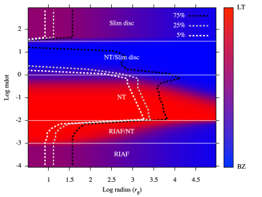
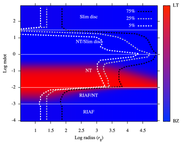
Figure 2: Overview of the dominant torque for a range of radii and accretion rates for our overall disc model for the equipartition magnetic field model (left panel) and for the MAD magnetic field model (right panel) for GRS 1915+105. Blue corresponds to dominance by the BZ torque, while red corresponds to dominance by LT precession torques, with blends of colour in-between. The rapid transitions at some $\dot{m}$ are due to the interpolation between the RIAF and NT discs. This is caused by the surface density dropping monotonically with radius in a RIAF, while it rises quickly in the NT case. The dashed lines show when the angle of the disc has reached 75%, 25%, and 5% of the original angle. Our results are independent of the initial angle for small angles. The NT disc is aligned effectively by LT torques at lower mass accretion rates, except if the field strength reaches MAD levels where the NT disc is aligned by the BZ torques before the LT torques can operate. The RIAF models are only aligned with $r\sim 10~{}r_{\mathrm{g}}$ due to the rapid infall time compared to the time it takes to modify the angular momentum by the LT or BZ torques.

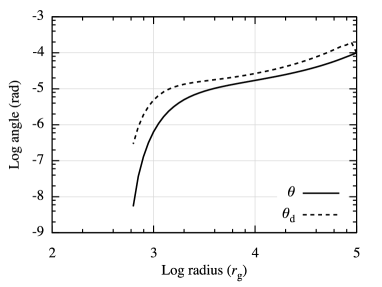
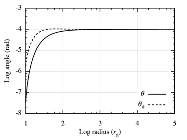
Figure 3: Solution from torque equations for disc position angle $\theta$ and disc orientation angle $\theta_{\mathrm{disc}}$ for the case of GRS 1915+105 in the high-soft state where $L/L_{\mathrm{Edd}}=\dot{M}/\dot{M}_{\mathrm{Edd}}\sim 0.3$ (left panel) and Sgr A^∗ (right panel). We have chosen the MAD RIAF simulation case for Sgr A^∗ and chosen the MAD NT case for GRS 1915+105. In both cases, the disc extends out to $r_{\mathrm{out}}\sim 10^{5}~{}r_{\mathrm{g}}$, so we have chosen that as our outer disc radius. In the standard thin disc case, at high enough $\dot{m}\gtrsim 0.3$, the BZ jet torque dominates the LT torque and causes alignment out to $r\sim 10^{3}~{}r_{\mathrm{g}}$. For the case of Sgr A^∗, the alignment occurs much closer to the BH at $r\sim 10~{}r_{\mathrm{g}}$ due to the rapid infall time.

Fig. 3 shows the values of $\theta$ and $\theta_{\mathrm{disc}}$ for the case of Sgr A^∗ with $m\approx 4.5\times 10^{6}$, $\dot{m}\sim 1.5\times 10^{-6}$, and $\mu=10$ and for the case of GRS 1915+105 (in the high-soft state where $L/L_{\mathrm{Edd}}\sim 0.3$) with $m\approx 15$, $\dot{m}\sim 0.3$, and $\mu=3$. In both cases the magnetic field is assumed to be MAD. As indicated in Fig. 2 for $\dot{m}\lesssim 0.3$, close to the black hole the LT torque dominates, but for $\dot{m}\gtrsim 0.3$ the BZ jet torque dominates and causes alignment out to $r\sim 10^{3}~{}r_{\mathrm{g}}$ before the LT torque has a chance to operate. In the case of Sgr A^∗, the inflow time is more rapid than in the standard thin disc case, but the disc still aligns by the BZ jet torque by $r\sim 10~{}r_{\mathrm{g}}$ as consistent with GRMHD simulations of tilted discs around rotating black holes (McKinney et al., 2013).

4.1 LT versus BZ Jet Torque in Causing Alignment

In some cases, the LT torque can appear to dominate, but we have assumed a maximally aligning LT torque to test if the BZ jet torque still dominates alignment. We can also check the case when the LT torque is weak (e.g., due to the LT torque instead leading to precession) to see if the BZ jet torque alone is sufficient to lead to substantial alignment. If so, then even in those regions dominated by the LT torque, the BZ torque is sufficient regardless of the regime the LT torque operates in (i.e. diffusive versus wave-like).

We repeat the above analysis, but this time turn off the LT torque entirely. For the MAD case, we find that the BZ jet torque indeed leads to substantial alignment even in regions where the LT torque could dominate. For example, in the transition region between NT and slim disc regimes, the BZ torque alone is sufficient to align material out to thousands of gravitational radii.

This means that even if LT leads to precession once $H/R$ increases compared to $\alpha$ as $\dot{m}$ rises towards Eddington, the BZ torque can still align the disc out to large radii. So, the BZ torque can align the disc before the LT torque would have a chance to cause precession. In some cases, the intermediate regime occurs, where the BZ torque could lead to alignment, but at such radii the LT torque is already strong, in which case the disc could be partially precessing and partially aligning.

4.2 Dependence upon ADAF vs. GRMHD Simulations as RIAF Model

The RIAF model applies at very low or very high accretion rates. In our default model, we select the simulation results as most accurately portraying this regime. Here instead we consider the ADAF model as our RIAF model. We repeat the same analysis as for our default case, but consider how the RIAF regime changes.

Due to the steep density profile in the ADAF case, we find that the jet rapidly aligns the disc out near the starting radius. This is because there is effectively much less angular momentum at large radii compared to the default model. The ADAF case leads to most of the mass reaching the BH, leading to a maximally effective jet that can more readily affect the outer disc. In real discs, such as for Sgr A^∗, one expects the disc to transition to the Bondi inflow that itself will transition to the ambient medium outside the influence of the BH’s gravitational potential (e.g. Li et al. 2013).

The ADAF RIAF case is the only case where the results are also significantly affected by how we treat the jet as either force-free or MHD. In particular, we have only considered the electromagnetic contribution to any pressure by the jet on the disc. As electromagnetic energy is converted to kinetic energy in an MHD jet, the electromagnetic contribution drops as our MHD jet case describes. This leads to an ineffective electromagnetic pressure at large radii in the ADAF RIAF case. However, as described above, the total pressure is best modelled by the force-free case, so that the entire ADAF aligns out to large radius.

4.3 Dependence upon other model parameters

Here we consider the dependence on other model parameters, including the outer disc radius $r_{\mathrm{out}}$, total energy flux per unit rest-mass flux in the jet $\mu$, dimensionless BH spin $j$, rotation rate $\beta_{0}$, wind mass loss power-law index $s$, viscosity parameter $\alpha$, and magnetic collimation parameter $\nu$. In each case, we repeat the analysis for new parameters.

For discs starting at smaller radii down to $r=100~{}r_{\mathrm{g}}$, the LT torque plays a stronger role even for the RIAF regime. This suggests that for small discs, like those that may be present during some deep penetrating tidal disruption events, the disc may tend to precess more than align.

For $\mu=10$ (instead of our default $\mu=6$) or slightly higher values of $\mu=20$, the results are similar with the expected less effective magnetic pressure that scales as $1/\gamma^{2}$ where $\gamma\to\mu$ at large radii. For smaller discs the change in $\mu$ leads to less dramatic effects because $\gamma$ has not reached terminal values near $\mu$.

A smaller BH spin $j$ leads to a weaker jet as expected because the magnetic pressure roughly scales as $j^{2}$. Because the LT torque scales as only $j$, this means eventually at small enough $j$ the LT torque dominates (whether or not alignment occurs) and the BZ torque plays no role as expected.

The rotation rate factor $\beta_{0}$ is typically fixed for each disc model type, but smaller values lead to weaker LT torques and allow the BZ torque to more easily dominate and lead to alignment because the disc has less angular momentum for the same jet magnetic pressure (that does not directly depend upon the disc rotation rate). MADs tend to be more sub-Keplerian, so the stronger field leads to a stronger jet that even more easily aligns the more slowly-rotating material.

The mass-loss-rate power-law index $s$ that enters $\dot{M}\propto r^{s}$ allows a shallower density profile, which makes the inner jet less effective at aligning material present at fixed large radii. The simulation scalings used already effectively include a wind, and there is still aligning at least within the region near the BH.

A smaller viscosity parameter of $\alpha=0.01$ leads to a slower inflow rate, giving the LT torque or BZ jet torque more time to align the material out to larger radii. In this case, the BZ jet torque aligns the RIAF simulation material out to $r\sim 100~{}r_{\mathrm{g}}$ instead of just $r\sim 10~{}r_{\mathrm{g}}$. The NT region is aligned by LT torques out to $r\sim 10^{4}~{}r_{\mathrm{g}}$ instead of just $r\sim 10^{3}~{}r_{\mathrm{g}}$.

The magnetic collimation parameter $\nu$ is chosen as $\nu\approx 0$ as we do not include the disc pressure matching to the jet pressure. Disc vertical stratification and pressure can force $\nu\approx 0.7$ (McKinney & Narayan, 2007a), leading to a stronger magnetic pressure for any given radius. This would lead to a much stronger BZ torque, however a compensating factor is that collimating jets also become causally disconnected from the disc and itself (Porth & Komissarov, 2015). The balance of these effects is left for future work.

5 Discussion

The Lense-Thirring torque has a steep dependence with radius, so it can more readily dominate the BZ torque at small radii. At larger radii, the BZ jet torque can readily dominate. If the BZ torque leads to substantial alignment at large radii, then the LT torque has no chance to operate and cannot align or lead to precession. Whether alignment occurs depends upon the disc model: NT models tend to align by LT and other models tend to align by the BZ jet torque.

The BZ torque depends on the magnetic flux, and since large scale magnetic fields can be more easily supported by thick discs (Meier, 2001; Narayan et al., 2003; McKinney et al., 2012), it is not surprising that for a thick disc these torques are more effective than for thin discs. For this reason in the thin Novikov & Thorne disc, the Lense-Thirring and accretion torque dominate, but for even higher accretion rates, which cause the disc to become thicker, the (electro-)magnetic torque becomes more dominant.

The LT torque depends on the density distribution, which can change its radial profile. In the case of the inner region of a Novikov & Thorne disc, this dependency gives it a slope as flat as the accretion torque, making it the strongest throughout that region. When a density distribution with a negative radial dependence is used, the Lense-Thirring torque quickly becomes negligible, sometimes not even dominating at all. If most accretion happens at (super-)Eddington rates, the disc will be thick, and the Bardeen-Petterson effect will cause precession instead of alignment, also decreasing the importance of the Lense-Thirring torque. For these two reasons the Bardeen-Petterson effect can become negligible in these systems, a hypothesis supported by recent numerical simulations (Fragile et al., 2007; Morales Teixeira et al., 2014; Zhuravlev et al., 2014, and references therein). As a result we may need to look to other torquing mechanisms to align the disc in astrophysical systems.

The Blandford-Znajek torque estimates in this paper assume a simple monopolar field geometry ($\nu\approx 0$), while collimating jets have a magnetic torque that drops off more slowly, and such geometries may be more effective than we have assumed. On the other hand, the jet can become ballistic before the Blandford-Znajek torque is completely effective. These effects need to be modelled with detailed simulations. We have included the equations for general values of $\nu$ in this paper.

Our approach to computing the disc shape and including the torques is quite simplified, but improves the one in King & Lasota (1977). They compared the timescale of accretion to the timescale of magnetic alignment for a disc that is rigid over an extended range of radii. In our case, the disc shape is computed by the inclusion of advection terms that account for the timescale of accretion versus alignment at each radius. We allow for stronger MAD-strength magnetic fields, and we allow the disc to extend to physically reasonable larger radii where the timescale for inflow becomes long enough for the BZ torque to become more effective.

We have performed simple calculations of the disc shape due to aligning torques caused by the BH spin axis being different than the disc angular momentum axis. Our approach is rougher in handling the Lense-Thirring torques than other analytical works (Zhuravlev & Ivanov, 2011), but no other work has considered the competing effects of Lense-Thirring and Blandford-Znajek jet torques. We treat the Blandford-Znajek torque fairly accurately. Naturally, prior analytical work is also unable to treat the magnetic field within the disc accurately except as a viscosity.

Our calculation for the Lense-Thirring aligning torque is rough, but we chose the torque to be maximally aligning with the goal of testing whether the BZ jet torque could still dominate alignment. Any other missing physics that leads to precession, breaking, or oscillation by Lense-Thirring would only weaken its ability to align before the BZ jet aligns the disc. In that sense, the calculation conservatively determines where the BZ jet dominates alignment.

We have also taken a simple approach because simulations are expensive and have yet to be self-consistent. That is, simulations have so-far been limited to using an effective viscosity instead of turbulent magnetic fields (Nelson & Papaloizou, 2000; Zhuravlev & Ivanov, 2011), tend to not resolve the MRI and consider relatively thick discs in full GR (Morales Teixeira et al., 2014), or approximate GR with relatively thick discs (Sorathia et al., 2013). We have also neglected apsidal precession, which could lead to additional external torques. While our calculations are rough, this has allowed us to scan a broader parameter space of possible disc models, black hole masses, accretion rates, and magnetic field types. And it has allowed us to consider the role of jet-induced alignment that otherwise requires expensive simulations (McKinney et al., 2013).

The simulations performed by McKinney et al. (2013) show alignment results reasonably consistent with our calculations, with the RIAFs in the MAD state effectively aligning near the BH. They estimated the BZ jet torque analytically as an internal torque with $\tau\sim rB_{r}B_{\phi}\sin(\theta)$ – which is only roughly a good approximation close to the black hole.

6 Conclusions

We have considered the competition between Lense-Thirring and Blandford-Znajek jet torques in driving alignment between the disc angular momentum vector and BH spin vector. We have studied a broad parameter space of possible disc models, black hole masses, accretion rates, and magnetic field types in order to determine the disc shape, what radius alignment occurs, and which torque dominates the alignment process.

In those regions where BZ jet alignment is effective at aligning the disc, Lense-Thirring becomes unimportant and ineffective because the material is already aligned by the BZ jet before Lense-Thirring operates. This also means that Lense-Thirring will be ineffective at other non-aligning processes like precession and disc breaking.

For BH X-ray binaries, state transitions show a variety of temporal and spectral features that are difficult to explain theoretically (McClintock & Remillard, 2006; Remillard & McClintock, 2006; McClintock et al., 2006). GRS 1915+105 is particularly prolific by exhibiting an array of complicated temporal features. Some of these temporal features occur when GRS 1915+105 is near the Eddington rate, which we find is where the MAD state can cause the BZ jet torque to align the material, while for slightly sub-Eddington rates the Lense-Thirring torque dominates and could cause some precession or alignment. A combination of precession by LT, alignment by LT and BZ torques, and quasi-periodic oscillations driven by the MAD state and a BZ jet (McKinney et al., 2012), and variations in the magnetic field (leading to different alignment and precessing torques) might interact to produce such a diverse set of temporal phenomena.

If accretion happens at (or above) Eddington rates, the cosmological evolution of black hole mass and spin may not be determined by the Bardeen-Petterson effect, but rather by (electro-)magnetic processes. The Blandford-Znajek torque can be a significant factor in a wide range of accretion rates relevant to cosmological large-scale structure simulations, so it should be taken into consideration.

The Event Horizon Telescope (EHT) focuses on the strong-field gravity regime within tens of gravitational radii, and polarisation is capable of probing the nature of the magnetic field there (Shcherbakov et al., 2012; Dexter et al., 2012; Johnson, 2015). Warps in the disc or bends in the jet near such scales could be revealed by changes in the polarised emission by different cancellations in the polarisation when the jet bends. Our results are consistent with the self-consistent GRMHD simulations by McKinney et al. (2013), who found disc alignment occurs within $r\sim 10~{}r_{\mathrm{g}}$. This is on the scale observed by the EHT, so one expects the warping of the disc or jet to manifest in EHT observations. Warps, oscillations, or precession could create observable timing features (Shcherbakov & McKinney, 2013). If warps are present out to large radii, this can affect Faraday rotation measures from discs and jets (Broderick & McKinney, 2010). High-energy emission from jets, as observed by Fermi, could have signatures of disc or jet warps (O’ Riordan et al., 2015).

The primary assumption made in this work is the small-angle approximation, but this has allowed us to investigate a broad space of disc models and parameters. The hope is this inspires self-consistent simulations that account for the competing roles between the Lense-Thirring and Blandford-Znajek jet torques when considering the alignment or breaking of discs. Simulations are now able to account for vertical stratification, winds, magnetic fields, and radiation, which removes the ambiguity of the transitions between disc models and can account directly for these competing effects (Sa̧dowski et al., 2014; McKinney et al., 2014; McKinney et al., 2015). Simulation models include much more physics than we have included, and can treat the regime where the magnetic field undergoes polarity inversions (Dexter et al., 2014), which might light up the jet to reveal the warped jet and disc. Simulations in the thin disc regime can be expensive, but our results show that even a study at moderate Eddington factors ($L/L_{\mathrm{Edd}}\sim 0.3$) might show interesting competition between these torques while being in an astrophysically relevant regime.

References

- Avara et al. (2015) Avara M. J., McKinney J. C., Reynolds C. S., 2015, ArXiv/1508.05323
- Bardeen & Petterson (1975) Bardeen J. M., Petterson J. A., 1975, ApJ, 195, L65
- Blandford & Znajek (1977) Blandford R. D., Znajek R. L., 1977, MNRAS, 179, 433
- Broderick & McKinney (2010) Broderick A. E., McKinney J. C., 2010, ApJ, 725, 750
- Dai et al. (2015) Dai L., McKinney J. C., Miller M. C., 2015, ApJ, 812, L39
- Dexter & Fragile (2013) Dexter J., Fragile P. C., 2013, MNRAS, 432, 2252
- Dexter et al. (2012) Dexter J., McKinney J. C., Agol E., 2012, MNRAS, 421, 1517
- Dexter et al. (2014) Dexter J., McKinney J. C., Markoff S., Tchekhovskoy A., 2014, MNRAS, 440, 2185
- Fragile et al. (2007) Fragile P. C., Blaes O. M., Anninos P., Salmonson J. D., 2007, ApJ, 668, 417
- Frank et al. (2002) Frank J., King A., Raine D. J., 2002, Accretion Power in Astrophysics: Third Edition. Cambridge University Press
- Gammie et al. (2003) Gammie C. F., McKinney J. C., Tóth G., 2003, ApJ, 589, 444
- Ingram et al. (2009) Ingram A., Done C., Fragile P. C., 2009, MNRAS, 397, L101
- Johnson (2015) Johnson M. D. e. a., 2015, Science, 350, 1242
- King & Lasota (1977) King A. R., Lasota J. P., 1977, A&A, 58, 175
- King et al. (2005) King A. R., Lubow S. H., Ogilvie G. I., Pringle J. E., 2005, MNRAS, 363, 49
- Kulkarni et al. (2011) Kulkarni A. K., Penna R. F., Shcherbakov R. V., Steiner J. F., Narayan R., Sä Dowski A., Zhu Y., McClintock J. E., Davis S. W., McKinney J. C., 2011, MNRAS, 414, 1183
- Lense & Thirring (1918) Lense J., Thirring H., 1918, Physikalische Zeitschrift, 19, 156
- Li et al. (2013) Li J., Ostriker J., Sunyaev R., 2013, ApJ, 767, 105
- McClintock et al. (2014) McClintock J. E., Narayan R., Steiner J. F., 2014, Space Science Reviews, 183, 295
- McClintock & Remillard (2006) McClintock J. E., Remillard R. A., 2006, Black hole binaries. pp 157–213
- McClintock et al. (2006) McClintock J. E., Shafee R., Narayan R., Remillard R. A., Davis S. W., Li L.-X., 2006, ApJ, 652, 518
- McKinney (2005) McKinney J. C., 2005, ApJ, 630, L5
- McKinney (2006a) McKinney J. C., 2006a, MNRAS, 367, 1797
- McKinney (2006b) McKinney J. C., 2006b, MNRAS, 368, 1561
- McKinney & Blandford (2009) McKinney J. C., Blandford R. D., 2009, MNRAS, 394, L126
- McKinney et al. (2015) McKinney J. C., Dai L., Avara M. J., 2015, MNRAS, 454, L6
- McKinney & Gammie (2004) McKinney J. C., Gammie C. F., 2004, ApJ, 611, 977
- McKinney & Narayan (2007a) McKinney J. C., Narayan R., 2007a, MNRAS, 375, 513
- McKinney & Narayan (2007b) McKinney J. C., Narayan R., 2007b, MNRAS, 375, 531
- McKinney et al. (2012) McKinney J. C., Tchekhovskoy A., Blandford R. D., 2012, MNRAS, 423, 3083
- McKinney et al. (2013) McKinney J. C., Tchekhovskoy A., Blandford R. D., 2013, Science, 339, 49
- McKinney et al. (2014) McKinney J. C., Tchekhovskoy A., Sadowski A., Narayan R., 2014, MNRAS, 441, 3177
- McKinney & Uzdensky (2012) McKinney J. C., Uzdensky D. A., 2012, MNRAS, 419, 573
- Meier (2001) Meier D. L., 2001, ApJ, 548, L9
- Miller (2015) Miller M. C., 2015, ApJ, 805, 83
- Morales Teixeira et al. (2014) Morales Teixeira D., Fragile P. C., Zhuravlev V. V., Ivanov P. B., 2014, ApJ, 796, 103
- Narayan et al. (2003) Narayan R., Igumenshchev I. V., Abramowicz M. A., 2003, PASJ, 55, L69
- Narayan et al. (2007) Narayan R., McKinney J. C., Farmer A. J., 2007, MNRAS, 375, 548
- Narayan & Yi (1994) Narayan R., Yi I., 1994, ApJ, 428, L13
- Narayan & Yi (1995) Narayan R., Yi I., 1995, ApJ, 444, 231
- Nelson & Papaloizou (2000) Nelson R. P., Papaloizou J. C. B., 2000, MNRAS, 315, 570
- Nixon & King (2012) Nixon C. J., King A. R., 2012, MNRAS, 421, 1201
- Novikov & Thorne (1973) Novikov I. D., Thorne K. S., 1973, in Dewitt C., Dewitt B. S., eds, Black Holes (Les Astres Occlus) Astrophysics of black holes.. pp 343–450
- O’ Riordan et al. (2015) O’ Riordan M., Pe’er A., McKinney J. C., 2015, ArXiv/1510.08860
- Orosz et al. (2009) Orosz J. A., Steeghs D., McClintock J. E., Torres M. A. P., Bochkov I., Gou L., Narayan R., Blaschak M., Levine A. M., Remillard R. A., Bailyn C. D., Dwyer M. M., Buxton M., 2009, ApJ, 697, 573
- Pang et al. (2011) Pang B., Pen U.-L., Matzner C. D., Green S. R., Liebendörfer M., 2011, MNRAS, 415, 1228
- Pen et al. (2003) Pen U.-L., Matzner C. D., Wong S., 2003, ApJ, 596, L207
- Penna et al. (2010) Penna R. F., McKinney J. C., Narayan R., Tchekhovskoy A., Shafee R., McClintock J. E., 2010, MNRAS, 408, 752
- Porth & Komissarov (2015) Porth O., Komissarov S. S., 2015, MNRAS, 452, 1089
- Quataert & Narayan (1999a) Quataert E., Narayan R., 1999a, ApJ, 516, 399
- Quataert & Narayan (1999b) Quataert E., Narayan R., 1999b, ApJ, 520, 298
- Remillard & McClintock (2006) Remillard R. A., McClintock J. E., 2006, ARA&A, 44, 49
- Sa̧dowski et al. (2014) Sa̧dowski A., Narayan R., McKinney J. C., Tchekhovskoy A., 2014, MNRAS, 439, 503
- Shafee et al. (2008) Shafee R., McKinney J. C., Narayan R., Tchekhovskoy A., Gammie C. F., McClintock J. E., 2008, ApJ, 687, L25
- Shakura & Sunyaev (1973) Shakura N. I., Sunyaev R. A., 1973, A&A, 24, 337
- Shcherbakov & McKinney (2013) Shcherbakov R. V., McKinney J. C., 2013, ApJ, 774, L22
- Shcherbakov et al. (2012) Shcherbakov R. V., Penna R. F., McKinney J. C., 2012, ApJ, 755, 133
- Sorathia et al. (2013) Sorathia K. A., Krolik J. H., Hawley J. F., 2013, ApJ, 777, 21
- Tchekhovskoy & McKinney (2012) Tchekhovskoy A., McKinney J. C., 2012, MNRAS, 423, L55
- Tchekhovskoy et al. (2008) Tchekhovskoy A., McKinney J. C., Narayan R., 2008, MNRAS, 388, 551
- Tchekhovskoy et al. (2009) Tchekhovskoy A., McKinney J. C., Narayan R., 2009, ApJ, 699, 1789
- Tchekhovskoy et al. (2012) Tchekhovskoy A., McKinney J. C., Narayan R., 2012, Journal of Physics Conference Series, 372, 012040
- Tchekhovskoy et al. (2010a) Tchekhovskoy A., Narayan R., McKinney J. C., 2010a, ApJ, 711, 50
- Tchekhovskoy et al. (2010b) Tchekhovskoy A., Narayan R., McKinney J. C., 2010b, New Astronomy, 15, 749