Microscopic nuclear structure models and methods : Chiral symmetry, Wobbling motion and $\gamma-$bands

Abstract

A systematic investigation of the nuclear observables related to the triaxial degree of freedom is presented using the multi-quasiparticle triaxial projected shell model (TPSM) approach. These properties correspond to the observation of $\gamma$-bands, chiral doublet bands and the wobbling mode. In the TPSM approach, $\gamma$-bands are built on each quasiparticle configuration and it is demonstrated that some observations in high-spin spectroscopy that have remained unresolved for quite some time could be explained by considering $\gamma$-bands based on two-quasiparticle configurations. It is shown in some Ce-, Nd- and Ge-isotopes that the two observed aligned or s-bands originate from the same intrinsic configuration with one of them as the $\gamma$-band based on a two-quasiparticle configuration. In the present work, we have also performed a detailed study of $\gamma$-bands observed up to the highest spin in Dysposium, Hafnium, Mercury and Uranium isotopes. Furthermore, several measurements related to chiral symmetry breaking and wobbling motion have been reported recently. These phenomena, which are possible only for triaxial nuclei, have been investigated using the TPSM approach. It is shown that doublet bands observed in lighter odd-odd Cs-isotopes can be considered as candidates for chiral symmetry breaking. Transverse wobbling motion recently observed in ¹³⁵Pr has also been investigated and it is shown that TPSM approach provides a reasonable description of the measured properties.

1 Introduction

Atomic nucleus is one of the most fascinating quantum many-body systems that depicts a rich variety of shapes and structures. At the same time, it is also one of the most challenging problems in physics to investigate theoretically. The number of particles is not too large as in condensed matter physics so that statistical tools become applicable and also it is not too small such that few-body techniques can be employed for nuclei across the periodic table. The phenomenal progress in understanding the properties of nuclei has been achieved using phenomenological models and methods. These phenomenological models are primarily based on empirical observations and have played a pivotal role in unraveling the intrinsic structures of atomic nuclei [1, 2, 3, 4, 5].

The pioneering work of Bohr, Mottelson and Rainwater laid the foundation of the phenomenological models in nuclear physics. It was demonstrated that properties of atomic nuclei can be elucidated by considering rotational, vibrational and single-particle motion as three basic degrees of freedom and led to the development of the collective model in sixties and seventies [6, 7]. This model is even being used today with the parameters determined through microscopic approaches rather than following the empirical route.

The nuclear physics research is going through a renaissance with the state-of-the-art tools and techniques being developed to probe the wealth of nuclear properties. The availability of the leadership computing facilities has made it possible to apply Ab-initio methods to lighter mass region with remarkable success. On the other hand, the density functional approach is now widely used to explore the ground-state properties all across the nuclear landscape [8, 9, 10]. In recent years, the progress achieved in applying these modern tools is quite remarkable and it is expected that it would be possible to apply these techniques to investigate a broad spectrum of nuclear properties all across the nuclear periodic table [11, 12] in a forseeable future. However, at the moment, these models have limitations and cannot be employed to investigate, for instance, the rich-band structures observed in deformed nuclei.

In the absence of a fully microscopic theory, semi-microscopic models have been developed to study the properties of band structures in medium and heavy mass nuclei. In this class of models, the triaxial projected shell model (TPSM) approach has been demonstrated to correlate the high-spin data of well deformed and transitional data with remarkable success [13]. The purpose of the present work is to provide an overview of the recent applications of the TPSM approach to a wide range of nuclear properties [14, 15, 16, 17, 18, 19, 20, 21, 21, 22, 23, 24, 25, 26, 27, 28]. We also report new results on the observation of $\gamma$ bands based on excited configurations. Furthermore, we shall present a systematic investigation of $\gamma-$bands observed up to the highest spin in Dysposium, Hafnium, Mercury and Uranium isotopes. The manuscript is organised in the following manner. In the next section, a few details of the TPSM approach are provided and some technical aspects of the model are included in the appendix. In section 3, the results of the calculations for $\gamma$-, chiral- and wobbling- bands are displayed and discussed. Finally, the work presented in this manuscript is summarized and concluded in section 4.

2 Outline of the Triaxial Projected Shell Model Approach

The basic philosophy of the TPSM approach is similar to the spherical shell model model (SSM) with the only difference that deformed basis are employed for diagonalizing the shell model Hamiltonian rather than the spherical one. The deformed basis are constructed by solving the triaxial Nilsson potential with optimum quadrupole deformation parameters of $\epsilon$ and $\epsilon^{\prime}$. In principle, the deformed basis can be constructed with arbitrary deformation parameters, however, the basis are constructed with expected or known deformation parameters (so called optimum) for a given system under consideration. These deformation values lead to an accurate Fermi surface and it is possible to choose a minimal subset of the basis states around the Fermi surface for a realistic description of a given system. The Nilsson basis states are then transformed to the quasiparticle space using the simple Bardeen-Cooper-Schriefer (BCS) ansatz for treating the pairing interaction.

As the deformed basis are defined in the intrinsic frame of reference and don’t have well defined angular-momentum, in the second stage these basis are projected onto states with well defined angular-momentum using the angular-momentum projection technique [29, 30, 31]. The three dimensional angular-momentum projection operator is given by

$$\hat{P}^{I}_{MK}=\frac{2I+1}{8\pi^{2}}\int d\Omega\,D^{I}_{MK}(\Omega)\,\hat{R}(\Omega),$$ (1)

with the rotation operator

$$\hat{R}(\Omega)=e^{-i\alpha\hat{J}_{z}}e^{-i\beta\hat{J}_{y}}e^{-i\gamma\hat{J}_{z}}.$$ (2)

Here, ${}^{\prime\prime}\Omega^{\prime\prime}$ represents a set of Euler angles ($\alpha,\gamma=[0,2\pi],\,\beta=[0,\pi]$) and the $\hat{J}^{\prime}s$ are angular-momentum operators. The projected basis states considered in the present work for the even-even system are composed of vacuum, two-proton, two-neutron and two-proton plus two-neutron configurations, i.e.,

$$\{\hat{P}^{I}_{MK}\left|\Phi\right>,~{}\hat{P}^{I}_{MK}~{}a^{\dagger}_{p_{1}}a^{\dagger}_{p_{2}}\left|\Phi\right>,~{}\hat{P}^{I}_{MK}~{}a^{\dagger}_{n_{1}}a^{\dagger}_{n_{2}}\left|\Phi\right>,$$

$$~{}\hat{P}^{I}_{MK}~{}a^{\dagger}_{p_{1}}a^{\dagger}_{p_{2}}a^{\dagger}_{n_{1}}a^{\dagger}_{n_{2}}\left|\Phi\right>\},$$ (3)

where $\left|\Phi\right>$ in (3) represents the triaxial qp vacuum state. The above basis space used for the even-even system is sufficient to study nuclei up to second band crossing region and in the rare-earth region this means approximately up to spin, I=24 $\hbar$. For odd-proton (neutron) systems, the basis space is composed of one-quasiproton (quasineutron) and two-quasineutrons (quasiprotons). In the case of odd-odd nuclei, the basis space is simply one-quasiproton coupled to one- quasineutron.

The advantage of the TPSM approach as compared to the other approaches, for instance the cranking approach, is that not only the yrast band but also the rich excited band structures can be investigated. As a matter of fact, the major focus of the present work is to study the $\gamma$-bands which form the first excited band in many transitional nuclei. The Nilsson triaxial quasiparticle states don’t have well defined projection along the symmetry axis, $\Omega$ and are a superposition of these states. For instance, the triaxial self-conjugate vacuum state is a superposition of K = 0, 2, 4,…states - only even-states are possible due to symmetry requirement [32]. For the symmetry operator, $\hat{S}=e^{-\imath\pi\hat{J}_{z}}$, we have

$$\hat{P}^{I}_{MK}\,|\,\Phi\!>\,=\hat{P}^{I}_{MK}\hat{S}^{\dagger}\hat{\,}|\,\Phi\!>\,=e^{\imath\pi(K-\kappa)}\hat{P}^{I}_{MK}\,|\,\Phi\!>\,,$$ (4)

where, $\hat{S}\,|\,\Phi\!>\,=e^{-\imath\pi\kappa}\,|\,\Phi\!>\,$, and $\kappa$ characterizes the intrinsic states. For the self-conjugate vacuum state $\kappa=0$ and, therefore, it follows from the above equation that only $K=$ even, values are permitted for this state. For 2-qp states, the possible values for $K$-quantum number are both even and odd depending on the structure of the qp state. For the 2-qp state formed from the combination of the normal and the time-reversed states, $\kappa=0$ and again only $K=$ even values are permitted. For the combination of the two normal states, $\kappa=1$, and only $K=$ odd states are allowed.

The projected states for a given configuration that constitute a rotational band are obtained by specifying the corresponding K-value in the angular-momentum projection operator. The projected states from K = 0, 2 and 4 correspond to ground-, $\gamma-$ and $\gamma\gamma-$bands, respectively. As stated earlier, for two-quasiparticle states, both even- and odd-K values are permitted depending on the signature of the two quasiparticle states. In this description, the aligning states that cross the ground-state band and lead to upbend or backbend phenomenon have K = 1. The projection from the same quasiparticle intrinsic state with K = 3 is the $\gamma$-band built on these two quasiparticle state. The $\gamma$-bands built on the two-quasiparticle states shall form one of the major focal issues of the present work and shall be discussed in detail in the next section.

In the third and the final stage of the TPSM analysis, the projected basis are employed to diagonalize the shell model Hamiltonian. The model Hamiltonian consists of pairing and quadrupole-quadrupole interaction terms, i.e.,

$$\hat{H}=\hat{H}_{0} - {1\over 2}\chi\sum_{\mu}\hat{Q}^{\dagger}_{\mu}\hat{Q}_{\mu}-G_{M}\hat{P}^{\dagger}\hat{P}$$ (5)

$$- G_{Q}\sum_{\mu}\hat{P}^{\dagger}_{\mu}\hat{P}_{\mu}.$$

In the above equation, $\hat{H}_{0}$ is the spherical single-particle Nilsson Hamiltonian [33]. The parameters of the Nilsson potential are fitted to a broad range of nuclear properties and is quite appropriate to employ it as a mean-field potential. The QQ-force strength, $\chi$, in Eq. (5) is related to the quadrupole deformation $\epsilon$ as a result of the self-consistent HFB condition and the relation is given by [34]:

$$\chi_{\tau\tau^{\prime}}={{{2\over 3}\epsilon\hbar\omega_{\tau}\hbar\omega_{\tau^{\prime}}}\over{\hbar\omega_{n}\left<\hat{Q}_{0}\right>_{n}+\hbar\omega_{p}\left<\hat{Q}_{0}\right>_{p}}},$$ (6)

where $\omega_{\tau}=\omega_{0}a_{\tau}$, with $\hbar\omega_{0}=41.4678A^{-{1\over 3}}$ MeV, and the isospin-dependence factor $a_{\tau}$ is defined as

$$a_{\tau}=\left[1\pm{{N-Z}\over A}\right]^{1\over 3},$$

with $+$ $(-)$ for $\tau=$ neutron (proton). The harmonic oscillation parameter is given by $b^{2}_{\tau}=b^{2}_{0}/a_{\tau}$ with $b^{2}_{0}=\hbar/{(m\omega_{0})}=A^{1\over 3}$ fm². The monopole pairing strength $G_{M}$ (in MeV) is of the standard form

$$G_{M}={{G_{1}-G_{2}{{N-Z}\over A}}\over A}~{}{\rm for~{}neutrons,}~{}~{}~{}~{}$$ (7)

$$G_{M}={G_{1}\over A}~{}{\rm for~{}protons.}$$

In the present calculation, we choose $G_{1}$ and $G_{2}$ such that the observed odd-even mass difference is reproduced in the mass region. The values $G_{1}$ and $G_{2}$ vary depending on the mass region and shall be mentioned in the discussion of the results. The above choice of $G_{M}$ is appropriate for the single-particle space employed in the model, where three major shells are used for each type of nucleon. The quadrupole pairing strength $G_{Q}$ is considered to be proportional to $G_{M}$ and the proportionality constant being fixed as 0.18. These interaction strengths are consistent with those used in our earlier studies [14, 15, 16, 17, 19, 32, 34, 35, 36, 37, 38, 39].

It is shown in the appendix that the projection formalism outlined above can be transformed into a diagonalization problem following the Hill-Wheeler prescription. The Hamiltonian in Eq. (5) is diagonalized using the projected basis of Eq. (3). The obtained wavefunction can be written as

$$\psi^{\sigma}_{IM}=\sum_{K,\kappa}a^{\sigma}_{\kappa}\hat{P}^{I}_{MK}|~{}\Phi_{\kappa}\!>\,.$$ (8)

Here, the index $\sigma$ labels the states with same angular momentum and $\kappa$ the basis states. In Eq. (8), $a^{\sigma}_{\kappa}$ are the amplitudes of the basis states $\kappa$. These wavefunction are used to calculate the electromagnetic transition probabilities. The reduced electric quadrupole transition probability $B(E2)$ from an initial state $(\sigma_{i},I_{i})$ to a final state $(\sigma_{f},I_{f})$ is given by [40]

$$B(E2,I_{i}\rightarrow I_{f})={\frac{e^{2}}{2I_{i}+1}}|\,<\!\sigma_{f},I_{f}||\hat{Q}_{2}||\sigma_{i},I_{i}\!>\,|^{2}.$$ (9)

As in our earlier publications [20, 21, 22, 23, 24], we have used the effective charges of 1.6e for protons and 0.6e for neutrons. The reduced magnetic dipole transition probability $B(M1)$ is computed through

$$B(M1,I_{i}\rightarrow I_{f})={\frac{\mu_{N}^{2}}{2I_{i}+1}}|\,<\!\sigma_{f},I_{f}||\hat{\mathcal{M}}_{1}||\sigma_{i},I_{i}\!>\,|^{2},$$ (10)

where the magnetic dipole operator is defined as

$$\hat{\mathcal{M}}_{1}^{\tau}=g_{l}^{\tau}\hat{j}^{\tau}+(g_{s}^{\tau}-g_{l}^{\tau})\hat{s}^{\tau}.$$ (11)

Here, $\tau$ is either $\nu$ or $\pi$, and $g_{l}$ and $g_{s}$ are the orbital and the spin gyromagnetic factors, respectively. In the calculations we use for $g_{l}$ the free values and for $g_{s}$ the free values damped by a 0.85 factor, i.e.,

$$g_{l}^{\pi}=1,~{}~{}~{}g_{l}^{\nu}=0,~{}~{}~{}$$

$$g_{s}^{\pi}=5.586\times 0.85,$$

$$g_{s}^{\nu}=-3.826\times 0.85.$$ (12)

The reduced matrix element of an operator $\hat{\mathcal{O}}$ ($\hat{\mathcal{O}}$ is either $\hat{Q}$ or $\hat{\mathcal{M}}$) can be expressed as

$$\,<\!\sigma_{f},I_{f}||\hat{\mathcal{O}}_{L}||\sigma_{i},I_{i}\!>\,$$

$$= \sum_{\kappa_{i},\kappa_{f}}{f_{I_{i}\kappa_{i}}^{\sigma_{i}}}{f_{I_{f}\kappa_{f}}^{\sigma_{f}}}\sum_{M_{i},M_{f},M}(-)^{I_{f}-M_{f}}$$

$$\times \left(\begin{array}[]{ccc}I_{f}&L&I_{i}\\ -M_{f}&M&M_{i}\end{array}\right)$$

$$\times \,<\!\phi_{\kappa_{f}}|{\hat{P}^{I_{f}}}_{K_{\kappa_{f}}M_{f}}\hat{\mathcal{O}}_{LM}\hat{P}^{I_{i}}_{K_{\kappa_{i}}M_{i}}|\phi_{\kappa_{i}}\!>\,$$

$$= 2\sum_{\kappa_{i},\kappa_{f}}{a_{I_{i}\kappa_{i}}^{\sigma_{i}}}{a_{I_{f}\kappa_{f}}^{\sigma_{f}}}\sum_{M^{\prime},M^{\prime\prime}}(-)^{I_{f}-K_{\kappa_{f}}}{(2I_{f}+1)}^{-1}$$

$$\times \left(\begin{array}[]{ccc}I_{f}&L&I_{i}\\ -M_{\kappa_{f}}&M^{\prime}&M^{\prime\prime}\end{array}\right)~{}\int d\Omega\,D_{M^{\prime\prime}\kappa_{\kappa_{i}}}(\Omega)$$ (18)

$$\times \,<\!\Phi_{\kappa_{f}}|\hat{\mathcal{O}}_{LM^{\prime}}\hat{R}(\Omega)|\Phi_{\kappa_{i}}\!>\,.$$ (19)

In the above expression, the symbol $(~{}~{}~{}~{}~{}~{})$ denotes a 3j-coefficient.

Table 1: Axial and non-axial quadrupole deformation values $\epsilon$ and $\epsilon^{\prime}$ employed in the TPSM calculation for Ce and Nd isotopes. Axial deformations $\epsilon$ have been considered from [41] and nonaxial values are chosen in such a way that band heads of the $\gamma-$ bands are reproduced.

A	$\epsilon$	$\epsilon^{\prime}$	$\gamma$
132Ce	0.183	0.100	29
134Ce	0.150	0.100	34
134Nd	0.200	0.120	31
136Nd	0.158	0.110	35
138Nd	0.170	0.110	33

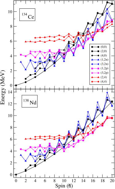
Figure 1: (Color online) Band diagrams for ¹³⁴Ce and ¹³⁸Nd isotopes as representative examples. The labels ($K$,n-qp) indicate the $K$-value and the quasiparticle character of the configuration, for instance, $(3,2n)$ corresponds to the 2n-aligned $\gamma$-band built on 2n-aligned state.

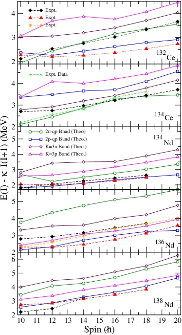
Figure 2: (Color online) Theoretical bands with the dominant component from (1, 2n), (1, 2p), (3, 2n), and (3, 2p). Only spin range from I = 10 to 20 is shown for which these bands are low in energy. Available data in ^132,134Ce and ^134,136,138Nd are compared with the calculated results. Data has been taken from Refs. [75, 76, 77, 78, 79].

3 Results and Discussions

In the past few years, TPSM approach has been used quite extensively to shed light on some of the outstanding issues related to the triaxility in atomic nuclei and in the present section we shall provide a brief overview of these investigations and some new results obtained recently shall also be presented and discussed. This section is divided into subsections, discussing various aspects and implications on the presence of triaxial deformations in atomic nuclei.

3.1 Observation of the $\gamma$-bands based on two-quasiparticle states

$\gamma$-bands are observed in most of the transitional nuclei all across the nuclear periodic table and have been studied using various theoretical approaches and methods [42, 43, 44, 45, 46, 47, 48, 49, 50, 51, 52, 53, 54, 55, 56, 57]. In phenomenological models, these bands are interpreted as emerging due to vibrational motion in the $\gamma$ degree of freedom of the nuclear deformation [58, 59, 60, 61, 62, 63, 64, 65, 66, 67, 68, 69, 70].

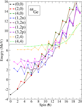
Figure 3: (Color online) Band diagram for ⁶⁸Ge isotope. The labels ($K$,n-qp) indicate the $K$-value and the quasiparticle character of the configuration, for instance, $(3,2n)$ corresponds to the 2n-aligned $\gamma$-band built on 2n-aligned state K=1 quasiparticle configuration.

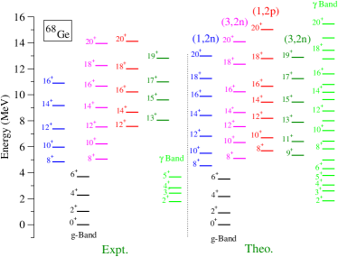
Figure 4: (Color online) Comparison of the measured energy levels of ⁶⁸Ge nucleus and the results of TPSM calculations. Data has been taken from Refs. [80].

In the microscopic TPSM approach, $\gamma$-band structure results from the projection of the K = 2 component of the triaxial vacuum state. $\gamma$-bands are also possible based on the multi-quasiparticle triaxial states apart from the vacuum configuration and have not been studied as most of the models consider vacuum configuration only. The basis of TPSM approach has been enlarged to include multi-quasiparticle states and it is now possible to investigate $\gamma$-bands built on quasiparticle structures. It is demonstrated in the present work that excited band structures observed in some nuclei that have remained abstruse for many years are, in fact, the $\gamma$-bands based on two-quasiparticle states. In the following, we shall provide results of the TPSM calculations for ^132,134Ce-, ^134,136,138Nd- and ⁶⁸Ge-isotopes where some excited bands are proposed as the $\gamma$-bands based on two-quasiparticle configurations.

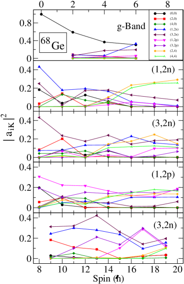
Figure 5: (Color online) Probability of various projected K-configurations in the wavefunctions of the observed bands for ⁶⁸Ge. For clarity, only the lowest projected K-configurations in the wavefunctions of bands are shown and in the numerical calculations, projection has been performed from more than forty intrinsic states.

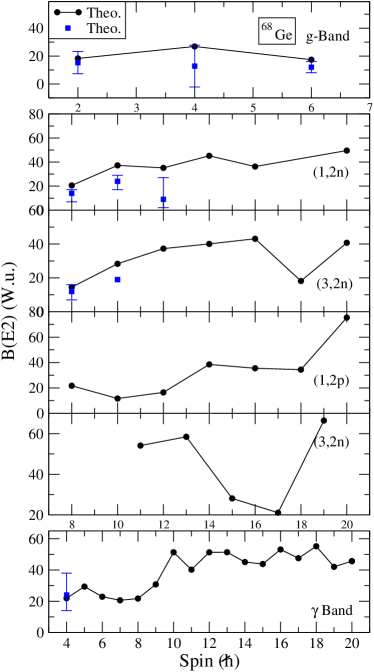
Figure 6: (Color online) Comparison of the calculated B(E2) (W.u.) with available experimental data for ⁶⁸Ge. Data has been taken from Refs. [81].

In ¹³⁴Ce, the ground-state band is observed to fork into two s-bands and the band heads of both these bands are known to have negative g-factors, indicating that both of them have neutron configurations [71]. In many rotational nuclei, the ground-state band is crossed by a two quasiparticle state having pair of particles with angular-momentum aligned along the rotational axis [72]. These two-quasiparticle bands become favoured at some spin, depending on the region, are referred to as the s-bands. For a class of nuclei in $A=130$ region, both protons and neutrons occupy same aligning (high-j) configuration with the result that both two-neutron and two-proton states cross the ground-state almost simultaneously thus resulting into the forking of the ground-state band [73, 74]. It is, therefore, expected that one s-band should have positive g-factor corresponding to the proton configuration and the other s-band must have negative g-factor as it belongs to the neutron configuration. However, observation of negative g-factors for both the s-bands is quite puzzling and this problem has remained unresolved for many years. In the following, the results of TPSM study are presented that clearly demonstrated that second band is the $\gamma$-band based on the two-quasineutron states having the same intrinsic configuration, and therefore, the two s-bands are expected to have the similar g-factors.

TPSM study for ^132,134Ce and ^134,136,138Nd isotopes has been performed with both neutrons and protons in N = 3, 4 and 5 shells and with pairing strength parameters of $G_{1}=20.82$ and $G_{2}=13.58$. The calculations have been performed with the deformation parameters displayed in Table 1. The band diagrams of ¹³⁴Ce and ¹³⁸Nd are provided in Fig. 1 as representative examples. The band diagram depict the projected energies for different configurations before diagonalization of the shell model Hamiltonian and are quite instructive as they provide information on the underlying intrinsic structures of the bands. The bands in Fig. 1 and in other band diagrams, presented later in this article, are labeled as $(K,nqp)$, where $nqp$ is the number of quasiparticles in a given configuration. For instance, $(0,0)$ is the projection from the vacuum configuration with K = 0 and corresponds to the ground-state band. The normal $\gamma$-band with configuration of $(2,0)$ is the first excited band and is noted to depict quite large odd-even staggering for both the systems. For ¹³⁴Ce, the ground-state band is crossed by two-quasineutron configuration, $(1,2n)$, at I=8 and above this spin value the yrast states originate from this quasiparticle configuration.

What is most interesting to note from Fig. 1 is that the configuration $(3,2n)$, which is the $\gamma$-band built on the two-neutron configuration $(1,2n)$, also crosses the ground-state band at I=10. It is also evident that two-proton aligned structure, $(1,2p)$, also crosses the ground-state at I=10, but is higher in energy than the configuration $(3,2n)$. Although, the final placement of the band structures shall vary after considering the configuration mixing, but it is expected that lowest two s-bands in ¹³⁴Ce to emerge from the same neutron configuration as revealed through the g-factor measurements. The band diagram for ¹³⁸Nd, shown in the lowest panel of Fig. 1, depict a completely different behaviour as compared to ¹³⁴Ce with two two-proton aligned bands crossing the ground-state band at I=10. The first two-proton band that crosses has the configuration $(1,2p)$ and the second has the configuration $(3,2p)$, which is the $\gamma$-band based on the parent two-proton configuration. It is, therefore, expected that two s-bands observed in ¹³⁸Nd should both have positive g-factors.

Table 2: Axial and triaxial quadrupole deformation parameters $\epsilon$ and $\epsilon^{\prime}$ employed in the TPSM calculation. Axial deformations are taken from [83] and nonaxial deformations are chosen in such a way that band heads of the $\gamma-$ bands are reproduced.

	154Dy	158Dy	160Dy	162Dy	164Dy	180Hf	180Hg	238U
$\epsilon$	0.262	0.260	0.270	0.280	0.252	0.215	0.220	0.210
$\epsilon^{\prime}$	0.100	0.110	0.110	0.120	0.130	0.100	0.0.90	0.085

The obtained s-band structures obtained after diagonalization of the shell model Hamiltonian, Eq. 5, are shown in Fig. 2 with the available experimental data for all the studied Ce- and Nd-isotopes. In this figure four s-bands are plotted with dominant components from the configurations, $(1,2n),(3,2n),(1,2p)$ and $(3,2p)$. For ¹³²Ce, the lowest two s-bands originate from the configurations, $(1,2n)$ and $(1,2p)$, which are normal neutron and proton s-bands. The $\gamma$-bands built on these two-quasiparticle structures are quite high in energy. Two observed s-bands for ¹³²Ce, also shown in the figure, are noted to be reproduced quite well by TPSM calculations and g-factors for the two s-bands are predicted to have opposite signs as one corresponds to the proton and the other to the neutron configuration. In the case of ¹³⁴Ce, the lowest two calculated s-bands have configurations of $(1,2n)$ and $(3,2n)$ and, therefore, both the observed s-bands are predicted to have neutron configuration as the second s-band is the $\gamma$-band built on the two-neutron configuration. As a matter of fact, the g-factor measurements have been carried out for the band head states, I=10, for the two s-bands and both have negative g-factors, confirming that both states are based on the neutron configuration [82].

For ¹³⁴Nd, the two s-bands are predicted to have $(1,2p)$ and $(1,2n)$ configurations and, therefore, it is predicted that two observed s-bands for this system should correspond to normal proton and neutron structures. In ¹³⁸Nd, a completely different scenario is predicted for the lowest two s-bands with both of them having proton intrinsic structure. The lowest s-band is predicted to have $(1,2p)$ configuration and the second s-band has $(3,2p)$ configuration which is the $\gamma$-band based on the preceding configuration. It would be quite interesting to perform the g-factor measurements for this system as both the s-bands are expected to have positive values.

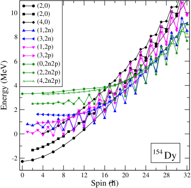
Figure 7: (Color online) Band diagram for ¹⁵⁴Dy nucleus. The labels (0,0), (2,0), (4,0), (1,2n), (3,2n), (1,2p), (3,2p), (0,2n2p) (2,2n2p) and (4,2n2p) correspond to ground, $\gamma$, 2$\gamma$, two neutron-aligned, $\gamma$-band based this two neutron-aligned state, two proton-aligned, $\gamma$-band built on this two proton-aligned state, two-neutron plus two-proton aligned, $\gamma-$ and $\gamma\gamma-$ band built on this four-quasiparticle state.

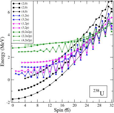
Figure 8: (Color online) Band diagram for ²³⁸U nucleus. The labels (0,0), (2,0), (4,0), (1,2n), (3,2n), (1,2p), (3,2p), (0,2n2p) (2,2n2p) and (4,2n2p) correspond to ground, $\gamma$, 2$\gamma$, two neutron-aligned, $\gamma$-band on this two neutron-aligned state, two proton-aligned, $\gamma$-band on two this proton-aligned state, two-neutron plus two-proton aligned, $\gamma-$ and $\gamma\gamma-$ band built on this four-quasiparticle state.

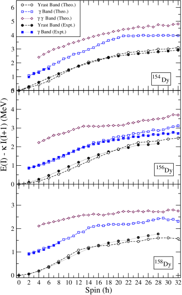
Figure 9: (Color online) Comparison of the measured energy levels of yrast-, $\gamma$-, and $\gamma$$\gamma$-bands for ^154,156,158Dy nuclei and the results of TPSM calculations. The scaling factor $\kappa$ appearing in the y-axis is defined as $\kappa=32.32A^{-5/3}$. Data is taken from Refs. [84, 85, 86].

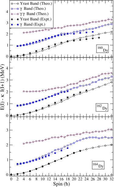
Figure 10: (Color online) Comparison of the measured energy levels of yrast-, $\gamma$-, and $\gamma$$\gamma$-bands for ^160,162,164Dy nuclei and the results of TPSM calculations. The scaling factor $\kappa$ appearing in the y-axis is defined as $\kappa=32.32A^{-5/3}$. Data is taken from Refs. [87, 88, 89, 90].

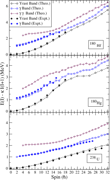
Figure 11: (Color online) Comparison of the measured energy levels of yrast-, $\gamma$-, and $\gamma$$\gamma$-bands for ¹⁸⁰Hf, ¹⁸⁰Hg and ²³⁸U nuclei and the results of TPSM calculations. The scaling factor $\kappa$ appearing in the y-axis is defined as $\kappa=32.32A^{-5/3}$. Data is taken from Refs. [91, 92, 93].

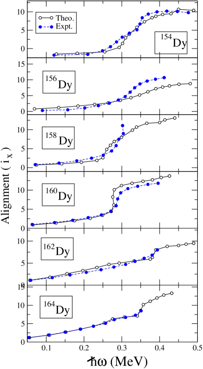
Figure 12: ( Color online) Comparison of the aligned angular momentum $i_{x}$) as a function of frequency, obtained from the measured energy levels as well as those calculated from the TPSM results, for ^154-164Dy nuclei.

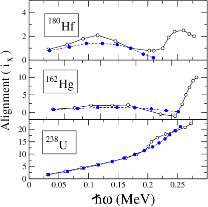
Figure 13: ( Color online) Comparison of the aligned angular momentum $i_{x}$) as a function of frequency, obtained from the measured energy levels as well as those calculated from the TPSM results, for ¹⁸⁰Hf, ¹⁸⁰Hg and ²³⁸U nuclei.

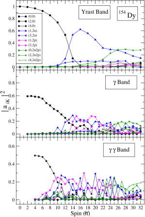
Figure 14: (Color online) Probability of various projected K-configurations in the wavefunctions of the yrast-, $\gamma-$ and $\gamma\gamma-$bands in ¹⁵⁴Dy.

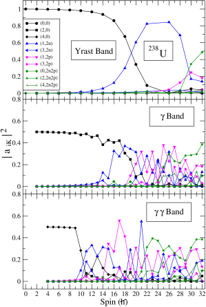
Figure 15: (Color online) Probability of various projected K-configurations in the wavefunctions of the yrast-, $\gamma-$ and $\gamma\gamma-$bands in ²³⁸U.

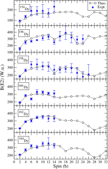
Figure 16: (Color online) Comparison of experimental and calculated $B(E2)$ for ^154-164Dy. Data is taken from Refs. [84, 94, 95, 96, 97, 98].

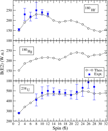
Figure 17: (Color online) Comparison of experimental and calculated $B(E2)$ for ¹⁸⁰Hf, ¹⁸⁰Hg and ²³⁸U . Data is taken from Refs. [92, 99].

It is expected that $\gamma$-bands based on the multi-quasiparticle states should be more wide spread in nuclear periodic table. In the following we shall report a recent study for ⁶⁸Ge where multiple s-bands are also observed and it is shown that one of the observed s-band in ⁶⁸Ge has the structure of the $\gamma$-band built on the two-quasineutron configuration. TPSM calculations for ⁶⁸Ge have been performed with the deformation parameters, $\epsilon=0.22$ and $\epsilon^{\prime}=0.16$ using the oscillator space of $N=3,4$ and $5$ (both for protons and neutrons) and the pairing strengths of $G_{1}=20.82$ and $G_{2}=13.58$. Fig. 3 is the obtained band diagram for ⁶⁸Ge and it is seen that $\gamma$-band depicts quite large odd-even staggering with the even-spin members closely following the ground-state band. It is further noted that ground-state band is crossed by two-quasiparticle band having $(1,2n)$ and $(3,2n)$ configurations at I = 8. These two bands are two-neutron aligned and the $\gamma$-bands built on this two-neutron state. The odd-spin members from the two-neutron $\gamma$-band form the yrast states from I = 9 to 13. It is also evident from Fig. 3 that two-aligned band having $(1,2p)$ configuration also crosses the ground-state band at I = 10 and from I = 14 the four-quasiparticle formed from two-neutron plus two-proton configuration become lowest in energy.

The band structures obtained after diagonalization are displayed in Fig. 4 along with the experimental data which depicts multiple s-bands above the ground-state band. It is evident from the figure that TPSM approach reproduces the observed band structures remarkably well. TPSM also predicts many new states for the $\gamma$-band and also a few lower states for the bands labelled as $(1,2p)$ and odd-spin member of $(3,2n)$. These levels have been assigned based on the dominant components in the calculated wavefunctions plotted in Fig. 5. The ground-state band, shown in the top panel of Fig. 5, has the dominant component, as expected, of $(0,0)$ for I = 0, 2 and 4. For I = 6, the contribution of the two-neutron aligned state having $(1,2n)$ configuration becomes equally important. It is noted from the wavefunction analysis that two observed s-bands beginning with I = 8 have dominant components of $(1,2n)$ and $(3,2n)$ configurations and, therefore, both these bands have neutron configuration and one of them is the $\gamma$-band based on the two-quasineutron configuration. The third observed s-band beginning with I = 12 has the $(1,2p)$ configuration. It needs to be clarified that it is somewhat erraneous to label these bands with a specific two-quasiparticle configuration as there is a substantial mixing and further for high-spin states four-quasiparticle states become lower in energy.

It is quite clear from above discussion that the lowest two observed s-bands have both neutron structure and the third s-band has the proton structure. The g-factor measurements have been performed for the lowest two s-bands and both are confirmed to have neutron configuration and, therefore, validating the TPSM predictions [82] as the second s-band is the $\gamma$-band built on first s-band and both originate from their same intrinsic configuration.

We have also evaluated the intra-band BE2 transition probabilities for various band structures discussed above and are plotted in Fig. 6. Measured BE2 values are also available for some transitions have been depicted in the figure. For the g-band, the experimental values are well reproduced by the TPSM calculations, however, disagreement is clearly seen for the I=10 transition in the two- quasineutron band. More experimental data is needed to test the predictions of the TPSM in detail.

3.2 Systematic investigation of $\gamma$-band structures in Dy, Hf, Hg and U nuclei

A systematic investigation of the band structures observed in ^154-164Dy, ¹⁸⁰Hf, ¹⁸⁰Hg and ²³⁸U nuclei have been performed. These nuclei have been chosen in the present study as $\gamma$-bands are known up to highest spin and it is possible to test the predictions of the TPSM approach in the limit of largest angular momemtum. TPSM calculations for these nuclei have been performed with the deformations listed in Table 2 in the shell model space with N $=$ 4, 5, 6 for neutrons and N $=$ 3, 4, 5 for protons and the pairing strength parameters of $G_{1}=21.24$ and $G_{2}=13.86$. As representative exmples, the band diagrams for ¹⁵⁴Dy and ²³⁸U are displayed in Figs. 7 and 8. In the band diagram, the ground-state band having $(0,0)$ configuration is crossed at I=14 by two-neutron aligned state configuration, $(1,2n)$. Further, it is noted that four-quasiparticle configuration, $(2,2n2p)$, crosses the two-neutron state at I=26 and above this spin value, it is expected that four-quasiparticle configurations will dominate the yrast band.

The band diagram for ²³⁸U is displayed in Fig. 8. The TPSM calculations for this system were carried out within the space of N $=$ 5, 6, 7 for neutrons and N $=$ 4, 5, 6 for protons and with the pairing strengths of $G_{1}=16.80$ and $G_{2}=12.80$. It is noted from the figure that the first crossing due to alignment of two-neutrons occurs at I = 20 and the second due to the alignment of two-neutrons plus two-protons occurs at I=30. The two-proton aligned band is seen to remain always higher in energy as compared to the neutron-aligned configuration.

The projected energies for yrast-, $\gamma$- and $\gamma\gamma$- bands, obtained after diagonalization of the shell model Hamiltonian, are plotted in Figs.  9, 10 and 11 along with the available experimental data. To have a better comparison between theoretical and experimental energies, these quantities have been subtracted by a core contribution. It is evident from the three figures that observed yrast bands in all the studied nuclei are reproduced fairly well by the TPSM calculations. For the $\gamma$-bands, the agreement between observed and calculated energies is also quite good, except that some deviations are noted in ¹⁵⁶Dy and ¹⁶⁰Dy for high-spin states above I = 22. These deviations are also noted in some of the yrast bands and are expected since for spin above $22\hbar$ the contributions from negleced four-quasineutron and four-quasiproton configurations are anticipated to become important.

$\gamma\gamma$-bands have not been observed in any of the studied nuclei and it is noted from Figs.  9, 10 and 11 that predicted band heads of these bands are quite high in energy (more than 2 MeV), but it is noted that for high-spin states these bands become quite close to the $\gamma$-bands and it should be possible to populate them at higher spin.

To probe the crossing features in the studied nuclei, the alignments of the ^154-164Dy,¹⁸⁰Hf, ¹⁶²Hg and ²³⁸U nuclei are displayed in Figs.  12 and 13 as a function of the rotational frequency. In the experimental alignment plot of ¹⁵²Dy, two upbends are clearly observed whereas in the theoretical plot only a broad upbend is noted. These upbends are due to the crossing of the aligned quasiparticle configurations along the yrast line. In order to investigate the structural changes as a function of angular momentum, the wavefunctions are plotted in Fig.  14. In the top panel of this figure, the yrast wavefunction depicts the first crossing at I = 14 as due to the alignment of two-quasineutrons, $(1,2n)$, and the second crossing at I=18 arises from the alignment of four-quasiparticle configuration, $(2,2n2p)$. The broad upbend noted in the alignment figure is due to combination of these crossings. In the experimental plot, the two crossings are clearly evident and this indicates that interaction among the crossing bands is overpredicted by the TPSM calculations. Fig.  14 also depicts the wavefunctions for the $\gamma$- and $\gamma\gamma$-bands and $\gamma$-band up to I = 12 has the expected dominat component of $(2,0)$. However, above this spin value, $\gamma$-band is a mixture of many different configurations and ceases to be called as the $\gamma$-band. $\gamma\gamma$-band has the expected structure of $(4,0)$ configuration up to I = 9 and above this spin value it ceases to be called as $\gamma\gamma$-band as well.

TPSM calculated alignment for ¹⁵⁶Dy, shown in the second panel of Fig. 12, again shows smoother behaviour as compared to the experimental alignment and is an indication that interaction among the bands is overestimated in the calculated alignment. For ^154-164Dy, shown in Fig. 12, and for ¹⁸⁰Hf, ¹⁶²Hg and ²³⁸U, depicted in Fig. 13, the agreement between the calculated and the experimental values is better than the previous two cases.

The wavefunctions for the yrast-, $\gamma-$ and $\gamma\gamma$-bands are displayed in Fig. 15 for ²³⁸U. The cross over between the ground-state configuration and the two-neutron aligned band is noted at I = 20 for the yrast band. Above I=26, two-proton aligned configuration is also noted to become important and above I=30, the four-quasipartcle configuration becomes dominant. For the $\gamma$-band, $(0,2)$ is the dominant configuration up to I=16, but above this spin value it is a highly mixed band. For $\gamma\gamma$-band, $(0,4)$, is the dominant configuration up to I=10 and above this spin, it is again a highly mixed band.

The measured BE2 transition probabilities are available along the yrast band for most of the nuclei studied in this section and are depicted in Figs. 16 and 17 along with the calculated BE2 transitions using the TPSM wavefunctions and the projected expression given in Eq. 19. It is evident from the figure that calculated BE2 reproduce the known transitions remarkably well, in particular, the drops in the measured transitions for ¹⁵⁶Dy, ¹⁵⁸Dy and ²³⁸U. The first drop in the transitions are related to the crossing of two-quasineutron aligned band with the ground-state band and the second drop is due to the crossing of four-quasiparticle composed of two-quasineutron and two-quasiproton aligned configuration. TPSM results also depict two drops for ¹⁵⁶Dy, although, not very pronounced and are due to two crossings evident from the wavefunction analysis. These crossings are not apparent in the alignment plot of Fig. 12, but are noted in the BE2 transitions as these are more senstive to the structural changes as compared to the quantities derived from the energies.

3.3 Chiral symmetry and doublet band structures

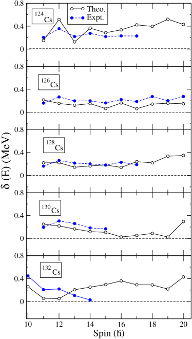
Figure 18: (Color online) Energy difference, $\delta(E)$, between doublet bands for a given spin. Data has been taken from Refs. [100, 101, 102, 103, 104, 105].

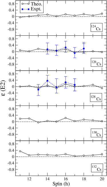
Figure 19: (Color online) Comparison of the TPSM and experimental values of $\epsilon$(E2) as a function of spin. Data has been taken from Refs. [100, 101, 102, 103, 104, 105].

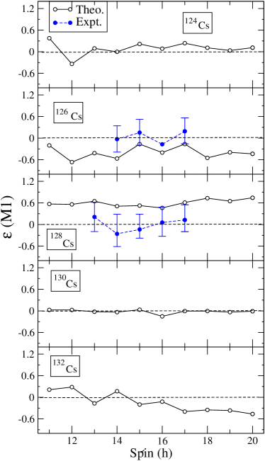
Figure 20: (Color online) Comparison of the TPSM and experimental values of $\epsilon$(M1) as a function of spin. Data has been taken from Refs. [100, 101, 102, 103, 104, 105].

The spontaneous symmetry breaking mechanism has played a central role in elucidating the intrinsic structures of quantum many body system [106]. What all is possible from the experimental analysis of a bound quntum many-body system is a set of energy levels that are labelled by the quantum numbers related to the symmetries preserved by the system. For instance, for the case of atomic nucleus the energy levels are labelled by angular-momentum and parity quantum numbers that are related to the rotational and reflection symmetries. It is through breaking of these symmetries that provides an insight into the excitation modes of the atomic nucleus. The most celebrated model that employs the symmetry breaking mechanism is the Nilsson model. This model breaks the rotational symmetry and has provided invaluable information on the structures of deformed nuclei [107]. The observation of the rotational band structures built on each intrinsic state is a manifestation of the breaking of this symmetry [108, 109].

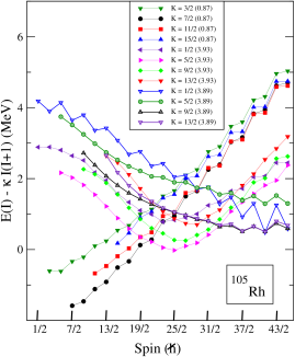
Figure 21: (Color online) The angular-momentum projected bands obtained for different intrinsic K-configuration, given in legend box, for ¹⁰⁵Rh isotopes. The energies of the quasiparticle states are given in the parenthesis. The scaling factor $\kappa$ appearing in the y-axis is defined as $\kappa=32.32A^{-5/3}$.

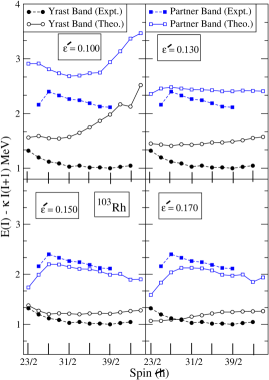
Figure 22: (Color online) Comparison of the measured energy levels of of ¹⁰³Rh nucleus and the results of TPSM calculations. The scaling factor $\kappa$ appearing in the y-axis is defined as $\kappa=32.32A^{-5/3}$.

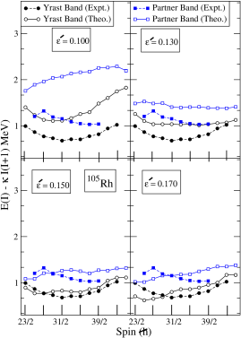
Figure 23: (Color online) Comparison of the measured energy levels of of ¹⁰⁵Rh nucleus and the results of TPSM calculations. The scaling factor $\kappa$ appearing in the y-axis is defined as $\kappa=32.32A^{-5/3}$.

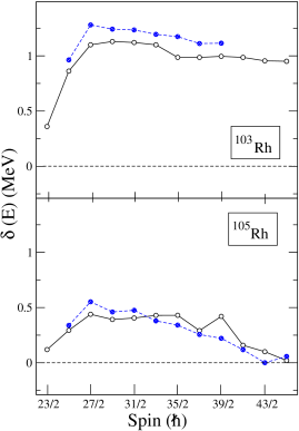
Figure 24: (Color online) Energy difference, $\delta(E)$, between the doublet bands and plotted as a function of spin for the two studied Rh-isotopes.

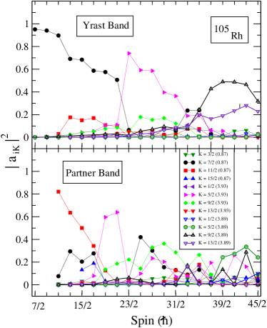
Figure 25: (Color online) Probability of various projected K-configurations in the wavefunctions of the yrast and the first excited bands for ¹⁰⁵Rh.

In recent years, it has been also demonstrated that doublet band structures observed in some odd-odd and odd-mass nuclei may be a manifestation of the breaking of the chiral symetry in the intrinsic frame of reference [110, 111, 112, 113, 114]. The chiral symmetry is possible for nuclei having triaxial shapes with total angular momentum having components along all the three mutually perpendicular axis. In odd-odd nuclei, the three angular-momentum vectors that form the chiral geometry are that of core and of valence neutron and proton. The three angular-momentum vectors can either form left- or right-handed system and can be transformed into each other with the chiral symmetry transformation operator, $\hat{T}~{}\hat{R}_{y}$, where $\hat{T}$ is the time-reversal operator and $\hat{R}_{y}$ is the rotation by $180^{0}$ about y-axis [115]. The chiral dynamical variable so called “handedness” ($\sigma$) is not a measurable quantity and what is measurable in the laboratory frame is the set of states of chiral doublet bands which have a well defined value of complementary variable, the chirality ($\Sigma$). In the strong chiral symmetry breaking limit with the three angular-momentun vectors perpendicular to each other, $\sigma$ assumes the values of $\pm 1$. The left- and right-handed states are well separated and there is no possibility of tunneling between the two states. This results into two degenerate doublet bands in the laboratory frame of reference.

For the weak chiral symmetry breaking, the three angular-momentum vectors are not orthogonal, which as a matter of fact is true in most of the physical situations, and the handedness variable takes the value between +1 and -1 [the value of 0 corresponds to the planar situation]. For this case, the tunneling between the two states takes place and in the laboratory frame this corresponds to the mixing of the two solutions with the result that two bands tend to be non-degenerate.

It is evident from the above discussion that a fingerprint of the chiral symmetry is the energy difference between the states of the doublet bands. In Fig. 18, this energy difference, $\delta(E)$, is plotted for odd-odd Cs-isotopes [24] using both observed and TPSM calculated energies. The doublet band observed in these nuclei have been proposed to arise from the breaking of the chiral symmetry mechanism. It is apparent from the figure that $\delta(E)$ varies from 0.2 to 0.4 for most of the cases. As already pointed out above, for the case of strong chiral symmetry breaking this value should be close to zero and also it should be constant as a function of angular-momentum [116]. It is noted from Fig. 18 that $\delta(E)$ varies with angular-momentum, in particular, for heavier Cs-isotopes and, therefore, it is difficult to make a definitive statement on the chiral nature of the observed doublet bands for heavier Cs-isotopes.

Further, it has been demonstrated in Ref. [116] that similar analysis as that for the energies can be also performed for the transition probabilities as chiral symmetry operator commutes, not only with the Hamiltonian, but also with the electromagnetic transition operators. The deviation between the yrast and the partner bands for the transition probabilities B$(\lambda\mu;I_{i}\rightarrow I)$ is defined as [116]

$$\epsilon(\lambda\mu;I_{i})=\frac{A-B}{A+B},$$

where

$$A=\sqrt{(2I_{i}+1)B_{yrast}(\lambda\mu;I_{i}\rightarrow I)},$$

$$B=\sqrt{(2I_{i}+1)B_{side}(\lambda\mu;I_{i}\rightarrow I)}.$$

The above quantity is displayed in Figs. 19 and 20 for the $E2$ and $M1$ transitions using the TPSM expressions and wavefunctions. The figures also display the experimental values, wherever available. It is evident from Fig. 19 that calculated values for $E2$ transitions are close to zero line for most of the cases and the experimental values available for ¹²⁶Cs and ¹²⁸Cs are well reproduced by the TPSM approach. The deviations for the $M1$ transitions, depicted in Fig. 20, are again noted to be close to zero line for the light Cs-isotopes. For the heavier Cs-isotopes, in particular, for ¹²⁸Cs, $\epsilon(M1)$ is somewhat larger and varies with spin.

For odd-mass nuclei, the three angular-momentum vectors that form chiral geometry are that of core, odd-proton (neutron) and a pair of neutrons (protons). It has been proposed that in odd-proton ¹⁰³Rh and ¹⁰⁵Rh isotopes that first excited band is the normal $\gamma$-band up to spin, I=21/2, but above this spin value this band forms the chiral partner of the yrast band. In order to investigate how $\gamma$-bands in these isotopes are transformed into the conjectured chiral bands, we have carried out TPSM study for these isotopes [23] within the space N $=$ (3, 4, 5) for neutrons and (2, 3, 4) for protons, and pairing strengths of $G_{1}=20.25$ and $G_{2}=16.20$.

As an illustrative example, the band diagram for ¹⁰⁵Rh is shown in Fig. 21 and in order to have a better visualization of the bands, the energies have been subtracted by a core contribution. The ground-state band has the intrinsic configuration of one quasiparticle with K=7/2. For odd-mass nuclei, the $\gamma$-band head has two possible configurations with $K_{g}=K\pm 2$, resulting into $K_{g}=11/2$ and $3/2$. Both these $\gamma$-bands are shown in Fig. 21 with $K_{g}=11/2$ being favoured in energy. It is noted from the figure that the ground-state band is crossed at I=19/2 by another band having K=5/2 which is a three-quasiparticle state. It is also seen that the $\gamma$-band built on this three-quasiparticle state having K=9/2 also crosses the ground-state configuration at I=23/2. There is a further simultaneous crossing by two three-quasiparticle bands having K=9/2 and 13/2 with intrinsic energy of 3.89 MeV at I=33/2.

The projected bands depicted in Fig. 21 and many more [around forty for each angular-momentum] are employed to diagonalize the shell model Hamiltonian as explained earlier. The bands obtained after band mixing are shown in Figs. 22 and 23 for ¹⁰³Rh and ¹⁰⁵Rh, respectively. The results of yrast and the first excited band are only shown above I=23/2$~{}\hbar$ as they have been proposed to originate from the chiral symmetry breaking above this spin value. It is evident from the two figures that only for the optimum triaxial deformation of $\epsilon^{\prime}=0.15$ [$\gamma=28^{0}$ for¹⁰³Rh and $\gamma=33^{0}$ for¹⁰⁵Rh], a good agreement is obtained between theoretical and the experimetal energies. In Fig. 24, $\delta(E)$ is displayed as a function of angular momentum for the isotopes and it is quite evident that deviation is quite large and, therefore, it is difficult to classify these doublet bands as chiral partners.

In order to probe further the evolution of the yrast and the first excited band structures with spin, the wavefunctions of the two bands are plotted in Fig. 25 for ¹⁰⁵Rh as a representative case. It is noted from the upper panel that yrast band up to I=21/2$~{}\hbar$ has the dominant K=7/2 configuration and above this spin value it is K=5/2 three-quasiparticle configuration that is important. It is also seen that above I=21/2$~{}\hbar$, the three quasiparticle configuration with K=9/2 dominate the yrast states. The first excited band from I=11/2$~{}\hbar$ up to I=17/2$~{}\hbar$ has the expected dominant component of K=11/2 which is the $\gamma$-band built on the ground-state configuration. However, above I=17/2$~{}\hbar$, it is a highly mixed state and ceases to be a $\gamma$-band.

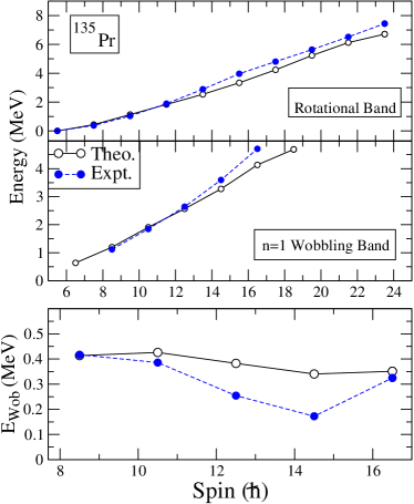
Figure 26: (Color online) Top two panels depict comparison between the experimental and TPSM results for the yrast and n=1 wobbling bands in ¹³⁵Pr. Bottom panel shows the comparison of the variation of wobbling frequency with spin.

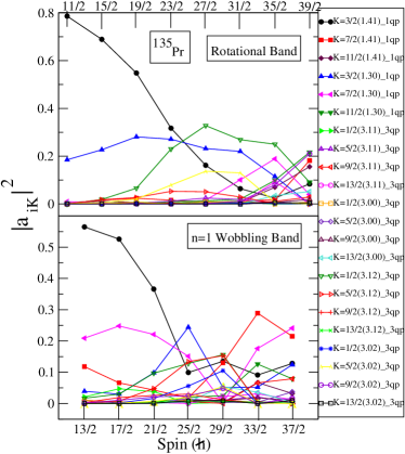
Figure 27: (Color online) Probability of various projected K-configurations in the wavefunctions of the yrast and the wobbling n=1 bands in ¹³⁵Pr. The contributions from various configurations are labelled by $K$, intrinsic energy and the rank.

3.4 Wobbling Motion

Wobbling motion like chiral symmetry, discussed above, is possible only for triaxial nuclei. This mode was predicted by Bohr and Mottelson in late sixties [6] for even-even nuclei and it was shown that the frequency of the wobbling mode is proportional to angular momentum, I with enhanced $\Delta~{}I=1$, E2 inter-connecting transitions. It has been recently shown that for odd-mass nuclei, the wobbling mode is modified depending on the direction of the angular-momentum vector of the odd-particle. For systems with angular-momentum of the odd-particle aligned along the medium axis of the core which has largest moment of inertia (referred to as longitudinal mode) the wobbling frequency decreases with spin. This frequency increases if angular-momentum of the last particle is anti-parallel to the medium axis and has been called as the transverse mode. The wobbling frequency is given by [117]

$$\begin{split}E_{wob}(I)&=E(I,n_{\omega}=1)\\ &-\frac{[E(I-1,n_{\omega}=0)+E(I+1,n_{\omega}=0)]}{2}.\end{split}$$

In the present work we have performed TPSM analysis to describe the observed band structures and the transverse wobbling mode in ¹³⁵Pr nucleus. These calculations have been performed with the deformation parameters, $\epsilon=0.16$ and $\epsilon^{\prime}=0.11$ within the configuration space of N$=3,4,5$ major shells for neutrons and N$=2,3,4$ for protons; and with the pairing interaction parameters, $G_{1}=20.12$ and $G_{2}=13.13$. The results obtained after diagonalization of the shell model Hamiltonain are presented in Fig. 26. In the top two panels of the figure, the results are compared for the yrast and the n=1 wobbling bands. In the bottom panel, the calculated wobbling frequency calculated from the TPSM energies is compared with the frequency obtained from the measured energies. It is evident from the figure that wobbling frequency from TPSM depicts less drop with spin as compared to the frequency obtained from the measured energies.

The wavefunctions for the yrast and the n=1 wobbling bands are depicted in Fig. 27 and it is evident that three-quasiparticle band crosses the one-quasipartice at I=25/2$~{}\hbar$ for both the bands. It turns out that this crossing occurs much earlier in ¹³³La and plays a vital role in understanding the longitudinal wobbling mode observed recently for this system [118]. The calculations reported here are preliminary and we are in the process of performing a detailed analysis of the wobbling motion for all the nuclei where it has been observed.

4 Summary and Future Prospects

During the last decade, research in nuclear theory has witnessed a discernable progress in the development of state-of-the-art models and techniques to elucidate the rich variety of shapes and structures in nuclei. There is a great optimism that in the coming years it should be possible to apply these Ab-initio methods to investigate majority of the properties all across the nuclear periodic table with the availability of more powerful computing facilities. However, at the moment these methods have limited applicability and are used to describe nuclei in lighter mass regions only. To study, for instance, the rich band structures observed in medium and heavy mass regions, alternative methods with moderate computational requirements ought to be explored.

Recently, TPSM approach has been developed to describe the rich band structures observed in well deformed and transitional nuclei. This model employs the basis that are solutions of the triaxial Nilsson potential and then three dimensional projection is performed to project out the states with well defined angular momentum quantum number. The advantage of this approach is that systematic studies of a large class of nuclei can be performed with a minimal computational effort. As a matter of fact, already a number of systematic investigations have been undertaken using this model and it has been demonstrated to reproduce the known experimental data remarkably well. This model has been applied to investigate a broad range of properties related to the triaxial degree of freedom of the nuclear deformation.

It is known that most of the deformed nuclei are axially symmetric with well defined angular momentum projection along the symmetry axis so called the $"K"$ quantum number. Band structures in well deformed nuclei are labelled with this quantum number and transitions in these nuclei are known to follow the selection rules based on this quantum number. However, there are also many regions so called transitional regions where the axial symmetry is known to be broken and a triaxial degree of freedom plays an important role.

In most of these triaxial nuclei, $\gamma$-bands are observed which traditionally have been considered as vibrations in the non-axial degree of freedom. In the TPSM interpretation, $\gamma$-bands emerge from the projection of the K = 2 component of the triaxial vacuum configuration. $\gamma$-bands are known in some Dy, Hf, Hg and U nuclei up to very high angular momentum and in the present work we have performed a systematic investigation of these nuclei using the TPSM approach. The observed yrast and $\gamma$-bands in all these studied nuclei have been demonstrated to be well described by the TPSM calculations. Deviations have also been noted above I = 22 and a possible reason for this discrepancy could be due to neglect of the four-quasineutron and proton configurations in the present work.

The possibility of observing $\gamma$-bands based on the quasiparticle configurations has also been explored in the present work. It is quite evident from the very construction of the basis states in TPSM approach that $\gamma$-bands are possible based on each intrinsic state. $\gamma$-band based on the ground-state are quite well established and have been studied using many different approaches and methods. However, $\gamma$-bands built on the excited quasipartice configurations have remained rather abstruse as most of the earlier models didn’t consider the quasiparticle excitations. It has been demonstrated that some of the excited band structures in Ce- and Nd- isotopes are, as a matter of fact, the $\gamma$-bands based on two-quasiparticle states. In some of these isotopes, two s-bands are observed with similar g-factors and this has remained an unsolved problem for several years. In the conventional approach, two s-bands are expected to be based on neutron and proton aligned structures and, therefore, g-factors of the two s-bands should have opposite signs. Measurements of g-factors of two s-bands provide same signs for both the s-bands and, thereby, indicating that both the s-band have either proton or neutron structures. What has been shown in the TPSM studies that second s-band in many of these nuclei is the $\gamma$-band based on the two- quasineutron or proton states. As the parent band and the $\gamma$-band based on it originate from the same intrinsic configurations, two s-bands in the TPSM approach are expected to have similar g-factors. TPSM has also povided an explanation on the observation of three s-bands in ⁶⁸Ge. It has been shown that one of the s-band is the $\gamma$-band based on the two-neutron quasiparticle state.

Further, recently new observations have been made in a set of nuclei that are considered as fingerprints of the triaxial deformation. These new observations include the occurrence of doublet bands and excited bands with dominant $\Delta~{}I=1$ E2 transitions and have been regarded as manifestaions of chiral and wobbling motion in rotational nuclei. These observations are entirely as a consequence of the triaxial shape of system and are not possible in the axial limit. In the present work, the appearance of the doublet bands have been investigated for odd-odd Cs-isotopes from A = 124 to 132 and also for the odd-proton ¹⁰³Rh and ¹⁰⁵Rh isotopes. It is expected that the doublet band should be degenerate in the limit of strong chiral symmetry breaking. It has been shown that the energy difference of the Cs-isotopes for lighter isotopes is small and, therefore, may be regarded as originating from the chiral symmetry breaking mechanism. However, for heavier isotopes, the energy difference is large and also they have a considerable variation with spin and, therefore, the doublet bands cannot be considered as chiral partners. We have also evaluated the differences in the BE2 and M1 transitions and similar conclusions have been drawn from these quantities as from the energy considerations.

The high-spin doublet band structures in ¹⁰³Rh and ¹⁰⁵Rh have also been proposed to originate from chiral symmetry breaking. In the low-spin regime, these nuclei have regular $\gamma$-bands and in the high-spin region, the observed energy difference between the $\gamma$-band and the yrast sequence decrease with spin and based on this inference, the high spin band structures have been regarded as chiral partners. [For the normal $\gamma$-band, this difference remains almost constant]. It has been shown that energy difference, both experimental and theoretical, is too large as compared to the Cs-isotopes and for some angular momentum value it is more than $1~{}$MeV. It has been also demonstrated in our earlier study [35] that quadrupole moment varies with spin quite appreciably and, therefore, the doublet bands in ¹⁰³Rh and ¹⁰⁵Rh cannot be regarded as candidates for chiral symmetry breaking.

We would like to add that one of the the major problem in the TPSM model is that first of all the pairing plus quadrupole interaction used is quite rudimentary and needs to be generalised for a better desciption of the nuclear properties. Secondly, the coupling constants of the interaction are adjusted through self-consistency condition with the input deformation parameters. This means that optimum deformation value for a system under investigation should be known prior to performing the TPSM calculations. Although, the final results should be independent of the input deformation in case a very large basis set is employed in the study, however, in practice a limited basis space is employed and the results become basis dependent. In order to circumvent this problem, we are considering to fix the coupling constant of the interaction through a mapping procedure as has been done in other approaches [119, 120]. The energy surface, for instance, obtained from the density functional theory can be mapped to the surface obtained using the model interaction used in the TPSM approach with adjustable coupling constants.

There are several other possible ways of improving the predictive power of the TPSM calculations. For instance, the diagonalization of the shell model Hamiltonian is performed for a fixed value of the deformation parameter and for a more accuate description, a set of deformation values should be considered by employing the generator coordinate method (GCM). This will allow the possibility to have coupling between the $\gamma$-deformation and $\gamma-$vibrational degrees of freedom. One of the major discrepancy that has surfaced in the application of the TPSM approach is the band head energy of the $\gamma\gamma$-band [14, 15, 16]. It has been observed that for most of known cases, TPSM calculations underpredicts band head energy of this band by more than 1 MeV. It is expected that $\gamma\gamma$-band to have siginificant vibrational component because of mixing with the quasiparticle states which are close in energy. We hope that by performing GCM with both $\beta$ and $\gamma$ as generator coordinates, the $\gamma\gamma$-band and other properties shall be described more accurately. It is also quite important to include higher multi-quasiparticle states in the basis space. It has been noted in the present investigation that TPSM results tend to disagree above I = 22 and the reason for this discrepancy is the neglect of the four-proton and -neutron quasiparticle states. We are presently working to improve the TPSM approach along the lines discussed above and the results shall be presented in future publications.

Appendix

The matrix elements of the Hamiltonian and transition operators in TPSM approach are evaluated using the Wick theorem. For instance, for a two-body operator of the form $\hat{O}^{\dagger}\hat{O}$, we have

$$\hat{O}^{\dagger}\hat{O} ={\langle\hat{O}\rangle}^{2}+\langle\hat{O}\rangle\{:\hat{O}^{\dagger}:+:\hat{O}:\}+:\hat{O}^{\dagger}\hat{O}:$$

$$\equiv\hat{H}^{(0)}+\hat{H}^{(1)}+\hat{H}^{(2)}$$

where $\langle\hat{O}\rangle$ is the contraction and $:\hat{O}:$ is the normal ordered form of the operator. The rotated matrix elements of one-body and two-body operators are given by

$$\langle\hat{H}^{(1)}[\Omega]\rangle=\langle\hat{O}\rangle\{\langle:\hat{O}^{\dagger}:[\Omega]\rangle+\langle:\hat{O}:[\Omega]\rangle\}$$

$$\langle\hat{H}^{(2)}[\Omega]\rangle=\langle:\hat{O}^{\dagger}:[\Omega]\rangle\langle:\hat{O}:[\Omega]\rangle$$

where $[\Omega]=\hat{R}(\Omega)/\,<\!\hat{R}(\Omega)\!>\,$. The detailed expressions of the above rotated matrix elements are given in Ref. [34]. In TPSM approach, diagonalization of the shell model Hamiltonian follows from the Hill-Wheeler method. In this method, the following ansatz is used for wavefunction

$$|\psi\!>\,=\int d\Omega~{}F(\Omega)~{}\hat{R}(\Omega)~{}|\phi\!>\,$$ (20)

For the projection operator, the expansion coefficient in the above equation is written as

$$F(\Omega)=\sum_{IMK}\frac{2I+1}{8\pi^{2}}F^{I}_{MK}D^{I}_{MK}(\Omega)$$

Using the variational ansatz

$$\delta\big{[}\frac{\,<\!\psi|\hat{H}|\psi\!>\,}{\,<\!\psi|\psi\!>\,}\big{]}=0,$$

and substituting $|\psi\!>\,$ from Eq. (20), we obtain

$$\sum_{\kappa^{{}^{\prime}}K^{{}^{\prime}}}\{\mathcal{H}_{\kappa K\kappa^{{}^{\prime}}K^{{}^{\prime}}}^{I}-E\mathcal{N}_{\kappa K\kappa^{{}^{\prime}}K^{{}^{\prime}}}^{I}\}F^{I}_{\kappa^{{}^{\prime}}K^{{}^{\prime}}}=0,$$ (21)

where the Hamiltonian and norm kernels are given by

$$\mathcal{H}_{\kappa K\kappa^{{}^{\prime}}K^{{}^{\prime}}}^{I}=\langle\phi_{\kappa}|\hat{H}\hat{P}^{I}_{KK^{{}^{\prime}}}|\phi_{\kappa^{{}^{\prime}}}\rangle,$$

$$\mathcal{N}_{\kappa K\kappa^{{}^{\prime}}K^{{}^{\prime}}}^{I}=\langle\phi_{\kappa}|\hat{P}^{I}_{KK^{{}^{\prime}}}|\phi_{\kappa^{{}^{\prime}}}\rangle.$$

In the TPSM model, we work in a representation in which the norm matrix is diagonal, i.e.,

$$\sum_{\kappa^{{}^{\prime}}K^{{}^{\prime}}}\mathcal{N}_{\kappa K\kappa^{{}^{\prime}}K^{{}^{\prime}}}^{I}U^{\sigma}_{\kappa^{{}^{\prime}}K^{{}^{\prime}}}=n_{\sigma}U^{\sigma}_{\kappa K},$$

and solve Eq. (21) with the eigenstates of the above norm equation as the basis states.

References

- [1] R. F. Casten, Nuclear Structure from a Simple Perspective, Second Edition (Oxford University Press, 2000).
- [2] K. Kumar, Nuclear Models and Search for unity in Nuclear Physics (Universitetforlaget, Bergen, Norway, 1984).
- [3] M. G. Mayer and J. H. D. Jensen, Elementry Theory of Nuclear Shell Structure (John Wiley Sons, New York, 1955).
- [4] E. P. Grigorviev and V. G. Soloviev, Structure of Even Deformed Nuclei (Nauka, Moscow, 1974) [in Russian].
- [5] V. G. Soloviev, Theory of Complex Nuclei, translated by P. Vogel (Pergamon, Elmsford, NY, 1976).
- [6] A. Bohr and B. R. Mottelson, Nuclear Structure, Vol. II (Benjamin Inc., New York, 1975).
- [7] S. G. Nilsson, Dan. Mat. Fys. Medd. 29, 16 (1955).
- [8] J. Erler, N. Birge, M. Kortelainen, W. Nazarewicz, E. OLsen, A. M. Perhac, and M. Stoitsov, Nature 486, 509 (2012).
- [9] W. Kohn and L. J. Sham, Phys. Rev. 140, A1133 (1965).
- [10] P. Hohenberg and W. Kohn, Phys. Rev. 136, B864 (1964).
- [11] J. Dobaczewski, I. Hamamoto, W. Nazarewicz, and J. A. Sheikh, Phys. Rev. Lett. 72, 981 (1994).
- [12] M. Bender, P. H. Heenen, and P. G. Reinhard, Rev. Mod. Phys. 75, 121 (2003).
- [13] J. A. Sheikh and K. Hara, Phys. Rev. Lett. 82, 3968 (1999).
- [14] J. A. Sheikh, G. H. Bhat, Y. Sun, G. B. Vakil, and R. Palit, Phys. Rev. C 77, 034313 (2008).
- [15] J. A. Sheikh, G. H. Bhat, R. Palit, Z. Naik, and Y. Sun, Nucl. Phys. A 824, 58 (2009).
- [16] J. A. Sheikh, G. H. Bhat, Y. Sun, and R. Palit, Phys. Lett. B 688, 305 (2010).
- [17] J. A. Sheikh, G. H. Bhat, Y.-X. Liu, F.-Q. Chen, and Y. Sun, Phys. Rev. C 84, 054314 (2011).
- [18] E. Y. Yeoh, S. J. Zhu, J. H. Hamilton, K. Li, A. V. Ramayya, Y. X. Liu, J. K. Hwang, S. H. Liu, J. G. Wang, Y. Sun, J. A. Sheikh, G. H. Bhat, Y. X. Luo, J. O. Rasmussen, I. Y. Lee, H. B. Ding, L. Gu, Q. Xu, Z. G. Xiao, and W. C. Ma, Phys. Rev. C 83, 054317 (2011).
- [19] G. H. Bhat, J. A. Sheikh, Y. Sun, and U. Garg, Phys. Rev. C 86, 047307 (2012).
- [20] G. H. Bhat, J. A. Sheikh, and R. Palit, Phys. Lett. B 707, 250 (2012).
- [21] J. Sethi, R. Palit, S. Saha, T. Trivedi, G. H. Bhat, J. A. Sheikh, P. Datta, J.J. Carroll, S. Chattopadhyay, R. Donthi, U. Garg, S. Jadhav, H. C. Jain, S. Karamian, S. Kumar, M. S. Litz, D. Mehta, B.S. Naidu, Z. Naik, S. Sihotra, and P.M. Walker, Phys. Lett. B 725, 85 (2013).
- [22] G. H. Bhat, W. A. Dar, J. A. Sheikh, and Y. Sun, Phys. Rev. C 89, 014328 (2014).
- [23] G. H. Bhat, J. A. Sheikh W. A. Dar, S. Jehangir, R. Palit, and P. A. Ganai, Phys. Lett. B 738, 218 (2014).
- [24] G. H. Bhat, R. N. Ali, J. A. Sheikh, and R.Palit, Nucl. Phys. A 922, 150 (2014).
- [25] N. Rather, P. Datta, S. Chattopadhyay, G. H. Bhat, J. A. Sheikh, S. Roy, R. Palit, S. Pal, S. Saha, J. Sethi, S. Biswas, P. Singh, and H. C. Jain, Phys. Rev. Lett. 112, 202503 (2014).
- [26] C. L. Zhang, G. H. Bhat, W. Nazarewicz, J. A. Sheikh, and Yue Shi, Phys. Rev. C 92, 034307 (2015).
- [27] M. Kumar Raju, D. Negi, S. Muralithar, R. P. Singh, J. A. Sheikh, G. H. Bhat, R. Kumar, Indu Bala, T. Trivedi, A. Dhal, K. Rani, R. Gurjar, D. Singh, R. Palit, B. S. Naidu, S. Saha, J. Sethi, R. Donthi, and S. Jadhav Phys. Rev. C 91, 024319 (2015).
- [28] W. A. Dar, J. A. Sheikh, G. H. Bhat, R. Palit, R. N. Ali, and S. Frauendorf, Nucl. Phys. A 933, 123 (2015).
- [29] P. Ring and P. Schuck, The Nuclear Many Body Problem (Springer-Verlag, New York), (1980).
- [30] K. Hara and S. Iwasaki, Nucl. Phys. A 332 (1979) 61.
- [31] K. Hara and S. Iwasaki, Nucl. Phys. A 348 (1980) 200.
- [32] Y. Sun, K. Hara, J. A. Sheikh, J. G. Hirsch, V. Velazquez, and M. Guidry, Phys. Rev. C 61, 064323 (2000).
- [33] S. G. Nilsson, C. F. Tsang, A. Sobiczewski, Z. Szymanski, S. Wycech, C. Gustafson, I. Lamm, P. Moller, and B. Nilsson, Nucl. Phys. A 131, 1 (1969).
- [34] K. Hara and Y. Sun, Int. J. Mod. Phys. E 4, 637 (1995).
- [35] J. A. Sheikh, Y. Sun, and R. Palit, Phys. Lett. B 507,eg12 115 (2001).
- [36] Y. Sun and J. A. Sheikh, Phys. Rev. C 64, 031302 (2001).
- [37] R. Palit, J. A. Sheikh, Y. Sun, and H. C. Jain, Nucl. Phys. A 686, 141 (2001).
- [38] F.-Q. Chen, Y. Sun, P. M. Walker, G. D. Dracoulis, Y. R. Shimizu, and J. A. Sheikh, J. Phys. G 40, 015101 (2013).
- [39] Y. Sun, G.-L. Long, F. Al-Khudair, and J. A. Sheikh, Phys. Rev. C 77, 044307 (2008).
- [40] Y. Sun and J. L. Egido, Nucl. Phys. A 580, 1 (1994).
- [41] P. Möller and J.R. Nix, At. Data Nucl. Data Tables 59, 185 (1995).
- [42] P. Bonche, J. Dobaczewski, H. Flocard, and P. -H. Heemen, Nucl. Phys. A 530, 149 (1991).
- [43] M. Matsuo and K. Matsuyanagi, Prog. Theor. Physc. 74, 1227 (1985); 76, 1235 (1987).
- [44] V. G. Soloviev and N. Yu. Shirikova, Z. Phys. A 301, 263 (1981).
- [45] J. Leandri and R. Piepenbring, Phys. Rev. C 37, 2779 (1988).
- [46] M. K. Jammari and R. Piepenbring, Nucl. Phys. A 487, 77 (1988).
- [47] M. Matsuo and K. Matsuyanagi, Prog. Theor. Phys. 78, 591 (1987).
- [48] E. R. Marshalek and R. G. Nazinithdinov, Phys. Lett. B 300, 199 (1992).
- [49] H. G. Borner and J. Joli, J. Phys. G 19, 217 (1993).
- [50] D. G. Burke and P. C. Sood, Phys. Rev. C 51, 3525 (1994).
- [51] A. Arima and F. Iachello, Phys. Rev. Lett. 35, 1069 (1975).
- [52] N. Yoshinaga, Y. Akiyama, and A. Arima, Phys. Rev. 56, 1116 (1986).
- [53] O. Castanos, J. P. Draayer, and Y. Leschber, Ann. Phys. (New York) 180, 290 (1987).
- [54] P. E. Garrett, M. Kadi, Min Li, C. A. McGrath, V. Sorokin, M. Yehand, and S. W. Yates, Phys. Rev. Lett. 78, 4545 (1997).
- [55] E. R. Marshalek and J. Weneser, Phys. Rev. C 2, 1682 (1970).
- [56] J. L. Egido, H. J. Mang, and P. Ring, Nucl. Phys. A 339, 390 (1980).
- [57] A. S. Davydov and G. F. Filippov, Nucl. Phys. 8, 237 (1958).
- [58] A. Guessous, N. Schulz, W. R. Phillips, I. Ahmad, M. Bentaleb, J. L. Durell, M. A. Jones, M. Leddy, E. Lubkiewicz, L. R. Morss, R. Piepenbring, G. Smith, W. Urban, and B. J. Varley, Phys. Rev. Lett. 75, 2280 (1995).
- [59] X. Wu, A. Aprahamian, S. M. Fischer, W. Reviol, G. Liu, and J. X. Saladin, Phys. Rev. C 49, 1837 (1994).
- [60] X. Wu, A. Aprahamian, S. M. Fischer, W. Reviol, G. Liu, and J. X. Saladin, Phys. Lett. B 316, 235 (1993).
- [61] H. G. Borner, J. Jolie, S. J. Rabinson, B. Krusche, R. Piepenring, R. F. Casten, A. Aprahamian, and J. P. Draayer, Phys. Rev. Lett. 66, 691 (1991).
- [62] M. K. Jammari and R. Piepenbring, Nucl. Phys. A 481, 81 (1988).
- [63] V. G. Soloviev and N. Yu. Shirikova, Z. Phys. 324, 393 (1986); Phys. G 148, S39 (1988).
- [64] A. Bohr and B. R. Mottelson, Phys. Scr. 25, 28 (1982).
- [65] D. G. Burke, Phys. Rev. Lett. 73, 1899 (1994). 4545 (1997).
- [66] N. Minkov, S. B. Drenska, P. P. Raychev, R. P. Roussev, and D. Bonatsos, Phys. Rev. C 60, 034305 (1999).
- [67] R. F. Corminboeuf, J. Jolie, H. Lehmann, K. Fohl, F. Hoyler, H. G. Borner, C. Doll, and P. E. Garrett, Phys. Rev. C 56, R1201 (1997).
- [68] A. S. Davydov and G. F. Fillippov, Nucl. Phys. 8, 237 (1958).
- [69] C. Fahlander, A. Axelsson, M. Heinebrodt, T. Hartlein, and D. Schwalm, Phys. Lett. B 388, 475 (1996).
- [70] T. S. Dumitrescu and I. Hamamoto, Nucl. Phys. A 383, 205 (1982).
- [71] A. Zemel, C. Broude, E. Dafni, A. Gelberg, M. B. Goldberg, J. Gerber, G. J. Kumbartzki, and K. -H. Speidel, Nucl. Phys. A 383, 165 (1982).
- [72] E. Grosse, F. S. Stephens, and R. M. Diamond, Phys. Rev. Lett. 31, 480 (1973).
- [73] R. Wyss, A. Granderath, R. Bengtsson, P. Von Brentano, A. Dewald, A. Gelberg, A. Gizon, J. Gizon, S. Harrisopulos, A. Jhonson, W. Lieberz, W. Nazarwicz, J. Nyberg, and K. Schiffer, Nucl. Phys. A 505 (1989) 337.
- [74] J. A. Alcántara-Núñez, J. R. B. Oliveira, E. W. Cybulska, N. H. Medina, M. N. Rao, R. V. Ribas, M. A. Rizzutto, W. A. Seale, F. Falla-Sotelo, and K. T. Wiedemann, Phys. Rev. C 71, 054315 (2005).
- [75] E. S. Paul, P. T. W. Choy, C. Andreoiu, A. J. Boston, A. O. Evans, C. Fox, S. Gros, P. J. Nolan, G. Rainovski, J. A. Sampson, H. C. Scraggs, A. Walker, D. E. Appelbe, D. T. Joss, J. Simpson, J. Gizon, A. Astier, N. Buforn, A. Prvost, N. Redon, O. Stzowski, B. M. Nyak, D. Sohler, J. Timr, L. Zolnai, D. Bazzacco, S. Lunardi, C. M. Petrache, P. Bednarczyk, D. Curien, N. Kintz, and I. Ragnarsson, Phys Rev. C 71, 054309 (2005).
- [76] A. A. Sonzogni, Nucl. Data Sheets 103, 1 (2004).
- [77] C. M. Petrache, D. Bazzacco, S. Lunardi, C. R. Alvarez, R. Venturelli, R. Burch, P. Pavan, G. Maron, D. R. Napoli, L. H. Zhu, and R. Wyss, Phys. Lett. B 387, 31 (1996).
- [78] O. Zeidan, D. J. Hartley, L. L. Reidinger, W. Reviol, W. D. Weintraub, Y. Sun, and Jing-ye Zhang, Phys. Rev. C 66, 044311 (2002).
- [79] E. Mergel, C. M. Petrache, G. Lo Bianco, H. Hubel, J. Domscheit, N. Nenoff, A. Neuver, A. Gorgen, F. Becker, E. Bouchez, M. Houry, W. Korten, A. Bracco, N. Blasi, F. Camera, S. Leoni, F. Hannachi, M. Rejmund, P. Reiter, P. G. Thirolf, A. Astier, N. Redon, and O. Stezowski, Eur. Phys. J. A 15, 417 (2002).
- [80] D. Ward, C. E. Svensson, I. Ragnarsson, C. Baktash, M. A. Bentley, J. A. Cameron, M. P. Carpenter, R. M. Clark, M. Cromaz, M. A. Deleplanque, M. Devlin, R. M. Diamond, P. Fallon, S. Flibotte, A. Galindo-Uribarri, D. S. Haslip, R. V. F. Janssens, T. Lampman, G. J. Lane, I. Y. Lee, F. Lerma, A. O. Macchiavelli, S. D. Paul, D. Radford, D. Rudolph, D. G. Sarantites, B. Schaly, D. Seweryniak, F. S. Stephens, O. Thelen, K. Vetter, J. C. Waddington, J. N. Wilson, and C.-H. Yu, Phys. Rev. C 63, 014301 (2000).
- [81] M. B. Lewis, Nucl. Data Sheets 14, 155 (1975).
- [82] M. E. Barclay et al., J. Phys. G 12, L295 (1986).
- [83] S. Raman, C. H. Malarkey, W. T. Milner, C. W. Nestor, Jr., and P. H. Stelson, Atom. Data Nucl. Data Tables 36, 1 (1987).
- [84] C. W. Reich, Nucl. Data Sheets 110, 2257 (2009).
- [85] S. N. T. Majola, D. J. Hartley, L. L. Riedinger, J. F. Sharpey-Schafer, J. M. Allmond, C. Beausang, M. P. Carpenter, C. J. Chiara, N. Cooper, D. Curien, B. J. P. Gall, P. E. Garrett, R. V. F. Janssens, F. G. Kondev, W. D. Kulp, T. Lauritsen, E. A. McCutchan, D. Miller, J. Piot, N. Redon, M. A. Riley, J. Simpson, I. Stefanescu, V. Werner, X. Wang, J. L. Wood, C.-H. Yu, and S. Zhu, Phys. Rev. C 91, 034330 (2015).
- [86] J. Simpson, P. A. Butler, P. D. Forsyth, J. F. Sharpey-Schafer, J. D. Garrett, G. B. Hagemannl, B Herskind, and L. P. Ekstromg, J. Phys. G: Nucl. Phys. 10, 383 (1984).
- [87] A. Jungclaus, B. Binder, A. Dietrich, T. Har̈tlein, H. Bauer, Ch. Gund, D. Pansegrau, and D. Schwalmet, Phys. Rev. C 66, 014312 (2002).
- [88] C. Y. Wu, D. Cline, M. W. Simon, G. A. Davis, and R. Teng, A. O. Macchiavelli, and K. Vetter, Phys. Rev. C 64, 064317 (2001).
- [89] A. Aprahamian, X. Wu, S. R. Lesher, D. D. Warnerm W. Gelletly, H. G. Börner, F. Hoyler, K. Schreckenbach, R. F. Castene, Z. R. Shi, D. Kusnezov, M. Ibrahim, A. O. Macchiavelli, M. A. Brinkman, and J. A. Becker, Nucl. Phys. A 764, 42 (2006).
- [90] N. R. Johnson, D. Cline, S. W. Yates, F. S. Stephens, L. L. Riedinger, and R. M. Ronningen, Phys. Rev. Lett. 40, 151 (1978).
- [91] E. Ngijoi-Yogo, S. K. Tandel, G. Mukherjee, I. Shestakova, P. Chowdhury, C. Y. Wu, D. Cline, A. B. Hayes, R. Teng, R. M. Clark, P. Fallon, A. O. Macchiavelli, K. Vetter, F. G. Kondev, S. Langdown, P. M. Walker, C. Wheldon, and D. M. Cullen, Phys. Rev. C 75, 034305 (2007).
- [92] S. -C. Wu and H. Niu, Nucl. Data Sheets 100, 483 (2003).
- [93] D. Ward, H. R. Andrews, G. C. Ball, A. Galindo-Uribarri, V. P. Janzen, T. Nakatsukasa, D. C. Radford, T. E. Drake, J. DeGraaf, S. Pilotte, and Y. R. Shimizu, Nucl. Phys. A 600, 88 (1996).
- [94] R. G. Helmer, Nucl. Data Sheets 65, 65 (1992).
- [95] R. G. Helmer, Nucl. Data Sheets 101, 325 (2004).
- [96] J. K. Tuli, Nucl. Data Sheets 12, 477 (1974).
- [97] C. W. Reich, Nucl. Data Sheets 108, 1807 (2007).
- [98] B. Singh, Nucl. Data Sheets 93, 243 (2001).
- [99] E. Browne and J. K. Tuli, Nucl. Data Sheets 127, 191 (2015).
- [100] E. Grodner, I. Sankowskaa, T. Morek, S. G. Rohoziński, Ch. Droste, J. Srebrny, A. A. Pasternak, M. Kisieliński, M. Kowalczyk, J. Kownacki, J. Mierzejewski, A. Król, and K. Wrzosek, Phys. Lett. B 703, 46 (2011).
- [101] A. Gizon J. Timár, J. Gizona, B. Weiss, D. Barnéoud, C. Foin, J. Genevey, F. Hannachi, C. F. Liang, A. Lopez-Martens, P. Paris, B. M. Nyakó, L. Zolnai, J. C. Merdinger, S. Brant, and V. Paar, Nucl. Phys. A 694, 63 (2001).
- [102] H. G. Ganev and S. Brant, Phys. Rev. C 82, 034328 (2010).
- [103] E. Grodner, J. Srebrny, A. A. Pasternak, I. Zalewska, T. Morek, Ch. Droste, J. Mierzejewski, M. Kowalczyk, J. Kownacki, M. Kisieliński, S. G. Rohoziński, T. Koike, K. Starosta, A. Kordyasz, P. J. Napiorkowski, M. Wolińska-Cichocka, E. Ruchowska, W. Płóciennik, and J. Perkowski, Phys. Rev. Lett. 97, 172501 (2006).
- [104] G. Rainovski, E. S. Paul, H. J. Chantler, P. J. Nolan, D. G. Jenkins, R. Wadsworth, P. Raddon, A. Simons, D. B. Fossan, T. Koike, K. Starosta, C. Vaman, E. Farnea, A. Gadea, Th. Kröll, R. Isocrate, G. de Angelis, D. Curien, and V. I. Dimitrov, Phys. Rev. C 68, 024318 (2003).
- [105] A. J. Simons, P. Joshi, D. G. Jenkins, P. M. Raddon, R. Wadsworth, D. B. Fossan, T. Koike, C. Vaman, K. Starosta, E. S. Paul, H. J. Chantler, A. O. Evans, P. Bednarczyk, and D. Curien, J. Phys. G 31, 541 (2005).
- [106] S. Frauendorf, Rev. Mod. Phys. 73, 463 (2001).
- [107] S. G. Nilsson, Dan. Mat. Fys. Medd. 29, 16 (1955).
- [108] S. Frauendorf and J. Meng, Nucl. Phys. A 617, 131 (1997).
- [109] T. Koike, K. Starosta, and I. Hamamoto, Phys. Rev. Lett. 17, 172502 (2004).
- [110] V. I. Dimitrov, S. Frauendorf, and F. Dönau, Phys. Rev. Lett. 84, 5732 (2000).
- [111] P. Olbratowski, J. Dobazewski, J. Dudek, and W. Plöciennik, Phys. Rev. Lett. 93, 052501 (2004).
- [112] S. Q. Zhang, B. Qi, S. Y. Wang, and J. Meng, Phys. Rev. C 75, 044307 (2007).
- [113] S. Mukhopadhyay et al., Phys. Rev Lett. 99, 172501 (2007).
- [114] D. Almehed, F. Dönau, and S. Frauendorf, Phys. Rev. C 83, 054308 (2011).
- [115] K. Starosta, C. J. Chiara, D. B. Fossan, T. Koike, T. T. S. Kuo, D. R. LaFosse, S. G. Rohozinski, Ch. Droste, T. Morek, and J. Srebrny, Phys. Rev. C 65, 044328 (2002).
- [116] E. Grodner, Acta Physica Polonica B 39, 531 (2008).
- [117] J.T. Matta, U. Garg, W. Li, S. Frauendorf, A. D. Ayangeakaa, D. Patel, K. W. Schlax, R. Palit, S. Saha, J. Sethi, T. Trivedi, S. S. Ghugre, R. Raut, A. K. Sinha, R. V. F. Janssens, S. Zhu, M. P. Carpenter, T. Lauritsen, D. Seweryniak, C. J. Chiara, F. G. Kondev, D. J. Hartley, C. M. Petrache, S. Mukhopadhyay, D. Vijaya Lakshmi, M. Kumar Raju, P. V. Madhusudhana Rao, S. K. Tandel, and S. Ray, F. Dönau, Phys. Rev. Lett. 114, 082501 (2015).
- [118] S. Biswas, R. Palit, U. Garg, G. H. Bhat, S. Frauendorf, W. Li, J. A. Sheikh, J. Sethi, S. Saha, P. Singh, D. Choudhury, J. T. Matta, A. D. Ayangeakaa, W. A. Dar, V. Singh, and S. Sihotra (in preparation) (2015).
- [119] R. Rodŕiguez-Guzmán, Y. Alhassid, and G. F. Bertsch, Phys. Rev. C 77, 064308 (2008).
- [120] Y. Alhassid, G. F. Bertsch, L. Fang, and B. Sabbey, Phys. Rev. C 74, 034301 (2006).