Reference-Based Almost Stochastic Dominance Rules with Application in Risk-Averse Optimization

Abstract

Stochastic dominance is a preference relation of uncertain prospect defined over a class of utility functions. While this utility class represents basic properties of risk aversion, it includes some extreme utility functions rarely characterizing a rational decision maker’s preference. In this paper we introduce reference-based almost stochastic dominance (RSD) rules which well balance the general representation of risk aversion and the individualization of the decision maker’s risk preference. The key idea is that, in the general utility class, we construct a neighborhood of the decision maker’s individual utility function, and represent a preference relation over this neighborhood. The RSD rules reveal the maximum dominance level quantifying the decision maker’s robust preference between alternative choices. We also propose RSD constrained stochastic optimization model and develop an approximation algorithm based on Bernstein polynomials. This model is illustrated on a portfolio optimization problem.

1 Introduction

Stochastic dominance is a risk averse stochastic ordering approach (Hadar and Russell (1969), Hanoch and Levy (1969), Bawa (1975), Shaked and Shanthikumar (1994), Müller and Stoyan (2002)). Consider two random variables $X,Y\in(\Omega,\mathcal{F},P;\Theta)$ with the support $\Theta:=[\underline{\theta},\ \overline{\theta}]$. $X$ stochastically dominates $Y$ in the $m^{th}$ order if $\mathbb{E}[u(X)]\geq\mathbb{E}[u(Y)]$ for any utility function $u$ satisfying $(-1)^{k-1}u^{(k)}(x)\geq 0$, $k=1,\dots,m$, for all $x\in\Theta$ (Levy (2006), Brockett and Golden (1987)). This utility class represents basic properties of risk aversion. For example, the decision maker prefers more to less if $u^{\prime}(x)\geq 0$, is risk averse if $u^{\prime\prime}(x)\leq 0$, and becomes prudent if $u^{\prime\prime\prime}(x)\geq 0$ on $\Theta$. On the one hand, the use of stochastic dominance to compare alternatives avoids assessing the decision maker’s specific utility function which characterizes her risk attitude. Fully learning individual risk attitude is restricted with cognitive difficulty and incomplete information (Karmarkar (1978), Weber (1987)). On the other hand, stochastic dominance based preference is often unnecessarily over-conservative (Leshno and Levy (2002), Lizyayev and Ruszczyński (2012), Hu et al. (2013)). We consider the following example analogous to one given by Levy (2006). Suppose that Hannah wants to invest in one of the following lottery tickets priced at $1:

• $\bar{X}_{1}$: yielding $\$0$ with the probability of $1\%$ and $2 with the probability of $99\%$,

• $\bar{Y}_{1}$: yielding $0.01 (1 penny) with certainty.

Although $\bar{X}_{1}$ is much more attractive than $\bar{Y}_{1}$, stochastic dominance does not support the preference of $\bar{X}_{1}$ over $\bar{Y}_{1}$. In this case, the support $\Theta=[0,2]$, where $\underline{\theta}=0$ means that Hannah loses all investment and $\overline{\theta}=2$ shows that Hannah gains 100% profit. Let Hannah’s utilities at $0 and $2 be 0 and 1, respectively. It can be seen that, for the utility function $\tilde{u}(x):=\sqrt[1000]{x/2}$, we have that $\mathbb{E}[\tilde{u}(\bar{X}_{1})]\leq\mathbb{E}[\tilde{u}(\bar{Y}_{1})]$. Since $\tilde{u}$ is infinitely differentiable in $\Theta$ ($\tilde{u}^{\prime}(0)=\infty$ is allowed) and has the derivatives with alternating signs regarding the degrees of the derivatives, $\tilde{u}$ belongs to the utility class of any order stochastic dominance. The risk characterization specified by $\tilde{u}$ overvalues very small gains but completely neglects the possible difference in large gains ($\tilde{u}(x)$ has a very stiff increase for a small $x$, while being flat for a large $x$). Such behavior is quite unnatural; however, stochastic dominance requires that the preference should hold for all suitable utility functions including $\tilde{u}$.

In the paper we propose a novel concept of reference-based almost stochastic dominance (RSD). This concept provides a natural way to relax stochastic dominance by combining general and individual characterizations of risk aversion. The key idea is that, in the general utility classes, we construct a neighborhood of the decision maker’s individual utility function, and specify preference rules over this neighborhood. This relaxation is motivated by the utility theory based interpretation of stochastic dominance. Differently, Leshno and Levy (2002), Lizyayev and Ruszczyński (2012), and Hu et al. (2013) relaxed the distributionally defined forms of the first and second order stochastic dominance. Working on the CVaR based interpretation of the second order stochastic dominance, Noyan and Rudolf (2013) proposed the relaxed stochastic ordering which requires the CVaR of the preferred random variable to be larger over a shrunk set of confidence levels. Armbruster and Delage (2015) and Hu and Mehrotra (2015) developed robust expected utility maximization models which also consider individualizing the set of utility functions to meet the decision maker’s risk attitude. Armbruster and Delage (2015) used the paired game method where the decision maker’s risk attitude is partially characterized by her pairwise preference of designed lotteries. Hu and Mehrotra (2015) specified boundary conditions on utility and marginal utility functions using parametric utility assessments, and construct auxiliary conditions using both standard and paired game methods.

We address optimization problems with RSD constraints. In the literature, Dentcheva and Ruszczyński (2003, 2004) first introduced stochastic dominance constrained optimization problems, which pursue expected profit while hedging risk by choosing options preferable to a random benchmark. Since the last decade, optimization models using stochastic dominance have been the subject of theoretical considerations and practical applications in areas such as business, finance, energy and transportation (e.g. Karoui and Meziou (2006), Roman et al. (2006), Dentcheva and Ruszczyński (2006), Dentcheva et al. (2007), Luedtke (2008), Lean et al. (2010), Drapkin and Schultz (2010), Hu et al. (2012), Nie et al. (2012), Sun and Xu (2014), Haskell and Jain (2015)).

In addition, our model uses the concept of functional robustness. We specify a nonparametric shape-preserving utility neighborhood. This specification is suitable for classical nonparametric standard gamble methods and paired gamble methods such as preference comparison, probability equivalence, value equivalence, and certainty equivalence (Farquhar (1984), Wakker and Deneffe (1996), and reference therein). The functionally robust optimization was first proposed by Hu et al. (2015) in a newsvendor problem for the unknown mathematical form of the price-demand function, which is different from traditional robust approaches requiring the knowledge of the functional form (e.g. Ben-Tal and Nemirovski (1998), El Ghaoui and Lebret (1997), Bertsimas et al. (2004), Scarf (1958), Shapiro and Ahmed (2004), Delage and Ye (2010), Bertsimas et al. (2010)). To specify the uncertainty set of the price-demand function, Hu et al. (2015) consider an error allowance for the least-squares fitting at discrete data points. We generalize their approach to introduce an $\mathcal{L}_{2}$-norm based perturbation tolerance around the decision maker’s reference utility function. In the context of stochastic dominance, this tolerance is interpreted as the decision maker’s desired dominance level.

This paper is organized as follows. In Section 2, we define RSD, and use the example of Hannah’s comparing lotteries to illustrate the desired dominance level. Section 3 develops an optimization model with RSD constrains, and discusses its approximation using Bernstein polynomials. We analyze the approximation error in relation to the degree of Bernstein polynomials. In Section 4, to solve the approximation problem, we develop a cut-generation algorithm. The effect of the RSD constraint and the complexity of the algorithm are illustrated in Section 5 by using the financial portfolio optimization problem given in Dentcheva and Ruszczyński (2003). Section 6 concludes.

2 Reference-Based Almost Stochastic Dominance (RSD)

In this section we discuss the concept of RSD, which is specified as a preference relation based on the neighborhood of the decision maker’s reference utility function. Without loss of generality, assume that the reference utility function, denote by $u_{ref}$, is increasing on $\Theta$ and satisfies $u_{ref}(\underline{\theta})=0$ and $u_{ref}(\overline{\theta})=1$.

Definition 2.1

For the reference utility function $u_{ref}$, a random variable $X\in(\Omega,\mathcal{F},P;\Theta)$ is preferred to another random variable $Y\in(\Omega,\mathcal{F},P;\Theta)$ in the $m^{th}$ order reference-based almost stochastic dominance (RSD) for a given $\epsilon\in[0,1]$ (written as $X\succeq^{\epsilon}_{(m)}Y$ w.r.t. $u_{ref}$), if

$$\mathbb{E}[u(X)]\geq\mathbb{E}[u(Y)],$$

for any utility function $u$ satisfying

1. for any $x\in\Theta$, $(-1)^{i-1}u^{(i)}(x)\geq 0$, $i=1,\dots,m$.

2. $u(\underline{\theta})=u_{ref}(\underline{\theta})=0$, and $u(\overline{\theta})=u_{ref}(\overline{\theta})=1$,

3. $\|u-u_{ref}\|_{\mathcal{L}_{2}}\leq\epsilon$ ($\|f\|_{\mathcal{L}_{2}}:=\left(\int_{\Theta}f(t)^{2}\mu(dt)\right)^{1/2}$ for a given nonnegative measure $\mu$ with $\mu(\Theta)=1$),

4. for any $x\in\Theta$, $u(x)\leq\frac{M}{1-\epsilon}u_{ref}(x)$, for a fixed $M>1$ (if $\epsilon=1$, then $u(x)<\infty$).

Condition (A1) represents the utility class required by the $m^{th}$ order stochastic dominance to describe the basic properties of risk aversion. Condition (A2) is the normalization of utility functions. Condition (A3) generates a neighborhood around reference utility function $u_{ref}$. The neighborhood is a closed ball, with the radius $\epsilon$, on the $\mathcal{L}_{2}$-normed space with the measure $\mu$ on $\Theta$. Note that conditions (A1) and (A2) ensure that, if $\epsilon=1$, condition (A3) becomes redundant, and RSD in this case represents stochastic dominance. To further interpret $\epsilon$, we need to define the maximum dominance level as follows.

Definition 2.2

For two random variables $X,Y\in(\Omega,\mathcal{F},P;\Theta)$ satisfying $\mathbb{E}[u_{ref}(X)]\geq\mathbb{E}[u_{ref}(Y)]$, the maximum level of $X$ almost dominating $Y$ in the $m^{th}$ order w.r.t $u_{ref}$ is

$$\mathcal{E}^{(m)}(X,Y;u_{ref}):=\sup\;\{\epsilon\in[0,1]:X\succeq^{\epsilon}_{(m)}Y\ \text{w.r.t.}\ u_{ref}\}.$$

The maximum dominance level quantifies how $X$ is robustly preferred to $Y$. Note that $X$ stochastically dominates $Y$ in the $m^{th}$ order if and only if $\mathcal{E}^{(m)}(X,Y;u_{ref})=1$. By Definition 2.2, we interpret $\epsilon$ in condition (A3) as the decision maker’s desired dominance level with which she can assert $X$ is sufficiently preferred to $Y$ in the sense that the ambiguity and inconsistency in the elicitation of $u_{ref}$ is not very sensitive. We now illustrate the maximum dominance level using the case of Hannah’s purchasing lottery tickets $\bar{X}_{1}$ and $\bar{Y}_{1}$. It has been shown that stochastic dominance is unable to reveal the preference of $\bar{X}_{1}$ over $\bar{Y}_{1}$, for conservatively taking unreasonable utility functions (e.g. $\tilde{u}$ given in the introduction) into consideration. Now suppose that Hannah’s risk preference is approximately characterized as $\bar{u}_{ref}(x)=\sqrt{x/2}$, which we use as the reference utility function. The maximum dominance level $\mathcal{E}^{(2)}(\bar{X}_{1},\bar{Y}_{1};\bar{u}_{ref})=0.398$. Hence, with the given $\epsilon\leq 0.398$, we have that $\bar{X}_{1}\succeq^{\epsilon}_{(2)}\bar{Y}_{1},~{}w.r.t.\bar{u}_{ref}$, and condition (A3) excludes utility functions that Hannah is unwilling to choose (e.g. $\tilde{u}$). To understand the statement that the maximum dominance level quantifies the preference level in the sense of robustness, we consider the non-purchase option, denoted by $\bar{Y}_{2}$, for which Hannah has no gain but never takes a risk. The rational decision maker does not purchase $\bar{Y}_{1}$ in which the investment is lost for sure. This undoubted fact is supported by $\mathcal{E}^{(2)}(\bar{Y}_{2},\bar{Y}_{1};\bar{u}_{ref})=1$, which indicates $\bar{Y}_{2}$ stochastically dominates $\bar{Y}_{1}$. So we can claim that Hannah absolutely prefers $\bar{Y}_{2}$ to $\bar{Y}_{1}$. In contrast, although $\bar{X}_{1}$ could be better than $\bar{Y}_{2}$ ($\bar{u}_{ref}(\bar{X}_{1})=0.99>\bar{u}_{ref}(\bar{Y}_{2})=0.707$), we cannot say that $\bar{X}_{1}$ is absolutely preferred to $\bar{Y}_{1}$ according to stochastic dominance rules. Indeed, there is still a theoretical possibility that $\bar{Y}_{1}$ is preferred to $\bar{X}_{1}$. It can only be said that the preference of $\bar{X}_{1}$ over $\bar{Y}_{1}$ is highly robust. We also consider an additional $1 lottery ticket as

• $\bar{X}_{2}$: yielding $\$0$ with the probability of $10\%$ and $2 with the probability of $90\%$,

While $\bar{X}_{1}$ stochastically dominates $\bar{X}_{2}$, $\bar{X}_{2}$ is still more attractive then $\bar{Y}_{1}$. This preference is visible also from $\mathcal{E}^{(2)}(\bar{X}_{2},\bar{Y}_{1};\bar{u}_{ref})=0.069$. Comparing the two pairs $(\bar{X}_{1},\bar{Y}_{1})$ and $(\bar{X}_{2},\bar{Y}_{1})$, we have that $\mathcal{E}^{(2)}(\bar{X}_{1},\bar{Y}_{1};\bar{u}_{ref})>\mathcal{E}^{(2)}(\bar{X}_{2},\bar{Y}_{1};\bar{u}_{ref})$. These results show that $\bar{X}_{1}$ is more robustly preferred to $\bar{Y}_{1}$ than $\bar{X}_{2}$.

Table 1: Dominance Levels of Lottery Tickets

Lottery	Probability of Yield			Maximum Dominance Level
Ticket	$0	$2		$\mathcal{E}^{(2)}(\bar{X}_{i},\bar{Y}_{2};\bar{u}_{ref})$
$\bar{X}_{1}$	1%	99%		0.122
$\bar{X}_{2}$	10%	90%		0.069
$\bar{X}_{3}$	25%	85%		0.045
$\bar{X}_{4}$	20%	80%		0.024
$\bar{X}_{5}$	25%	75%		0.007

We next illustrate the estimation of Hannah’s desired dominance level by comparing the non-purchase option $\bar{Y}_{2}$ and lottery tickets $\bar{X}_{i}$ priced at $1, for $i=1,\dots,5$, given in Table 1. Note that, since $\bar{X}_{i}$ stochastically dominates $\bar{X}_{i+1}$, the preference of $\bar{X}_{i}$ is monotonously weakened such that the maximum dominance level decreases. Hannah is requested to choose the lottery tickets from the list which she is not reluctant to purchase. Since $\bar{Y}_{2}$ is a non-yielding but risk-free option, Hannah’s choice indicates the level of her insistence on risky investment. Suppose that she picks first three lotteries unhesitatingly, but feels it difficult to make a decision on $\bar{X}_{4}$. Then her desired dominance level should be $0.045$, which is the maximum dominance level for $\bar{X}_{3}$. In other words, she would like to invest in the lottery ticket that almost dominates the non-purchase option with the maximum level no less than $0.045$. Hannah’s decision is that $\bar{X}_{1}$, $\bar{X}_{2}$, and $\bar{X}_{3}$ are sufficiently preferred to $\bar{Y}_{2}$ in 2nd order RSD, while $\bar{X}_{4}$ and $\bar{X}_{5}$ may be indifferent.

The measure $\mu$ in condition (A3) is used to quantify the relative importance of different subintervals of $\Theta$. A special case is that $\mu$ is a discrete measure and condition (A3) is the weighted least squares fitting criterion. Actually, nonparametric utility assessments can only generate finitely many utility value points, and then use a piecewise linear curve to link all these points. We may specify a perturbation set based on those discrete points instead of the piecewise linear curve. Let $(x_{i},u_{ref}(x_{i}))$, $i=1,\dots,I$, be the reference utility points. The measure $\mu$ should be assigned on $x_{i}$ and condition (A3) is thus represented as

$$\left(\sum_{i=1}^{I}\mu(x_{i})(u(x_{i})-u_{ref}(x_{i}))^{2}\right)^{1/2}\leq\epsilon.$$

Now consider the set of utility functions described by conditions (A1) - (A3). The closure of this set contains utility functions which are discontinuous at the lower boundary point $\underline{\theta}$. Condition (A4) gives a point-wise upper bound of the utility set. The constant $M$ in the condition can be a very larger number. With this weak condition, the specified set is closed in the space of continuous function defined in $\Theta$. Moreover, condition (A4) may only exclude the characterizations of extremely irrational risk attitudes. Note that condition (A4) is redundant for stochastic dominance when $\epsilon=1$.

Let

$$\mathfrak{U}^{m}(\epsilon):=\{u:u(x)\ \text{satisfies conditions \ref{con:rasd_1}-\ref{con:rasd_4} for given $\epsilon$}\}.$$ (1)

By Definition 2.1, $X\succeq^{\epsilon}_{(m)}Y,~{}w.r.t.~{}u_{ref}$ is equivalent to $\mathbb{E}[u(X)]\geq\mathbb{E}[u(Y)]$ for all $u\in\mathfrak{U}^{m}(\epsilon)$. The following propositions show the relation between different orders of RSD, and claim the nonemptiness and convexity of the set $\mathfrak{U}(\epsilon)$.

Proposition 1

If $X\succeq^{\epsilon}_{(m)}Y,~{}w.r.t.~{}u_{ref}$, then $X\succeq^{\epsilon}_{(m+1)}Y,~{}w.r.t.~{}u_{ref}$.

Proof: It follows by condition (A1)-(A4) that $\mathfrak{U}^{m+1}(\epsilon)\subseteq\mathfrak{U}^{m}(\epsilon)$. $\square$

Proposition 2

$\mathfrak{U}^{m}(\epsilon)$ is a convex set. If $u_{ref}$ satisfies condition (A1), then $\mathfrak{U}^{m}(\epsilon)$ is nonempty.

Proof: The reference utility function $u_{ref}$ satisfies conditions (A2)-(A4) by the construction, so if $u_{ref}$ satisfies condition (A1), then $u_{ref}\in\mathfrak{U}^{m}(\epsilon)$. Thus $\mathfrak{U}^{m}(\epsilon)$ is nonempty.

We now check the convexity. For $u_{1},\ u_{2}\in\mathfrak{U}^{m}(\epsilon)$, let $\tilde{u}(x):=\lambda u_{1}(x)+(1-\lambda)u_{2}(x)$ for $\lambda\in[0,1]$ in $\Theta$. Obviously, $\tilde{u}$ satisfies the conditions (A1), (A2) and (A4). We next check condition (A3).

$$\|\tilde{u}-u_{ref}\|_{\mathcal{L}_{2}}\leq\lambda\|u_{1}-u_{ref}\|_{\mathcal{L}_{2}}+(1-\lambda)\|u_{2}-u_{ref}\|_{\mathcal{L}_{2}}\leq\epsilon.$$

Thus, $\tilde{u}\in\mathfrak{U}^{m}(\epsilon)$, and hence $\mathfrak{U}^{m}(\epsilon)$ is convex. $\square$

3 Optimization Model using the Reference-Based Almost Stochastic Dominance

In this section we first develop a RSD constrained stochastic optimization model. For the risk-averse decision maker, utility functions should be increasing and concave. Hence, in the later statement, the reference utility function $u_{ref}(x)$ is assumed to be increasing and concave in $\Theta$, and the constraint is specified using the second or higher order RSD, i.e., the order of dominance $m\geq 2$. We next study an approximation approach to the RSD constrained model using Bernstein polynomials. Finally, we discuss the connection of the RSD constrained model with its approximation, and verify the asymptotic convergence of the approximation.

3.1 RSD Constrained Optimization model

A stochastic optimization model using the $m^{th}$ ($m\geq 2$) order RSD as a risk-averse constraint is specified as follows:

$$\underset{z}{\text{max}} f(z)$$ (RSD-P)

subject to $$X(z)\succeq^{\epsilon}_{(m)}Y,~{}w.r.t.~{}u_{ref},$$

$$z\in\mathfrak{Z},$$

where $\mathfrak{Z}\subseteq\mathbb{R}^{d}$ is a decision region, $f:\mathbb{R}^{d}\mapsto\mathbb{R}$ is an objective function, $X:\mathfrak{Z}\mapsto(\Omega,\mathcal{F},P;\Theta)$ represents a random outcome function of the decision, and $Y\in(\Omega,\mathcal{F},P;\Theta)$ is a benchmark. In model RSD-P, the RSD constraint requires that the random outcome $X(z)$ at a valid decision $z$ should almost dominate the random benchmark $Y$ in the $m^{th}$ order for the given dominance level $\epsilon$ with respect to the reference utility function $u_{ref}$.

We now state notions needed in the discussion. Denote

$$\pi^{m}(z):=\min_{u\in\mathfrak{U}^{m}(\epsilon)}\left\{\Pi(z,u):=\mathbb{E}[u(X(z))-u(Y)]\right\},$$ (2)

and

$$\Psi^{m}(\delta):=\{z\in\mathfrak{Z}:\pi^{m}(z)\geq\delta\}.$$ (3)

By Definition 2.1, the RSD constraint in model RSD-P equals to $\pi^{m}(z)\geq 0$. Hence, $\Psi^{m}(0)$ is the feasible region of model RSD-P. By Proposition 1, we have the following relationship of the set $\Psi^{m}(\delta)$ for different $m$’s.

Proposition 3

For any $\delta\in\mathbb{R}$, $\Psi^{m}(\delta)\subseteq\Psi^{m+1}(\delta)$.

3.2 Approximation using Bernstein Polynomials

Model RSD-P is a functionally robust optimization problem, where the RSD constraint is specified using the set $\mathfrak{U}^{m}(\epsilon)$ of nonparametric utility functions. We now discuss an approximation approach using Bernstein polynomials.

Let the vector $\phi(x):=(\phi_{0}(x),\dots,\phi_{n}(x))^{T}$, where

$$\phi_{j}(x):=\left(\begin{array}[]{c}n\\ j\end{array}\right)\left(\frac{x-\underline{\theta}}{\overline{\theta}-\underline{\theta}}\right)^{j}\left(1-\frac{x-\underline{\theta}}{\overline{\theta}-\underline{\theta}}\right)^{n-j},\quad j=0,\dots,n,$$

are the bases of Bernstein polynomial on $\Theta$. The $n^{th}$ degree Bernstein polynomial is given as

$$B_{n}(x;c):=c^{T}\phi(x),~{}x\in\Theta,$$

where $c:=(c_{0},\dots,c_{n})^{T}$ is a vector of coefficients. Note that condition (A1) requires utility functions to be $m$ times differentiable. In order to avoid trivial solutions, we require that $n\geq m$. Consider the following conditions on coefficients $c=(c_{0},\dots,c_{n})^{T}$:

1. $(-1)^{i-1}\Delta^{i}c_{j}\geq 0$, $i=1\dots m,~{}j=0\dots n-i$, where

   $$\Delta^{i}c_{j}:=\sum_{k=0}^{i}(-1)^{k}\left(\begin{array}[]{c}k\\ i\end{array}\right)c_{j+i-k},$$

2. $c_{0}=u_{ref}(\underline{\theta})=0$, and $c_{n}=u_{ref}(\overline{\theta})=1$,

3. $c^{T}Ac+g^{T}c+r\leq\epsilon^{2}$, where

   $$A:=\int_{\Theta}\phi(x)\phi^{T}(x)\mu(dx),\ g:=-2\int_{\Theta}u_{ref}(x)\phi(x)\mu(dx),\ \text{and }r:=\int_{\Theta}u_{ref}^{2}(x)\mu(dx).$$

4. $c_{j}\leq\min\left\{1,~{}\frac{M}{1-\epsilon}u_{ref}(\underline{\theta}+j\frac{\overline{\theta}-\underline{\theta}}{n})\right\},~{}j=0\dots n$.

Denote the set of coefficient

$$\mathfrak{C}^{m}_{n}(\epsilon):=\{c\in\mathbb{R}^{n+1}:c\text{ satisfies conditions \ref{con:basd_1}-\ref{con:basd_4}}\}.$$ (4)

The theorem below states that $\mathfrak{U}^{m}(\epsilon)$ contains the set of Bernstein polynomials with the coefficients belonging to $\mathfrak{C}^{m}_{n}(\epsilon)$.

Theorem 1

Let $\mathfrak{B}^{m}_{n}(\epsilon):=\{B_{n}(x;c):c\in\mathfrak{C}^{m}_{n}(\epsilon)\}$. $\mathfrak{B}^{m}_{n}(\epsilon)\subseteq\mathfrak{U}^{m}(\epsilon)$.

Proof: For any Bernstein polynomial $B_{n}(\cdot;c)\in\mathfrak{B}^{m}_{n}(\epsilon)$, we have $c\in\mathfrak{C}^{m}_{n}(\epsilon)$. We now prove that $B_{n}(x;c)$ satisfies conditions (A1)-(A4) in $\Theta$, such that $B_{n}(x;c)\in\mathfrak{U}^{m}_{n}(\epsilon)$.

(B1). Theorem 7.1.3 in Philips (2003) shows that

$$\frac{d^{i}B_{n}(x;c)}{dx^{i}}=\frac{n!}{(\overline{\theta}-\underline{\theta})^{i}(n-i)!}\sum_{j=0}^{n-i}\Delta^{i}c_{j}\phi_{j}(x).$$

The Bernstein polynomial base $\phi(x)$ is nonnegative in $\Theta$. Hence, condition (B1) ensures that $B_{n}(x;c)$ satisfies condition (A1).

(B2). Since $B_{n}(\underline{\theta};c)=c_{0}$ and $B_{n}(\overline{\theta};c)=c_{n}$, conditions (A2) and (B2) are equivalent.

(B3). By condition (A3), we have

$$\int_{\theta}(B_{n}(x;c)-u_{ref}(x))^{2}\mu(dx)$$

$$=\ \int_{\theta}(c^{T}\phi(x)-u_{ref}(x))^{2}\mu(dx)$$

$$=\ c^{T}\left(\int_{\theta}\phi(x)\phi^{T}(x)\mu(dx)\right)c-2\left(\int_{\theta}u_{ref}(x)\phi(x)\mu(dx)\right)^{T}c+\int_{\theta}u_{ref}^{2}(x)\mu(dx)$$

$$=\ cAc^{T}+g^{T}c+r$$

$$\leq\ \epsilon^{2}.$$

Hence, $B_{n}(\cdot;c)$ satisfies condition (A3).

(B4). Let

$$B_{n}^{ref}(x):=\sum\limits_{j=0}^{n}u_{ref}\left(\underline{\theta}+j\frac{\overline{\theta}-\underline{\theta}}{n}\right)\phi_{j}(x).$$

Since $u_{ref}$ is concave, it follows by Theorem 7.1.8 in Philips (2003) that

$$B_{n}^{ref}(x)\leq u_{ref}(x),\quad\text{for all }x\in\Theta.$$

Also, condition (B4) ensures that

$$B_{n}(x;c)\leq\min\left\{1,~{}\frac{M}{1-\epsilon}B_{n}^{ref}(x)\right\}\leq\frac{M}{1-\epsilon}B_{n}^{ref}(x).$$

Therefore, $B_{n}(x;c)$ satisfies condition (A4) on $\Theta$. $\square$

Letting

$$\pi^{m}_{n}(z):=\min_{c\in\mathfrak{C}^{m}_{n}(\epsilon)}\left\{\Pi_{n}(z,c):=\mathbb{E}[B_{n}(X(z),c)-B_{n}(Y,c)]\right\},$$ (5)

we now present an approximation of the RSD constraint using Bernstein polynomials as

$$\pi^{m}_{n}(z)\geq 0.$$ (BSD)

Similarly, the set $\Psi^{m}(\delta)$ and model RSD-P are approximated as

$$\Psi^{m}_{n}(\delta):=\{z\in\mathfrak{Z}:\pi^{m}_{n}(z)\geq\delta\},$$ (6)

and

$$\max_{z\in\Psi_{n}^{m}(0)}f(z).$$ (BSD-P)

The degree $n$ of Bernstein polynomials is an important parameter of the approximation model BSD-P. The next section will discuss the asymptotic convergence of model BSD-P to model RSD-P as $n$ increases to infinity. Hence, we call $n$ the degree of model BSD-P.

3.3 Relationship between Models RSD-P and BSD-P

We now discuss the connection between model RSD-P and its approximation BSD-P. Two theorems are given below. Theorem 2 describes the relationship between the feasible regions of models RSD-P and BSD-P, and Theorem 3 shows the asymptotic convergence of the optimal value and the set of optimal solutions of the approximation model BSD-P.

Theorem 2

Suppose $u_{ref}\in\mathfrak{U}^{m}(\epsilon)$. For any $\delta\in(0,1)$, choose the degree $n$ of model BSD-P such that

$$\delta\geq\Lambda(n):=\frac{4M}{1-\epsilon}u_{ref}\left(\frac{1}{\sqrt{n}}+\underline{\theta}\right)\left(1+\frac{\overline{\theta}-\underline{\theta}}{n}\right).$$

Then

$$\Psi^{m}_{n}(\delta)\subseteq\Psi^{m}(0)\subseteq\Psi^{m}_{n}(0)\subseteq\Psi^{m}(-\delta).$$

To prove theorem 2, we need two technical lemmas. By adjusting Theorem 2.1 in Rivlin (1891), we obtain Lemma 3.1, which gives the precision of Bernstein polynomial based approximation of $u\in\mathfrak{U}^{m}(\epsilon)$. The result straightforwardly follows the proof of Theorem 2.1 in Rivlin (1891), and we omit the proof. Lemma 3.2 considers the uniform bound of the approximation error. For $u\in\mathfrak{U}^{m}(\epsilon)$, we define the operators

$$T_{j}u:=u\left(\underline{\theta}+\frac{j(\overline{\theta}-\underline{\theta})}{n}\right),\quad j=0,\dots,n,$$

and let

$$Tu:=(T_{1}u,\dots,T_{n}u).$$

Lemma 3.1 (Theorem 1.2 in Rivlin (1891))

For $\tilde{\delta}>0$, the modulus of continuity of $u\in\mathfrak{U}^{m}(\epsilon)$ is

$$\omega(\tilde{\delta}):=\sup_{\tiny{\begin{array}[]{c}x_{1},x_{2}\in\Theta\\ |x_{1}-x_{2}|\leq\tilde{\delta}\end{array}}}|u(x_{1})-u(x_{2})|.$$

Then,

$$\left\|u-B_{n}(\cdot;Tu)\right\|_{\infty}\leq\omega\left(\frac{1}{\sqrt{n}}\right)\left(1+\frac{\overline{\theta}-\underline{\theta}}{n}\right).$$

Lemma 3.2

For $\tilde{\delta}>0$, if $\Lambda(n)\leq\tilde{\delta},$ then, for $u\in\mathfrak{U}^{m}(\epsilon)$, we have

$$\left\|u-B_{n}(\cdot;Tu)\right\|_{\infty}\leq\frac{\tilde{\delta}}{4},\text{ and }Tu\in\mathfrak{C}^{m}_{n}\left(\epsilon+\frac{\tilde{\delta}}{4}\right).$$

Proof: Condition (A1) for $m\geq 2$ ensures that $u\in\mathfrak{U}^{m}(\epsilon)$ is increasing concave on $\Theta$ such that

$$\omega\left(\frac{1}{\sqrt{n}}\right)=u\left(\underline{\theta}+\frac{1}{\sqrt{n}}\right)-u\left(\underline{\theta}\right)=u\left(\underline{\theta}+\frac{1}{\sqrt{n}}\right).$$

By condition (A4), we also have

$$u\left(\underline{\theta}+\frac{1}{\sqrt{n}}\right)\leq\frac{M}{1-\epsilon}u_{ref}\left(\underline{\theta}+\frac{1}{\sqrt{n}}\right).$$

Hence, it follows by Lemma 3.1 that

$$\left\|u-B_{n}(\cdot;Tu)\right\|_{\infty}\leq\frac{M}{1-\epsilon}u_{ref}\left(\underline{\theta}+\frac{1}{\sqrt{n}}\right)\left(1+\frac{\overline{\theta}-\underline{\theta}}{n}\right)=\frac{\Lambda(n)}{4}\leq\frac{\tilde{\delta}}{4}.$$

The definition of $\mathfrak{U}^{m}(\epsilon)$ implies that $Tu$ satisfies conditions (B1), (B2), and (B4). Condition (B3) can also be verified as

$$\|B_{n}(\cdot;Tu)-u_{ref}\|_{\mathcal{L}_{2}}\leq \|B_{n}(\cdot;Tu)-u\|_{\mathcal{L}_{2}}+\|u-u_{ref}\|_{\mathcal{L}_{2}}$$

$$\leq \left\|u-B_{n}(\cdot;Tu)\right\|_{\infty}+\epsilon$$

$$\leq \epsilon+\frac{\tilde{\delta}}{4}.$$

$\square$

Proof: [Proof of Theorem 2]

Let $u^{*}$ be the optimal solution of problem (2). We define

$$u_{\delta}(x):=\frac{\delta}{4}u_{ref}(x)+\left(1-\frac{\delta}{4}\right)u^{*}(x),~{}x\in\Theta.$$

Since condition (A2) implies that maximum difference between $u^{*}$ and $u_{ref}$ on $\Theta$ is no more than 1, we have that

$$\|u_{\delta}-u^{*}\|_{\infty}=\frac{\delta}{4}\|u_{ref}-u^{*}\|_{\infty}\leq\frac{\delta}{4}.$$

By the assumption that $u_{ref}\in\mathfrak{U}^{m}(\epsilon)$ and the convexity of $\mathfrak{U}^{m}(\epsilon)$ shown in Proposition 2, we have $u_{\delta}\in\mathfrak{U}^{m}(\epsilon)$. Since

$$\left\|u_{\delta}-u_{ref}\right\|_{\mathcal{L}_{2}}=\left(1-\frac{\delta}{4}\right)\left\|u^{*}-u_{ref}\right\|_{\mathcal{L}_{2}}\leq\left(1-\frac{\delta}{4}\right)\epsilon$$

we have $u_{\delta}\in\mathfrak{U}^{m}\left(\left(1-\frac{\delta}{4}\right)\epsilon\right)$. By Lemma 3.2 and the assumption that $\Lambda(n)\geq\delta\epsilon$, we have

$$Tu_{\delta}\in\mathfrak{C}^{m}_{n}(\frac{\delta\epsilon}{4}+\epsilon-\frac{\delta\epsilon}{4})=\mathfrak{C}^{m}_{n}(\epsilon)$$

and

$$\|u_{\delta}-B_{n}(\cdot;Tu_{\delta})\|_{\infty}\leq\frac{\delta\epsilon}{4}\leq\frac{\delta}{4}.$$

It follows that

$$\left\|B_{n}(\cdot;Tu_{\delta})-u^{*}\right\|_{\infty}\leq\left\|B_{n}(\cdot;Tu_{\delta})-u_{\delta}\right\|_{\infty}+\left\|u_{\delta}+u^{*}\right\|_{\infty}\leq\frac{\delta}{4}+\frac{\delta}{4}=\frac{\delta}{2},$$

and hence, for any $z\in\mathfrak{Z}$,

$$\ \left\|B_{n}(X(z),Tu_{\delta})-B_{n}(Y,Tu_{\delta})-(u^{*}(X(z))-u^{*}(Y))\right\|_{\infty}$$

$$\leq \ \left\|B_{n}(X(z),Tu_{\delta})-u^{*}(X(z))\right\|_{\infty}+\left\|B_{n}(Y,Tu_{\delta})-u^{*}(Y)\right\|_{\infty}$$

$$\leq \ \delta.$$

We can conclude that

$$\pi^{m}_{n}(z)\leq\mathbb{E}[B_{n}(X(z),Tu_{\delta})-B_{n}(Y,Tu_{\delta})]\leq\delta+\mathbb{E}[u^{*}(X(z))-u^{*}(Y)]=\delta+\pi^{m}(z).$$

On the other hand, Theorem 1 shows that

$$\pi^{m}(z)\leq\pi^{m}_{n}(z).$$

By the definitions of the sets $\Psi^{m}$ and $\Psi^{m}_{n}$, it follows that $\Psi^{m}_{n}(\delta)\subseteq\Psi^{m}(0)\subseteq\Psi^{m}_{n}(0)\subseteq\Psi^{m}(-\delta)$. $\square$

We now discuss the asymptotic convergence of the optimal value and the set of optimal solutions of the approximation model BSD-P.

Theorem 3

Let $\xi^{m}$ and $\Xi^{m}$ be the optimal value and the set of optimal solutions of model RSD-P, $\xi^{m}_{n}$ and $\Xi^{m}_{n}$ be the optimal value and the set of optimal solutions of model BSD-P with degree $n$. Suppose that (i) $u_{ref}\in\mathfrak{U}^{m}(\epsilon)$, (ii) the set $\mathfrak{Z}$ is convex and compact, (iii) the random function $X(z)$ is concave in $\mathfrak{Z}$, (iv) there exists an interior point $\tilde{z}\in\mathfrak{Z}$ such that $\pi(\tilde{z})\geq 0$, and (v) the objective function $f$ is continuous in $\Psi^{m}(0)$, then $\xi^{m}_{n}\to\xi^{m}$ and $\mathbb{D}(\Xi^{m}_{n},\Xi^{m}):=\max_{x\in\Xi^{m}_{n}}\min_{y\in\Xi^{m}}\|x-y\|_{\infty}\to 0$ as $n\to\infty$.

Proof: For $\delta\in(0,1)$, denote by $(\Psi^{m}(-\delta))^{o}$ the set of all the interior points of $\Psi^{m}(-\delta)$. Assumption (iv) ensures that $(\Psi^{m}(-\delta))^{o}$ is nonempty. Assumption (iii) implies that $\Pi(z,u)$ defined in (2) is concave in $\mathfrak{Z}$ for any $u\in\mathfrak{U}^{m}(\epsilon)$, and hence, $\pi(z)$ is concave in $\mathfrak{Z}$. This conclusion with assumption (ii) shows that $\Psi^{m}(-\delta)$ is convex. The convexity guarantees that $\Psi^{m}(-\delta)\in cl((\Psi^{m}(-\delta))^{o})$ which is the closure of $(\Psi^{m}(-\delta))^{o}$. It follows that $\mathbb{D}(\Psi^{m}(-\delta),\Psi^{m}(0))\to 0$ as $\delta\to 0$. By assumption (i) and Theorem 2, we know that $\Psi^{m}(0)\subseteq\Psi^{m}_{n}(0)\subseteq\Psi^{m}(-\delta)$ when $n$ satisfies $\Lambda(n)\leq\delta\epsilon$. It means that $\mathbb{D}(\Psi^{m}(0),\Psi^{m}_{n}(0))=0$ for any $n$. On the other hand, $\mathbb{D}(\Psi^{m}_{n}(0),\Psi^{m}(0))\leq\mathbb{D}(\Psi^{m}(-\Lambda(n)/\epsilon),\Psi^{m}(0))$ for $n$ sufficiently large, and hence, $\mathbb{D}(\Psi^{m}_{n}(0),\Psi^{m}(0))\to 0$ as $n\to\infty$. Therefore, as $n\to\infty$, the Hausdorff distance of these two sets

$$\mathbb{H}(\Psi^{m}(0),\Psi^{m}_{n}(0)):=\max\{\mathbb{D}(\Psi^{m}(0),\Psi^{m}_{n}(0)),\ \mathbb{D}(\Psi^{m}_{n}(0),\Psi^{m}(0))\}\to 0.$$

Assumptions (ii)-(iv) ensure that $\Psi^{m}(0)$ is nonempty and compact. Then, $\Xi^{m}$ is also nonempty because of the continuity of $f$ given in assumption (v). For $z^{*}\in\Xi^{m}$, let

$$z_{n}:=\arg\min_{z\in\Xi^{m}_{n}}\|z-z^{*}\|_{\infty}.$$

Since $\mathbb{H}(\Psi^{m}(0),\Psi^{m}_{n}(0))\to 0$, it follows that $z_{n}\to z^{*}$ as $n\to\infty$. By the continuity of $f$,

$$\lim\inf_{n\to\infty}\xi^{m}_{n}\geq\lim_{n\to\infty}f(z_{n})=f(z^{*})=\xi^{m}.$$

Also, for any convergent sequence $\{\bar{z}_{n}\}$ with $\bar{z}_{n}\in\Xi^{m}_{n}$, the limit point $\bar{z}$ is in $\Xi^{m}$. Hence,

$$\lim\sup_{n\to\infty}\xi^{m}_{n}\leq\xi^{m}.$$

Suppose $\mathbb{D}(\Xi^{m}_{n},\Xi^{m})\nrightarrow 0$. We can construct a convergent sequence $\{\bar{z}_{n}\}$ with $\bar{z}_{n}\in\Xi^{m}_{n}$ such that

$$\min_{z\in\Xi^{m}}\|z-\bar{z}_{n}\|_{\infty}>\tau>0.$$

Let $\bar{z}$ be its limit point, so $\bar{z}\in\Psi^{m}(0)\setminus\Xi^{m}$. But

$$f(\bar{z})=\lim_{n\to\infty}f(\bar{z}_{n})=\lim_{n\to\infty}\xi^{m}_{n}=\xi^{m},$$

which is a contradiction. Thus, $\mathbb{D}(\Xi^{m}_{n},\Xi^{m})\to 0$. $\square$

4 Cut Generation Algorithm for Model BSD-P

We now develop a cut generation algorithm to solve model BSD-P. This algorithm uses a sequence of coefficient cuts $c^{i}\in\mathfrak{C}^{m}_{n}(\epsilon)$ for $i=1,\dots,k$. We solve a sequence of the problems

$$\max_{z} f(z)$$ (7)

s.t. $$\Pi_{n}(z,c^{i})\geq 0,\quad i=1,\dots,k,$$

$$z\in\mathfrak{Z},$$

which are the relaxations of model BSD-P over the subset of $\Psi^{m}_{n}(0)$ consisting of the generated cuts. At the optimal solution $z^{*}_{k}$ of problem (7), we calculate $\pi^{m}_{n}(z^{*}_{k})$ by solving problem (5). Denote by $c^{*}_{k}$ the optimal solution of problem (5). If $\pi^{m}_{n}(z^{*}_{k})\geq 0$, $z^{*}_{k}$ is the optimal solution of model BSD-P. Otherwise, the constraint $\Pi_{n}(z,c^{*}_{k})\geq 0$ is added to the master problem (7) as a valid cut. Algorithm 1 formally describes this cut generation algorithm. If $\mathfrak{Z}$ is convex and both $f(z)$ and $X(z)$ are concave in $\mathfrak{Z}$, the master problem (7) is a stochastic convex program, which can be solved via sample average approximation method (see Shapiro et al. (2009)). Problem (5) is a quadratic constrained linear program (QCP)(see van de Panne (1966), Martein and Schaible (1987), Boyd and Vandenberghe (2004)).

Algorithm 1 Cut-Generation Algorithm for Model BSD-P

Step 1       Choose $\gamma>0$ and let $k=0$.

Step 2       Find the optimal solution $z_{k}^{*}$ of problem (7).

Step 3       Calculate $\pi^{m}_{n}(z^{*}_{k})$ by solving problem (5). Let $c^{*}_{k}$ be the optimal solution.

Step 4       If $\pi_{n}(z_{k}^{*})\geq-\gamma$, exit. Otherwise, let $c^{k+1}=c^{*}_{k}$ and $k=k+1$. Then go to step 1.

The following theorem 4 shows that Algorithm 1 terminates in finitely many iterations. Let

$$\xi^{m}_{n}(-\gamma):=\max_{z\in\Psi^{m}_{n}(-\gamma)}f(z),$$

which is a relaxation of model BSD-P for $\gamma>0$. $\xi^{m}_{n}(0)$ is the optimal value of model BSD-P.

Theorem 4

Algorithm 1 terminates in finitely many iterations. Let $\widetilde{\xi}^{m}_{n}$ be the optimal value of problem (7) at the last iteration where Algorithm 1 terminates. Then $\xi^{m}_{n}(0)\leq\widetilde{\xi}^{m}_{n}\leq\xi^{m}_{n}(-\gamma)$.

Proof: Let us say that Algorithm 1 does not terminate in $k$ iterations. Then the stopping criterion at step 4 is not satisfied, i.e., $\pi^{*}_{n}(z^{*}_{k})=\Pi_{n}(z^{*}_{k},c^{*}_{k})<-\gamma$. Recall that $z^{*}_{k}$ and $c^{*}_{k}$ are optimal solution of problems (7) and (5), respectively.

Denote the close balls on the $\mathcal{L}_{\infty}$ space

$$\mathcal{N}(c^{i}):=\left\{c\in\mathbb{R}^{n+1}:\|c-c^{i}\|_{\infty}\leq\frac{\gamma}{2}\right\},\quad i=1,\dots,k.$$

We claim that $c^{*}_{k}$ is not covered by any of these balls. By contradiction, suppose that there is $j\in\{1,\dots,k\}$ such that $c^{*}_{k}\in\mathcal{N}(c^{j})$. Then, by the Hölder’s inequality and the fact that $\|\phi(x)\|_{1}=1$ for any $x\in\Theta$, we have that

$$|\Pi_{n}(z^{*}_{k},c^{j})-\Pi_{n}(z^{*}_{k},c^{*}_{k})|\leq\|{c^{j}}-{c^{*}_{k}}\|_{\infty}\|\mathbb{E}[\phi(X(z_{k}^{*}))-\phi(Y)]\|_{1}\leq\frac{\gamma}{2}\mathbb{E}[\|\phi(X(z_{k}^{*}))\|_{1}+\|\phi(Y)\|_{1}]=\gamma.$$

Since $z^{*}_{k}$ is the optimal solution of problem (7) at the $k^{th}$ iteration, we have that $\Pi_{n}(z^{*}_{k},c^{j})\geq 0$. It follows

$$\Pi_{n}(z^{*}_{k},c^{*}_{k})\geq\Pi_{n}(z^{*}_{k},c^{j})-\gamma\geq-\gamma,$$

which contradicts to the stopping criterion.

The generated cut with respect to $c^{k+1}=c^{*}_{k}$ results in the addition of the open ball $\mathcal{N}(c^{k+1})$ at the $(k+1)^{th}$ iteration. On the other hand, by conditions (B1), (B2), we know that $0\leq c\leq 1$ for any $c\in\mathfrak{C}^{m}_{n}(\epsilon)$ (all the components of $c$ should be in [0, 1]). Hence, $\mathfrak{C}^{m}_{n}(\epsilon)$ is compact, and

$$\max_{c^{1},c^{2}\in\mathfrak{C}^{m}_{n}(\epsilon)}\|c^{1}-c^{2}\|_{\infty}\leq 1.$$

It means that Algorithm 1 at most runs $\left\lceil\left(\frac{2}{\gamma}\right)^{n}\right\rceil$ iterations in total.

Suppose that Algorithm 1 terminates at the $k^{th}$ iteration. Denote by $\widetilde{\Psi}^{m}_{n}$ the feasible solution of problem (7) at the $k^{th}$ iteration. Then, $\widetilde{\Psi}^{m}_{n}$ is represented as

$$\widetilde{\Psi}^{m}_{n}=\{z\in\mathfrak{Z}:\Pi_{n}(z,c^{i})\geq 0,\ i=1,\dots,k,\ \Pi_{n}(z,c)\geq-\gamma,\text{ for all }c\in\mathfrak{C}^{m}_{n}(\epsilon)\}.$$

Obviously, $\Psi^{m}_{n}(0)\subseteq\widetilde{\Psi}^{m}_{n}\subseteq\Psi^{m}_{n}(-\gamma)$. Then, $\xi^{m}_{n}(0)\leq\widetilde{\xi}^{m}_{n}\leq\xi^{m}_{n}(-\gamma)$. $\square$

5 Case Study: Portfolio Investment

In this section we apply the framework RSD-P to the portfolio optimization problem given by Dentcheva and Ruszczyński (2003). This problem involves $N(=8)$ assets: (S1) U.S. three-month treasury bills, (S2) U.S. long-term government bonds, (S3) S&P 500, (S4) Willshire 5000, (S5) NASDAQ, (S6) Lehmann Brothers corporate bond index, (S7) EAFE foreign stock index, and (S8) gold. Dentcheva and Ruszczyński (2003) use $M(=22)$ yearly returns $r_{ij}\ (i=1,\dots,M,\ j=1,\dots,N)$ of these assets as equally probable realizations (See Table 4 in the appendix).

Using the framework RSD-P to model this problem, we have

$$\max_{z}\ \left(1+\frac{1}{M}\sum_{i=1}^{M}\sum_{j=1}^{N}z_{j}r_{ij}\right)$$ (8a)

s.t. $$\frac{1}{M}\sum_{i=1}^{M}u\left(1+\sum_{j=1}^{N}z_{j}r_{ij}\right)\geq\frac{1}{M}\sum_{i=1}^{M}u\left(1+\sum_{j=1}^{N}z^{Y}_{j}r_{ij}\right),\quad\text{for all }u\in\mathfrak{U}^{m}(\epsilon),$$ (8b)

$$\sum_{j=1}^{N}z_{j}=1,$$ (8c)

$$z_{j}\geq 0,\quad j=1,\dots,N.$$ (8d)

In the above problem, the objective (8a) seeks the best asset allocation to maximize the expected total wealth, while the RSD constraint (8b) requires that this allocation should be sufficiently preferred to the benchmark $z^{Y}$.

We discuss model (8) in four cases. In case (i), we consider the 2nd order RSD constraint by setting $m=2$ in (8b). The option of investing all money in S1 is used as the benchmark, i.e., $z^{Y_{1}}:=\{1,0,\dots,0\}$. S1 is a risk-free asset, using which the RSD constraint (8b) guarantees the investment on risky assets to reach a given level of safety. we let the support $\Theta=[0,2]$ and choose the CRRA utility function, $u_{ref}^{1}(x):=\sqrt{\frac{x}{2}}$, as the reference, which is consistent with the example of Hannah’s purchasing lottery tickets. Case (i) is default in this study, and we adapt it to the other three cases: case (ii) substitutes the CARA reference utility function $u_{ref}^{2}(x):=\frac{e^{x}-1}{e^{2}-1}$; case (iii) uses an alternative benchmark, $z^{Y_{2}}:=\left\{\frac{1}{N},\frac{1}{N},\dots,\frac{1}{N}\right\}$, which equally invests on every asset; and case (iv) discusses the 3rd order RSD constraint by letting $m=3$. Table 2 summarizes the different configurations in these cases.

Table 2: Configurations in the Four Studied Cases

	Reference utility	Benchmark	RSD order
Case (i)	$u_{ref}^{1}$	$z^{Y_{1}}$	2
Case (ii)	$u_{ref}^{2}$	$z^{Y_{1}}$	2
Case (iii)	$u_{ref}^{1}$	$z^{Y_{2}}$	2
Case (iv)	$u_{ref}^{1}$	$z^{Y_{1}}$	3

Model (8) is approximated by the corresponding BSD-P. This study first tests the computational complexity of Algorithm 1 with $\gamma=10^{-10}$, and next analyzes the model performance by adjusting dominance level $\epsilon$. Finally, we discuss the application of model (8) to Hannah’s investment.

5.1 Computational Analysis

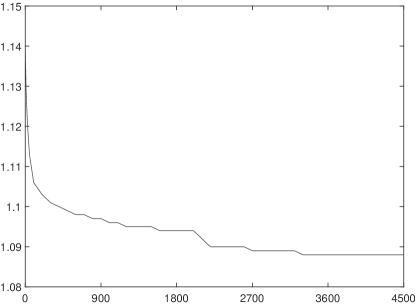
(a) Optimal value

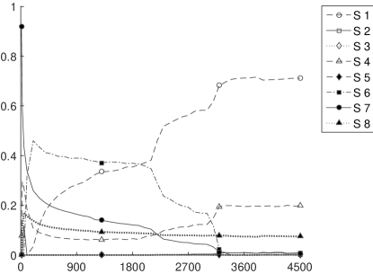
(b) Optimal solution

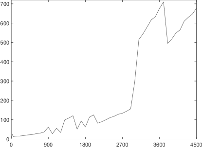
(c) Runnning time (in sec).

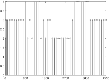
(d) Number of generated cuts.

Figure 1: Computational Results of Algorithm 1.

All experiments are conducted on a laptop with Intel Core i7 processor with 4 physical cores and hyper-threading on each core. The maximum frequency is 2.4 GHz with the boost at specific core up to 3.2 GHz. The maximum amount of RAM allowed for computation is 2 GB for each core. Step 3 in Algorithm 1 is coded using the optimization toolbox of Matlab R2015a, and step 5 is solved via the QCP solver of CPLEX 12.6. Both of the solvers work in parallel modes, which create $4$ clusters for Matlab and $4$ threads for CPLEX.

We run Algorithm 1 for case (i) with $\epsilon=0.1$. Figure 1 reports the optimal values and solutions, running times, and numbers of generated cuts when the degree $n$ of model BSD-P increases from 10 to 4500. Recall that the degree of model BSD-P is the degree of Bernstein polynomials approximating the set $\mathfrak{U}^{m}(\epsilon)$. Shown in Figures 1a and 1b, the optimal values and solutions fluctuate at the low degrees but become stable for the degrees larger than 3500.

The running time of Algorithm 1 is related to not only the degree but also the number of generated cuts. Note that the degree decides the number of decision variables in model BSD-P, and the number of generated cuts is the total iterations run by Algorithm 1. Figure 1c reflects the tendency that a longer running time is needed as the degree increases. However, the number of generated cuts is independent of the degree shown in Figure 1d. Particularly, Algorithm 1 generates 4 cuts when the degree varies in [3200, 3800], but there are only 3 cuts for the degree in [3900, 4500]. As the results, the running time reaches the peak, which is 710.11 seconds, for the degree is 3800, while it falls down to 494.94 seconds for the degree is 3900. Then the running time grows again to 647.01 seconds as the degree increases to 4500.

5.2 Effect Analysis of the RSD Constraint

We now analyze cases (i) - (iv) to test the effect of the RSD constraint (8b). The results are given in Figures 2 and 3. In this test, the degree of approximation is 4500, and the dominance level $\epsilon$ is adjusted in [0, 0.14]. In each case we divide this interval into three sub-intervals — weak region, mild region, and strong region — due to the strength of the RSD constraint (8b). In general, $\epsilon$ in the weak region is very small such that the optimal value and solutions of model (8) are identical to ones given by only using the reference utility function (i.e., $\epsilon=0$). Indeed, the RSD constraint (8b) has a limited impact on the performance of model (8) in the weak region. The strong region is opposite, for $\epsilon$ is rather large. The corresponding optimal value and solutions are very stable, and are indifferent to the reference utility function. In contrast, model (8) is sensitive to $\epsilon$ in the mild region. A small change on $\epsilon$ may incur completely different asset allocations in the portfolio.

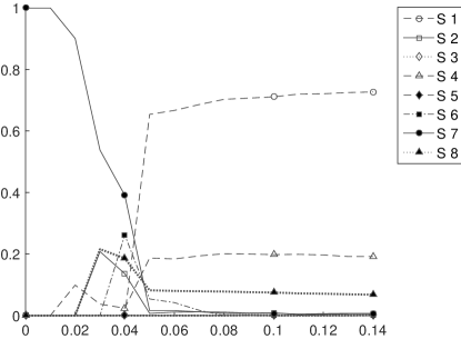
(a) Case (i).

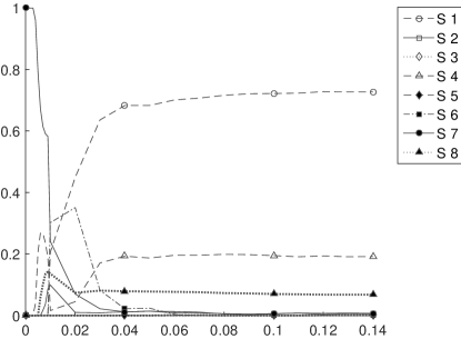
(b) Case (ii).

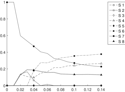
(c) Case (iii).

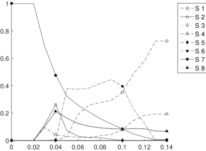
(d) Case (iv).

Figure 2: Impact of $\epsilon$ on the Optimal Asset Allocations for Cases (i)-(iv).

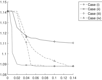
Figure 3: Expected Total Wealths of Cases (i)-(iv).

Case (i). In this case, the RSD constraint (8b) compares risky asset allocations with the benchmark $z^{Y_{1}}$, which only invests the risk-free asset S1. Shown in Figures 2a and 3, the weak region is [0, 0.01], the mild region is (0.01, 0.08), and the strong region is [0.08, 0.14]. Model (8) with $\epsilon$ in the weak region suggests that S7 obtain 100% of the total investment and yields the highest expected total wealth 1.141. As we increase $\epsilon$ to the mild region, the investment is diversified. For example, at $\epsilon=0.04$, the percentage of S7 in the portfolio dramatically decreases from 100% to 39.1%, while the percentages of S2, S4, S6, and S8 rise to 13.6%, 2.4%, 26.2%, and 18.6%, respectively. At $\epsilon=0.06$, S1 becomes crucial in the portfolio, owning 70.3% of the total investment and overwhelming S7 of which the percentage reduces to 1.2%. These results reflect the fact that, for satisfying the sufficient preference over the benchmark, the RSD constraint (8b) requires a large percentage of the total investment on the risk-free asset S1 to reduce the investment risk. As the effect of the RSD constraint (8b) is enhanced by increasing $\epsilon$, S1 gets more percentage until the strong region is reached. In the strong region, the investment is stable at (72.7%, 0.5%, 0.1%, 19.2%, 0%, 0%, 0.7%, 6.8%), which is very close to the solution (72.7%, 0.4%, 0%, 19.3%, 0%, 0%, 0.7%, 6.8%) suggested by the classical second order stochastic dominance ($\epsilon=1$). In addition, the decrease in the investment risk greatly reduces the expected total wealth, which rapidly decreases from 1.141 to 1.089 as $\epsilon$ changes from 0 to 0.05, and then slowly changes to 1.088. The over-conservativeness of stochastic dominance results in a very low yield, in comparison with the risk-free investment on S1 yielding the expected total wealth 1.078.

Case (ii). This case is designed to test the effect of the reference utility function in the RSD constraint (8b). We substitute the CARA utility function $u^{2}_{ref}$ for the CRRA utility function $u^{1}_{ref}$. In contrast, for the total wealth more than 1, $u^{2}_{ref}$ has a higher Arrow and Pratt’s measure of risk-aversion than $u^{1}_{ref}$, i.e.,

$$-\frac{(u^{2}_{ref})^{\prime\prime}(x)}{(u^{2}_{ref})^{\prime}(x)}=1>-\frac{(u^{1}_{ref})^{\prime\prime}(x)}{(u^{1}_{ref})^{\prime}(x)}=\frac{1}{x},\quad\text{for }x>1.$$

Hence, in this study, $u^{2}_{ref}$ characterizes stronger preference for low-risk investment than $u^{1}_{ref}$. It can be seen in Figures 2b and 3 that this substitution shrinks the weak region to [0, 0.003]. A subtle change on $\epsilon=0$ has a big impact on the investment proportion and total wealth. Analogous to case (i), the investment is diversified to hedge the risk in the mild region (0.003, 0.08). However, case (ii) has a much faster diversification rate. The asset allocation at $\epsilon=0.04$ is (68.3%, 1.2%, 0%, 19.3%, 0%, 2.2%, 1.2%, 7.9%), in which S1 has become a major invested asset, compared to 0% of the total investment on S1 in case (i). Also, this allocation is close to the stable solution, (72.7%, 0.5%, 0.1%, 19.2%, 0%, 0%, 0.7%, 6.8%), obtained in the strong region [0.08, 0.14]. Cases (i) and (ii) have the same asset allocation and total wealth in the strong region. This observation verifies that, for a sufficiently large $\epsilon$, the RSD constraint (8b) is indifferent to the reference utility function, and approaches to the classical stochastic dominance.

Case (iii). In this case the equal allocation benchmark $z^{Y_{2}}$ is substituted for the risk-free investment $z^{Y_{1}}$. Model (8) suggests a completely different investment policy without over-emphasizing the safety of investment. Shown in Figure 2c, S1 is not invested on, but S7 always obtains more than 22.8%. Figure 3 also indicates that the risky investment greatly raises the expected total wealth. In this case, the weak region is [0, 0.01] and the mild region is (0.01, 0.14]. Since the RSD constraint (8b) is ineffective in the weak region, the best policy is still 100% of the total investment on S7. As $\epsilon$ increases, the investment on S7 monotonically decreases, while S2, S4, S6, and S8 obtain more. The asset allocation is (0%, 6.3%, 0%, 9.7%, 0%, 18%, 47.2%, 18.7%) at $\epsilon=0.04$, and changes to (0%, 0%, 0%, 26.4%, 0%, 37.7%, 22.8%, 13%) at $\epsilon=0.14$. Different from case (i), there is not an overwhelming asset in case (iii), restricted by the benchmark $z^{Y_{2}}$ where every asset is equally treated.

Case (iv). This case tests the 3rd order RSD. As indicated by Proposition 1, case (iv) with the 3rd order RSD constraint (8b) is the relaxation of case (i). As the result, shown in Figures 2 and 3, the weak region is enlarged to [0, 0.02], the strong region shrinks to [0.13, 0.14], and the diversification rate is much slower in the widely spanned mild region. Moreover, the curve of the total wealth in case (iv) is always above the curve in case (i). At $\epsilon=0.04$, the asset allocation is (0%, 26.2%, 0%, 4.1%, 0%, 0.6%, 47.7%, 21.3%), in which case (iv) suggest 8.6% (= 47.7% - 39.1%) of the total investment on S7 more than case (i). At $\epsilon=0.06$, the allocation is (18.8%, 3.2%, 0%, 2.3%, 0%, 37.5%, 25.8%, 12.5%), in which S7 still gets more investment than S1 and S6 has the largest percentage.

5.3 Hannah’s Decision

We now discuss an investor’s desired dominance level in this portfolio problem. Recall that Table 1 lists the maximum dominance level of the lottery tickets $\bar{X}_{i}$, $i=1,\dots,5$, with respect to non-purchase option $\bar{Y}_{2}$. We request Hannah to choose the lottery tickets which she is not reluctant to purchase, and then evaluate her desired dominance level for risky investment. Similarly, we elicit Hannah’s desired dominance level for risk investment in case (i). $\bar{Y}_{2}$ does not take the risk-free interest into account. Hence, the total wealth $W_{1}$ yielded by only investing on asset S1 should be substituted for $\bar{Y}_{2}$ as the risk-free investment option. Table 3 gives the maximum dominance levels of lottery tickets $\bar{X}_{i}$ and $W_{1}$. Considering the risk-free interest leads to a little smaller levels in Table 3 than in Table 1.

Table 3: Maximum Dominance Levels of Lottery Tickets v.s. 100% of the Total Investment on S1

Lottery	Probability of Yield			Maximum Dominance Level
Ticket	$0	$2		$\mathcal{E}^{(2)}(\bar{X}_{i},W_{1};u^{1}_{ref})$
$\bar{X}_{1}$	1%	99%		0.112
$\bar{X}_{2}$	10%	90%		0.061
$\bar{X}_{3}$	25%	85%		0.037
$\bar{X}_{4}$	20%	80%		0.018
$\bar{X}_{5}$	25%	75%		0.003

Suppose that Hannah only picks up $\bar{X}_{1}$, and hence, her desired dominance level is 0.112. This level is in the strong region of case (i). Obviously, Hannah is a very cautious and discreet person, and thinks only $\bar{X}_{1}$ can almost dominate $W_{1}$. Figure 2a shows that her preferred asset allocation is (72%, 0.3%, 0%, 19.9%, 0%, 0%, 0.5%, 7.2%) and the expected total wealth is 1.088. Recall that the expected total wealth is 1.078 for the risk-free investment. If both $\bar{X}_{1}$ and $\bar{X}_{2}$ can be accepted, Hannah’s desired dominance level is 0.061. This level is in the mild region, and Hannah’s asset allocation is (66.7%, 1.1%, 0%, 18.4%, 0%, 4.2%, 1.6%, 8%), where the investment on S1 is reduced by 5.3% (= 72% - 66.7%), while the investment on S7 increases by 1.1% (= 1.6% - 0.5%). Correspondingly, the expected total wealth rises to 1.089. An appropriate assumption may be that Hannah also chooses $\bar{X}_{3}$ and her level is 0.037, at which the allocation is (0%, 13.6%, 0%, 2.4%, 0%, 26.2%, 39.1%, 18.6%). S7 gets 39.1% to the total investment for ensuring a reasonable expected total wealth as 1.111, and S2, S4, S6, and S8 are chosen in the diversification for hedging risk.

6 Conclusions

This paper has introduced a novel concept of reference-based almost stochastic dominance (RSD) and its application in risk-averse optimization problems. In the $\mathcal{L}_{2}$-normed space, we have specified a subset of the general class of risk-averse utility functions. This subset consists of nonparametric shape-preserving perturbations around a given reference utility function. The RSD represents a preference relation that a preferred uncertain prospect should have the larger expected utility over the perturbation subset. We have also defined the maximum dominance level, which quantifies the decision maker’s preference between alternative choices in the context of robustness.

We have proposed the RSD constrained stochastic optimization model and studied its solution method. An approximation approach based on Bernstein polynomials has been developed. This approach resorts to a cut-generation algorithm. We have discussed the asymptotic convergence of the optimal value and the set of optimal solutions obtained in this approach, and proved that the algorithm has finitely many iterations.

The portfolio optimization problem given by Dentcheva and Ruszczyński (2003) has been used to analyze the computational complexity of the approximation approach and to illustrate the effect of the RSD constraint. We have compared four cases with different benchmarks, reference utility functions, and dominance orders. In addition, we have discussed the impact of an investor’s desired dominance level on asset allocations.

Appendix A Asset Returns given in Dentcheva and Ruszczyński (2003)

Table 4: Asset Returns (in %) in Dentcheva and Ruszczyński (2003)

Year	A1	A2	A3	A4	A5	A6	A7	A8
1	7.5	-5.8	-14.8	-18.5	-30.2	2.3	-14.9	67.7
2	8.4	2.0	-26.5	-28.4	-33.8	0.2	-23.2	72.2
3	6.1	5.6	37.1	38.5	31.8	12.3	35.4	-24.0
4	5.2	17.5	23.6	26.6	28.0	15.6	2.5	-4.0
5	5.5	0.2	-7.4	-2.6	9.3	3.0	18.1	20.0
6	7.7	-1.8	6.4	9.3	14.6	1.2	32.6	29.5
7	10.9	-2.2	18.4	25.6	30.7	2.3	4.8	21.2
8	12.7	-5.3	32.3	33.7	36.7	3.1	22.6	29.6
9	15.6	0.3	-5.1	-3.7	-1.0	7.3	-2.3	-31.2
10	11.7	46.5	21.5	18.7	21.3	31.1	-1.9	8.4
11	9.2	-1.5	22.4	23.5	21.7	8.0	23.7	-12.8
12	10.3	15.9	6.1	3.0	-9.7	15.0	7.4	-17.5
13	8.0	36.6	31.6	32.6	33.3	21.3	56.2	0.6
14	6.3	30.9	18.6	16.1	8.6	15.6	69.4	21.6
15	6.1	-7.5	5.2	2.3	-4.1	2.3	24.6	24.4
16	7.1	8.6	16.5	17.9	16.5	7.6	28.3	-13.9
17	8.7	21.2	31.6	29.2	20.4	14.2	10.5	-2.3
18	8.0	5.4	-3.2	-6.2	-17.0	8.3	-23.4	-7.8
19	5.7	19.3	30.4	34.2	59.4	16.1	12.1	-4.2
20	3.6	7.9	7.6	9.0	17.4	7.6	-12.2	-7.4
21	3.1	21.7	10.0	11.3	16.2	11.0	32.6	14.6
22	4.5	-11.1	1.2	-0.1	-3.2	-3.5	7.8	-1.0

References

- Armbruster and Delage (2015) Armbruster, Benjamin., Erick. Delage. 2015. Decision making under uncertainty when preference information is incomplete. Management Science 61(1) 111–128.
- Bawa (1975) Bawa, Vijay. S. 1975. Optimal rules for ordering uncertain prospects. Journal of Financial Economics 2(1) 95–121.
- Ben-Tal and Nemirovski (1998) Ben-Tal, A., A. Nemirovski. 1998. Robust convex optimization. Mathematics of Operations Research 23(4) 769–805.
- Bertsimas et al. (2010) Bertsimas, D., X. V. Doan, K. Natarajan, C. Teo. 2010. Models for minimax stochastic linear optimization problems with risk aversion. Mathematics of Operations Research 35(3) 580–602.
- Bertsimas et al. (2004) Bertsimas, D., D. Pachamanova, M. Sim. 2004. Robust linear optimization under general norm. Operations Research Letters 32(6) 510–516.
- Boyd and Vandenberghe (2004) Boyd, S., L. Vandenberghe. 2004. Convex Optimization. Cambridge University Press.
- Brockett and Golden (1987) Brockett, Patrick. L., Linda. L. Golden. 1987. A class of utility functions containing all the common utility functions. Management Science 33(8) 955–964.
- Delage and Ye (2010) Delage, Erick., Yinyu. Ye. 2010. Distributionally robust optimization under moment uncertainty with application to data-driven problems. Operations Research 58(3) 595–612.
- Dentcheva et al. (2007) Dentcheva, D., R. Henrion, A. Ruszczyński. 2007. Stability and sensitivity of optimization problems with first order stochastic dominance constraints. SIAM J. Optim. 18(1) 322–337.
- Dentcheva and Ruszczyński (2003) Dentcheva, D., A. Ruszczyński. 2003. Optimization with stochastic dominance constraints. SIAM J. Optim. 14(2) 548–566.
- Dentcheva and Ruszczyński (2004) Dentcheva, D., A. Ruszczyński. 2004. Optimality and duality theory for stochastic optimization problems with nonlinear dominance constraints. Math. Programming 99 329–350.
- Dentcheva and Ruszczyński (2006) Dentcheva, D., A. Ruszczyński. 2006. Portfolio optimization with stochastic dominance constraints. Journal of Banking Finance 30 433–451.
- Drapkin and Schultz (2010) Drapkin, D., R. Schultz. 2010. An algorithm for stochastic programs with first-order dominance constraints induced by linear recourse. Discrete Applied Mathematics 158(4) 291–297.
- El Ghaoui and Lebret (1997) El Ghaoui, L., H. Lebret. 1997. Robust solutions to least-squares problems with uncertain data. SIAM Journal on Matrix Analysis and Applications 18 1035–1064.
- Farquhar (1984) Farquhar, Peter. H. 1984. Utility assessment methods. Management Science 30(11) 1283–1300.
- Hadar and Russell (1969) Hadar, J., W. Russell. 1969. Rules for ordering uncertain prospects. American Economic Review 59 25–34.
- Hanoch and Levy (1969) Hanoch, G., H. Levy. 1969. The efficiency analysis of choices involving risk. American Economic Review 36 335–346.
- Haskell and Jain (2015) Haskell, W. B., R. Jain. 2015. A convex analytic approach for risk-aware markov decision processes. SIAM Journal on Optimization and Control 53(3) 1569–1598.
- Hu et al. (2012) Hu, J., T. Homem-de-Mello, S Mehrotra. 2012. Sample average approximation of stochastic dominance constrained programs. Mathematical Programming 133(1-2) 171–201.
- Hu et al. (2013) Hu, J., T. Homem-de-Mello, S Mehrotra. 2013. Stochastically weighted stochastic dominance concepts with an application in capital budgeting. European Journal of Operational Research Publish online at http://dx.doi.org/10.1016/j.ejor.2013.08.007.
- Hu et al. (2015) Hu, J., J. Li, S. Mehortra. 2015. A data driven functionally robust approach for coordinating pricing and order quantity decisions with unknown demand function URL http://www.optimization-online.org/DB_HTML/2015/07/5016.html. IMSE, University of Michigan-Dearborn.
- Hu and Mehrotra (2015) Hu, J., S. Mehrotra. 2015. Robust decision making using a risk averse utility set with an application to portfolio optimization. IIE Transactions 47(4) 358–372.
- Karmarkar (1978) Karmarkar, Uday. S. 1978. Subjectively weighted utility: A descriptive extension of the expected utility model. Organizational Behavior and Human Performance 21(1) 61–72.
- Karoui and Meziou (2006) Karoui, N. E., A. Meziou. 2006. Constrained optimization with respect to stochastic dominance: Application to portfolio insurance. Mathematical Finance 16(1) 103–117.
- Lean et al. (2010) Lean, H. H., M. McAleerb, W. Wong. 2010. Market efficiency of oil spot and futures: A mean-variance and stochastic dominance approach. Energy Economics 32(5) 979–986.
- Leshno and Levy (2002) Leshno, Moshe., Haim. Levy. 2002. Preferred by ”all” and preferred by ”most” decision makers: Almost stochastic dominance. managment science 48(8) 1074–1085.
- Levy (2006) Levy, H. 2006. Stochastic Dominance : Investment Decision Making under Uncertainty. Springer, New York.
- Lizyayev and Ruszczyński (2012) Lizyayev, Andrey., Andrzej Ruszczyński. 2012. Tractable almost stochastic dominance. European Journal of Operational Research 218(2) 448–455.
- Luedtke (2008) Luedtke, J. 2008. New formulations for optimization under stochastic dominance constraints. SIAM Journal on Optimization 19(3) 1433–1450.
- Martein and Schaible (1987) Martein, L., S. Schaible. 1987. On solving a linear program with one quadratic constraint. Rivista di matematica per le scienze economiche e sociali 10(1-2) 75–90.
- Müller and Stoyan (2002) Müller, A., D. Stoyan. 2002. Comparison Methods for Stochastic Models and Risks. John Wiley & Sons, Chichester.
- Nie et al. (2012) Nie, Yu(Marco), Xing Wu, Tito Homem-de-Mello. 2012. Optimal path problems with second-order stochastic dominance constraints. Networks and Spatial Economics 12(4) 561–587.
- Noyan and Rudolf (2013) Noyan, N., G. Rudolf. 2013. Optimization with multivariate conditional value-at-risk constraints. Operational Research 61(4) 990–1013.
- Philips (2003) Philips, G. M. 2003. Interpolation and Approximation by Polynomials. Springer-Verlag, New York.
- Rivlin (1891) Rivlin, Theodore. J. 1891. An Introduction to the Approximation of Functions. Dover, New York.
- Roman et al. (2006) Roman, D., K. Darby-Dowman, G. Mitra. 2006. Portfolio construction based on stochastic dominance and target return distributions. Mathematical Programming 108(2–3) 541–569.
- Scarf (1958) Scarf, H. 1958. A min-max solution of an inventory problem. Studies in the Mathematical Theory of Inventory and Production, chap. 12. 201–209.
- Shaked and Shanthikumar (1994) Shaked, M., J. G. Shanthikumar. 1994. Stochastic Orders and their Applications. Academic Press, Boston.
- Shapiro et al. (2009) Shapiro, A., D. Dentcheva, A. Ruszczyński. 2009. Lectures on stochastic programming : Modeling and theory. SIAM.
- Shapiro and Ahmed (2004) Shapiro, Alexander., Shabbir. Ahmed. 2004. On a class of minimax stochastic programs. SIAM Journal on Optimization 14(4) 1237–1249.
- Sun and Xu (2014) Sun, H., H. Xu. 2014. Convergence analysis of stationary points in sample average approximation of stochastic programs with second order stochastic dominance constraints. Mathematical Programming 143(1-2) 31–59.
- van de Panne (1966) van de Panne, C. 1966. Programming with a quadratic constraint. Management Science 12(11) 798–815.
- Wakker and Deneffe (1996) Wakker, Peter., Daniel. Deneffe. 1996. Eliciting von Neumann-Morgenstern utilities when probabilities are distorted or unknown. Management Science 42(8) 1131–1150.
- Weber (1987) Weber, M. 1987. Decision making with incomplete information. European Journal of Operational Research 28(1) 44–57.