Abstract

Understanding the processes that give rise to quantitative measurements associated with molecular sequence data remains an important issue in statistical phylogenetics. Examples of such measurements include geographic coordinates in the context of phylogeography and phenotypic traits in the context of comparative studies. A popular approach is to model the evolution of continuously varying traits as a Brownian diffusion process acting on a phylogenetic tree. However, standard Brownian diffusion is quite restrictive and may not accurately characterize certain trait evolutionary processes. Here, we relax one of the major restrictions of standard Brownian diffusion by incorporating a nontrivial estimable drift into the process. We introduce a relaxed drift diffusion model for the evolution of multivariate continuously varying traits along a phylogenetic tree via Brownian diffusion with drift. Notably, the relaxed drift model accommodates branch-specific variation of drift rates while preserving model identifiability. Furthermore, our development of a computationally efficient dynamic programming approach to compute the data likelihood enables scaling of our method to large data sets frequently encountered in viral evolution. We implement the relaxed drift model in a Bayesian inference framework to simultaneously reconstruct the evolutionary histories of molecular sequence data and associated multivariate continuous trait data, and provide tools to visualize evolutionary reconstructions. We illustrate the utility of our approach in three viral examples. In the first two, we examine the spatiotemporal spread of HIV-1 in central Africa and West Nile virus in North America and show that a relaxed drift approach uncovers a clearer, more detailed picture of the dynamics of viral dispersal than standard Brownian diffusion. Finally, we study antigenic evolution in the context of HIV-1 resistance to three broadly neutralizing antibodies. Our analysis reveals evidence of a continuous drift at the HIV-1 population level towards enhanced resistance to neutralization by the VRC01 monoclonal antibody over the course of the epidemic.

1 Introduction

Phylogenetic inference has emerged as an important tool for understanding patterns of molecular sequence variation over time. Along with the increasing availability of molecular sequence data, there has been a growth of associated sources of information, such as spatial and phenotypic trait data, underscoring the need for integrated models of sequence and trait evolution on phylogenies, which promise to deliver more precise insights and increase opportunities for statistical hypothesis testing.

Much of the development of trait evolution models has been motivated by phylogenetic comparative approaches focusing on phenotypic and ecological traits. Traditional comparative methods assess the correlation between traits through standard regression models that assume taxa traits are generated independently by the same distribution. This assumption is obviously violated by taxa traits due to their shared ancestry. A proper understanding of patterns of correlation between traits can be achieved only by accounting for their shared evolutionary history (Felsenstein 1985; Harvey and Pagel 1991), and comparative methods focus on relating observed phenotype information to an evolutionary history.

Trait evolution has been tackled from another angle in phylogeographic approaches focusing on geographic locations rather than phenotypic traits. Evolutionary change is better understood when accounting for its geographic context, and phylogeographic inference methods aim to connect the evolutionary and spatial history of a population (Bloomquist et al. 2010). Phylogeographic techniques have allowed researchers to better understand the origin, spread, and dynamics of emerging infectious diseases. Examples include the human influenza A virus (Rambaut et al. 2008; Smith et al. 2009; Lemey et al. 2009b), rabies viruses (Biek et al. 2007; Seetahal et al. 2013), dengue virus (Bennett et al. 2010; Allicock et al. 2012) and hepatitis B virus (e.g. Mello et al. (2013)).

While methods for phenotypic and phylogeographic analyses are developed with different data in mind, they address similar situations and it is appropriate to speak more generally of trait evolution. Two key components required for modeling phylogenetic trait evolution are a method for incorporating phylogenetic information and a model of an evolutionary process on a phylogeny giving rise to the observed traits. Many popular approaches first reconstruct a phylogenetic tree and condition inferences pertaining to the trait evolution process on this fixed tree. However, computational advances, particularly in Markov chain Monte Carlo (MCMC) sampling techniques, have made it possible to control for phylogenetic uncertainty (as well as uncertainty in other important model parameters) through integrated models that jointly estimate parameters of interest (Huelsenbeck and Rannala 2003; Lemey et al. 2010).

The evolution of discrete traits has typically been modeled using continuous-time Markov chains (Felsenstein 1981; Pagel 1999; Lemey et al. 2009a), analogous to substitution models for molecular sequence characters. However, phenotypic and geographic traits are often continuously distributed, and while meaningful inferences may still be made partitioning the state space into finite parts, stochastic processes with continuous state spaces represent a more natural approach. A popular choice to model continous trait evolution along the lineages of a phylogenetic tree is Brownian diffusion (Felsenstein 1985). Lemey et al. (2010) and Pybus et al. (2012) have recently developed a computationally efficient Brownian diffusion model for evolution of multivariate traits in a Bayesian framework that integrates it with models for phylogenetic reconstruction and molecular evolution. Notably, their full probabilistic approach accounts for uncertainty in the phylogeny, demographic history and evolutionary parameters. Trait evolution is modeled as a multivariate time-scaled mixture of Brownian diffusion processes with a zero-mean displacement (or, in other words, neutral drift) along each branch of the possibly unknown phylogeny.

While adopting a mixture of Brownian diffusion processes is a popular and useful approach, it may not appropriately describe the evolutionary process in certain situations. Such scenarios are more realistically modeled by more sophisticated diffusion processes. There may, for example, be selection toward an optimal trait value. To address this phenomenon, there has been considerable development of mean-reverting Ornstein-Uhlenbeck process models for trait evolution, featuring a stochastic Brownian component along with a deterministic component (Hansen 1997; Butler and King 2004; Bartoszek et al. 2012).

Another trait evolutionary process inadequately modeled by standard Brownian diffusion is one characterized by directional trends. The need for relaxing the assumption of neutral drift is highlighted by a number of evolutionary scenarios in which there are apparent trends in the direction of variations, including antigenic drift in influenza (Bedford et al. 2014), the evolution of body mass in carnivores (Lartillot and Poujol 2011), and dispersal patterns of viral outbreaks (Pybus et al. 2012). To this end, we extend the Bayesian multivariate Brownian diffusion framework of Lemey et al. (2010) to allow for an unknown estimable nonzero drift vector for the mean displacement in a computationally efficient manner. While inclusion of a nontrivial drift represents a promising first step, a constant drift rate may not hold over an entire evolutionary history. We address this issue by presenting a flexible relaxed drift model that permits multiple drift rates on a phylogenetic tree. Importantly, we equip the model with machinery to infer the number of different drift rates supported by the data as well as the locations of rate changes.

We apply our relaxed drift diffusion methodology to three viral examples of clinical importance. In the first two examples, we illustrate our approach in a phylogeographic setting by investigating the spatial diffusion of HIV-1 in central Africa and the West Nile virus in North America. For the third example, we explore antigenic evolution in the context of enhanced resistance of HIV-1 to broadly neutralizing antibodes over the course of the epidemic. We employ model selection techniques to compare the nested drift-neutral, constant drift and relaxed drift Brownian diffusion models. We demonstrate a better fit by relaxing the restrictive drift-neutral assumption, and an improved ability to uncover and quantify key aspects of trait evolution dynamics.

2 Methods

We start by assuming we have a dataset of $N$ aligned molecular sequences $\textbf{X}=(\textbf{X}_{1},\dots,\textbf{X}_{N})$ along with $N$ associated $M$-dimensional, continuously varying traits $\textbf{Y}=(\textbf{Y}_{1},\dots,\textbf{Y}_{N})$. The sequence and trait data correspond to the tips of an unknown yet estimable phylogenetic tree $\tau$. Later we will discuss accounting for phylogenetic uncertainty, modeling the molecular evolution process giving rise to X and integrating it with a model for trait evolution. But first, we explore trait evolution on a fixed phylogeny via a diffusion process acting conditionally independently along its branches.

The $N$-tipped bifurcating phylogenetic tree $\tau$ is a graph with a set of vertices $\mathcal{V}=(\mathcal{V}_{1},\dots,\mathcal{V}_{2N-1})$ and edge weights $\mathcal{T}=(t_{1},\dots,t_{2N-2})$. The vertices correspond to nodes of the tree and, as the length of the tree $\tau$ is measured in units of time, $\mathcal{T}$ consists of times corresponding to branch lengths. Each external node $\mathcal{V}_{i}$ for $i=1,\dots,N$ is of degree 1, with one parent node $\mathcal{V}_{pa(i)}$ from within the internal or root nodes. Each internal node $\mathcal{V}_{i}$ for $i=N+1,\dots,2N-2$ is of degree 3 and the root node $\mathcal{V}_{2N-1}$ is of degree 2. An edge with weight $t_{i}$ connects $\mathcal{V}_{i}$ to $\mathcal{V}_{pa(i)}$, and we refer to this edge as branch $i$. In addition to the observed traits $\textbf{Y}_{1},\dots,\textbf{Y}_{N}$ at the external nodes, we posit for mathematical convenience unobserved traits $\textbf{Y}_{N+1},\dots,\textbf{Y}_{2N-1}$ at the internal nodes and root.

Brownian diffusion (also known as a Wiener process) is a continuous-time stochastic process originally developed to model the random motion of a physical particle (Brown 1828; Wiener 1958). Formally, a standard multivariate Brownian diffusion process $\textbf{W}(t)$ is characterized by the following properties: $\textbf{W}(0)=\textbf{0}$, the map $t\mapsto\textbf{W}(t)$ is almost surely continuous, $\textbf{W}(t)$ has independent increments and, for $0\leq s\leq t$, $\textbf{W}(t)-\textbf{W}(s)$ has a multivariate normal distribution with mean 0 and variance matrix $(t-s)\textbf{I}$.

Recent phylogenetic comparative methods (Vrancken et al. 2015; Cybis et al. 2015) aim to model the correlated evolution between multiple traits and, to this end, employ a correlated multivariate Brownian diffusion with displacement variance $(t-s)\textbf{P}^{-1}$. Here, P is an $M\times M$ infinitesimal precision matrix. The mean of 0 posits a neutral drift so that the traits do not evolve according to any systematic directional trend. Matrix P determines the intensity and correlation of the trait diffusion after controlling for shared evolutionary history.

The Brownian diffusion process along a phylogeny produces the observed traits by starting at the root node and proceeding down the branches of $\tau$. The displacement $\textbf{Y}_{i}-\textbf{Y}_{pa(i)}$ along a branch is multivariate normally distributed, centered at 0 with variance $t_{i}\textbf{P}^{-1}$ proportional to the length of the branch. Therefore, conditioning on the trait value $\textbf{Y}_{pa(i)}$ at the parent node, we have

$$\textbf{Y}_{i}|\textbf{Y}_{pa(i)}\sim N\left(\textbf{Y}_{pa(i)},t_{i}\textbf{P}^{-1}\right).$$ (1)

An extension that introduces branch-specific mixing parameters $\phi_{i}$ into the process that rescale $t_{i}\mapsto\phi_{i}t_{i}$ yields a mixture of Brownian processes and remains popular in phylogeography (Lemey et al. 2010).

2.1 Drift

To incorporate a directional trend, we adopt a multivariate correlated Brownian diffusion process with a non-neutral drift. In our drift diffusion process we replace the zero mean of the increment $\textbf{W}(t)-\textbf{W}(s)$ with the time-scaled mean vector $(t-s)\bm{\mu}$. The expected difference between the trait values of a descendant and its ancestor is determined by the overall drift vector $\bm{\mu}$ and the time elapsed between descendant and ancestor. This yields what we will call the constant drift model:

$$\textbf{Y}_{i}|\textbf{Y}_{pa(i)}\sim N\left(\textbf{Y}_{pa(i)}+t_{i}\bm{\mu},t_{i}\textbf{P}^{-1}\right).$$ (2)

While this approach is useful for modeling general directional trends, it is quite restrictive in that the drift $\bm{\mu}$ is fixed over the entire phylogeny. We can relax this assumption by introducing branch-specific drift vectors $\bm{\mu}_{i}$:

$$\textbf{Y}_{i}|\textbf{Y}_{pa(i)}\sim N\left(\textbf{Y}_{pa(i)}+t_{i}\bm{\mu}_{i},t_{i}\textbf{P}^{-1}\right)$$ (3)

for $i=1,\dots,2N-2$. We assign the root a conjugate prior

$$\textbf{Y}_{2N-1}\sim N\left(\bm{\mu}^{*},(\phi\textbf{P})^{-1}\right),$$ (4)

that is relatively uninformative for small values of $\phi$.

Conditioning on the trait value $\textbf{Y}_{2N-1}$ at the root of $\tau$, the joint distribution of observed traits $\textbf{Y}_{1},\dots,\textbf{Y}_{N}$ can be expressed as

$$\text{vec}\left[\textbf{Y}\right]|\left(\textbf{Y}_{2N-1},\textbf{P},\textbf{V}_{\tau},\bm{\mu}_{\tau}\right)\sim N\left(\textbf{Y}_{\text{root}}+\left(\textbf{T}\otimes\textbf{I}_{M}\right)\bm{\mu}_{\tau},\textbf{P}^{-1}\otimes\textbf{V}_{\tau}\right),$$ (5)

building on a similar construction for drift-neutral Brownian diffusion (Felsenstein 1973; Freckleton et al. 2002). Here, vec[Y] is the vectorization of the column vectors $\textbf{Y}_{1},\dots,\textbf{Y}_{N}$, while $\textbf{I}_{M}$ is an $M\times M$ identity matrix, and $\otimes$ is the Kronecker product. $\textbf{Y}_{\text{root}}$ is the $NM\times 1$ vector $(\textbf{Y}^{t}_{2N-1},\dots,\textbf{Y}^{t}_{2N-1})^{t}$, and $\bm{\mu}_{\tau}$ is the $(2N-2)M\times 1$ drift rate vector $(\bm{\mu}^{t}_{1},\dots,\bm{\mu}^{t}_{2N-2})^{t}$. The $N\times N$ variance matrix $\textbf{V}_{\tau}$ is a deterministic function of $\tau$ and represents the contribution of the phylogenetic tree to the covariance structure. Its diagonal entries $V_{ii}$ are equal to the distance in time between the tip $\mathcal{V}_{i}$ and the root node $\mathcal{V}_{2N-1}$, and off-diagonal entries $V_{ij}$ correspond to the distance in time between the root node $\mathcal{V}_{2N-1}$ and the most recent common ancestor of tips $\mathcal{V}_{i}$ and $\mathcal{V}_{j}$. Finally, the $N\times(2N-2)$ matrix T is defined as follows: $T_{ij}=t_{j}$, the length of branch $j$, if branch $j$ is part of the path from the external node $i$ to the root, and $T_{ij}=0$ otherwise.

Our development thus far clarifies some important issues. First, while it is tempting to model a unique drift rate on each branch, not all $\bm{\mu}_{i}$ are uniquely identifiable in the likelihood (5). Care must be taken to impose necessary restrictions to ensure identifiability while still permitting sufficient drift rate variation, and we discuss an approach to achieve this in section 2.3. Second, the variance matrix $\textbf{P}^{-1}\otimes\textbf{V}_{\tau}$ in (5) suggests a computational order of $\mathcal{O}(N^{3}M^{3})$ to evaluate the density. Repeated evaluation of (5) is necessary for numerical integration in Bayesian modeling, and viral data sets may encompass thousands of sequences. Fortunately, Pybus et al. (2012) demonstrate that phylogenetic Brownian diffusion likelihoods can be evaluated in computational order $\mathcal{O}(NM^{2})$ by modeling in terms of the precision matrix P (as opposed to the variance) and adopting a dynamic programming approach. In section 2.2, we present an adaptation of their algorithm for our drift diffusion likelihood.

2.2 Multivariate Trait Peeling

Under our Brownian drift diffusion process, the joint distribution of all traits is straightforwardly expressed as the product

$$P(\textbf{Y}_{1},\dots,\textbf{Y}_{2N-1}|\tau,\textbf{P},\bm{\mu},\phi)=\left(\prod_{i=1}^{2N-2}P(\textbf{Y}_{i}|\textbf{Y}_{pa(i)},\textbf{P},t_{i},\bm{\mu}_{i})\right)P(\textbf{Y}_{2N-1}|\textbf{P},\bm{\mu}^{*},\phi),$$ (6)

where $\bm{\mu}=(\bm{\mu}_{1},\dots,\bm{\mu}_{2N-2},\bm{\mu}^{*})$. The density of the observed traits can then be obtained by integrating over all possible realizations of the unobserved traits at the root and internal nodes. We adopt a dynamic programming approach that is analogous to Felsenstein’s pruning method (Felsenstein 1981) and has been employed for drift-neutral Brownian diffusion likelihoods (Pybus et al. 2012; Vrancken et al. 2015; Cybis et al. 2015) .

We wish to compute the density

$$P(\textbf{Y}_{1},\dots,\textbf{Y}_{N}) =\int\cdots\int P(\textbf{Y}_{1},\dots,\textbf{Y}_{2N-1})d\textbf{Y}_{N+1}\dots d\textbf{Y}_{2N-1}$$ (7)

$$=\int\cdots\int\left(\prod_{i=1}^{2N-2}P(\textbf{Y}_{i}|\textbf{Y}_{pa(i)})\right)P(\textbf{Y}_{2N-1})d\textbf{Y}_{N+1}\dots d\textbf{Y}_{2N-1}.$$ (8)

We have omitted dependence on the parameters $\tau,\textbf{P},\bm{\mu}_{1},\dots,\bm{\mu}_{2N-2},\bm{\mu}*$ and $\phi$ from the notation for the sake of clarity. The integration proceeds in a postorder traversal integrating out one internal node trait at a time. Let $\{\textbf{Y}_{i}\}$ denote the set of observed trait values descendant from and including the node $V_{i}$, and suppose $pa(i)=pa(j)=k$. Our traversal requires computing integrals of the form

$$P(\{\textbf{Y}_{k}\}|\textbf{Y}_{pa(k)})=\int P(\{\textbf{Y}_{i}\}|\textbf{Y}_{k})P(\{\textbf{Y}_{j}\}|\textbf{Y}_{k})P(\textbf{Y}_{k}|\textbf{Y}_{pa(k)})d\textbf{Y}_{k}.$$ (9)

Because the integrand is proportional to a multivariate normal density, it suffices to keep track of partial mean vectors $\textbf{m}_{k}$, partial precision scalars $p_{k}$ and normalizing constants $\rho_{k}$.

Let MVN(.;$\bm{\kappa}$,$\bm{\Lambda}$) denote a multivariate normal probability density function with mean $\bm{\kappa}$ and precision $\bm{\Lambda}$. We can rewrite conditional densities to facilitate integration with respect to the trait at the parent node:

$$P(\textbf{Y}_{i}|\textbf{Y}_{k}) = \mbox{MVN}\left(\textbf{Y}_{i};t_{i}\bm{\mu}_{i}+\textbf{Y}_{k},\frac{1}{t_{i}}\textbf{P}\right)$$ (10)

$$= \mbox{MVN}\left(\textbf{Y}_{i}-t_{i}\bm{\mu}_{i};\textbf{Y}_{k},\frac{1}{t_{i}}\textbf{P}\right).$$ (11)

For $i=1,\dots,N$, set normalizing constant $\rho_{i}=1$, partial mean

$$\textbf{m}_{i}=\textbf{Y}_{i}-t_{i}\bm{\mu}_{i}$$ (12)

and partial precision

$$p_{i}=\frac{1}{t_{i}}.$$ (13)

Then

$$P(\{\textbf{Y}_{i}\}|\textbf{Y}_{k})P(\{\textbf{Y}_{j}\}|\textbf{Y}_{k}) = \rho_{i}\rho_{j}\times\mbox{MVN}(\textbf{m}_{i};\textbf{Y}_{k},p_{i}\textbf{P})\times$$

$$\quad\quad\mbox{MVN}(\textbf{m}_{j};\textbf{Y}_{k},p_{j}\textbf{P})$$

$$= \rho_{k}\times\mbox{MVN}(\textbf{Y}_{k};\textbf{m}^{*}_{k},(p_{i}+p_{j})\textbf{P})$$ (15)

where partial unshifted mean

$$\textbf{m}^{*}_{k}=\frac{p_{i}\textbf{m}_{i}+p_{j}\textbf{m}_{j}}{p_{i}+p_{j}},$$ (16)

and normalizing constant

$$\rho_{k}=\rho_{i}\rho_{j}\left(\frac{p_{i}p_{j}}{2\pi(p_{i}+p_{j})}\right)^{d/2}|\textbf{P}|^{1/2}\frac{\exp\left[-\frac{p_{i}}{2}\textbf{m}_{i}^{\prime}\textbf{P}\textbf{m}_{i}-\frac{p_{j}}{2}\textbf{m}_{j}^{\prime}\textbf{P}\textbf{m}_{j}\right]}{\exp\left[-\frac{p_{i}+p_{j}}{2}\textbf{m}^{*^{\prime}}_{k}\textbf{P}\textbf{m}^{*}_{k}\right]}.$$ (17)

Multiplying by $P(\textbf{Y}_{k}|\textbf{Y}_{pa(k)})$ and integrating with respect to $\textbf{Y}_{k}$, we get

$$P(\{\textbf{Y}_{k}\}|\textbf{Y}_{pa(k)}) = \int P(\{\textbf{Y}_{i}\}|\textbf{Y}_{k})P(\{\textbf{Y}_{j}\}|\textbf{Y}_{k})P(\textbf{Y}_{k}|\textbf{Y}_{pa(k)})d\textbf{Y}_{k}$$ (18)

$$= \rho_{k}\times\mbox{MVN}(\textbf{Y}_{pa(k)};\textbf{m}_{k},p_{k}\textbf{P}),$$ (19)

where

$$\textbf{m}_{k}=\textbf{m}^{*}_{k}-t_{k}\bm{\mu}_{k},$$ (20)

and

$$p_{k}=\frac{1}{t_{k}+\frac{1}{p_{i}+p_{j}}}.$$ (21)

Integrating out all internal node traits yields

$$P(\textbf{Y}_{1},\dots,\textbf{Y}_{N}|\textbf{Y}_{2N-1})=\rho_{2N-1}\times\mbox{MVN}(\textbf{Y}_{2N-1};\textbf{m}^{*}_{2N-1},(p_{2N-2}+p_{2N-3})\textbf{P}).$$ (22)

For the final step, we multiply by the conjugate root prior and integrate:

$$P(\textbf{Y}_{1},\dots,\textbf{Y}_{N}) = \int P(\textbf{Y}_{1},\dots,\textbf{Y}_{N}|\textbf{Y}_{2N-1})P(\textbf{Y}_{2N-1})d\textbf{Y}_{2N-1}$$ (23)

$$= \rho_{2N-1}\mbox{MVN}(\textbf{m}^{*}_{2N-1};\bm{\mu}^{*},p_{2N-1}\textbf{P}),$$ (24)

where

$$p_{2N-1}=\frac{(p_{2N-2}+p_{2N-3})\phi}{p_{2N-2}+p_{2N-3}+\phi}.$$ (25)

In practice, the algorithm visits each node in the phylogeny once and computes partial unshifted means $\textbf{m}^{*}_{k}$, partial means $\textbf{m}_{k}$, partial precisions $p_{k}$, and normalizing constants $\rho_{k}$.

2.3 Identifiability and Relaxed Drift

Ideally, we would like to model a unique drift rate $\bm{\mu}_{i}$ on each branch $i$ of the phylogenetic tree. However, such lax assumptions open the door to misleading inferences. Adopting the notation of section 2.1, there can exist distinct drift rate vectors $\bm{\mu}_{\tau}\neq\bm{\mu}^{*}_{\tau}$ such that

$$\left(\textbf{T}\otimes\textbf{I}_{M}\right)\bm{\mu}_{\tau}=\left(\textbf{T}\otimes\textbf{I}_{M}\right)\bm{\mu}^{*}_{\tau},$$ (26)

yielding identical trait likelihoods (5). The lack of model identifiability presents an obstacle to uncovering the “true” values of the drift rates that characterize the trait evolution process.

We propose a relaxed drift model that allows for drift rate variation along a phylogenetic tree while maintaining model identifiability. This is achieved by having branches inherit drift rates from ancestral branches by default, but allowing a random number of specific types of rate changes to occur along the tree. We describe the model here and refer readers to the Appendix for a detailed argument establishing identifiability.

We begin at the unobserved branch leading to the root, or most recent common ancestor (MRCA), of the phylogenetic tree $\tau$ and associate with it the drift $\bm{\mu}_{\text{\tiny MRCA}}$. Then the two branches emanating from the root node either both inherit the drift rate $\bm{\mu}_{\text{\tiny MRCA}}$, or a rate change occurs and one branch receives a new rate while the other branch assumes the rate $\bm{\mu}_{\text{\tiny MRCA}}$. Similarly, whenever a branch splits into two anywhere in $\tau$, either both child branches assume the same drift rate as the parent branch, or one child branch takes on a new value while the other inherits its drift from the parent branch. Both child branches taking on different drift rates than the parent branch is not permitted.

Importantly, rather than fix the type of drift rate transfer that occurs at a given node, we estimate it from the data. The benefits of this choice are twofold. First, a rate change is not forced when the data do not suggest a need for one. Unnecessarily imposing a large number of unique drift rates to be inferred from limited data can lead to high variance estimates. Second, in the event of a rate change occurring at a node, only one of the two child branches can assume a new drift rate. We let the data determine which of the child branches assumes the new rate. The data may support new rates on both child branches. While our model may seem too restrictive to accommodate such a scenario at first glance, we are able to infer the relative support for each child, and it is reflected in the posterior distribution in terms of the probabilities of the two types of changes. Thus summaries of the posterior distribution can capture the true nature of drift rate variation in spite of the identifiability restrictions.

It is important to handle the initial drift rate $\bm{\mu}_{\text{\tiny MRCA}}$ with care. One option is to estimate $\bm{\mu}_{\text{\tiny MRCA}}$ from the data just as with all other drift rates. However, such a choice may not be ideal for data sets that exhibit relatively long periods of divergence from the MRCA to the sampling times. There is generally more information about diffusion dynamics during time periods overlapping with or close to sampling times. Likewise, the further removed the MRCA is from sampling times, the less information there is about $\bm{\mu}_{\text{\tiny MRCA}}$ and other drift rates near the MRCA. Because of the interconnectedness of branch drift rates in the relaxed model, estimates of $\bm{\mu}_{\text{\tiny MRCA}}$ and neighboring drift rates under such circumstances may primarily reflect information about drift rates on branches near sampling times. To mitigate misleading inferences of drift near the MRCA, we can adopt an initial drift $\bm{\mu}_{\text{\tiny MRCA}}=0$ and still interprete changes in drift rates across the tree.

To parameterize the model, we associate a ternary variable $\bm{\delta}_{k}$ with each internal node $k$ specifying how it passes on its drift rate to its child nodes. Suppose node $k$ has left child node $i$ and right child node $j$. If $\bm{\delta}_{k}=-1$, then $\bm{\mu}_{i}=\bm{\mu}_{k}$ and node $j$ assumes a new rate $\bm{\mu}_{j}=\bm{\mu}_{k}+\bm{\alpha}_{j}$. If $\bm{\delta}_{k}=1$, then node $i$ assumes a new rate $\bm{\mu}_{i}=\bm{\mu}_{k}+\bm{\alpha}_{i}$ while $\bm{\mu}_{j}=\bm{\mu}_{k}$. If $\bm{\delta}_{k}=0$, then no drift rate changes occur and $\bm{\mu}_{k}=\bm{\mu}_{i}=\bm{\mu}_{j}$. To map the ternary $\bm{\delta}_{k}$ variables to binary indicators $\bm{\gamma}_{i}$ of rate changes for child branches, we define

$$\bm{\gamma}_{i}=\frac{1+\bm{\delta}_{k}}{2}|\bm{\delta}_{k}|,$$ (27)

and

$$\bm{\gamma}_{j}=\frac{1-\bm{\delta}_{k}}{2}|\bm{\delta}_{k}|.$$ (28)

Thus

$$\bm{\mu}_{i}=\bm{\mu}_{pa(i)}+\bm{\gamma}_{i}\bm{\alpha}_{i},$$ (29)

for $i=1,\dots,2N-2$. Working with the binary $\bm{\gamma}_{i}$ eases our understanding of the MCMC procedure to infer drift rate changes, discussed below. However, we parameterize the model in terms of the ternary $\bm{\delta}_{k}$ to facilitate enforcement of the model restrictions.

Of particular interest is the random number $K\in{0,\dots,N-1}$ of rate changes that occur in $\tau$. We can write $K$ in terms of the $\bm{\delta}_{i}$,

$$K=\sum_{i=N+1}^{2N-1}|\bm{\delta}_{i}|,$$ (30)

and it provides us with a natural way to think of the vector $\bm{\delta}=(\bm{\delta}_{N+1},\dots,\bm{\delta}_{2N-1})$. For example, we can express our prior beliefs about $\bm{\delta}$ in terms of $K$. A popular prior for count data is the Poisson distribution

$$K\sim\mbox{Poisson}(\lambda).$$ (31)

Here, $\lambda$ is the expected number of rate changes in $\tau$. In our analyses, we set $\lambda=\log(2)$, which places 50$\%$ prior probability on the hypothesis of no rate changes.

In order to infer the nature of the drift rate transitions that occur at the nodes of the phylogenetic tree, we borrow ideas from Bayesian stochastic search variable selection (BSSVS) (George and McCulloch 1993; Kuo and Mallick 1998; Chipman et al. 2001). BSSVS is typically applied to model selection problems in a linear regression setting. In this framework, we begin with a large number $P$ of potential predictors $\textbf{X}_{1},\dots,\textbf{X}_{P}$ and seek to determine which of them associate linearly with an $N$-dimensional outcome Y. The full model with all predictors is

$$\textbf{Y}=\textbf{X}_{1}\bm{\beta}_{1}+\dots+\textbf{X}_{P}\bm{\beta}_{P}+\bm{\epsilon},$$ (32)

where the $\bm{\beta}_{i}$ are regression coefficients and $\bm{\epsilon}$ is a vector of normally distributed error terms with mean 0. When a particular $\bm{\beta}_{i}$ is determined to differ significantly from 0, the corresponding $\textbf{X}_{i}$ helps predict Y. If not, $\textbf{X}_{i}$ contributes little additional information and is fit to be removed from the model by forcing $\bm{\beta}_{i}=0$. Predictors may be highly correlated, and deterministic model selection strategies tend not to find the optimal set of predictors without exploring all possible subsets. There exist $2^{P}$ such subsets, so exploring all of them is computationally unfeasible in general and fails completely for $P>N$.

BSSVS efficiently explores the possible subsets of model predictors by augmenting the model state space with a vector $\bm{\delta}=(\bm{\delta}_{1},\dots,\bm{\delta}_{P})$ of binary indicator variables that dictate which predictors to include. The indicators $\bm{\delta}_{i}$ impose a prior on the regression coefficients $\bm{\beta}=(\bm{\beta}_{1},\dots,\bm{\beta}_{P})$ with mean 0 and variance proportional to a $P\times P$ diagonal matrix with its diagonal equal to $\bm{\delta}$. If $\bm{\delta}_{i}=0$, then the prior variance on $\bm{\beta}_{i}$ shrinks to 0 and forces $\bm{\beta}_{i}=0$ in the posterior. The joint space $(\bm{\beta},\bm{\delta})$ is explored simultaneously through MCMC.

We apply BSSVS in our relaxed drift setting to determine the types of drift rate transfers that occur. We achieve this by exploring the joint space $(\bm{\alpha},\bm{\delta})$ of rate differences between parent and child branches, and ternary rate change indicators. The $\bm{\delta}_{k}$ map to binary indicators $\bm{\gamma}_{i}$, as shown in (27) and (28). We assume that drift rate differences $\bm{\alpha}_{i}=\bm{\mu}_{i}-\bm{\mu}_{pa(i)}$ are $\it{a}$ $\it{priori}$ independent and normally distributed,

$$\bm{\alpha}_{i}\sim N(\textbf{0},\bm{\gamma}_{i}\sigma^{2}\textbf{I}).$$ (33)

If $\bm{\gamma}_{i}=0$, then the prior variance $\sigma^{2}$ on the components of $\bm{\alpha}_{i}$ shrinks to 0. This forces $\bm{\alpha}_{i}=\textbf{0}$, and hence $\bm{\mu}_{i}=\bm{\mu}_{pa(i)}$, in the posterior.

We complete our drift diffusion model specification by assigning the precision matrix P a Wishart prior with, say, degrees of freedom $v$ and scale matrix V. Importantly, the Wishart distribution is conjugate to the observed trait likelihood. Indeed, invoking the notation for partial means and precisions from section 2.2, the posterior

$$P(\textbf{P}|\textbf{Y}_{1},\dots,\textbf{Y}_{N})\propto P(\textbf{Y}_{1},\dots,\textbf{Y}_{N}|\textbf{P})P(\textbf{P})$$ (34)

has a Wishart distribution with $N+v$ degrees of freedom and scale matrix

$$\Biggl{(}\textbf{V}^{-1}+p_{2N-1}(\textbf{m}^{*}_{2N-1}-\bm{\mu}^{*})(\textbf{m}^{*}_{2N-1}-\bm{\mu}^{*})^{\prime}\\ +\sum_{k=N+1}^{2N-1}[p_{i}\textbf{m}_{i}\textbf{m}^{\prime}_{i}+p_{j}\textbf{m}_{j}\textbf{m}^{\prime}_{j}-(p_{i}+p_{j})\textbf{m}^{*}_{k}\textbf{m}^{*^{\prime}}_{k}]\Biggr{)}^{-1}.$$ (35)

Lemey et al. (2010) exploit a similar conjugacy to construct an efficient Gibbs sampler for P, and our adoption of the Wishart prior conveniently allows us to extend use of the sampler to our model that now includes a relaxed drift process.

2.4 Joint Modeling and Inference

A major strength of our Bayesian framework is that it jointly models sequence and trait evolution. Adopting a standard phylogenetic approach, we assume the sequence data X arise from a continuous-time Markov chain (CTMC) model for character evolution acting along the unobserved phylogenetic tree $\tau$. The CTMC is characterized by a vector Q of mutation parameters that may include, for instance, relative exchange rates among characters, an overall rate multiplier and across-site variation specifications. The traits Y arise from a Brownian drift diffusion process acting on $\tau$, governed by parameters $\bm{\Lambda}$. A crucial assumption is that the processes giving rise to the observed sequences and traits are conditionally independent given the phylogenetic tree $\tau$:

$$P(\textbf{X},\textbf{Y}|\tau,\textbf{Q},\bm{\Lambda})=P(\textbf{X}|\tau,\textbf{Q})P(\textbf{Y}|\tau,\bm{\Lambda}),$$ (36)

enabling us to write the joint model posterior distribution as

$$P(\tau,\textbf{Q},\bm{\Lambda}|\textbf{X},\textbf{Y})\propto P(\textbf{X}|\tau,\textbf{Q})P(\textbf{Y}|\tau,\bm{\Lambda})P(\tau)P(\textbf{Q})P(\bm{\Lambda}).$$ (37)

We implement the joint model by integrating our drift diffusion framework for trait evolution into the Bayesian Evolutionary Analysis Sampling Trees (BEAST) software package (Drummond et al. 2012). BEAST provides an array of efficient methods for Bayesian phylogenetic inference, particularly to estimate phylogenies and model molecular sequence evolution. For the phylogeny $\tau$, we choose from flexible coalescent-based priors that do not make strong $\it{a}$ $\it{priori}$ assumptions about the population history (Minin et al. 2008; Gill et al. 2013). For sequence evolution, we have access to a range of classic substitution models (Kimura 1980; Felsenstein 1981; Hasegawa et al. 1985), gamma-distributed rate heterogeneity among sites (Yang 1994), and strict and relaxed molecular clock models for branch rates (Drummond et al. 2006).

Estimation of the full joint posterior (37) is achieved through MCMC sampling (Metropolis et al. 1953; Hastings 1970). We employ standard Metropolis-Hastings transition kernels available in BEAST to integrate over the parameter spaces of Q and $\tau$. To sample realizations of the drift diffusion precision matrix P, we adapt a Gibbs sampler developed for drift-neutral Brownian diffusion (Lemey et al. 2010). For the relaxed drift model, we need transition kernels to explore the space $(\bm{\alpha},\bm{\delta})$ of branch rate differences and ternary rate change indicators. We propose new rate differences $\bm{\alpha}^{*}_{i}$ component-wise through a random walk transition kernel that adds random values within a specified window size to the current $\bm{\alpha}_{i}$.

For $\bm{\delta}$, we implement a trit-flip transition kernel that chooses one of the $N-1$ ternary indicators $\bm{\delta}_{k}$ uniformly at random and proposes a new state $\bm{\delta}^{*}_{k}$ assuming one of the two possible values not equal to $\bm{\delta}_{k}$ with equal probability. For example, if $\bm{\delta}_{k}=0$, then

$$\bm{\delta}^{*}_{k}=\begin{cases}-1&\text{with probability }\frac{1}{2}\\ 1&\text{with probability }\frac{1}{2}.\end{cases}$$ (38)

We have parameterized our prior on $\bm{\delta}$ in terms of the number $K$ of rate changes, and this parameterization should be retained for the transition kernel in order to ensure the correct Metropolis-Hastings proposal ratio (Drummond and Suchard 2010). A proposed increase in rate changes occurs when we choose a $\bm{\delta}_{k}$ with value 0, so

$$q(K^{*}=K+1|K)=\frac{N-1-K}{N-1}.$$ (39)

If we choose a $\bm{\delta}_{k}$ with a nonzero value, we propose the other nonzero value with probability 0.5 (corresponding to $K^{*}=K$), and we propose 0 with probability 0.5 (which means a decrease in rate changes, $K^{*}=K-1$). Therefore

$$q(K^{*}=K|K)=q(K^{*}=K-1|K)=\frac{1}{2}\frac{K}{N-1}.$$ (40)

These calculations yield the following proposal ratio for $K$:

$$\frac{q(K|K^{*})}{q(K^{*}|K)}=\begin{cases}\frac{1}{2}\frac{K+1}{N-1-K}&\text{if }K^{*}=K+1\\ 1&\text{if }K^{*}=K\\ \frac{2(N-K)}{K}&\text{if }K^{*}=K-1.\end{cases}$$ (41)

In addition to the parameters characterizing the trait and sequence evolution processes, we may wish to make inferences about the posterior distribution of traits at the root and internal nodes, or at any arbitrary time point in the past. We equip BEAST with the ability to generate posterior trait realizations at these nodes by implementing a preorder, tree-traversal algorithm.

A natural choice to summarize the results of a Bayesian phylogenetic analysis is a maximum clade credibility (MCC) tree. To form an MCC tree, the posterior sample of trees is examined to determine posterior clade probabilities, and the tree with the maximum product of posterior clade probabilities is the MCC tree. The branches and nodes of MCC trees can be annotated with inferred drift rates and trait values, along with other quantities of interest. Annotated MCC trees can be summarised using TreeAnnotator, available as part of the BEAST distribution, and visualized using FigTree (http://tree.bio.ed.ac.uk/software/figtree/).

2.5 Model Selection

We can formally compare the constant and relaxed drift diffusion models through Bayes factors (BFs). A Bayes factor (Jeffreys 1935, 1961) compares the fit of two models, $M_{1}$ and $M_{0}$, to observed data $(\textbf{X},\textbf{Y})$ by taking the ratio of marginal likelihoods:

$$BF_{10}=\frac{P(\textbf{X},\textbf{Y}|M_{1})}{P(\textbf{X},\textbf{Y}|M_{0})}=\frac{P(M_{1}|\textbf{X},\textbf{Y})}{P(M_{0}|\textbf{X},\textbf{Y})}\left/\frac{P(M_{1})}{P(M_{0})}\right..$$ (42)

$BF_{10}$ quantifies the evidence in favor of model $M_{1}$ over $M_{0}$. Kass and Raftery (1995) provide guidelines for assessing the strength of the evidence against $M_{0}$: BFs between 1 and 3 are not worth more than a bare mention, while values between 3 and 20 are considered positive evidence against $M_{0}$. BFs in the ranges 20-150 and $>$150 are considered to be strong and very strong evidence against $M_{0}$, respectively.

Evaluation of Bayes factors has become a popular approach to model selection in Bayesian phylogenetics (Sinsheimer et al. 1996; Suchard et al. 2001, 2005). Marginal likelihood estimation can be quite difficult in a phylogenetic context, and stepping-stone sampling estimators have been implemented to address this (Baele et al. 2012, 2013; Baele and Lemey 2013). Following the approach of Drummond and Suchard (2010), however, we are able to straightforwardly compute the Bayes factor $BF_{C}$ supporting the constant drift model $M_{C}$ over the relaxed drift model $M_{R}$. The model $M_{C}$ is nested within the more general model $M_{R}$ and occurs when $K=0$. This enables us to write

$$BF_{C} = \frac{P(\textbf{X},\textbf{Y}|M_{C})}{P(\textbf{X},\textbf{Y}|M_{R})}=\frac{P(M_{C}|\textbf{X},\textbf{Y})}{P(M_{R}|\textbf{X},\textbf{Y})}\left/\frac{P(M_{C})}{P(M_{R})}\right.$$ (43)

$$= \frac{P(K=0|\textbf{X},\textbf{Y},M_{R})}{1-P(K=0|\textbf{X},\textbf{Y},M_{R})}\left/\frac{P(K=0|M_{R})}{1-P(K=0|M_{R})}\right.,$$ (44)

requiring only our prior probability of no rate changes under the relaxed drift model, and the posterior probability of zero rate changes.

3 The Spread of HIV-1 in Central Africa

Faria et al. (2014) explore the early spatial expansion and epidemic dynamics of HIV-1 in central Africa by analyzing sequence data sampled from countries in the Congo River basin. The authors employ a discrete phylogeographic inference framework (Lemey et al. 2009a) and show that the pandemic likely originated in Kinshasa (in what is now the Democratic Republic of Congo) in the 1920s. Furthermore, viral spread to other population centers in sub-Saharan Africa was aided by a combination of factors, including strong railway networks, urban growth, and changes in sexual behavior.

We follow up the analysis of Faria et al. (2014) by applying our continuous drift diffusion approach to one of the data sets analysed in this study. The data set consists of HIV-1 sequences sampled between 1985-2004 from the Democratic Republic of Congo and the Republic of Congo and includes 96 sequences from Kinshasa (Kalish et al. 2004; Vidal et al. 2000, 2005; Yang et al. 2005), 96 sequences from Mbuji-Mayi (Vidal et al. 2000, 2005), 96 from Brazzaville (Bikandou et al. 2004; Niama et al. 2006), 76 from Lubumbashi (Vidal et al. 2005), 33 from Bwamanda (Vidal et al. 2000), 24 from Likasi (Kita et al. 2004), 23 from Kisangani (Vidal et al. 2005), and 22 sequences from Pointe-Noire (Bikandou et al. 2000). We reconstruct the spatial dynamics under drift-neutral, constant drift, and relaxed drift Brownian diffusion on a maximum clade credibility tree estimated from the sequences and their locations of sampling. The traits in this instance are bivariate longitude and latitude coordinates, with observed traits corresponding to sampling locations. Table 1 reports posterior estimates of drift.

	No Drift		Constant Drift		Relaxed Drift
Drift (Lat.)	-	-	-0.09	(-0.11, -0.06)	-0.03	(-0.05, -0.01)
Rate Changes (Lat.)	-	-	-	-	28.13	(27.0, 29.0)
Variance (Lat.)	0.25	(0.23, 0.27)	0.23	(0.21, 0.25)	0.13	(0.12, 0.14)
Drift (Long.)	-	-	0.30	(0.26, 0.33)	0.12	(0.08, 0.16)
Rate Changes (Long.)	-	-	-	-	1.48	(1.00, 3.00)
Variance (Long.)	0.59	(0.55, 0.64)	0.37	(0.34, 0.40)	0.43	(0.39, 0.45)
Correlation	-0.47	(-0.54, -0.40)	-0.40	(-0.47, -0.32)	-0.84	(-0.87, -0.82)

Table 1: Spatiotemporal dynamics of HIV-1 in central Africa. Model comparison of Brownian diffusion with no drift, constant drift Brownian diffusion, and relaxed drift Brownian diffusion. We report posterior mean estimates along with 95$\%$ Bayesian credibility intervals (BCIs). Drift rates for latitude and longitude coordinates are reported in units of degrees per year.

Under the constant drift model, we infer a significant longitudinal drift with posterior mean 0.30 degrees per year and a 95$\%$ Bayesian credibility interval (BCI) of (0.26, 0.33), as well as a significant latitudinal drift with posterior mean of -0.09 degrees per year and BCI (-0.11, -0.06). Furthermore, for each coordinate the Bayes factor in favor of a constant drift model over a drift-neutral model is greater than 1,000, indicating a substantially better fit for the constant drift model. These results imply general eastward and southward trends in the spread of HIV from the Kinshasa-Brazzaville-Pointe-Noire area to other population centers. They also reflect the composition of sampling locations: in terms of longitude, a majority are far to the east of the believed origin while the rest are relatively close to it. Similarly, nearly 90$\%$ of the sequences come from locations south of Kinshasa or from neighboring locations of similar latitude. On the other hand, the existence of samples from cities north of Kinshasa, Bwamanda and Kisangani, suggests that diffusion with a northward trend may more accurately characterize part of the spatial history. We explore this possibility with the relaxed drift model.

Under the relaxed drift model, there is significant evidence of multiple longitudinal drift rates. We estimate a posterior mean of 1.48 drift rate changes with BCI (1, 3), and the Bayes factor in favor of relaxed drift over constant drift is greater than 1,000. The posterior mean longitudinal drift rate across all branches is 0.12 with BCI (0.08, 0.16). Figure 1 shows the maximum clade credibility tree colored according to drift rates. The tree is essentially divided up into two clades: one clade with green-colored branches and another with brown-colored branches. We infer eastward drift rates of 0.18 degrees per year on green branches, and drift rates close to or equal to 0 on brown branches. Tree nodes in Figure 1 are depicted as circles of different sizes, with the size of each circle being determined by the longitude of the observed or inferred location corresponding to the node. Larger circles represent more eastward locations. The observed and inferred longitudes provide better understanding of the difference in drift rates between the two clades. During the period 1960-2004, there is generally greater eastward movement along the lineages of the green clade. Although the lineages of the brown clade show greater eastward spread during the first half of the evolutionary history, the drift rates in the two clades are driven by the trends of the second half of the evolutionary history. The second half accounts for a much greater proportion of tree branches and, because it overlaps with all sampling times, contains more information about the spatial diffusion process.

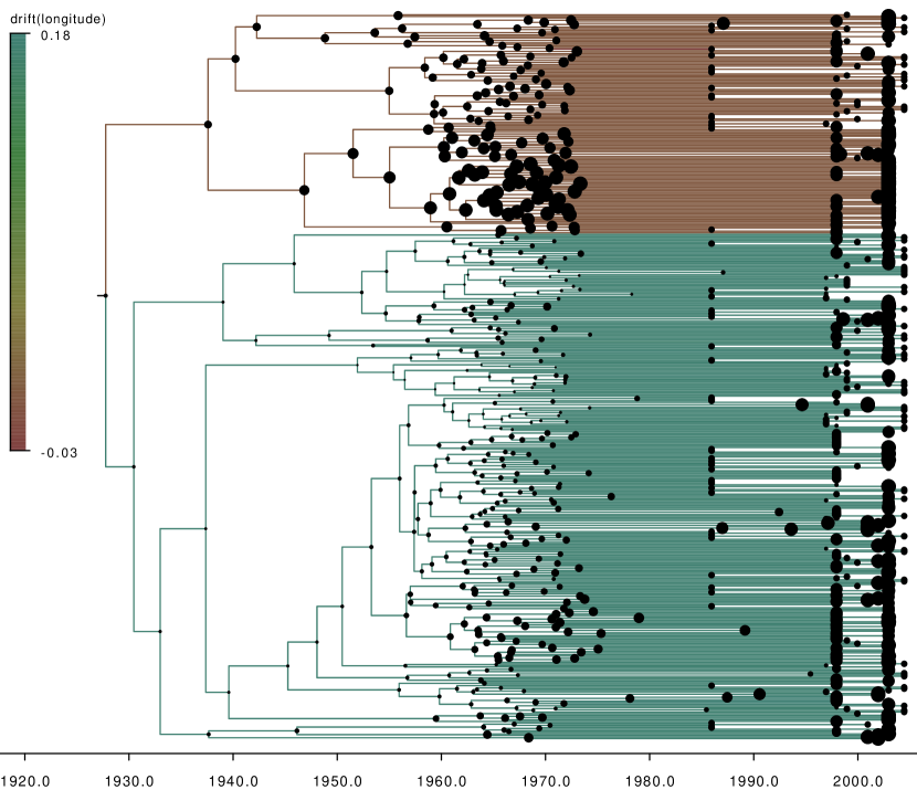
Figure 1: Maximum clade credibility tree for spread of HIV-1 in central Africa. The posterior mean longitudinal drift is depicted using a color gradient along the branches. Green indicates an eastward drift while brown signifies drift rates close to or equal to zero. Tree nodes are depicted as circles of different sizes. The size of each circle is determined by the longitude of the observed or inferred location corresponding to the node. Larger circles represent more eastward locations.

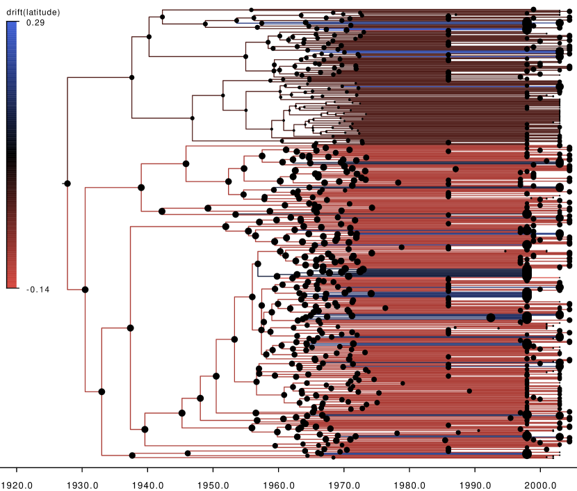
Figure 2: Maximum clade credibility tree for spread of HIV-1 in central Africa. The posterior mean latitudinal drift is depicted using a color gradient along the branches. The colors range between red and blue, with the former indicating a southward drift and the latter a northward drift. Tree nodes are depicted as circles of different sizes. The size of each circle is determined by the longitude of the observed or inferred location corresponding to the node. Larger circles represent more northward locations.

For latitudinal drift, we estimate 28.13 rate changes with BCI (27, 29). Furthermore, relaxed drift is supported over constant drift with a Bayes factor greater than 1,000. The overall posterior mean drift rate across all branches is -0.03 with BCI (-0.05, -0.01). Figure 2 depicts an annotated maximum clade credibility tree colored according to latitudinal drift rates. The color gradient ranges from red to black to blue, with red indicating a southward drift, blue a northward drift, and black a neutral drift. As in Figure 1, tree nodes are depicted as circles of varying sizes, with larger circles representing greater observed or inferred latitude coordinates. Notably, external branches with positive drift rates lead to samples from locations north of the origin (Bwamanda and Kisangani), while external branches with nonpositive drift rates lead to samples from locations with latitudes south of or similar to the origin.

Importantly, adopting a zero-mean displacement distribution when the diffusion process is more accurately described with a nontrivial mean can result in inflated displacement variance rate estimates. (Recall that the displacement variance along a branch of length $t_{i}$ is $t_{i}\textbf{P}^{-1}$, so by “displacement variance rates,” we mean the diagonal elements of the variance rate matrix $\textbf{P}^{-1}$.) By incorporating drift into the model, we are able to disentangle the drift from the variance and uncover a clearer picture of the movement. The variance rate estimates in Table 1 illustrate this point. Including a constant drift reduces the variance rate of the displacement of the longitude coordinate from 0.59 to 0.37. For the latitude, on the other hand, the variance rate decreases modestly from 0.25 to 0.23 and the BCIs of (0.23, 0.27) and (0.21, 0.25) overlap. The lack of an appreciable reduction in variance rate may be explained by the fact that the apparent northward drift to Bwamanda and Kisangani remains unaccounted for by inclusion of a constant southward drift rate. Indeed, by accommodating drift rate changes under the relaxed drift model, the variance rate of the latitudinal displacement drops to 0.13 with BCI (0.12, 0.14).

4 West Nile Virus

West Nile virus (WNV) is the most important mosquito-transmitted arbovirus now native to the U.S. Birds are the most common host, although WNV has been known to infect other animals including humans. About 70-80$\%$ of infected humans do not develop any symptoms, and most of the remaining infections result in fever and other symptoms such as headaches, body aches, joint pains, vomiting, diarrhea or rash. Fewer than 1$\%$ of infected humans will develop a serious neurologic illness such as encephalitis or meningitis. However, recovery from neurologic infection can take several months, some neurologic effects can be permanent, and about 10$\%$ of such infections lead to death. Since 1999, WNV has been responsible for more than 1,500 deaths in the United States (CDC 2013).

WNV was first detected in the United States in New York City in August 1999, and is most closely related to a highly pathogenic WNV lineage isolated in Israel in 1998 (Lanciotti et al. 1999). Surveillance records of WNV incidence show a wave of infection that spread westward and reached the west coast by 2004 (CDC 2013). Thus the spread of WNV in North America can be naturally modeled as a spatial diffusion process with a directional trend.

We analyze a data set of 104 WNV complete genome sequences sampled between 1999 and 2008 and isolated from a number of different host and vector species (Pybus et al. 2012). The sequences were sampled from a wide variety of locations in the United States and Mexico. We represent the sampling locations as bivariate traits consisting of latitude and longitude coordinates and conduct a phylogeographic analysis using our Brownian drift diffusion model. Results are presented in Table 2.

	No Drift		Constant Drift
Drift (Lat.)	-	-	-0.25	(-1.05, 0.08)
Variance (Lat.)	6.74	(4.83, 15.81)	6.38	(4.60, 14.61)
Drift (Long.)	-	-	-1.77	(-3.43, -0.27)
Variance (Long.)	23.37	(16.95, 54.04)	20.06	(14.67, 45.52)
Correlation	0.22	(0.03, 0.43)	0.18	(-0.03, 0.36)

Table 2: Spatiotemporal dynamics of West Nile virus in North America. Model comparison of Brownian diffusion with no drift and constant drift Brownian diffusion. We report posterior mean estimates along with 95$\%$ BCIs. Drift rates for latitude and longitude coordinates are reported in units of degrees per year.

We begin by analyzing the data with the constant drift model. For the longitude, the posterior mean drift rate is -1.77 degrees per year with a 95$\%$ BCI of (-3.43, -0.27). This indicates a significant westward trend in the spread of WNV, consistent with WNV incidence data. Furthermore, a Bayes factor of 18.23 lends considerable support to the constant drift model over the drift-neutral model. For the latitude, we have an estimated posterior mean drift of -0.25 degrees per year, but the 95$\%$ BCI of (-1.05, 0.08) contains zero. Moreover, the Bayes factor in favor of constant drift over no drift is 0.71. Therefore there is not much evidence of a significant North-South drift. We check for the possibility of multiple drift rates under the relaxed drift model. However, the inferred number of rate changes in the latitudinal drift is 0.63 with BCI (0, 2), and the Bayes factor in favor of relaxed drift over constant drift is 0.87. Similarly, for the longitude coordinate, we estimate 0.71 rate changes with BCI (0, 2), and Bayes factor of 1.04. Thus the data do not support relaxed drift over constant drift.

While inclusion of drift leads to smaller displacement variance rates in our analysis of HIV-1 dispersal dynamics, Table 2 shows that not to be the case for the WNV data. Even for the longitude coordinate where there is significant evidence of a nontrivial drift, there is a great deal of BCI overlap in the estimated displacement variance rate for drift-neutral and constant drift diffusion. This difference can be explained by comparing the magnitude of the displacement drift relative to the displacement standard deviation in the WNV and HIV examples. Here, we work with displacement standard deviation rather than displacement variance in order to make comparisons on the same scale. Recall that the displacement mean and variance along a branch are both proportional to the branch length. To get an estimate of the average displacement mean and standard deviation for each example, we use the mean branch length. The mean branch length is 16.9 years for the HIV data set, and 2.4 years for the WNV data set. Under constant drift, we get an average longitudinal displacement mean of 5.07 for the HIV data, and -4.25 for the WNV data. The average longitudinal displacement standard deviation without drift is 3.25 for the HIV data, and 7.49 for the WNV data. In the HIV analysis, the average displacement mean with drift is 1.61 times as much as the average displacement standard deviation without drift. In the case of the WNV, the absolute value of the average displacement mean with drift is 0.57 times as much as the average displacement standard deviation without drift. So while the displacement standard deviation in the drift-neutral HIV analysis is inflated by the hidden drift, the latent drift represents a much smaller contribution to the drift-neutral displacement standard deviation in the WNV analysis.

5 HIV-1 Resistance to Broadly Neutralizing Antibodies

It is widely believed that a successful HIV-1 vaccine will require the elicitation of neutralizing antibodies (Johnston and Fauci 2007; Barouch 2008; Walker and Burton 2008). Most neutralizing antibodies are strain-specific and therefore not so attractive for vaccine design (Weiss et al. 1985; Mascola and Montefiori 2010). It is important to identify and characterize antibody specificities that are effective against a large number of currently circulating HIV-1 variants (Burton 2002, 2004). Several broadly neutralizing monoclonal antibodies have been recently isolated, including PG9 and PG16 (Walker et al. 2009), and VRC01 (Zhou et al. 2010).

Studies comparing viruses isolated from individuals who seroconverted early in the HIV-1 epidemic to viruses from individuals who seroconverted in recent years have shown that HIV-1 has become increasingly resistant to antibody neutralization over the course of the epidemic (Bunnik et al. 2010; Euler et al. 2011; Bouvin-Pley et al. 2013). Bunnik et al. (2010) demonstrate a decreased sensitivity to polyclonal antibodies and to monoclonal antibody b12. Euler et al. (2011) extend those findings by investigating whether HIV-1 has adapted to the neutralization activity of PG9, PG16, and VRC01. Their results show that HIV-1 has become significantly more resistant to neutralization by VRC01 and also provide some support for increased resistance to neutralization by PG16.

These studies typically do not account for phylogenetic dependence among the sampled viruses. Vrancken et al. (2015) examine the data set of Euler et al. (2011) with a Brownian diffusion trait evolution model that simultaneously infers phylogenetic signal, the degree to which resemblance in traits reflects phylogenetic relatedness. They find moderate phylogenetic signal and, through ancestral trait value reconstruction, more evidence of decreased sensitivity of HIV-1 to VRC01 and PG16 neutralization at the population level.

We follow up on the analysis of Vrancken et al. (2015) by incorporating drift into the Brownian trait evolution. The data set is comprised of clonal HIV-1 variants from “historic” and “contemporary” seroconverters with an acute or early subtype B HIV-1 infection. The 14 historic seroconverters have a known seroconversion date between 1985 and 1989, and the 21 contemporary seroconverters have a seroconversion date between 2003 and 2006. The percent neutralization is determined by calculating the reduction in p24 production in the presence of the neutralizing agent compared to the p24 levels in the cultures with virus only. The trait values of interest are 50$\%$ inhibitory concentration (IC₅₀) assay values that summarize the percent neutralization by antibodies PG9, PG16 and VRC01, measured in units of $\mu$g/ml. We take the log-transform of IC₅₀ values in order to ensure that concentration values are strictly positive under the diffusion process. Higher $\log($IC${}_{50})$ values correspond to greater resistance to antibody neutralization. For viruses with $\log($IC${}_{50})$ values that fall outside the tested antibody concentration range, we integrate out the concentration over a plausible IC₅₀ interval.

First, we analyze the data with the constant drift model (see Table 3). The results are essentially consistent with the findings of Euler et al. (2011). For VRC01, we estimate a posterior mean drift of 0.15 with 95$\%$ BCI (0.06, 0.24), signaling a significant drift toward higher resistance to VRC01 neutralization. Furthermore, a Bayes factor of 32.33 lends strong support to a constant drift over no drift. There is not as much evidence of a trend for PG16. On one hand, the posterior probability that the drift rate is positive is 0.953, providing some corroboration for a decreased sensitivity to PG16 neutralization. However, we infer a mean drift rate of 0.10 with a 95$\%$ BCI of (-0.02, 0.20) that contains zero. Furthermore, the Bayes factor in favor of constant drift over no drift is just 1.32, showing little support for inclusion of a drift term. We do not detect a significant drift in the case of PG9: the posterior mean is 0.08 with 95$\%$ BCI (-0.05, 0.19) and the Bayes factor is 1.17.

To take a closer look, we fit the data to the relaxed drift model. Along with branch specific drift rates, we examine the posterior mean rates over the entire evolutionary history (see Table 3). First, we consider the results for PG9 and PG16. The posterior mean drift rates are similar to the inferred drift rates under the constant drift model, and their 95$\%$ BCIs contain 0. There is little support for any drift rate changes occurring along the phylogeny. The mean estimated number of rate changes are 0.17 and 0.2 for PG9 and PG16, respectively, and the Bayes factors in favor of relaxed drift over constant drift are 0.19 and 0.20. Hence there is not much evidence of localized directional trends that differ from the overall directional trends.

We illustrate the evolutionary pattern for resistance against VRC01 under the relaxed drift model in Figure 3. The branches of the maximum clade credibility tree are colored according to the inferred branch-specific mean drift rates, and the tree tips are labeled with subject identifications. We obtain a posterior mean estimate of 1.13 rate changes, with a posterior probability of 0.88 for exactly one rate change and probability greater than 0.99 for at least one rate change. Furthermore, the Bayes factor in favor of relaxed drift over constant drift is 359.04, providing very strong support for relaxed drift. As shown in Table 4, the displacement variance rate decreases as we move from no drift to a constant drift, and then to relaxed drift. Figure 3 shows a rate change occurring at the common ancestral node of samples from subjects P001 and P002. Apart from the two branches leading to tips P001 and P002 (which we refer to as “branch P001” and “branch P002,” respectively), the branches have essentially identical mean drift rates of about 0.15 with 95$\%$ BCI (0.09,0.21). For the blue-colored branch P001, we have an estimated drift of 2.13 with 95$\%$ BCI (0.06, 4.89), and for the red-colored branch P002 the estimated drift is -1.18 with 95$\%$ BCI (-4.46, 0.22). Both estimated drift rates are drastically different from the parent branch rate, and their BCIs are also much wider. If either subject P001 or P002 is deleted from the data set, we infer a constant, significant drift rate of 0.15 over the entire evolutionary history. Notably, we do not infer any drift rate changes after deleting either P001 or P002.

Antibody	Constant Drift		Relaxed Drift
PG9	0.08	(-0.05, 0.19)	0.07	(-0.04, 0.18)
PG16	0.10	(-0.02, 0.20)	0.11	(-0.01, 0.24)
VRC01	0.15	(0.06, 0.24)	0.15	(0.09, 0.21)

Table 3: HIV-1 resistance to broadly neutralizing antibodies. Mean drift rates under constant and relaxed drift models for $\log($IC${}_{50})$ measurements corresponding to monoclonal neutralizing antibodies PG9, PG16, and VRC01. Higher $\log($IC${}_{50})$ values represent lower sensitivity to antibody neutralization, and positive drift rates indicate a trend over time toward greater resistance. We report posterior means along with 95$\%$ BCIs.

	Displacement Variance
Antibody	No Drift		Constant Drift		Relaxed Drift
PG9	0.28	(0.18, 0.57)	0.26	(0.16, 0.53)	0.26	(0.17, 0.55)
PG16	0.26	(0.17, 0.51)	0.23	(0.15, 0.49)	0.23	(0.15, 0.51)
VRC01	0.19	(0.11, 0.43)	0.13	(0.08, 0.27)	0.06	(0.04, 0.14)

Table 4: HIV-1 resistance to broadly neutralizing antibodies. Displacement variance rate under drift-neutral, constant drift and relaxed drift models for $\log($IC${}_{50})$ measurements corresponding to monoclonal neutralizing antibodies PG9, PG16, and VRC01. We report posterior means along with 95$\%$ BCIs.

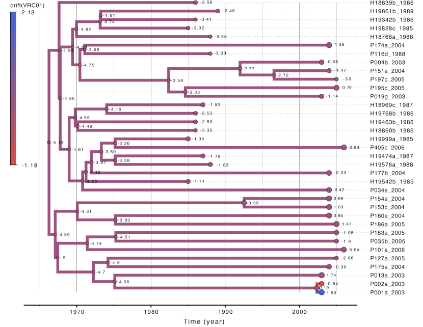
Figure 3: Maximum clade credibility tree depicting evolutionary pattern of HIV-1 resistance to neutralization by antibody VRC01. Subject identifiers corresponding to tree tips are listed to the right of the tree. The posterior mean drift is depicted using a color gradient along the branches. Positive drift rates correspond to a trend toward greater resistance to neutralization. The estimated posterior mean drift rate along the purple colored branches that make up most of the tree is 0.15. A drift rate change is inferred at the common ancestor of tips P001 and P002. The red colored branch leading to the tip P002 has an estimated posterior mean drift of -1.18, and the blue colored branch leading tip P001 has an estimated posterior mean drift of 2.13. Tree tips and internal nodes are annotated with observed and inferred $\log($IC${}_{50})$ values.

Under the relaxed drift model, situations in which both child branches have drift rates that differ from the drift rate of the parent branch must be handled with care. In any given tree in the posterior sample, one of the two branches must inherit its drift rate from the parent branch. An examination of the posterior distribution of the rate change indicator at the parent node of tips P001 and P002 reveals that branch P001 inherits the parent branch drift rate with posterior probability of about 40$\%$ and branch P002 inherits the parent rate with the other 60$\%$ probability mass. Thus the posterior drift rate estimate for each of branches P001 and P002 averages over the cases where it inherits the parent drift rate and the cases where it differs from the parent rate. While the potentially large departures from the parent drift rate still come through in the “averaged” posterior estimates, it is of interest to find out how representative they are of the true drift rates. It is conceivable that the “inherited” portion of the posterior may bias the estimate, shifting the mean and widening the BCI. In the case of branch P002, for example, the posterior mass near the parent drift rate extends the BCI into the positive axis so that it includes zero. It is also conceivable that the “inherited” part of the posterior represents a part of the distribution that would show up even without the restrictions of the relaxed drift model.

To elucidate the true nature of the drift rate change that occurs at the parent of tips P001 and P002, we conduct a follow-up analysis. We introduce a new parameterization of our drift diffusion model that posits three unique drift rates: one each corresponding to branches P001 and P002, and another for all remaining branches in the phylogenetic tree. The results, presented in Table 5, are similar to the findings from the relaxed drift model. Notably, the 95$\%$ BCIs for the drift on branches P001 and P002 still contain the range of credible values for the parent drift rate. There are also some key differences between the two analyses. The distributions for the drift on branches P001 and P002 are bell-shaped rather than bimodal, and the 95$\%$ BCIs are wider than under the relaxed drift model. Unlike the relaxed drift model estimate, the 95$\%$ BCI for the drift on branch P001 contains 0. However, it has a 0.95 posterior probability of being positive, so there is still some support that the drift on branch P001 is statistically significant.

An examination of the maximum clade credibility tree in Figure 3, annotated with observed $\log($IC${}_{50})$ values and inferred ancestral trait realizations, clarifies why we infer a drift rate change. Consider node triples consisting of two nodes and their common parent node. The triple of tips P001, P002 and their common ancestor features a relatively large difference in trait values at the child nodes as well as relatively short branch lengths connecting nodes P001 and P002 to their parent. While there are other triples with child nodes possessing a comparable difference in $\log($IC${}_{50})$ values, they have much longer branches leading from the parent node to the children. Similarly, while other triples feature relatively short branches connecting the parent to the children, the trait values at the child nodes do not differ as much. The unique combination of short branches coupled with a large difference between $\log($IC${}_{50})$ values at the child nodes explains why the drift rate present on most of the tree may be incompatible with the triple of P001, P002 and their parent.

	Relaxed Drift			Fixed-Changes
Branch	Mean	95$\%$ BCI	P(Drift $>$ 0)	Mean	95$\%$ BCI	P(Drift $>$ 0)
P001	2.13	(0.06, 4.89)	$>$ 0.99	2.27	(-0.36, 5.10)	0.95
P002	-1.18	(-4.46, 0.22)	0.60	-1.81	(-4.61, 1.03)	0.10
Other	0.15	(0.09, 0.21)	$>$ 0.99	0.14	(0.08, 0.20)	$>$ 0.99

Table 5: Rate changes in HIV-1 drift toward resistance to antibody VRC01. We report posterior means, 95$\%$ BCIs, and posterior probabilities that the drift $>0$.

Although there is strong evidence of a drift rate change at the ancestral node of samples P001 and P002, the wide BCIs for the branch P001 and branch P002 drift rate estimates suggest that they are poorly informed by the data. The type of drift rate change that occurs at the ancestral node of tips P001 and P002 also remains unclear. Subjects P001 and P002 are a transmission couple and it appears that one person mounted a very different antibody response than the other to a highly similar virus. Further research may clarify the situation. Nevertheless, we infer a clear, significant drift towards increased resistance to neutralization by VRC01, and it is robust to deletion of either subject P001 or P002. At the population level, the phylogenetic structure of HIV is “starlike,” featuring multiple co-circulating lineages, the dynamics of which generally reflects neutral epidemiological processes (Grenfell et al. 2004). It is therefore notable to find evidence of population level evolution towards increased resistance.

6 Discussion

Standard Brownian diffusion is a popular and, in many ways, natural starting point for modeling continuous trait evolution in a phylogenetic context. On the other hand, it is very restrictive and may not adequately describe the dynamics of the underlying evolutionary process. Development of non-Brownian models, such as mean-reverting Ornstein-Uhlenbeck processes, represents a promising avenue. However, substantial gains can also be made through building upon standard Brownian diffusion approaches. For example, the displacement along a branch is typically assumed to have variance equal to the product of the branch length and a diffusion variance rate matrix $\textbf{P}^{-1}$, where $\textbf{P}^{-1}$ does not vary along the phylogenetic tree. Lemey et al. (2010) demonstrate improvements by relaxing this homogeneity assumption via branch-specific diffusion rate scalars that yield a mixture of Brownian processes. Here, we show that progress towards a more realistic trait diffusion can be made by relaxing the assumption of a zero-mean displacement. Furthermore, the drift diffusion approach we consider is very general. Notably, the Ornstein-Uhlenbeck process is nested within the drift diffusion process defined by

$$\textbf{Y}_{i}|\textbf{Y}_{pa(i)}\sim N\left(\bm{\beta}_{1}(t_{i})\textbf{Y}_{pa(i)}+\bm{\beta}_{2}(t_{i})\bm{\mu}_{i},\bm{\Sigma}(t_{i})\right).$$ (45)

Consider the special case where $\bm{\mu}_{i}=\bm{\mu}$ for every branch, and

$$\bm{\beta}_{1}(t_{i})=e^{-\alpha t_{i}},\leavevmode\nobreak\ \leavevmode\nobreak\ \bm{\beta}_{2}(t_{i})=1-e^{-\alpha t_{i}},\leavevmode\nobreak\ \leavevmode\nobreak\ \text{and}\leavevmode\nobreak\ \leavevmode\nobreak\ \bm{\Sigma}(t_{i})=\frac{\sigma^{2}}{2\alpha}\left[1-e^{-2\alpha t_{i}}\right].$$ (46)

This is equivalent to an Ornstein-Uhlenbeck process on the phylogenetic tree defined by the stochastic differential equation

$$d\textbf{Y}_{t}=\alpha(\bm{\mu}-\textbf{Y}_{t})dt+\sigma d\textbf{W}_{t},$$ (47)

where $\textbf{W}_{t}$ is a standard Brownian diffusion process. Here, $\bm{\mu}$ can be thought of as an optimal trait value, $\alpha$ represents the strength of selection towards $\bm{\mu}$, and $\sigma^{2}$ is the variance of the Brownian diffusion component. Such generality enables formal testing between a wide class of different Gaussian process models.

We introduce a flexible new Bayesian framework for phylogenetic trait evolution, modeling the evolutionary process as Brownian diffusion with a nontrivial drift. By allowing an estimable mean vector in the displacement distribution, we can account for and quantify a directional trend. However, imposing a constant drift rate can make for an unrealistic approximation of the underlying process. We overcome this limitation through the relaxed drift model. The relaxed drift model permits drift rate variation along a phylogenetic tree while maintaining model identifiability. Drift rates are generally passed on from parent branches to child branches, and variation is achieved by allowing at most one branch of any given pair of child branches to assume a different drift rate from their common parent branch.

The utility of incorporating drift into the diffusion is corroborated by our analyses of three viral examples. We apply our methodology to both geographic traits in a phylogeographic setting as well as phenotypic traits. Our phylogeographic analysis of the spread of HIV-1 in central Africa confirms the findings obtained by discrete phylogeographic inference (Faria et al. 2014). Drift diffusion models fit the data better than drift-neutral Brownian diffusion, and we uncover directional trends in the dispersal of the virus from its origin to sampling locations. We also see that drift rate variation characterizes real spatiotemporal diffusion processes. The absence of drift in the diffusion model can lead to conflation of the latent drift with other parameters, particularly the displacement variance. Our analysis of the spread of HIV-1 illustrates how inferred displacement variance rates can decrease with appropriate drift rate modeling, revealing a clearer, more detailed picture of dispersal dynamics.

While it is tempting to assume drift rate variation and seek out the additional insight it may provide, the data may not support multiple drift rates. This may be the case even when there is a significant constant drift, as we see in our analysis of the West Nile virus. Parameterizing the model to allow the maximal number of unique drift rates can result in numerous small rate changes that are a consequence of the modeling choice and are not necessarily driven by the data. Our relaxed drift framework overcomes this issue by inferring the locations and types of rate changes directly from the data as opposed to making a priori assumptions about the number of unique drift rates and their appropriate assignments. Bayesian stochastic search variable selection enables efficient exploration of all possible drift rate configurations.

Although our focus has been on drift, a major strength of our approach is its implementation in the larger Bayesian phylogenetic framework of BEAST. Through BEAST, we have access to a plethora of different models for molecular character substitution, demographic history and molecular clocks. Bayesian inference provides a natural framework for controlling for different sources of uncertainty in evolutionary models, including the phylogenetic tree and trait and sequence evolution parameters, and testing evolutionary hypotheses.

The gains from introducing drift into our real data examples are encouraging, and there is a need for continued development of more realistic trait evolutionary models. We anticipate that our drift diffusion approach will be useful in other scenarios not examined here, including antigenic drift in influenza. Antigenic drift is the process by which influenza viruses evolve to evade the immune system, and an understanding of its dynamics is essential to public health efforts. Bedford et al. (2014) have recently developed an integrated approach to mapping antigenic phenotypes that combines it with genetic information. It may be fruitful to model the diffusion of the antigenic phenotype in their framework with a relaxed drift.

While the relaxed drift model has proven to be flexible and useful, its identifiability restrictions may render it inappropriate for some evolutionary scenarios. For example, once a drift rate appears anywhere in the phylogenetic tree, the restrictions mandate that it must be passed on and “survive” until it reaches an external branch. Lack of support for the survival of a specific drift rate may not preclude its inclusion under relaxed drift. In the analysis of HIV-1 resistance to neutralization, for example, the parent branch of branches P001 and P002 must pass on its drift rate to one of the two child branches in each tree in the posterior sample. Yet, the branch which is forced to inherit the parent drift rate alternates between P001 and P002 in the posterior sample, resulting in posterior drift distributions for both branches that differ from that of their parent drift. However, this unnatural mechanism of deflecting an unsupported drift rate may contribute to misleading drift rate estimates. It would be preferable to sidestep such problems by developing alternative models that accommodate drift rate variation while retaining identifiability.

Appendix

Appendix A Identifiability

To ensure that our results are meaningful, it is important to understand the conditions under which our model is identifiable. For convenience, and without loss of generality, we assume here that traits are one-dimensional. Following the development in section 2.1, the observed traits $\textbf{Y}=(\textbf{Y}_{1},\dots,\textbf{Y}_{N})^{t}$ at the tips of the phylogeny $\tau$ are multivariate-normal distributed:

$$P\left(\textbf{Y}|\textbf{Y}_{2N-1},\textbf{P},\textbf{V}_{\tau},\bm{\mu}_{\tau}\right)=\mbox{MVN}\left(\textbf{Y};\textbf{Y}_{\text{root}}+\textbf{T}\bm{\mu}_{\tau},\textbf{P}^{-1}\otimes\textbf{V}_{\tau}\right).$$ (48)

Here, $\textbf{Y}_{\text{root}}$ is an $N\times 1$ vector with the root trait $\textbf{Y}_{2N-1}$ repeated $N$ times. The vector $\bm{\mu}_{\tau}=(\bm{\mu}_{1},\dots,\bm{\mu}_{2N-2})^{t}$ consists of branch-specific drift rates $\bm{\mu}_{i}$. The $N\times N$ variance matrix $\textbf{V}_{\tau}$ is a deterministic function of $\tau$ and represents the contribution of the phylogenetic tree to the covariance structure. Its diagonal entries $V_{ii}$ are equal to the distance in time between the tip $\mathcal{V}_{i}$ and the root node $\mathcal{V}_{2N-1}$, and off-diagonal entries $V_{ij}$ correspond to the distance in time between the root node $\mathcal{V}_{2N-1}$ and the most recent common ancestor of tips $\mathcal{V}_{i}$ and $\mathcal{V}_{j}$. Finally, the $N\times(2N-2)$ matrix T is defined as follows: $T_{ij}=t_{j}$, the length of branch $j$, if branch $j$ is part of the path from the external node $i$ to the root, and $T_{ij}=0$ otherwise. In other words, the $i$th row of T specifies the path of branches in $\tau$ connecting external node $i$ to the root.

Let $\textbf{V}(\bm{\mu}_{\tau})$ denote the vector space of permissible values of $\bm{\mu}_{\tau}$ for our model. With respect to the drift, the model is identifiable if the equality

$$P\left(\textbf{Y}|\textbf{Y}_{2N-1},\textbf{P},\textbf{V}_{\tau},\bm{\mu}_{\tau}\right)=P\left(\textbf{Y}|\textbf{Y}_{2N-1},\textbf{P},\textbf{V}_{\tau},\bm{\mu}_{\tau}^{*}\right)$$ (49)

implies that $\bm{\mu}_{\tau}=\bm{\mu}_{\tau}^{*}$. Because the drift appears only in the mean of the distribution, we have an identifiability problem if the same mean $\mathrm{E}(\textbf{Y})$ can be realized from different values of $\bm{\mu}_{\tau}$. In other words, if there exist $\bm{\mu}_{\tau}\neq\bm{\mu}_{\tau}^{*}$ such that $\textbf{T}\bm{\mu}_{\tau}=\textbf{T}\bm{\mu}_{\tau}^{*}$. This can happen if and only if the linear transformation T has a nontrivial kernel. We know that

$$\mbox{dim}\textbf{V}(\bm{\mu}_{\tau})=\mbox{dim ker}(\textbf{T})+\mbox{dim range}(\textbf{T}),$$ (50)

and we also know that for any phylogeny $\tau$, T is of full rank because its rows are linearly independent. It follows that for the kernel of T to be trivial, we must have

$$\mbox{dim}\textbf{V}(\bm{\mu}_{\tau})\leq N.$$ (51)

If we allow a unique drift rate on each branch of $\tau$, we have $\textbf{V}(\bm{\mu}_{\tau})=\mathbb{R}^{2\mathbb{N}-2}$. Therefore we must take a different approach.

It is illuminating to look at identifiability from the perspective of linear equations. For a given $\bm{\mu}_{\tau}$, T maps $\bm{\mu}_{\tau}$ to an $N\times 1$ vector $\bm{\gamma}$:

$$\textbf{T}\bm{\mu}_{\tau}=\bm{\gamma}.$$ (52)

Identifiability is then equivalent to the system (52) of $N$ linear equations having a unique solution.

To achieve identifiability, we introduce the relaxed drift model. Starting with a drift rate on the unobserved branch leading to the root node and moving down the tree toward the external nodes, every time a branch splits into two branches, one of two things happens. Either both of the child branches inherit the drift rate of the parent branch, or exactly one of the child branches inherits the drift rate from the parent branch while the other gets a new drift rate. Both child branches taking on different drift rates than the parent branch is not permitted. To avoid confusion, we continue to denote the $2N-2$ branch-specific drift rates as $\bm{\mu}_{1},\dots,\bm{\mu}_{2N-2}$, with the understanding that they are not all unique. We let $\bm{\mu}^{*}_{1},\dots,\bm{\mu}^{*}_{K}$ denote the unique drift rates, where $K\leq N$.
Definition: We say that a row $\textbf{T}_{i}=(T_{i1},T_{i2},\dots,T_{i,2N-2})$ in T is $\bm{\mu}^{*}_{k}-\textit{dominated}$ if its associated path from the root of $\tau$ to a tip ends with a branch with drift rate $\bm{\mu}^{*}_{k}$. We also refer to the sum $\textbf{T}_{i}\bm{\mu}_{\tau}=\sum_{j=1}^{2N-2}T_{ij}\bm{\mu}_{j}$ and the path associated with $\textbf{T}_{i}$ as $\bm{\mu}^{*}_{k}-\textit{dominated}$.
Note that each unique drift rate dominates at least one path.
Definition: An initial branch of the rate $\bm{\mu}^{*}_{k}$ is a branch whose parent branch has a different drift rate. The unobserved branch leading to the root node is also defined to be an initial branch.
Observe that every branch with drift $\bm{\mu}^{*}_{k}$ is an initial branch of $\bm{\mu}^{*}_{k}$ or a descendant of an initial branch of $\bm{\mu}^{*}_{k}$. A drift rate may have more than one initial branch. In order to quantify how deep into the tree $\tau$ a drift rate extends (starting from the tips and going toward the root), we make the following definition.
Definition: By a descendant path of a branch $b$, we mean a series of connected branches, starting with a child branch of $b$ and ending with a branch leading to a tip. The depth of a branch $b$ is equal to the maximal number of branches in descendant paths of $b$. The depth of a drift rate $\bm{\mu}^{*}_{k}$ is equal to the maximal depth of its initial branches.
For example, if $\bm{\mu}^{*}_{k}$ has one initial branch leading to a tip, then $\bm{\mu}^{*}_{k}$ has depth 0. If the number of unknowns $K$ is less than the number of equations $N$ in the system $\textbf{T}\bm{\mu}_{\tau}=\bm{\gamma}$, a unique solution can be established by working with a reduced system. We form the reduced system by choosing $K$ of the $N$ rows in T, say $\textbf{T}_{i_{1}},\dots,\textbf{T}_{i_{K}}$, such that each is dominated by a different drift rate. If a drift rate dominates more than one path, we choose a path containing a maximal depth initial branch of the rate for the reduced system.
Claim: The relaxed drift model is identifiable.
Proof: The reduced linear system

$$\sum_{j=1}^{2N-2}T_{i_{1}j}\bm{\mu}_{j} = \bm{\gamma}_{i_{1}}$$ (53)

$$\sum_{j=1}^{2N-2}T_{i_{2}j}\bm{\mu}_{j} = \bm{\gamma}_{i_{2}}$$ (54)

$$\dots$$ (55)

$$\sum_{j=1}^{2N-2}T_{i_{K}j}\bm{\mu}_{j} = \bm{\gamma}_{i_{K}},$$ (56)

consists of $K$ equations and $K$ variables. Therefore to show that the solution is unique, it suffices to show that the linear system is independent. To establish independence, it suffices to show that if

$$a_{1}\sum_{j=1}^{2N-2}T_{i_{1}j}\bm{\mu}_{j}+a_{2}\sum_{j=1}^{2N-2}T_{i_{2}j}\bm{\mu}_{j}\dots+a_{N}\sum_{j=1}^{2N-2}T_{i_{K}j}\bm{\mu}_{j}=0,$$ (57)

for some constants $a_{1},\dots,a_{K}$, then we must have

$$a_{1}=a_{2}=\dots=a_{K}=0.$$ (58)

Suppose (57) holds. The idea behind the proof is as follows: we consider all drift rates of depth 0, conclude that each sum in (57) dominated by a drift rate of depth 0 must have its corresponding coefficient $a_{i}=0$, then consider all drift rates of depth 1, conclude that each sum in (57) dominated by a drift rate of depth 1 must have corresponding coefficient $a_{i}=0$, and so on until we have gone through all possible depth values of drift rates in $\tau$.

Suppose $\bm{\mu}^{*}_{k}$ has depth 0. Then $\bm{\mu}^{*}_{k}$ only appears in the single $\bm{\mu}^{*}_{k}-$dominated sum and cannot be canceled out by a linear combination of the other sums. This forces the coefficient $a_{i}$ of the $\bm{\mu}^{*}_{k}-$dominated sum in (57) to be equal to zero. Having shown that any sum dominated by a drift rate of depth 0 must have a zero coefficient in (57), we can move on to the case of depth 1. Rather than handle the case of depth 1 separately, we present a general argument.

Suppose the coefficients of all sums in (57) that are dominated by drift rates of depth less than $m$ have been shown to be zero. Consider drift rates of depth $m$. If $\bm{\mu}^{*}_{k}$ has depth $m$, then it appears in the $\bm{\mu}^{*}_{k}-$dominated path, and it may appear in paths dominated by other rates. Suppose $\bm{\mu}^{*}_{k}$ appears in a path $P_{i}$ dominated by a different rate, say $\bm{\mu}^{*}_{i}$. By construction of the reduced system, $P_{i}$ contains an initial branch $\textbf{b}_{i}$ of $\bm{\mu}^{*}_{i}$ of maximal depth. This means the depth of $\textbf{b}_{i}$ is equal to the depth of $\bm{\mu}^{*}_{i}$. Because $\textbf{b}_{i}$ is a descendant of a branch with rate $\bm{\mu}^{*}_{k}$, the depth of $\bm{\mu}^{*}_{i}$ must be less than the depth of $\bm{\mu}^{*}_{k}$. But sums dominated by rates of depth less than $m$ have already been shown to have zero coefficients in (57). Thus the sum associated with $P_{i}$ has coefficient zero. Because $\bm{\mu}^{*}_{k}$ appears in only one sum which is not already known to have a zero coefficient, the $\bm{\mu}^{*}_{k}-$dominated sum, it follows that in order for (57) to hold, the $\bm{\mu}^{*}_{k}-$dominated sum must also have a zero coefficient. Therefore sums dominated by drift rates of depth $m$ must have zero coefficients in (57).

Invoking this argument until we have gone through all possible values of drift rate depth, it follows that $a_{1}=a_{2}=\dots=a_{K}=0$. $\blacksquare$

References

- Allicock et al. (2012) Allicock, O. M., P. Lemey, A. J. Tatem, O. G. Pybus, S. N. Bennett, B. A. Mueller, M. A. Suchard, J. E. Foster, A. Rambaut, and C. V. Carrington. 2012. Phylogeography and population dynamics of dengue viruses in the americas. Molecular Biology and Evolution 29:1533–1543.
- Baele and Lemey (2013) Baele, G. and P. Lemey. 2013. Bayesian evolutionary model testing in the phylogenomics era: matching model complexity with computational efficiency. Bioinformatics 29:1970–1979.
- Baele et al. (2012) Baele, G., P. Lemey, T. Bedford, A. Rambaut, M. A. Suchard, and A. V. Alekseyenko. 2012. Improving the accuracy of demographic and molecular clock model comparison while accommodating phylogenetic uncertainty. Molecular Biology and Evolution 29:2157–2167.
- Baele et al. (2013) Baele, G., W. L. S. Li, A. J. Drummond, M. A. Suchard, and P. Lemey. 2013. Accurate model selection of relaxed molecular clocks in Bayesian phylogenetics. Molecular Biology and Evolution 30:239–243.
- Barouch (2008) Barouch, D. 2008. Challenges in the development of an HIV-1 vaccine. Nature 455:613–619.
- Bartoszek et al. (2012) Bartoszek, K., J. Pienaar, P. Mostad, S. Andersson, and T. Hansen. 2012. A phylogenetic comparative method for studying multivariate adaptation. Journal of Theoretical Biology 314:204–215.
- Bedford et al. (2014) Bedford, T., M. Suchard, P. Lemey, G. Dudas, V. Gregory, A. Hay, J. McCauley, C. Russell, D. Smith, and A. Rambaut. 2014. Integrating influenza antigenic dynamics with molecular evolution. Elife 3:e01914.
- Bennett et al. (2010) Bennett, S., A. Drummond, D. Kapan, M. Suchard, J. Munoz-Jordan, O. Pybus, E. Holmes, and D. Gubler. 2010. Epidemic dynamics revealed in dengue evolution. Molecular Biology and Evolution 27:811–818.
- Biek et al. (2007) Biek, R., J. Henderson, L. Waller, C. Rupprecht, and L. Real. 2007. A high-resolution genetic signature of demographic and spatial expansion in epizootic rabies virus. PNAS 104:7993–7998.
- Bikandou et al. (2004) Bikandou, B., M. Ndoundou-Nkodia, F. Niama, M. Ekwalanga, O. Obengui, R. Taty-Taty, H. Parra, and S. Saragosti. 2004. Genetic subtyping of gag and env regions of HIV type 1 isolates in the Republic of Congo. AIDS Research and Human Retroviruses 20.
- Bikandou et al. (2000) Bikandou, B., J. Takehisa, I. Mboudjeka, E. Ido, T. Kuwata, Y. Miyazaki, H. Moriyama, Y. Harada, Y. Taniguchi, H. Ichimura, M. Ikeda, P. Ndolo, M. Nzoukoudi, R. M’Vouenze, M. M’Pandi, H. Parra, P. M’Pele, and M. Hayami. 2000. Genetic subtypes of HIV type 1 in Republic of Congo. AIDS Research and Human Retroviruses 16:613–619.
- Bloomquist et al. (2010) Bloomquist, E. W., P. Lemey, and M. A. Suchard. 2010. Three roads diverged? routes to phylogeographic inference. Trends in Ecology & Evolution 25:626–632.
- Bouvin-Pley et al. (2013) Bouvin-Pley, M., M. Morgand, A. Moreau, P. Jestin, C. Simonnet, L. Tran, C. Goujard, L. Meyer, F. Barin, and M. Braiband. 2013. Evidence for a continuous drift of the HIV-1 species towards higher resistance to neutralizing antibodies over the course of the epidemic. PLoS Pathogens 9:e1003477.
- Brown (1828) Brown, R. 1828. A brief account of microscopial observations made in the months of June, July and August, 1827, on the particles contained in the pollen of plants; and on the general existence of active molecules in organic and inorganic bodies. Philosophical Magazine 4:161–173.
- Bunnik et al. (2010) Bunnik, E., Z. Euler, M. Welkers, B. Boeser-Nunnink, M. Grijsen, J. Prins, and H. Schuitemaker. 2010. Adaptation of HIV-1 envelope gp120 to humoral immunity at a population level. Nature Medicine 16:995–997.
- Burton (2002) Burton, D. 2002. Antibodies, viruses and vaccines. Nature Reviews Immunology 2:706–713.
- Burton (2004) Burton, D. 2004. HIV vaccine design and the neutralizing antibody problem. Nature Immunology 5:233–236.
- Butler and King (2004) Butler, M. and A. King. 2004. Phylogenetic comparative analysis: a modeling approach for adaptive evolution. American Naturalist 164.
- CDC (2013) CDC. 2013. Centers for disease control and prevention, West Nile Virus. http://www.cdc.gov/westnile.
- Chipman et al. (2001) Chipman, H., E. George, and R. McCulloch. 2001. The practical implementation of Bayesian model selection. IMS Lecture Notes - Monograph Series 38:67–134.
- Cybis et al. (2015) Cybis, G. B., J. S. Sinsheimer, T. Bedford, A. E. Mather, P. Lemey, and M. A. Suchard. 2015. Assessing phenotypic correlations through the multivariate phylogenetic latent liability model. Annals of Applied Statistics 9:969–991.
- Drummond et al. (2006) Drummond, A., S. Ho, M. Phillips, and A. Rambaut. 2006. Relaxed phylogenetics and dating with confidence. PLoS Biology 4:e88.
- Drummond and Suchard (2010) Drummond, A. and M. Suchard. 2010. Bayesian random local clocks, or one rate to rule them all. BMC Biology 8.
- Drummond et al. (2012) Drummond, A. J., M. A. Suchard, D. Xie, and A. Rambaut. 2012. Bayesian phylogenetics with BEAUti and the BEAST 1.7. Molecular Biology and Evolution 29:1969–1973.
- Euler et al. (2011) Euler, Z., E. Bunnik, J. Burger, B. Boeser-Nunnink, M. Grijsen, J. Prins, and H. Schuitemaker. 2011. Activity of broadly neutralizing antibodies, including PG9, PG16, and VRC01, against recently transmitted subtype B HIV-1 variants from early and late in the epidemic. Journal of Virology 85:7236–7245.
- Faria et al. (2014) Faria, N., A. Rambaut, M. Suchard, G. Baele, T. Bedford, M. Ward, A. Tatem, J. Sousa, N. Arinaminpathy, J. Pepin, D. Posada, M. Peeters, O. Pybus, and P. Lemey. 2014. The early spead and epidemic ignition of HIV-1 in human populations. Science 346:56–61.
- Felsenstein (1973) Felsenstein, J. 1973. Maximum-likelihood estimation of evolutionary trees from continuous characters. American Journal of Human Genetics 25:471–492.
- Felsenstein (1981) Felsenstein, J. 1981. Evolutionary trees from DNA sequences: a maximum likelihood approach. Journal of Molecular Evolution 13:93–104.
- Felsenstein (1985) Felsenstein, J. 1985. Phylogenies and the comparative method. The American Naturalist 125:1–15.
- Freckleton et al. (2002) Freckleton, R., P. Harvey, and M. Pagel. 2002. Phylogenetic analysis and comparative data: A test and review of evidence. The American Naturalist 160:712–726.
- George and McCulloch (1993) George, E. and R. McCulloch. 1993. Variable selection via Gibbs sampling. Journal of American Statistical Association 88:881–889.
- Gill et al. (2013) Gill, M., P. Lemey, N. Faria, A. Rambaut, B. Shapiro, and M. Suchard. 2013. Improving Bayesian population dynamics inference: a coalescent-based model for multiple loci. Molecular Biology and Evolution 30:713–724.
- Grenfell et al. (2004) Grenfell, B., O. Pybus, J. Gog, J. Wood, J. Daly, J. Mumford, and E. Holmes. 2004. Unifying the epidemiological and evolutionary dynamics of pathogens. Science 303:327–332.
- Hansen (1997) Hansen, T. 1997. Stabilizing selection and the comparative analysis of adaptation. Evolution 52:1341–1351.
- Harvey and Pagel (1991) Harvey, P. and M. Pagel. 1991. The comparative method in evolutionary biology. Oxford University Press.
- Hasegawa et al. (1985) Hasegawa, M., H. Kishino, and T. Yano. 1985. Dating the human-ape splitting by a molecular clock of mitochondrial DNA. Journal of Molecular Evolution 22:160–174.
- Hastings (1970) Hastings, W. 1970. Monte Carlo sampling methods using Markov chains and their applications. Biometrika 57:97–109.
- Huelsenbeck and Rannala (2003) Huelsenbeck, J. and B. Rannala. 2003. Detecting correlation between characters in a comparative analysis with uncertain phylogeny. Evolution 57:1237–1247.
- Jeffreys (1935) Jeffreys, H. 1935. Some tests of significance, treated by the theory of probability. Mathematical Proceedings of the Cambridge Philosophical Society 31:203–222.
- Jeffreys (1961) Jeffreys, H. 1961. Theory of Probability. Oxford University Press.
- Johnston and Fauci (2007) Johnston, M. and A. Fauci. 2007. An HIV vaccine: evolving concepts. New England Journal of Medicine 356:2073–2080.
- Kalish et al. (2004) Kalish, M., K. Robbins, D. Pieniazek, A. Schaefer, N. Nzilambi, T. Quinn, M. S. Louis, A. Youngpairoj, J.Phillips, H. Jaffe, and T. Folks. 2004. Recombinant viruses and early global HIV-1 epidemic. Emerging Infectious Diseases 10:1227–1234.
- Kass and Raftery (1995) Kass, R. and A. Raftery. 1995. Bayes factors. Journal of the American Statistical Association 90:773–795.
- Kimura (1980) Kimura, M. 1980. A simple method for estimating evolutionary rates of base substitutions through comparative studies of nucleotide sequences. Journal of Molecular Evolution 16:111–120.
- Kita et al. (2004) Kita, K., N. Ndembi, M. Ekwalanga, E. Ido, R. Kazadi, B. Bikandou, J. Takehisa, T. Takemura, S. Kageyama, J. Tanaka, H. Parra, M. Hayami, and H. Ichimura. 2004. Genetic diversity of HIV type 1 in Likasi, southeast of the Democratic Republic of Congo. AIDS Research and Human Retroviruses 20:1352–1357.
- Kuo and Mallick (1998) Kuo, L. and B. Mallick. 1998. Variable selection for regression models. Sankhya B 60:65–81.
- Lanciotti et al. (1999) Lanciotti, R., J. Roehrig, V. Deubel, J. Smith, M. Parker, K. Steele, B. Crise, K. Volpe, M. Crabtree, J. Scherret, R. Hall, J. MacKenzie, C. Cropp, B. Panigrahy, E. Ostlund, B. Schmitt, M. Malkinson, C. Banet, J. Weissman, N. Komar, H. Savage, W. Stone, T. McNamara, and D. Gubler. 1999. Origin of the West Nile virus responsible for an outbreak of encephalitis in the northeastern United States. Science 286:2333–2337.
- Lartillot and Poujol (2011) Lartillot, N. and R. Poujol. 2011. A phylogenetic model for investigating correlated evolution of subsitution rates and continuous phenotypic characters. Molecular Biology and Evolution 28:729–744.
- Lemey et al. (2009a) Lemey, P., A. Rambaut, A. Drummond, and M. Suchard. 2009a. Bayesian phylogeography finds its roots. PLoS Computational Biology 5:e1000520.
- Lemey et al. (2010) Lemey, P., A. Rambaut, J. Welch, and M. Suchard. 2010. Phylogeography takes a relaxed random walk in continuous space and time. Molecular Biology and Evolution 27:1877–1885.
- Lemey et al. (2009b) Lemey, P., M. Suchard, and A. Rambaut. 2009b. Reconstructing the initial global spread of a human influenza pandemic: a Bayesian spatial-temporal model for the global spread of H1N1. PLoS Currents RRN1031.
- Mascola and Montefiori (2010) Mascola, J. and D. Montefiori. 2010. The role of antibodies in HIV vaccines. Annual Review of Immunology 28:413–444.
- Mello et al. (2013) Mello, F., O. Araujo, B. Lago, A. Motta-Castro, M. Moraes, S. Gomes, G. Bello, and N. Araujo. 2013. Phylogeography and evolutionary history of hepatitis B virus genotype F in Brazil. Virology Journal 10:236.
- Metropolis et al. (1953) Metropolis, N., A. Rosenbluth, M. Rosenbluth, A. Teller, and E. Teller. 1953. Equation of state calculation by fast computing machines. Journal of Chemical Physics 21:1087–1092.
- Minin et al. (2008) Minin, V., E. Bloomquist, and M. Suchard. 2008. Smooth skyride through a rough skyline: Bayesian coalescent based inference of population dynamics. Mol Biol Evol 25:1459–1471.
- Niama et al. (2006) Niama, F., C. Toure-Kane, N. Vidal, P. Obengui, B. Bikandou, M. Ndoundou-Nkodia, C. Montavon, H. Diop-Ndiaye, J. Mombouli, E. Mokondzimobe, A. Diallo, E. Delaporte, H. Parra, M. Peeters, and S. Mboup. 2006. HIV-1 subtypes and recombinants in the Republic of Congo. Infection, Genetics and Evolution 6:337–343.
- Pagel (1999) Pagel, M. 1999. The maximum likelihood approach to reconstructing ancestral character states of discrete characters on phylogenies. Systematic Biology 48:612–622.
- Pybus et al. (2012) Pybus, O., M. Suchard, P. Lemey, F. Bernardin, A. Rambaut, F. Crawford, R. Gray, N. Arinaminpathy, S. Stramer, M. Busch, and E. Delwart. 2012. Unifying the spatial epidemiology and molecular evolution of emerging epidemics. PNAS 109:15066–71.
- Rambaut et al. (2008) Rambaut, A., O. Pybus, M. Nelson, C. Viboud, J. Taubenberger, and E. Holmes. 2008. The genomic and epidemiological dynamics of human influenza A virus. Nature 453:615–619.
- Seetahal et al. (2013) Seetahal, J., A. Velasco-Billa, O. Allicock, A. Adesiyun, J. Bissessar, K. Amour, A. Phillip-Hosein, D. Marston, L. McElhinney, M. Shi, C. Wharwood, A. Fooks, and C. Carrington. 2013. Evolutionary history and phylogeography of rabies viruses associated with outbreaks in Trinidad. PLoS Neglected Tropical Diseases 7:e2365.
- Sinsheimer et al. (1996) Sinsheimer, J., J. Lake, and R. Little. 1996. Bayesian hypothesis testing of four-taxon topologies using molecular sequence data. Biometrics 52:193–210.
- Smith et al. (2009) Smith, G., D. Vijaykrishna, J. Bahl, S. Lycett, M. Worobey, O. Pybus, S. Ma, C. Cheung, J. Raghwani, S. Bhatt, J. Peiris, Y. Guan, and A. Rambaut. 2009. Origins and evolutionary genomics of the 2009 swine-origin H1N1 influenza A epidemic. Nature 459:1122–1125.
- Suchard et al. (2001) Suchard, M., R. Weiss, and J. Sinsheimer. 2001. Bayesian selection of continuous-time Markov chain evolutionary models. Molecular Biology and Evolution 18:1001–1013.
- Suchard et al. (2005) Suchard, M., R. Weiss, and J. Sinsheimer. 2005. Models for estimating Bayes factors with applications to phylogeny and tests of monophyly. Biometrics 61:665–673.
- Vidal et al. (2005) Vidal, N., C. Mulanga, S. Bazepeo, J. Mwamba, J. Tshimpaka, M. Kashi, N. Mama, C. Laurent, F. Lepira, E. Delaporte, and M. Peeters. 2005. Distribution of HIV-1 variants in the Democratic Republic of Congo suggests increase of subtype C in Kinshasa between 1997 and 2002. Journal of Acquired Immune Deficiency Syndromes 40:456–462.
- Vidal et al. (2000) Vidal, N., M. Peeters, C. Mulanga-Kabeya, N. Nzilambi, D. Robertson, W. Ilunga, H. Sema, K. Tshimanga, B. Bongo, and E. Delaporte. 2000. Unprecedented degree of human immunodeficiency virus type 1 (HIV-1) group M genetic diversity in the Democratic Republic of Congo suggests that the HIV-1 pandemic originated in Central Africa. Journal of Virology 74:10498–10507.
- Vrancken et al. (2015) Vrancken, B., P. Lemey, A. Rambaut, T. Bedford, B. Longdon, H. F. Günthard, and M. A. Suchard. 2015. Simultaneously estimating evolutionary history and repeated traits phylogenetic signal: applications to viral and host phenotypic evolution. Methods in Ecology and Evolution 6:67–82.
- Walker and Burton (2008) Walker, B. and D. Burton. 2008. Toward an AIDS vaccine. Science 320:760–764.
- Walker et al. (2009) Walker, L., S. Phogat, P. Chan-Hui, D. Wagner, P. Phung, J. Goss, T. Wrin, M. Simek, S. Fling, J. Mitcham, J. Lehrman, F. Priddy, O. Olsen, S. Frey, P. Hammond, P. G. P. Investigators, S. Kaminsky, T. Zamb, M. Moyle, W. Koff, P. Poignard, and D. Burton. 2009. Broad and potent neutralizing antibodies from an African donor reveal a new HIV-1 vaccine target. Science 326:285–289.
- Weiss et al. (1985) Weiss, R., P. Clapham, R. Cheingsong-Popov, A. Dalgleish, C. Carne, I. Weller, and R. Tedder. 1985. Neutralization of human T-lymphocyte virus type III by sera of AIDS and AIDS-risk patients. Nature 316:69–72.
- Wiener (1958) Wiener, N. 1958. Nonlinear problems in random theory. MIT Press, Cambridge (MA).
- Yang et al. (2005) Yang, C., M. Li, J. Mokili, J. Winter, N. Lubaki, K. Mwandagalirwa, M. Kasali, A. Losoma, T. Quinn, R. Bollinger, and R. Lal. 2005. Genetic diversification and recombination of HIV type 1 group M in Kinshasa, Democratic Republic of Congo. AIDS Research and Human Retroviruses 21:661–666.
- Yang (1994) Yang, Z. 1994. Maximum likelihood phylogenetic estimation from DNA sequences with variable rates over sites: approximate methods. Journal of Molecular Evolution 39:306–314.
- Zhou et al. (2010) Zhou, T., I. Georgiev, X. Wu, Z. Yang, K. Dai, A. Finzi, Y. Kwon, J. Scheid, W. Shi, L. Xu, Y. Yang, J. Zhu, M. Nussenzweig, J. Sodroski, L. Shapiro, G. Nabel, J. Mascola, and P. Kwong. 2010. Structural basis for broad and potent neutralization of HIV-1 by antibody VRC01. Science 329:811–817.