Modulation instability and controllable rogue waves with multiple compression points for periodically modulated coupled Hirota equations

Abstract

Based on modulation instability analysis and generalized Darboux transformation, we derive a hierarchy of rogue wave solutions for a variable-coefficients coupled Hirota equations. The explicit first-order rogue wave solution is presented, and the dark-bright and composite rogue waves with multiple compression points are shown by choosing sufficiently large periodic modulation amplitudes in the coefficients of the coupled equations. Also, the dark-bright and composite Peregrine combs are generated from the multiple compression points. For the second-order case, the dark-bright three sisters, rogue wave quartets and sextets structures with one or more rogue waves involving multiple compression points are put forward, respectively. Furthermore, some wave characteristics such as the difference between light intensity and continuous wave background, and pulse energy evolution of the dark rogue wave solution features multiple compression points are discussed.

2.0cm1.5cm0.8cm0.8cm

1 Introduction

Originally termed to describe monstrous sea wave events in oceanography [1, 2], rogue waves have been at the center of considerable research activity to a great extent due to their emerging relevance in a great variety of realms. These includes, the nonlinear optics [3], Bose-Einstein condensates (BEC) [4], atmosphere [5], surface plasma [6], and even econophysics [7]. They suddenly emerge with an amplitude significantly larger than that of the surrounding wave crests and vanish without slighting trace, and can be generally expressed by rational polynomials in mathematics [8].

The foremost description of a single rogue wave is the Peregrine soliton [9], a rational solution of the nonlinear Schrödinger (NLS) equation which features a localized peak whose amplitude is three times larger than that of the average height. Subsequently, the more complicated rogue waves which can be represented by higher-order rational functions have been systematically investigated for the NLS equation [10, 11, 12]. Additionally, recent experiments in a water tank indicate that the actual dynamics of these extreme waves can be commendably described by the analytic solutions [13, 14].

Considering the various physical contexts, one should go beyond the standard NLS representation to make further efforts to reveal the complex dynamics of rogue waves. Therefore, some important generalized higher-order systems (e.g. the Hirota equation [15], quartic NLS equations [16, 17] and Kundu-Eckhaus equation [18]) and coupled systems (e.g. the Manakov system [19, 20, 21], coupled Hirota equations [22, 23, 24] and three-wave resonant interaction equations [25]) have been paid widespread concern. In fact, it is confirmed that the higher-order dispersion and/or nonlinear terms play a pivotal pole in affecting the dynamics of rogue waves, including their ‘ridge’ [15] and temporal-spacial distributions [26], etc. Especially, the very recent reports on ‘breather-to-soliton’ and ‘transition’ properties show that the interesting w-shaped soliton can exist in the Hirota equation instead of the standard NLS model without higher-order effects [27, 28]. In addition, it is recognized that rogue waves in coupled systems can display diversity and complexity, which contains, the rogue wave-breather/soliton interactional structure [19, 24], dark structure [20], composite structure [21], four-petaled structure [29], and so forth.

Management of rogue waves in inhomogeneous BEC has also received extensive attention within the past decade [30, 31, 32, 33, 34]. A surge of work have been reported on involving controlling rogue waves in nonautonomous single or multi-components NLS equations with space and/or time modulated potentials like periodic potentials, harmonic potential, to name a few [30]. In particular, very recently, Tiofack et al. study the comb generation of the periodically modulated NLS equation by using the multiple compression points approach, which paves an important way for the experimental control and manipulation of nonautonomous rogue waves modeled by the NLS equation [35].

The propagation of vector optical rogue waves with higher-order effects in inhomogeneous optical fibers is described by the variable-coefficients coupled Hirota (VCCH) equations [36, 37], which can be written as the following dimensionless form:

$${\rm i}u_{1t}+\alpha(t)u_{1xx}+2\delta(t)(|u_{1}|^{2}+|u_{2}|^{2})u_{1}+{\rm i}\beta(t)[u_{1xxx}+\gamma(t)(6|u_{1}|^{2}+3|u_{2}|^{2})u_{1x}+3\gamma(t)u_{1}u_{2}^{*}u_{2x}]$$

$$~{}~{}~{}~{}~{}+{\rm i}\Gamma(t)u_{1}=0,$$ (1)

$${\rm i}u_{2t}+\alpha(t)u_{2xx}+2\delta(t)(|u_{1}|^{2}+|u_{2}|^{2})u_{2}+{\rm i}\beta(t)[u_{2xxx}+\gamma(t)(6|u_{2}|^{2}+3|u_{1}|^{2})u_{2x}+3\gamma(t)u_{2}u_{1}^{*}u_{1x}]$$

$$~{}~{}~{}~{}~{}+{\rm i}\Gamma(t)u_{2}=0,$$ (2)

where

$$\gamma(t)=\frac{\delta(t)}{\alpha(t)},\ \Gamma(t)=\frac{1}{2}\bigg{[}\frac{\delta(t)_{t}}{\delta(t)}-\frac{\alpha(t)_{t}}{\alpha(t)}\bigg{]}$$

is satisfied to ensure the Painlevé integrability of Eqs. (1)-(2). The potentials $u_{1}(x,t)$, $u_{2}(x,t)$ are the complex wave envelops, $t$ and $x$ represent the propagation distance and transverse coordinate, and asterisk means complex conjugate. $\alpha(t)$, $\beta(t)$, $\delta(t)$, $\gamma(t)$ and $\Gamma(t)$ are restricted to periodic functions and stand for group velocity dispersion (GVD), third-order dispersion (TOD), nonlinear terms referred to self-phase modulation (SPM) and cross-phase modulation (XPM), nonlinear terms related to self-steepening (SS) and stimulated Raman scattering (SRS), and gain or absorption modulus, respectively.

In the present work, we construct the Lax pair for Eqs. (1)-(2) by making use of the AKNS technique. Next based on modulation instability (MI) analysis [38] and generalized Darboux transformation (gDT) [39, 40, 41, 42, 43], we derive a hierarchy of general rogue wave solutions for Eqs. (1)-(2). Explicit first-order rogue wave solution is presented, the dark-bright and composite rogue waves with multiple compression points are shown under the sinusoidally varying coefficients modulated conditions. Then the dark-bright and composite Peregrine combs are generated from the multiple compression points, as long as the amplitude of the periodic modulation is sufficiently largely chosen. For the second-order circumstance, the dark-bright three sisters, rogue wave quartets and sextets structures containing one or more rogue waves with multiple compression points are displayed, respectively. The rest of this paper discuss some important wave characteristics such as the difference between light intensity and continuous-wave (CW) background, and pulse energy evolution to the dark rogue wave solution features multiple compression points.

The paper is structured as follows. In section 2, the linear stability of a CW solution regarding to MI is analyzed. In section 3, the Lax pair, gDT and a hierarchy of general rogue wave solutions are derived. In section 4, rogue waves with multiple compression points are studied. In section 5, further properties of the dark rogue wave solution are discussed. In section 6, we summarize our results and provide some discussions.

2 Modulation instability

Our starting point is a CW solution of Eqs. (1)-(2) with the generalized form

$$u_{1}[0]=\sqrt{\frac{\alpha(t)}{\delta(t)}}ce^{{\rm i}\theta_{1}},\ u_{2}[0]=\sqrt{\frac{\alpha(t)}{\delta(t)}}ce^{{\rm i}\theta_{2}},$$ (3)

where $\theta_{i}=a_{i}x+b_{i}(t)(i=1,2)$, $c$ and $a_{i}$ are real constants and delegate the amplitude and frequency of the CW background, and $b_{i}(t)$ will be determined in the following calculations.

It is known that frequency difference between two modes can produce significant physical effects, and it has been recently proved that the frequency relationship $a_{1}-a_{2}=2a$ could bring about abundant types of rogue waves in coupled systems (see [21, 22, 28] and the references therein). Accordingly, we now uniformly set the CW fields with different frequencies (i.e. $a_{1}=-a_{2}=a$). At this point, the function $b_{i}(t)$ can be determined by

$$b_{1}(t)=(4c^{2}-a^{2})A(t)+(a^{3}-6ac^{2})B(t),$$ (4)

$$b_{2}(t)=(4c^{2}-a^{2})A(t)-(a^{3}-6ac^{2})B(t),$$ (5)

where

$$A(t)=\int^{t}\alpha(t^{\prime})\mathrm{d}t^{\prime}+A_{0},\ B(t)=\int^{t}\beta(t^{\prime})\mathrm{d}t^{\prime}+B_{0},$$ (6)

with $A_{0}$, $B_{0}$ being two integration constants.

Next we impose a small perturbation on the CW solution by taking

$$u_{1}=u_{1}[0](1+q_{1}),\ u_{2}=u_{2}[0](1+q_{2}).$$ (7)

Substituting Eq. (7) into Eqs. (1)-(2) one can get the linearized VCCH equations as

$${\rm i}q_{1t}+(2\alpha c^{2}-6\beta ac^{2})(q_{1}+q_{1}^{*})+2\alpha c^{2}(q_{2}+q_{2}^{*})+{\rm i}(9\beta c^{2}-3\beta a^{2}+2\alpha a)q_{1x}+3{\rm i}\beta c^{2}q_{2x}$$

$$~{}~{}~{}~{}+(\alpha-3\beta a)q_{1xx}+{\rm i}\beta q_{1xxx}=0,$$ (8)

$${\rm i}q_{2t}+(2\alpha c^{2}+6\beta ac^{2})(q_{2}+q_{2}^{*})+2\alpha c^{2}(q_{1}+q_{1}^{*})+{\rm i}(9\beta c^{2}-3\beta a^{2}-2\alpha a)q_{2x}+3{\rm i}\beta c^{2}q_{1x}$$

$$~{}~{}~{}~{}+(\alpha+3\beta a)q_{2xx}+{\rm i}\beta q_{2xxx}=0.$$ (9)

The stability of the solution of the above linearized equations to wavelength $\kappa$ can be studied by collecting the Fourier modes in the following way:

$$q_{1}=f_{+}\exp[{\rm i}\kappa(x-\Omega(t))]+f_{-}^{*}\exp[{\rm i}\kappa(x-\Omega(t)^{*})],\ q_{2}=g_{+}\exp[{\rm i}\kappa(x-\Omega(t))]+g_{-}^{*}\exp[{\rm i}\kappa(x-\Omega(t)^{*})],$$ (10)

where $\Omega(t)$ is a non-real function corresponding to instability. Putting Eq. (10) into Eqs. (8)-(9) and to ensure the equations about $\{f_{+},f_{-},g_{+},g_{-}\}$ be solvable we have

$$\Omega(t)=(9c^{2}-3a^{2}-\kappa^{2})B(t)+3\sqrt{c^{4}-4a^{2}c^{2}+\kappa^{2}a^{2}}B(t)$$

$$~{}~{}~{}~{}~{}~{}+\sqrt{4a^{2}-4c^{2}+\kappa^{2}-4\sqrt{c^{4}-4a^{2}c^{2}+\kappa^{2}a^{2}}}A(t).$$ (11)

Notice that the higher-order terms (i.e. TOD, SS and SRS) can affect the characteristics of MI such that the condition

$$c^{4}-4a^{2}c^{2}+\kappa^{2}a^{2}<0$$ (12)

is fulfilled. Under this assumption, we prove that the MI exist and the corresponding growth rate can be obtained as

$$\begin{array}[]{l}{\rm Im}\{\Omega(t)\}=\displaystyle 3\sqrt{-c^{4}+4a^{2}c^{2}-\kappa^{2}a^{2}}B(t)\\ ~{}~{}~{}~{}~{}~{}~{}~{}~{}~{}~{}~{}+\displaystyle\dfrac{1}{2}\sqrt{-2\kappa^{2}-8a^{2}+8c^{2}+2\sqrt{(4a^{2}-\kappa^{2})(4a^{2}+8c^{2}-\kappa^{2})}}A(t).\end{array}$$ (13)

The above MI actually provides the evidence of occurrence of rogue waves in Eqs. (1)-(2). In the next section, we will derive a hierarchy of rogue wave solutions based on MI and gDT.

3 Darboux transformation and rogue wave solutions

Firstly, we present the Lax pair of Eqs. (1)-(2) which can be obtained through the AKNS technique:

$$\Psi_{x}=U\Psi,\ U=\zeta U_{0}+U_{1},$$ (14)

$$\Psi_{t}=V\Psi,\ V=\zeta^{3}V_{0}+\zeta^{2}V_{1}+\zeta V_{2}+V_{3},$$ (15)

where

$$\begin{array}[]{l}U_{0}=\begin{pmatrix}-2{\rm i}&0&0\\ 0&{\rm i}&0\\ 0&0&{\rm i}\end{pmatrix},\ U_{1}={\rm i}\sqrt{\dfrac{\delta(t)}{\alpha(t)}}\begin{pmatrix}0&u_{1}&u_{2}\\ u_{1}^{*}&0&0\\ u_{2}^{*}&0&0\end{pmatrix},V_{0}=9{\rm i}\beta(t)U_{0},\ V_{1}=3\alpha(t)U_{0}+9\beta(t)U_{1},\\ V_{2}=3{\rm i}\sqrt{\dfrac{\delta(t)}{\alpha(t)}}\begin{pmatrix}\sqrt{\dfrac{\delta(t)}{\alpha(t)}}\beta(t)(|u_{1}|^{2}+|u_{2}|^{2})&{\rm i}\beta(t)u_{1x}+\alpha(t)u_{1}&{\rm i}\beta(t)u_{2x}+\alpha(t)u_{2}\\ -{\rm i}\beta(t)u_{1x}^{*}+\alpha(t)u_{1}^{*}&-\sqrt{\dfrac{\delta(t)}{\alpha(t)}}\beta(t)|u_{1}|^{2}&-\sqrt{\dfrac{\delta(t)}{\alpha(t)}}\beta(t)u_{1}^{*}u_{2}\\ -{\rm i}\beta(t)u_{2x}^{*}+\alpha(t)u_{2}^{*}&-\sqrt{\dfrac{\delta(t)}{\alpha(t)}}\beta(t)u_{1}u_{2}^{*}&-\sqrt{\dfrac{\delta(t)}{\alpha(t)}}\beta(t)|u_{2}|^{2}\end{pmatrix},\\ V_{3}=\begin{pmatrix}\beta(t)(e_{1}+e_{2})+{\rm i}\delta(|u_{1}|^{2}+|u_{2}|^{2})&\beta(t)e_{3}-\sqrt{\alpha(t)\delta(t)}u_{1x}&\beta(t)e_{4}-\sqrt{\alpha(t)\delta(t)}u_{2x}\\ -\beta(t)e_{3}^{*}+\sqrt{\alpha(t)\delta(t)}u_{1x}^{*}&-\beta(t)e_{1}-{\rm i}\delta|u_{1}|^{2}&-\beta(t)e_{5}-{\rm i}\delta u_{1}^{*}u_{2}\\ -\beta(t)e_{4}^{*}+\sqrt{\alpha(t)\delta(t)}u_{2x}^{*}&\beta(t)e_{5}^{*}-{\rm i}\delta u_{1}u_{2}^{*}&-\beta(t)e_{2}-{\rm i}\delta|u_{2}|^{2}\end{pmatrix},\end{array}$$

with

$$\begin{array}[]{l}e_{1}=-\dfrac{\delta(t)}{\alpha(t)}\bigg{(}u_{1}^{*}u_{1x}-u_{1}u_{1x}^{*}\bigg{)},\ e_{2}=-\dfrac{\delta(t)}{\alpha(t)}\bigg{(}u_{2}^{*}u_{2x}-u_{2}u_{2x}^{*}\bigg{)},\\ e_{3}=-{\rm i}\sqrt{\dfrac{\delta(t)}{\alpha(t)}}\bigg{[}u_{1xx}+2\dfrac{\delta(t)}{\alpha(t)}(|u_{1}|^{2}+|u_{2}|^{2})u_{1}\bigg{]},\\ e_{4}=-{\rm i}\sqrt{\dfrac{\delta(t)}{\alpha(t)}}\bigg{[}u_{2xx}+2\dfrac{\delta(t)}{\alpha(t)}(|u_{1}|^{2}+|u_{2}|^{2})u_{2}\bigg{]},\\ e_{5}=-\dfrac{\delta(t)}{\alpha(t)}\bigg{(}u_{1}^{*}u_{2x}-u_{2}u_{1x}^{*}\bigg{)}.\end{array}$$

The compatibility of the above Lax pair straightforwardly gives rise to Eqs. (1)-(2). Next the DT can be constructed in the following way.

Proposition 1 The following DT

$$\Psi[1]=T\Psi,T=I-\dfrac{P_{1}}{\zeta-\zeta_{1}^{*}},\ P_{1}=\Psi_{1}\bigg{(}\dfrac{\Psi_{1}^{\dagger}\Psi_{1}}{\zeta_{1}-\zeta_{1}^{*}}\bigg{)}^{-1}\Psi_{1}^{\dagger},$$ (16)

where $\Psi_{1}=(\psi_{1},\phi_{1},\chi_{1})^{T}$ is a basic solution of the linear spectral problem (14)-(15) at $\zeta=\zeta_{1}$ and the initial solution of $u_{i}=u_{i}[0]$ ($i=1,2$), and dagger represents Hermite conjugation, converts the linear spectral problem (14)-(15) into a new system, that is

$$\Psi[1]_{x}=U[1](\zeta,u_{i}[1])\Psi[1],$$ (17)

$$\Psi[1]_{t}=V[1](\zeta,u_{i}[1])\Psi[1],$$ (18)

where

$$u_{1}[1]=u_{1}[0]-3\sqrt{\dfrac{\alpha(t)}{\delta(t)}}\dfrac{(\zeta_{1}-\zeta_{1}^{*})}{\Psi_{1}^{\dagger}\Psi_{1}}\psi_{1}\phi_{1}^{*},$$ (19)

$$u_{2}[1]=u_{2}[0]-3\sqrt{\dfrac{\alpha(t)}{\delta(t)}}\dfrac{(\zeta_{1}-\zeta_{1}^{*})}{\Psi_{1}^{\dagger}\Psi_{1}}\psi_{1}\chi_{1}^{*}.$$ (20)

After that, on the basis of MI, one can calculate the basic solution of the Lax pair equations (14)-(15) with the initial potentials being selected as the CW solution (3).

By directly substituting Eq. (3) into Eqs. (14)-(15), one can get the general form of the basic solution, which reads

$$\Psi=D\begin{pmatrix}1&1&1\\ \dfrac{c}{\xi_{1}-\zeta-a}&\dfrac{c}{\xi_{2}-\zeta-a}&\dfrac{c}{\xi_{3}-\zeta-a}\\ \dfrac{c}{\xi_{1}-\zeta+a}&\dfrac{c}{\xi_{2}-\zeta+a}&\dfrac{c}{\xi_{3}-\zeta+a}\end{pmatrix}\begin{pmatrix}\gamma_{1}e^{{\rm i}A_{1}}\\ \gamma_{2}e^{{\rm i}A_{2}}\\ \gamma_{3}e^{{\rm i}A_{3}}\end{pmatrix},$$ (21)

where

$$D={\rm diag}\{1,e^{-{\rm i}\theta_{1}},e^{-{\rm i}\theta_{2}}\},$$ (22)

$$A_{i}=\displaystyle\xi_{i}x-[A(t)+3\zeta B(t)]\xi_{i}^{2}+[2\zeta A(t)+(a^{2}-4c^{2}+6\zeta^{2})B(t)]\xi_{i}+(4c^{2}+2\zeta^{2})A(t)$$

$$~{}~{}~{}~{}+(4c^{2}\zeta+2a^{2}\zeta+6\zeta^{3})B(t),\ i=1,2,3,$$ (23)

with $\gamma_{i}$ being arbitrary real constants, and $\xi_{i}$ satisfying a cubic algebraic equation as

$$\xi^{3}-(2c^{2}+a^{2}+3\zeta^{2})\xi+2c^{2}\zeta-2a^{2}\zeta+2\zeta^{3}=0.$$ (24)

With the help of the basic solution (21), one can work out different types of explicit localized wave solutions, or more specially the rogue wave solutions for Eqs. (1)-(2). In the following, we present two different categories of rogue wave solutions under different frequencies of the CW solution (3).

3.1 The case of $a\neq\frac{1}{2}c$

In this circumstance, it is found that the cubic algebraic equation (24) does not have a triple root. Nevertheless, by choosing adequate spectral parameter, one can prove that there exists a complex double root for the algebraic equation.

Without loss of generality, we take $a=1,c=1$, and the spectral parameter be chosen as

$$\zeta=\frac{z_{1}}{6}-\frac{\sqrt{3}}{2}\frac{{\rm i}}{z_{1}}+\bigg{[}-\dfrac{z_{1}}{12}+{\rm i}\bigg{(}\dfrac{z_{1}}{6}+\dfrac{\sqrt{3}}{12}z_{1}\bigg{)}\bigg{]}\epsilon^{2},$$ (25)

where $z_{1}=\sqrt{6\sqrt{3}-9}$, and $\epsilon$ is a complex small perturbation parameter. Then, we denote

$$\Phi_{1}=D\begin{pmatrix}1&1\\ \dfrac{1}{\xi_{1}-\zeta-1}&\dfrac{1}{\xi_{2}-\zeta-1}\\ \dfrac{1}{\xi_{1}-\zeta+1}&\dfrac{1}{\xi_{2}-\zeta+1}\end{pmatrix}\begin{pmatrix}e^{{\rm i}A_{1}}\\ e^{{\rm i}A_{2}}\end{pmatrix},$$

$$\Phi_{2}=D\begin{pmatrix}1&1\\ \dfrac{1}{\xi_{1}-\zeta-1}&\dfrac{1}{\xi_{2}-\zeta-1}\\ \dfrac{1}{\xi_{1}-\zeta+1}&\dfrac{1}{\xi_{2}-\zeta+1}\end{pmatrix}\begin{pmatrix}-\dfrac{e^{{\rm i}A_{1}}}{\epsilon}\\ -\dfrac{e^{{\rm i}A_{2}}}{\epsilon}\end{pmatrix},$$

and

$$\Psi_{1}=(\psi_{1},\phi_{1},\chi_{1})^{T}=m\Phi_{1}+n\Phi_{2}.$$ (26)

Here $A_{i}$, $\xi_{i}$ ($i=1,2$) are determined by Eqs. (23)-(24) with $a=1,c=1$, $\zeta$ is fixed at (25), and

$$m=m_{0}+m_{1}\epsilon^{2}+\cdots+m_{N-1}\epsilon^{2(N-1)},$$

$$n=n_{0}+n_{1}\epsilon^{2}+\cdots+n_{N-1}\epsilon^{2(N-1)},$$

with $m_{j}$, $n_{j}$ ($0\leq j\leq N-1$) being arbitrary real constants, Until now, we can end up with a kind of $Nth$-order rogue wave solution for Eqs. (1)-(2).

Proposition 2 The unified $Nth$-order rogue wave solution in the case of $a\neq\frac{1}{2}c$ (more precisely, $a=1,c=1$) follows the compact form

$$u_{1}[N]=\sqrt{\dfrac{\alpha(t)}{\delta(t)}}e^{{\rm i}\theta_{1}}\dfrac{\det(M_{1})}{\det(M)},$$ (27)

$$u_{2}[N]=\sqrt{\dfrac{\alpha(t)}{\delta(t)}}e^{{\rm i}\theta_{1}}\dfrac{\det(M_{2})}{\det(M)},$$ (28)

where

$$M=(M_{ij})_{1\leq i,j\leq N},\ M_{1}=M-3M[2]^{\dagger}M[1],\ M_{2}=M-3M[3]^{\dagger}M[1],$$

$$\theta_{1}=x+3A(t)-5B(t),\ \theta_{2}=-x+3A(t)+5B(t),$$

$$M_{ij}=\dfrac{1}{2(i-1)!2(j-1)!}\dfrac{\partial^{2(i+j-2)}}{\partial\epsilon^{2(j-1)}\partial\epsilon^{*2(i-1)}}\frac{\Psi_{1}^{\dagger}\Psi_{1}}{M_{d}}\bigg{|}_{\epsilon\rightarrow 0,\epsilon^{*}\rightarrow 0},$$

$$M_{d}=-{\rm i}\dfrac{\sqrt{3}}{z_{1}}-\dfrac{z_{1}}{12}(\epsilon^{2}-\epsilon^{*2})+{\rm i}\bigg{(}\dfrac{z_{1}}{6}+\dfrac{\sqrt{3}}{12}z_{1}\bigg{)}(\epsilon^{2}+\epsilon^{*2}),$$

$$M[1]=(\psi_{1}^{[0]},\psi_{1}^{[1]},\cdots,\psi_{1}^{[N-1]}),\ M[2]=(\phi_{1}^{[0]},\phi_{1}^{[1]},\cdots,\phi_{1}^{[N-1]})e^{{\rm i}\theta_{1}},$$

$$M[3]=(\chi_{1}^{[0]},\chi_{1}^{[1]},\cdots,\chi_{1}^{[N-1]})e^{{\rm i}\theta_{2}},\ (\psi_{1}^{[l]},\phi_{1}^{[l]},\chi_{1}^{[l]})^{T}=\dfrac{1}{2l!}\dfrac{\partial^{2l}\Psi_{1}}{\partial\epsilon^{2l}}\bigg{|}_{\epsilon\rightarrow 0}.$$

3.2 The case of $a=\frac{1}{2}c$

In this situation, it is readily to verify that the cubic algebraic equation (24) has a triple root. As before, for concreteness, we set $a=\frac{1}{2}$, $c=1$ and the spectral parameter be

$$\zeta=\dfrac{\sqrt{3}}{2}{\rm i}+\dfrac{\epsilon^{3}}{3},$$ (29)

where $\epsilon$ is a complex small perturbation parameter as is mentioned before. Afterwards, we introduce

$$\Phi_{1}=D\begin{pmatrix}1&1&1\\ \dfrac{1}{\xi_{1}-\zeta-\frac{1}{2}}&\dfrac{1}{\xi_{2}-\zeta-\frac{1}{2}}&\dfrac{1}{\xi_{3}-\zeta-\frac{1}{2}}\\ \dfrac{1}{\xi_{1}-\zeta+\frac{1}{2}}&\dfrac{1}{\xi_{2}-\zeta+\frac{1}{2}}&\dfrac{1}{\xi_{3}-\zeta+\frac{1}{2}}\end{pmatrix}\begin{pmatrix}e^{{\rm i}A_{1}}\\ e^{{\rm i}A_{2}}\\ e^{{\rm i}A_{3}}\end{pmatrix},$$

$$\Phi_{2}=D\begin{pmatrix}1&1&1\\ \dfrac{1}{\xi_{1}-\zeta-\frac{1}{2}}&\dfrac{1}{\xi_{2}-\zeta-\frac{1}{2}}&\dfrac{1}{\xi_{3}-\zeta-\frac{1}{2}}\\ \dfrac{1}{\xi_{1}-\zeta+\frac{1}{2}}&\dfrac{1}{\xi_{2}-\zeta+\frac{1}{2}}&\dfrac{1}{\xi_{3}-\zeta+\frac{1}{2}}\end{pmatrix}\begin{pmatrix}\dfrac{e^{{\rm i}A_{1}}}{\epsilon}\\ \omega^{*}\dfrac{e^{{\rm i}A_{2}}}{\epsilon}\\ \omega\dfrac{e^{{\rm i}A_{3}}}{\epsilon}\end{pmatrix},$$

$$\Phi_{3}=D\begin{pmatrix}1&1&1\\ \dfrac{1}{\xi_{1}-\zeta-\frac{1}{2}}&\dfrac{1}{\xi_{2}-\zeta-\frac{1}{2}}&\dfrac{1}{\xi_{3}-\zeta-\frac{1}{2}}\\ \dfrac{1}{\xi_{1}-\zeta+\frac{1}{2}}&\dfrac{1}{\xi_{2}-\zeta+\frac{1}{2}}&\dfrac{1}{\xi_{3}-\zeta+\frac{1}{2}}\end{pmatrix}\begin{pmatrix}\dfrac{e^{{\rm i}A_{1}}}{\epsilon^{2}}\\ \omega\dfrac{e^{{\rm i}A_{2}}}{\epsilon^{2}}\\ \omega^{*}\dfrac{e^{{\rm i}A_{3}}}{\epsilon^{2}}\end{pmatrix},$$

and

$$\Psi_{1}=(\psi_{1},\phi_{1},\chi_{1})^{T}=m\Phi_{1}+n\Phi_{2}+s\Phi_{3}.$$ (30)

Here $\omega=e^{2\pi{\rm i}/3}$, $A_{i}$, $\xi_{i}$ ($i=1,2,3$) are determined by Eqs. (23)-(24) with $a=\frac{1}{2},c=1$, $\zeta$ is chosen as (29), and

$$m=m_{0}+m_{1}\epsilon^{3}+\cdots+m_{N-1}\epsilon^{3(N-1)},$$

$$n=n_{0}+n_{1}\epsilon^{3}+\cdots+n_{N-1}\epsilon^{3(N-1)},$$

$$s=s_{0}+s_{1}\epsilon^{3}+\cdots+s_{N-1}\epsilon^{3(N-1)},$$

with $m_{j}$, $n_{j}$ and $s_{j}$ ($0\leq j\leq N-1$) being arbitrary real constants. As a result, we can arrive at the other kind of $Nth$-order rogue wave solution for Eqs. (1)-(2).

Proposition 3 The unified $Nth$-order rogue wave solution in the case of $a=\frac{1}{2}c$ (or rather, $a=\frac{1}{2},c=1$) takes the simple determinant representation

$$u_{1}[N]=\sqrt{\dfrac{\alpha(t)}{\delta(t)}}e^{{\rm i}\theta_{1}}\dfrac{\det(S_{1})}{\det(S)},$$ (31)

$$u_{2}[N]=\sqrt{\dfrac{\alpha(t)}{\delta(t)}}e^{{\rm i}\theta_{2}}\dfrac{\det(S_{2})}{\det(S)},$$ (32)

where

$$S=(S_{ij})_{1\leq i,j\leq N},\ S_{1}=S-3S[2]^{\dagger}S[1],\ S_{2}=S-3S[3]^{\dagger}S[1],$$

$$\theta_{1}=\dfrac{1}{2}x+\dfrac{15}{4}A(t)-\dfrac{23}{8}B(t),\ \theta_{2}=-\dfrac{1}{2}x+\dfrac{15}{4}A(t)+\dfrac{23}{8}B(t),$$

$$S_{ij}=\dfrac{1}{3(i-1)!3(j-1)!}\dfrac{\partial^{3(i+j-2)}}{\partial\epsilon^{3(j-1)}\partial\epsilon^{*3(i-1)}}\frac{\Psi_{1}^{\dagger}\Psi_{1}}{S_{d}}\bigg{|}_{\epsilon\rightarrow 0,\epsilon^{*}\rightarrow 0},$$

$$S_{d}=\sqrt{3}{\rm i}+\dfrac{\epsilon^{3}}{3}-\dfrac{\epsilon^{*3}}{3},$$

$$S[1]=(\psi_{1}^{[0]},\psi_{1}^{[1]},\cdots,\psi_{1}^{[N-1]}),\ S[2]=(\phi_{1}^{[0]},\phi_{1}^{[1]},\cdots,\phi_{1}^{[N-1]})e^{{\rm i}\theta_{1}},$$

$$S[3]=(\chi_{1}^{[0]},\chi_{1}^{[1]},\cdots,\chi_{1}^{[N-1]})e^{{\rm i}\theta_{2}},\ (\psi_{1}^{[l]},\phi_{1}^{[l]},\chi_{1}^{[l]})^{T}=\dfrac{1}{3l!}\dfrac{\partial^{3l}\Psi_{1}}{\partial\epsilon^{3l}}\bigg{|}_{\epsilon\rightarrow 0}.$$

4 Rogue waves with multiple compression points

This section is devoted to study dynamics of the dark-bright and composite rogue waves with multiple compression points provided by the propositions 2 and 3.

4.1 Dark-bright rogue waves

By resorting to Eqs. (27)-(28) for $N=1$, one can obtain the rogue wave solution with the form

$$u_{1}[1]=\sqrt{\dfrac{\alpha(t)}{\delta(t)}}e^{{\rm i}\theta_{1}}\dfrac{\rho_{1}(G_{1}+{\rm i}H_{1})}{F},$$ (33)

$$u_{2}[1]=\sqrt{\dfrac{\alpha(t)}{\delta(t)}}e^{{\rm i}\theta_{2}}\dfrac{\rho_{2}(G_{2}+{\rm i}H_{2})}{F},$$ (34)

where the corresponding polynomials and constants are given in appendix, and we have set $\beta(t)=\nu\alpha(t)$ with $\nu$ being a small real constant and $m_{0}=5$, $m_{1}=0$.

To proceed, as is discussed in [30, 35], we suppose the GVD-TOD periodic modulation functions follow the form

$$\alpha(t)=\beta(t)/\nu=1-d\cos(kt),$$ (35)

and the SPM-XPM periodic modulation function be determined by the equation

$$\sqrt{\dfrac{\alpha(t)}{\delta(t)}}=1-\widetilde{d}\sin(\widetilde{k}t),$$ (36)

where $d$, $\widetilde{d}$ are the amplitudes of modulations, and $k$, $\widetilde{k}$ represent the frequencies. At this point, from Eq. (6), we get

$$A(t)=t-\dfrac{d}{k}\sin(kt)+A_{0}.$$ (37)

After that, we discuss the rogue wave dynamics described by Eqs. (33)-(34). As a matter of fact, it is readily to find that rogue wave solution in this case features the dark-bright structure, and one can also compute that the maximum values of the wave amplitudes in $u_{1}$ and $u_{2}$ component both occur at $(x,A(t))=(2.11,-2.10)$. Hence, when putting $A_{0}=-2.10$, the number of the compression points for the rogue wave can be determined by the number of the solutions to the following equation

$$t-\frac{d}{k}\sin(kt)=0.$$ (38)

It is known that the explicit closed form expression for the solutions of the above transcendental equation is not available. Whereas it is can be checked that as the value of $d$ increases, the number of the solutions increases in pairs. To be specific, by using the compression points analysis [35], we denote

$$d_{\ell}=\dfrac{\pi}{2}+2\ell\pi,\ \ell\geq 1,$$ (39)

then it is calculated that when $d$ increases from $d_{\ell}$ to $d_{\ell+1}$, the new solutions of Eq. (38) are generated and can be approximately localized at

$$t=\pm\dfrac{d_{\ell}}{k}.$$

Taking into account of the above facts, we can provide an exact calculation formula for the number of the compression points, which is closely related to the value of the amplitude of modulation. We define it as $N_{cp}(d)$, then it holds that

$$N_{cp}(d)=\left\{\begin{array}[]{l}1,d\in[0,1],\\ 3,d\in(1,d_{1}),\\ 4\ell+1,d=d_{\ell},\ \ell\geq 1,\\ 4\ell+3,d\in(d_{\ell},d_{\ell+1}),\ \ell\geq 1.\end{array}\right.$$ (40)

In what follows, on basis of the formula (40), we present some concrete examples to illustrate the management of the nonautonomous rogue waves with multiple compression points.

We first choose $d=3\pi/4\in(1,d_{1})$, then it is apparent to see that in Fig. 1, there exist triple compression points for the dark-bright rogue waves, which can not be found in the constant-coefficient systems. While when taking $d\rightarrow 0$ and $\widetilde{d}\rightarrow 0$, the rogue wave solution (33)-(34) is reduced into the standard Peregrine soliton. The corresponding shape comparison between the standard Peregrine rogue wave and the rogue wave with triple compression points is displayed in Fig. 2. At this point, it is expressly to observe that the single compression point split in two when $d$ from 0 to $3\pi/4$. Moreover, as the value of $d$ is sufficiently large, for instance, by changing $d=15\pi/4\in(d_{1},d_{2})$, then the dark-bright comb-like structures can be generated, see Fig. 3. Hereby, it is clearly seen that the dark-bright rogue waves with sevenfold ($4\times 1+3=7$) compression points come into being with a comb-like structure. In addition, it is naturally to note that the frequency constant $k$ only controls the distance among each multiple compression points, but it does not affect the main rogue wave characteristics.

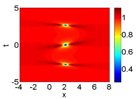
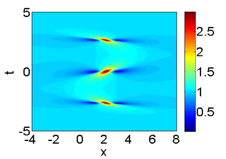
$(\rm{a})$                                                                      $(\rm{b})$

Fig. 1: Intensity of the solution (33)-(34) with $d=3\pi/4,k=\pi/4,\widetilde{d}=0,A_{0}=-2.10$ and $\nu=0.1.$ (a), (b) Dark-bright rogue waves with triple compression points in $u_{1}$ and $u_{2}$ components.

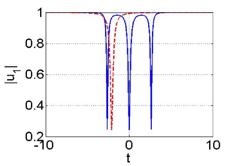
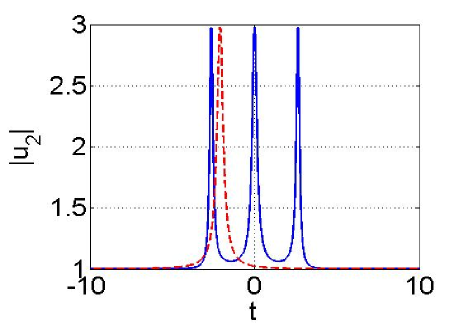
$(\rm{a})$                                                                      $(\rm{b})$

Fig. 2: Shape of the solution (33)-(34) at $x=2.11$. (a), (b) Dark-bright rogue waves with single (dashed line for $d=0$) and triple (solid line for $d=3\pi/4$) compression points. The other parameters are the same as depicted in Fig. 1.

Meanwhile, the propagation of rogue waves on periodic background can be shown by controlling the values of the constants $\widetilde{d}$ and $\widetilde{k}$. For the choice of specific parameters the intensity profiles of the dark-bright rogue waves with triple compression points under the sinusoidal wave background are exhibited in Fig. 4. The constants $\widetilde{d}$ and $\widetilde{k}$ control the amplitude and period of the background wave, respectively.

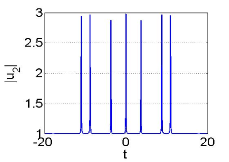
$(\rm{a})$                                                                      $(\rm{b})$

Fig. 3: (a), (b) Shape of dark-bright combs in $u_{1}$ and $u_{2}$ component with $d=15\pi/4$ at $x=2.11$. The other parameters are the same as depicted in Fig. 1.

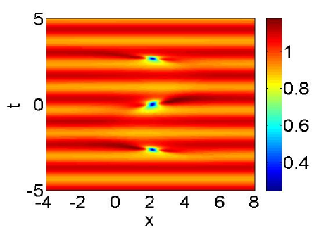
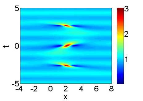
$(\rm{a})$                                                                      $(\rm{b})$

Fig. 4: Intensity of the solution (33)-(34) with $d=3\pi/4,k=\pi/4,\widetilde{d}=-0.1,\widetilde{k}=3\pi/2,A_{0}=-2.10$ and $\nu=0.1$. (a), (b) Dark-bright rogue waves with triple compression points under a sinusoidal wave background in $u_{1}$ and $u_{2}$ components.

To proceed, by returning to Eqs. (27)-(28) with $N=2$, one can compute the explicit second-order rogue wave solution. Here we refrain from writing down the cumbersome expression of the higher-order solution, and merely focus on demonstrating the complex dynamics of it. At this time, the second-order rogue waves can be classified into two types, that is, the fundamental pattern and the triangular pattern (i.e. the celebrated “three sisters” rogue wave) [10]. As before, in the light of the formula (40), by varying the amplitude of the GVD-TOD periodic modulation, the higher-order rogue waves with multiple compression points can emerge. We show that in Fig. 5(a), one dark rogue wave split into two extra peaks in the temporal direction at $t=0$ along with two normal dark rogue waves distribute with a triangle in $u_{1}$ component. Also, for the bright case in $u_{2}$ component, the analogous wave phenomenon occurs as is seen in Fig. 5(b).

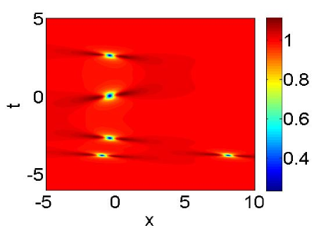
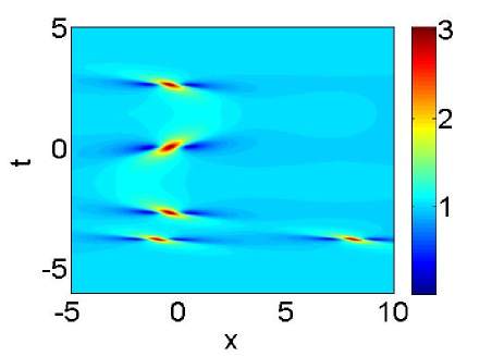
$(\rm{a})$                                                                      $(\rm{b})$

Fig. 5: Intensity of the second-order rogue wave solution given by Eqs. (27)-(28) with $N=2,d=3\pi/4,k=\pi/4,\widetilde{d}=0,m_{0}=5,m_{1}=0,n_{0}=1,n_{1}=0,A_{0}=0$ and $\nu=0.1$. (a), (b) Dark-bright three sisters involving one rogue wave with triple compression points in $u_{1}$ and $u_{2}$ components.

4.2 Composite rogue waves

By means of the formulas (31)-(32) with $N=1$, we can develop the rogue wave solution holding the form

$$u_{1}[1]=\sqrt{\dfrac{\alpha(t)}{\delta(t)}}e^{{\rm i}\theta_{1}}\dfrac{(\widetilde{G}_{1}+{\rm i}\widetilde{H}_{1})}{\widetilde{F}},$$ (41)

$$u_{2}[1]=\sqrt{\dfrac{\alpha(t)}{\delta(t)}}e^{{\rm i}\theta_{2}}\dfrac{(\widetilde{G}_{2}+{\rm i}\widetilde{H}_{2})}{\widetilde{F}},$$ (42)

where the corresponding polynomials are presented in appendix, and here we have taken $\beta(t)=\nu\alpha(t)$ with $\nu$ being a small real constant, and $m_{0}=10$, $n_{0}=0$ and $s_{0}=1/10$. At this time, it is particular to point out that the above solution is characterized by fourth degree polynomials. Consequently, there would appear composite states performing as rogue wave doublets (or rather pairs) when plotting the intensity profiles of the rogue waves described by Eqs. (41)-(42).

At this stage, as is mentioned in the above subsection, we identically select the periodic modulation functions taking the forms of Eqs. (35)-(36). Further, through the simple numerical calculations, we can infer that the maximum values of the wave amplitude in $u_{1}$ component arrive at $(x,A(t))=(14.13,0)$, $(x,A(t))=(-14.12,-0.08)$, and in $u_{2}$ component, the corresponding position coordinates are $(x,A(t))=(14.13,0)$, $(x,A(t))=(-14.00,0.08)$. In analogous to the dark-bright case, here we assume the integration constant be $A_{0}=0$. Thus, with the help of the formula (40), on can show the rogue wave doublets with multiple compression points.

As is depicted in Figs. 6, we observe that two rogue waves involving triple compression points emerge on the temporal-spacial distribution plane in $u_{1}$ and $u_{2}$ components, respectively, which is fairly different from the ordinary composite rogue waves in the coupled constant-coefficient system. Meanwhile, in the similar way, by sufficiently enlarging the value of the amplitude of periodic modulation, the comb-like rogue wave doublets with sevenfold compression points can be produced, see Fig. 7. Here it is noteworthy that we only exhibit the shape of the comb-like structure at $x=14.13$, while for $x=-14.12$ or $x=-14.00$, the situation is homologous yet the maximum values of the comb-like wave amplitudes are slightly less than that of the actual sates, and we neglect this kind of difference in the present paper.

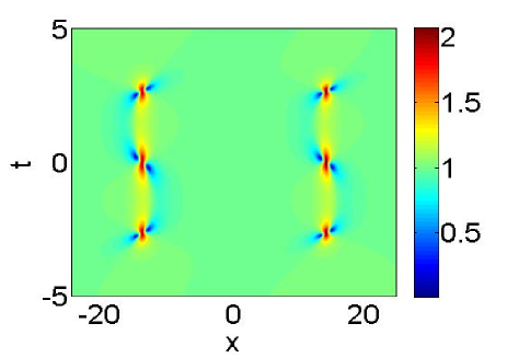
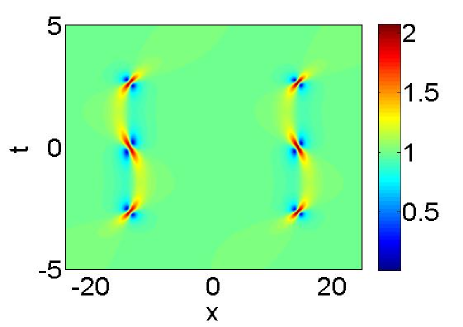
$(\rm{a})$                                                                      $(\rm{b})$

Fig. 6: Intensity of the solution (41)-(42) with $d=3\pi/4,k=\pi/4,\widetilde{d}=0,A_{0}=0$ and $\nu=0.1.$ (a), (b) Rogue wave doublets with triple compression points in $u_{1}$ and $u_{2}$ components.

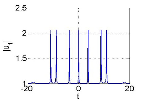
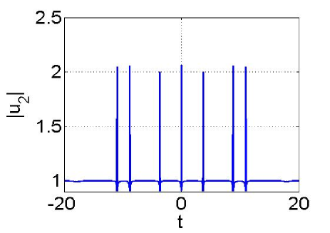
$(\rm{a})$                                                                      $(\rm{b})$

Fig. 7: (a), (b) Shape of comb doublets in $u_{1}$ and $u_{2}$ component with $d=15\pi/4$ at $x=14.13$. The other parameters are the same as depicted in Fig. 6.

Besides, as is discussed before, the rogue wave doublets with multiple compression points under periodic background can also be presented, see Fig. 8. The constants $\widetilde{d}$ and $\widetilde{k}$ play an identical part in influencing the SPM-XPM periodic modulation.

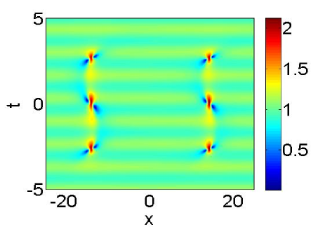
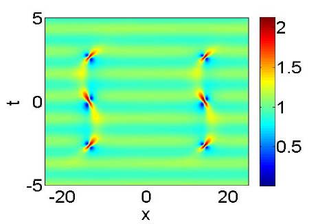
$(\rm{a})$                                                                      $(\rm{b})$

Fig. 8: Intensity of the solution (41)-(42) with $d=3\pi/4,k=\pi/4,\widetilde{d}=-0.1,\widetilde{k}=3\pi/2,A_{0}=0$ and $\nu=0.1$. (a), (b) Rogue wave doublets with triple compression points under a sinusoidal wave background in $u_{1}$ and $u_{2}$ components.

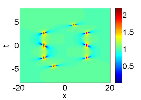
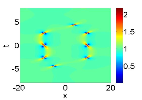
$(\rm{a})$                                                                      $(\rm{b})$

Fig. 9: Intensity of the second-order rogue wave solution given by Eqs. (31)-(32) with $N=2,d=3\pi/4,k=\pi/4,\widetilde{d}=0,m_{0}=0,m_{1}=1000,n_{0}=1,n_{1}=0,s_{0}=0,s_{1}=0,A_{0}=0$ and $\nu=0.1$. (a), (b) Rogue wave quartets involving two rogue waves with triple compression points in $u_{1}$ and $u_{2}$ components.

Ulteriorly, one can carry out the second-order rogue wave solution by means of Eqs. (31)-(32) with $N=2$. In this status, the solution is constituted by the ratio of eighth or twelfth-order polynomials. As a consequence, the higher-order rogue waves are composite of four or six fundamental rogue waves and would exhibit more abundant patterns. Naturally, for the variable-coefficient case, the corresponding rogue wave quartets or sextets involving one or more rogue waves with multiple compression points (namely, the rogue wave cluster) can arise by adjusting the values of the periodic modulation coefficients. As an example, it is vividly displayed that in Fig. 9, two rogue waves in the direction of $t=0$ separate into three compression points, together with two normal rogue waves appear with a quadrilateral in $u_{1}$ and $u_{2}$ components, respectively. In Fig. 10, we see that the rogue wave cluster including six rogue waves with triple compression points are shown. It is notable to remark that although the nonautonomous rogue wave quartets or sextets depicted in Figs. 9-10 in $u_{1}$ and $u_{2}$ components are similar, yet the concrete maximum wave amplitudes and their coordinate positions are not identical in each component.

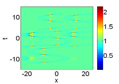
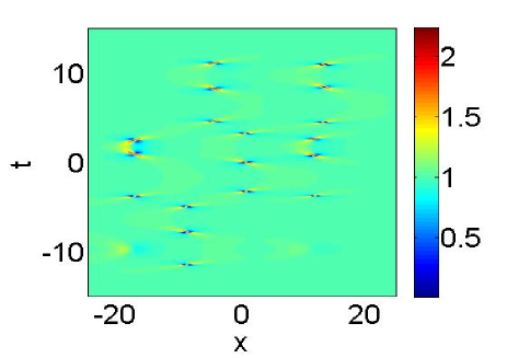
$(\rm{a})$                                                                      $(\rm{b})$

Fig. 10: Intensity of the second-order rogue wave solution given by Eqs. (31)-(32) with $N=2,d=5.8,k=\pi/4,\widetilde{d}=0,m_{0}=0,m_{1}=1000,n_{0}=0,n_{1}=0,s_{0}=0.1,s_{1}=0,A_{0}=0$ and $\nu=0.1$. (a), (b) Rogue wave cluster involving six rogue waves with triple compression points in $u_{1}$ and $u_{2}$ components.

In the last of this section, we would like to mention that the rogue wave solutions given in this paper can be reduced to the Manakov system by taking $\nu\rightarrow 0$ and $\delta(t)/\alpha(t)$ tend to a constant. On account of the presence of the higher-order effects, one can find that under identical parameter conditions compared to the Manakov system [20, 21, 22, 23], the ‘ridge’ [15, 26] of the rogue waves in Eqs. (1)-(2) is tilted to a certain extent, and the distributions of the rogue waves in t dimension is contracted significantly, see the intensity profiles in Figs. 1-10.

5 Further properties of the dark rogue wave solution

At last, let us simply discuss some wave characteristics of the interesting dark rogue wave with multiple compression points. The difference between light intensity and CW background of the nonautonomous dark rogue wave solution (33) is defined as

$$\Delta I_{c}(x,t)=|u_{1}[1]|^{2}-|u_{10}[1]|^{2},$$ (43)

where $u_{10}[1]=\displaystyle\lim_{x\rightarrow\infty}u_{1}[1]$. Hereby, we can check

$$\int_{-\infty}^{+\infty}\Delta I_{c}(x,t){\rm d}t=0,$$ (44)

which implies that for the dark rogue wave, the energy of the pump is preserved in the fiber with periodic modulation characteristics. However, it is clearly seen that in Fig. 11(a) the light intensity of the nonautonomous dark rogue wave solution is always lower than its CW background, which is different from the corresponding situation of bright case reported in [35].

Next, we can obtain the energy pulse of the nonautonomous dark rogue wave defined by

$$E_{p}(t)=\int_{-\infty}^{\infty}|u_{1}[1]-u_{10}[1]|^{2}{\rm d}t.$$ (45)

We show that the relative energy pulse is coincide well with the compression points, and with the amplitude of the periodic modulation increasing, the number of maximum points of the energy pulse also increases, see Fig. 11(b).

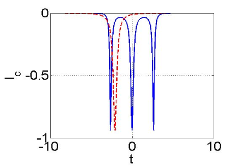
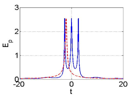
$(\rm{a})$                                                                      $(\rm{b})$

Fig. 11: (a) Shape of the difference between light intensities and CW background of the solution (33) at $x=2.11$ with $d=0$ (dashed line) and $d=3\pi/4$ (solid line); (b) Shape of the energy pulse given by (45) with $d=0$ (dashed line) and $d=3\pi/4$ (solid line). The other parameters are the same as depicted in Fig. 2.

6 Conclusion

In summary, we presented a hierarchy of rogue wave solutions under two different relative frequencies based on MI and gDT for the VCCH equations. An exact calculation formula depending on the amplitude of the periodic modulation for the number of the compression points of the rogue waves are given. Thus, the dark-bright and composite rogue waves with multiple compression points, and even the corresponding comb-like structures are generated by choosing sufficiently large periodic modulation amplitudes in coefficients of the VCCH equations. Moreover, for higher-order case, the dark-bright three sisters involving one rogue wave with triple compression points, the rogue wave quartets involving two rogue waves with triple compression points, and the rogue wave cluster involving six rogue waves with triple compression points are visually shown by selecting the adequate modulation coefficients. Further, some wave wave characteristics of the dark rogue wave solution are discussed in the last of the paper. Our work can been seen as the vector generalization with higher-order effects of Tiofack’ very recent results, and it is expected that these findings may provide some theoretical assistance to the experimental control and manipulation of vector rogue wave dynamics in inhomogeneous BEC, etc.

Appendix:Polynomials

$$G_{1}=[12x^{2}+(4\sqrt{3}z_{1}+4z_{1})x+(756\nu^{2}-72\nu z_{1}+24\sqrt{3}\nu z_{1}+48\sqrt{3})A(t)^{2}+((8\sqrt{3}z_{1}$$

$$~{}~{}~{}~{}-144\nu+24z_{1})x+360\sqrt{3}\nu-24\sqrt{3}\nu z_{1}-24\nu z_{1}+40\sqrt{3}z_{1}+120z_{1}+24)A(t)+297$$

$$~{}~{}~{}~{}+\sqrt{3}+\sqrt{3}z_{1}+3z_{1}],$$

$$H_{1}=[(6+2\sqrt{3}z_{1})x+(8\sqrt{3}z_{1}-36\nu z_{1}-12\sqrt{3}+18\nu+12z_{1}-30\sqrt{3}\nu z_{1})A(t)$$

$$~{}~{}~{}~{}+(33\sqrt{3}-29z_{1}-3-19\sqrt{3}z_{1})],$$

$$G_{2}=[12x^{2}+(4\sqrt{3}z_{1}+4z_{1})x+(756\nu^{2}-72\nu z_{1}+24\sqrt{3}\nu z_{1}+48\sqrt{3})A(t)^{2}+((8\sqrt{3}z_{1}$$

$$~{}~{}~{}~{}+24z_{1}-144\nu)x+360\nu\sqrt{3}-24\sqrt{3}\nu z_{1}-24\nu z_{1}+40\sqrt{3}z_{1}+120z_{1}+24)A(t)+297$$

$$~{}~{}~{}~{}+\sqrt{3}-\sqrt{3}z_{1}-3z_{1}],$$

$$H_{2}=[(-6+2\sqrt{3}z_{1})x-(30\sqrt{3}\nu z_{1}+36\nu z_{1}+12\sqrt{3}+8\sqrt{3}z_{1}+12z_{1}+18\nu)A(t)$$

$$~{}~{}~{}~{}-(21\sqrt{3}z_{1}+31z_{1}+27\sqrt{3}+3)],$$

$$F=2[3x^{2}+(z_{1}+\sqrt{3}z_{1})x+(189\nu^{2}-18\nu z_{1}+12\sqrt{3}+6\sqrt{3}\nu z_{1})A(t)^{2}+((6z_{1}-36\nu+2\sqrt{3}z_{1})x$$

$$~{}~{}~{}~{}+10\sqrt{3}z_{1}+30z_{1}+90\sqrt{3}\nu-6\nu z_{1}+6-6\sqrt{3}\nu z_{1})A(t)+75+\sqrt{3}],$$

$$\rho_{1}=\frac{(3+\sqrt{3}z_{1}+2z_{1})}{(6+6{\rm i}+\sqrt{3}z_{1}+z_{1}+3{\rm i}z_{1}+\sqrt{3}{\rm i}z_{1})},\ \rho_{2}=\frac{(-3+\sqrt{3}z_{1}+2z_{1})}{(-6-6{\rm i}+\sqrt{3}z_{1}+z_{1}+3{\rm i}z_{1}+\sqrt{3}{\rm i}z_{1})},$$

$$\widetilde{G}_{1}=2304x^{4}+4608\sqrt{3}x^{3}-932352x^{2}-920576\sqrt{3}x+81(363\nu^{2}+16)^{2}A(t)^{4}+(-14256\nu(363\nu^{2}$$

$$~{}~{}~{}~{}+16)x-216\sqrt{3}(192+16335\nu^{3}+4356\nu^{2}+1040\nu))A(t)^{3}+((940896\nu^{2}+13824)x^{2}$$

$$~{}~{}~{}~{}+288\sqrt{3}(4059\nu^{2}+112+792\nu)x-124416\nu-63053856\nu^{2}+2797056)A(t)^{2}+(-76032\nu x^{3}$$

$$~{}~{}~{}~{}-3456\sqrt{3}(37\nu+4)x^{2}+15342336\nu x+768\sqrt{3}(-3576+13507\nu))A(t)+93077504,$$

$$\widetilde{H}_{1}=-2304\sqrt{3}x^{4}+4608x^{3}+923136\sqrt{3}x^{2}-930816x-81\sqrt{3}(363\nu^{2}+16)^{2}A(t)^{4}$$

$$~{}~{}~{}~{}+(14256\sqrt{3}\nu(363\nu^{2}+16)x+235224\nu^{3}-41472-940896\nu^{2}+217728\nu)A(t)^{3}$$

$$~{}~{}~{}~{}+(-864\sqrt{3}(1089\nu^{2}+16)x^{2}+(228096\nu+256608\nu^{2}-41472)x+288\sqrt{3}(-9488+384\nu$$

$$~{}~{}~{}~{}+218343\nu^{2}))A(t)^{2}+(76032\sqrt{3}\nu x^{3}-(72576\nu+13824)x^{2}-2304\sqrt{3}(8+6617\nu)x$$

$$~{}~{}~{}~{}-2783232-573696\nu)A(t)-91238400\sqrt{3},$$

$$\widetilde{G}_{2}=2304x^{4}+4608\sqrt{3}x^{3}-932352x^{2}-920576\sqrt{3}x+81(363\nu^{2}+16)^{2}A(t)^{4}+(-14256\nu(363\nu^{2}$$

$$~{}~{}~{}~{}+16)x-216\sqrt{3}(-192-4356\nu^{2}+1040\nu+16335\nu^{3}))A(t)^{3}+((940896\nu^{2}+13824)x^{2}$$

$$~{}~{}~{}~{}+288\sqrt{3}(112+4059\nu^{2}-792\nu)x+124416\nu-63053856\nu^{2}+2797056)A(t)^{2}+(-76032\nu x^{3}$$

$$~{}~{}~{}~{}-3456\sqrt{3}(37\nu-4)x^{2}+15342336\nu x+768\sqrt{3}(13507\nu+3576))A(t)+93077504,$$

$$\widetilde{H}_{2}=2304\sqrt{3}x^{4}-4608x^{3}-923136\sqrt{3}x^{2}+930816x+81\sqrt{3}(363\nu^{2}+16)^{2}A(t)^{4}$$

$$~{}~{}~{}~{}+(-14256\sqrt{3}\nu(363\nu^{2}+16)x-235224\nu^{3}-41472-940896\nu^{2}-217728\nu)A(t)^{3}$$

$$~{}~{}~{}~{}+(864\sqrt{3}(1089\nu^{2}+16)x^{2}+(228096\nu-256608\nu^{2}+41472)x-288\sqrt{3}(-9488-384\nu$$

$$~{}~{}~{}~{}+218343\nu^{2}))A(t)^{2}+(-76032\sqrt{3}\nu x^{3}+(72576\nu-13824)x^{2}+2304\sqrt{3}(-8+6617\nu)x$$

$$~{}~{}~{}~{}-2783232+573696\nu)A(t)+91238400\sqrt{3},$$

$$\widetilde{F}=-4608x^{4}+1837056x^{2}+4096\sqrt{3}x-162(363\nu^{2}+16)^{2}A(t)^{4}+(28512\nu(363\nu^{2}+16)x$$

$$~{}~{}~{}~{}+1728\sqrt{3}\nu(128+1089\nu^{2}))A(t)^{3}+((-1881792\nu^{2}-27648)x^{2}-4608\sqrt{3}(99\nu^{2}+8)x$$

$$~{}~{}~{}~{}+124910208\nu^{2}-5566464)A(t)^{2}+(152064\nu x^{3}+27648\sqrt{3}\nu x^{2}-30311424\nu x$$

$$~{}~{}~{}~{}-5563392\sqrt{3}\nu)A(t)-184324096.$$

References

References

• [1] C. Kharif and E. Pelinovsky, Physical mechanisms of the rogue wave phenomenon, Eur. J. Mech. B Fluids 22, 603-34 (2003).
• [2] K. Dysthe, H.E Krogstad and P. Müller, Oceanic rogue waves, Annu. Rev. Fluid Mech. 40, 287-310 (2008).
• [3] D.R. Solli, C. Ropers, P. Koonath and B. Jalali, Optical rogue waves, Nature 450, 1054-7 (2007).
• [4] Y.V. Bludov, V.V. Konotop and N. Akhmediev, Matter rogue waves, Phys. Rev. A 80 033610 (2009).
• [5] L. Stenflo and M. Marklund, Rogue waves in the atmosphere, J. Plasma Phys. 76 293-5 (2010).
• [6] W.M. Moslem, P.K. Shukla and B. Eliasson, Surface plasma rogue waves, Eur. Phys. Lett. 96 25002 (2011).
• [7] Z.Y. Yan, Financial rogue waves, Commun. Theor. Phys. 54 947-9 (2010).
• [8] N. Akhmediev, A. Ankiewicz and M. Taki, Waves that appear from nowhere and disappear without a trace, Phys. Lett. A 373 675-8 (2009).
• [9] D.H. Peregrine and J. Austral, Water waves, nonlinear Schrödinger equations and their solutions, Math. Soc. B: Appl. Math. 25 16-43 (1983).
• [10] A. Ankiewicz, D.J. Kedziora and N. Akhmediev, Rogue wave triplets, Phys. Lett. A 375 2782-5 (2011).
• [11] D.J. Kedziora, A. Ankiewicz and N. Akhmediev, Circular rogue wave clusters, Phys. Rev. E 84 056611 (2011).
• [12] D.J. Kedziora, A. Ankiewicz and N. Akhmediev, Classifying the hierarchy of nonlinear-Schrödinger-equation rogue-wave solutions, Phys. Rev. E 88 013207 (2013).
• [13] A. Chabchoub, N.P. Hoffmann and N. Akhmediev, Rogue wave observation in a water wave tank, Phys. Rev. Lett. 106 204502 (2011).
• [14] A. Chabchoub, N. Hoffmann, M. Onorato, Slunyaev, el al., Observation of a hierarchy of up to fifth-order rogue waves in a water tank, Phys. Rev. E 86 056601 (2012).
• [15] A. Ankiewicz, J.M. Soto-Crespo and N. Akhmediev, Rogue waves and rational solutions of the Hirota equation, Phys. Rev. E 81 046602 (2010).
• [16] L.H. Wang, K. Porsezian and J.S. He, Breather and rogue wave solutions of a generalized nonlinear Schrödinger equation, Phys. Rev. E 87 053202 (2013)
• [17] A. Ankiewicz, Y. Wang, S. Wabnitz and N. Akhmediev, Extended nonlinear Schrödinger equation with higher-order odd and even terms and its rogue wave solutions, Phys. Rev. E 89 012907 (2014).
• [18] X. Wang, B. Yang, Y. Chen and Y.Q. Yang, Higher-order rogue wave solutions of the Kundu-Eckhaus equation, Phys. Scr. 89 095210 (2014).
• [19] F. Baronio, A. Degasperis, M. Conforti and S. Wabnitz, Solutions of the vector nonlinear Schrödinger equations: evidence for deterministic rogue waves, Phys. Rev. Lett. 109 044102 (2012).
• [20] L.C. Zhao and J. Liu, Localized nonlinear waves in a two-mode nonlinear fiber, J. Opt. Soc. Am. B 29 3119-27 (2012).
• [21] L.M. Ling, B.L. Guo and L.C. Zhao, High-order rogue waves in vector nonlinear Schrödinger equations, Phys. Rev. E 89 041201 (2014).
• [22] S.H. Chen and L.Y. Song, Rogue waves in coupled Hirota systems, Phys. Rev. E 87 032910 (2013).
• [23] S.H. Chen, Dark and composite rogue waves in the coupled Hirota equations, Phys. Lett. A 378 2851-6 (2014).
• [24] X. Wang, Y.Q. Li and Y. Chen, Generalized Darboux transformation and localized waves in coupled Hirota equations, Wave Motion 51 1149-60 (2014).
• [25] F. Baronio, M. Conforti, A. Degasperis and S. Lombardo, Rogue waves emerging from the resonant interaction of three waves, Phys. Rev. Lett. 111 114101 (2013).
• [26] L.J. Li, Z.W. Wu, L.H. Wang and J.S. He, High-order rogue waves for the Hirota equation, Ann. Phys. 334 198-211 (2013).
• [27] A. Chowdury, D.J. Kedziora, A. Ankiewicz and N. Akhmediev, Breather-to-soliton conversions described by the quintic equation of the nonlinear Schrödinger hierarchy, Phys. Rev. E 91 032928 (2015).
• [28] C. Liu, Z.Y. Yang , L.C. Zhao and W.L. Yang, Transition, coexistence, and interaction of vector localized waves arising from higher-order effects, Ann. Phys. 362 130-8 (2015).
• [29] L.C. Zhao and J. Liu, Rogue-wave solutions of a three-component coupled nonlinear Schrödinger equation, Phys. Rev. E 87 013201 (2013).
• [30] S. Loomba, H. Kaur, R. Gupta, C.N. Kumar, et al., Controlling rogue waves in inhomogeneous Bose-Einstein condensates, Phys. Rev. E, 89 052915 (2014).
• [31] Z.Y. Yan and C.Q. Dai, Optical rogue waves in the generalized inhomogeneous higher-order nonlinear Schrödinger equation with modulating coefficients, J. Opt. 15 064012 (2013).
• [32] S. Loomba, R. Pal and C.N. Kumar, Bright solitons of the nonautonomous cubic-quintic nonlinear Schröodinger equation with sign-reversal nonlinearity, Phys. Rev. E 92 033811 (2015).
• [33] W.P. Zhong, M. Belić and B.A. Malomed, Rogue waves in a two-component Manakov system with variable coefficients and an external potential, Phys. Rev. E 92 053201 (2015).
• [34] L. Wang, X. Li, F.H. Qi and L.L. Zhang, Breather interactions and higher-order nonautonomous rogue waves for the inhomogeneous nonlinear Schrödinger Maxwell-Bloch equations, Ann. Phys. 359 97-114 (2015).
• [35] C.G.L. Tiofack, S. Coulibaly and M. Taki, Comb generation using multiple compression points of Peregrine rogue waves in periodically modulated nonlinear Schrödinger equations, Phys. Rev. A 92 043837 (2015).
• [36] R.S. Tasgal and M. J. Potasek, Soliton solutions to coupled higher-order nonlinear Schrödinger equations, J. Math. Phys. 33 1208-15 (1992).
• [37] J.S. He, Y.S. Tao, K. Porsezian and A.S. Fokas, Rogue wave management in an inhomogeneous Nonlinear Fibre with higher order effects, J. Nonlinear Math. Phys. 20 407-19 (2013).
• [38] L.C. Zhao, G.G. Xin and Z.Y. Yang, Rogue-wave pattern transition induced by relative frequency, Phys. Rev. E 90 022918 (2014).
• [39] B.L. Guo, L.M. Ling and Q.P. Liu, Nonlinear Schrödinger equation: Generalized Darboux transformation and rogue wave solutions, Phys. Rev. E 85 026607 (2012).
• [40] B.L. Guo, L.M. Ling and Q.P. Liu, High-Order solutions and generalized Darboux transformations of derivative nonlinear Schrödinger Equations, Stud. Appl. Math. 130 317-44 (2013).
• [41] Zhaqilao, On Nth-order rogue wave solution to the generalized nonlinear Schrödinger equation, Phys. Lett. A 377 855-9 (2013).
• [42] N.V. Priya and M. Senthilvelan, Generalized Darboux transformation and Nth order rogue wave solution of a general coupled nonlinear Schrödinger equations, Commun. Nonlinear Sci. Numer. Simul. 20 401-20 (2015).
• [43] X. Wang, Y.Q. Li, F. Huang and Y. Chen, Rogue wave solutions of AB system, Commun. Nonlinear Sci. Numer. Simul. 20 434-42 (2015).