Probing phase transition order of -state Potts models using Wang-Landau Algorithm
Abstract
Phase transitions are ubiquitous phenomena, exemplified by the melting of ice and spontaneous magnetization of magnetic material. In general, a phase transition is associated with a symmetry breaking of a system; occurs due to the competition between coupling interaction and external fields such as thermal energy. If the phase transition occurs with no latent heat, the system experiences continuous transition, also known as second order phase transition. The ferromagnetic -state Potts model with extra invisible states, introduced by Tamura, Tanaka, and Kawashima [Prog. Theor. Phys. 124, 381 (2010)], is studied by using the Wang-Landau method. The density of states difference (DOSD), , is used to investigate the order of the phase transition and examine the critical value of changing the second to the first order transition.
pacs:
05.50.+q, 75.40.Mg, 05.10.Ln, 64.60.DeI Introduction
The study of phase transitions has been one of the main subjects in physics since the introduction of the Ising model Ising mainly aimed to explain the phenomenon of spontaneous magntization in ferromagnet (FM). In general, a phase transition is associated with a symmetry breaking Landau ; occurs due to the competition between coupling interaction and thermal energy. Systems are in high degree of symmetry at high temperature because all configurational spaces are accessible. The decrease in temperature will reduce thermal fluctuation and the system will stay in some favorable states. If the phase transition occurs with no latent heat, the system experiences continuous transition, also known as second order phase transition, which is a transition between the ordered and the disordered state.
The order of phase transition of a system is frequently not quite obvious and sometimes becomes a subject of debate. In this paper, we focus on the phase transition of -state Potts model. It is a magnetic model applicable to many physical systems such as polycrystalline material, simple fluids, percolation problems, etc.Potts This model is a generalization of Ising model which is known to exhibit second order phase transition for -dimensional case, with .
The order of phase transition of -state Potts models varies with and the spatial dimensions as well as the spin coupling interaction. It is well known that the two-dimensional (2D) FM case of the model experiences second order phase transition for , and first order for otherwise. In 3D case, the model experiences first order transition for . The anti-ferromagnetic (AF) Potts model is considered to be more complex than the FM case as its behaviour depends strongly on the microscopic lattice structure. A systematic study of 3D AF case by Yamaguchi and Okabe reported that the phase transition is second order for and . There exists zero temperature transition for and for no order found at any temperatures Yamaguchi .
Recently, Tamura et al. studied -state Potts, which is a -state Potts model with invisible redundant statesTamura . The invisible states of the model affect the entropy but do not contribute to the internal energy. Although this model is a straightforward extension of the standard ferromagnetic Potts model, due to the effect of invisible states, a spontaneous fold symmetry breaking of a first order phase transition can occur in 2D case for , and . For each , there is a critical value of which can change the second order transition of the corresponding standard -state Potts model into a first order. Thus, it is of theoretical interest to determine this critical value of .
Several methods are used for the analysis of phase transition. An example of this is the usage of probability distribution function combined with the histogram reweighting for the analysis of first-order transition. For this type of transition, the multicanonical Monte Carlo method calculating the energy density of states (DOS) was shown to be effective Berg . Quite recently, Komura and Okabe Komura studied the difference of DOS, , and examined the behavior of the first-order transition with this quantity in connection with Maxwell’s equal area rule. The paper elaborates the analysis of the density of state difference (DOSD) obtained from Wang-Landau algorithm Wang in determining the order of phase transition of the 2D -state Potts model. The remaining part of the paper is organized as follows: Section II describes the model and the method. The result is discussed in Section III. Section IV is devoted to the summary and concluding remark.
II Model and Simulation Method
The -state Potts model is written with the following Hamiltonian
| (1) |
For any spin configuration, the Potts spin on site i- can take one of states, with and are respectively referred to as colored states and invisible states. The standard Potts models is recovered if . Summation is performed over all the nearest-neighbor pairs of spins on a square lattice with ferromagnetic interaction () and with periodic boundary condition. If two neighboring spins take the same state, then the energy coupling is , otherwise it becomes zero. It is to be noticed that even if two neighboring spins are equal, the energy remains zero if spins are in invisible state, i.e., . Therefore, the ground state energy is with is the number of spins.
Monte Carlo simulation is a standard method used in many field of physics, including the study of phase transition of magnetic models. Here, we use Wang-Landau algorithm to calculate the DOS of the models. This algorithm is particularly powerful for this purpose. It has been implementend in various type of systems, such AF Potts model Yamaguchi and fully frustrated Clock model Tasrief04 . From the calculated DOS , we can straightforward obtain DOSD defined as
| (2) |
For the considered model, , and the total energy takes the value between and , where is the number of spins. However, for the convenience of the numerical simulation, we shifted the energy so that it takes the value between and . A general procedure of determining the order of transition using DOSD was described by Komura and Okabe Komura . It was shown that a system exhibiting first-order transition will have an S-like structure in the plot of . The transition temperature of this type of transition can be determined using Maxwell’s equal area rule.
III Results and Discussion
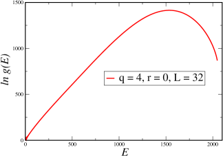
As has been described, the 2D -state Potts model undergoes second-order phase transition for and first order for otherwise. We should show this behaviour using DOSD before presenting the results for -state Potts model. The DOS of standard -state Potts model for is plotted in Fig. 1. This type of figure is typical of DOS in regular magnetic systems where density of ground state is much less than that of excited states. Obtaining the data of any physical quantity for every state, expressed as which can be referred as to density of quantity, we can calculate ensemble average via the following relation
| (3) |
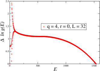
This equation implies the forthcoming of Wang-Landau algorithm as one can obtain the value of at any temperature. In addition, from the same data of simulation one can obtain by-product results for anti-ferromagnetic system, namely by changing the energy into . This is demonstrated in the study of ferromagnetic -state Clock model for various 2D lattices Tasrief13 . From the data of DOS, shown in Fig. 1, we extract the DOSD of the corresponding model and system size, (See. Fig. 2). Throughout, the energy is in unit of and the Boltzmann constant is set as 1.
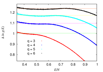
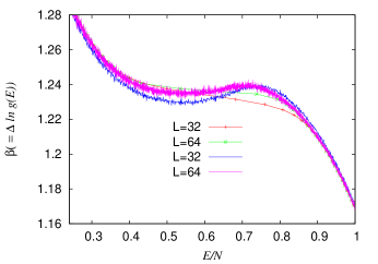
The DOSD of standard -state Potts model for several values of ( and ) are plotted in Fig. 3. The linear system size is . In order to reduce fluctuations, in plotting we use the data with the smoothing process, with .
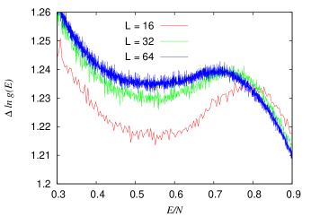
The S-like structure for in Fig. 3 is the indication of first order transition. The inverse transition temperature can be estimated by Maxwell’s equal area rule as described in Ref. Komura . For convenience, it is also shown in the thermodynamic limit . We plot for the -state Potts model for various sizes in Fig. 4, which shows size dependence; the S-like structure becomes smaller when the system size increases.
Let us examine the meaning of . This quantity is related to the inverse of temperature in the microcanonical scheme where we have
| (4) |
in the continuum limit. We note that in the present model. The plot of as a function of as in Fig. 4 is nothing but versus plot; it is to be noted that for discrete energy models such as the Potts model there is an oscillating behavior for low DOS region due to the discreteness as was shown in Fig. 1 of Ref. Komura . It is interesting to compare this with the temperature dependence of the ensemble average of energy, following definition of Eq. (3)
In Fig. 5, we compare plot of versus and plot of versus for the -state Potts model, with system size and . The S-like structure shown by solid curve, in the microcanonical scheme leads to the negative specific heat, or the thermodynamic instability. Then, the canonical average of energy, which is shown by dotted curve, has a jump at the first-order transition temperature due to Maxwell’s equal area rule. When the system size increases from 32 to 64, the behavior of S-like structure approaches that of the thermodynamic limit; that is, the line to express the energy jump becomes horizontal. Away from the first-order transition temperature, two curves coincide with each other as the system size increases.
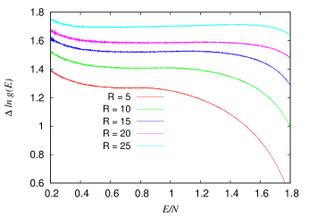
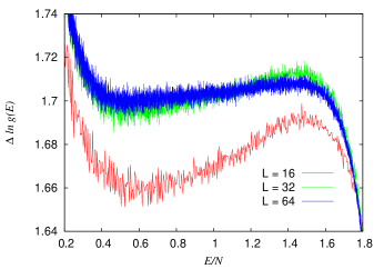
We plot the DOSD for the -state Potts model of system size , with and in Fig. 6. As indicated, there is an S-like structure for , whereas there is no such a structure for . The intermediate behavior is for . To see the size dependence carefully, we plot the size dependence of for and , as a typical example for the first-order transition, in Fig. 7.
We can estimate and the interfacial free energy from the S-like curve for each size. The procedure for estimating the transition temperature and the interfacial free energy is the same as that for the -state Potts model Berg . The numerically exact estimate of the interfacial free energy for the q-state Potts model was made by Borgs and Janke Jangke . The detail analysis of obtaining these quantities for -state Potts model will be reported elsewhere.
IV Summary and Concluding Remarks
In summary, we have studied the -state Potts model with and without invisible states and demonstrated the implementation of the density of states difference (DOSD) extracted from the main result of Wang-Landau Algorithm in examining the order of phase transition. We have obtained deeper understanding of the role of redundant states in the -state Potts model, namely transforming the second order into first order phase transition at critical value of . For for example, the critical value for is around 20. There are several models where the order of the transition changes with some parameter, for example, the modified XY model Domany . It will be interesting to study the change of the order of transitions for these models using the present method of analyzing the density of states difference.
Acknowledgments
The authors wish to thank Terry Mart, Bansawang BJ and Safaruddin A. Prasad for valuable discussions. The extensive computation was performed using the parallel computer facilities of the Department of Physics, Hasanuddin University and that of Tokyo Metropolitan University, JAPAN. The present work is financially supported by Research Grant of BOPTN of Hasanuddin University, FY 2013.
References
- (1) E. Ising, Z. Phys., 31, 253, (1925).
- (2) L. D. Landau, On the theory of phase transition, in Collected Papers of L. D. Landau, edited by D. T. Haar (Pergamon Press, 1965).
- (3) R. B. Potts, Proc. Cambridge. Philos. Soc. 48, 106 (1952); F. Y. Wu, Rev. Mod. Phys. 54, 235 (1982).
- (4) C. Yamaguchi and Y.Okabe, J. Phys. A 34, 8781 (2001)
- (5) R. Tamura, S. Tanaka, and N. Kawashima, Prog. Theor. Phys. 124, 381 (2010).
- (6) B. A. Berg and T. Neuhaus, Phys. Rev. Lett. 68, 9 (1992).
- (7) Y. Komura and Y. Okabe, Phys. Rev. E 85, 010102(R) (2012).
- (8) T. Surungan, in preparation.
- (9) F. Wang and D.P. Landau, Phys. Rev. Lett. 86, 2050 (2001); Phys. Rev. E 64, 056101 (2001).
- (10) T. Surungan, Y. Okabe, and Y. Tomita, J. Phys. A 37, 4219 (2004).
- (11) W. Janke, Phys. Rev. B 47, 14757 (1993); C. Borgs and W. Janke, J. Phys. (France) I 2, 2011 (1992).
- (12) E. Domany, M.Schick, and R.H. Swendsen, Phys. Rev. Lett. 52, 1535 (1984).