The Lovász Hinge: A Novel Convex Surrogate for Submodular Losses

Abstract

Learning with non-modular losses is an important problem when sets of predictions are made simultaneously. The main tools for constructing convex surrogate loss functions for set prediction are margin rescaling and slack rescaling. In this work, we show that these strategies lead to tight convex surrogates iff the underlying loss function is increasing in the number of incorrect predictions. However, gradient or cutting-plane computation for these functions is NP-hard for non-supermodular loss functions. We propose instead a novel surrogate loss function for submodular losses, the Lovász hinge, which leads to $\mathcal{O}(p\log p)$ complexity with $\mathcal{O}(p)$ oracle accesses to the loss function to compute a gradient or cutting-plane. We prove that the Lovász hinge is convex and yields an extension. As a result, we have developed the first tractable convex surrogates in the literature for submodular losses. We demonstrate the utility of this novel convex surrogate through several set prediction tasks, including on the PASCAL VOC and Microsoft COCO datasets.

1 Introduction

Statistical learning has largely addressed problems in which a loss function decomposes over individual training samples. However, there are many circumstances in which non-modular losses must be minimized. This is the case when multiple outputs of a prediction system are used as the basis of a decision making process that leads to a single real-world outcome. These dependencies in the effect of the predictions (rather than a statistical dependency between predictions themselves) are therefore properly incorporated into a learning system through a non-modular loss function. In this paper, we aim to provide a theoretical and algorithmic foundation for a novel class of learning algorithms that make feasible learning with submodular losses, an important subclass of non-modular losses that is currently infeasible with existing algorithms. This paper provides a unified and extended presentation of our conference paper [1].

Convex surrogate loss functions are central to the practical application of empirical risk minimization. Straightforward principles have been developed for the design of convex surrogates for binary classification and regression [2], and in the structured output setting margin and slack rescaling are two principles for defining convex surrogates for more general output spaces [3]. Despite the apparent flexibility of margin and slack rescaling in their ability to bound arbitrary loss functions, there are fundamental limitations to our ability to apply these methods in practice: (i) they provide only loose upper bounds to certain loss functions (cf. Propositions 1 & 2), (ii) computing a gradient or cutting plane is NP-hard for submodular loss functions, and (iii) consistency results are lacking in general [4, 5]. In practice, modular losses, such as Hamming loss, are often applied to maintain tractability, although non-modular losses, such as the Jaccard loss have been applied in the structured prediction setting [6, 7]. We show in this paper that the Jaccard loss is in fact a submodular loss, and our proposed convex surrogate provides a polynomial-time tight upper bound.

Non-modular losses have been (implicitly) considered in the context of multilabel classification problems. [8] uses the Hamming loss and subset 0-1 loss which are modular, and a rank loss which is supermodular; [9] introduces submodular pairwise potentials, not submodular loss functions, while using a non-submodular loss based on F-score. [10] uses (weighted) Hamming loss which is modular, but also proposes a new tree-based algorithm for training; [11] uses modular losses e.g. Hamming loss and F1 loss which is non-submodular. If the relevant loss at test time is non-modular, it is essential to optimize the correct loss during training time [12, 13]. However, non-supermodular loss functions are substantially more rare in the literature.

In this work, we introduce an alternate principle to construct convex surrogate loss functions for submodular losses based on the Lovász extension of a set function. The Lovász extension of a submodular function is its convex closure, and has been used in other machine learning contexts e.g. [14, 15]. We analyze the settings in which margin and slack rescaling are tight convex surrogates by finding necessary and sufficient conditions for the surrogate function to be an extension of a set function. Although margin and slack rescaling generate extensions of some submodular set functions, their optimization is NP-hard. We therefore propose a novel convex surrogate for submodular functions based on the Lovász extension, which we call the Lovász hinge. In contrast to margin and slack rescaling, the Lovász hinge provides a tight convex surrogate to all submodular loss functions, and computation of a gradient or cutting plane can be achieved in $\mathcal{O}(p\log p)$ time with a linear number of oracle accesses to the loss function. We demonstrate empirically fast convergence of a cutting plane optimization strategy applied to the Lovász hinge, and show that optimization of a submodular loss results in lower average loss on the test set.

In Section 2 we introduce the notion of a submodular loss function in the context of empirical risk minimization. The Structured Output SVM is one of the most popular objectives for empirical risk minimization of interdependent outputs, and we demonstrate its properties on non-modular loss functions in Section 3. In Section 4 we introduce the Lovász hinge as well as properties involving the convexity and computational complexity. We empirically demonstrate its performance first on a synthetic problem, then on image classification and labeling tasks on Pascal VOC dataset and the Microsoft COCO dataset in Section 6.

2 Submodular Loss Functions

In empirical risk minimization, we approximate the risk, $\mathcal{R}$ of a prediction function $f:\mathcal{X}\mapsto\mathcal{Y}$ by an empirical sum over losses incurred on a finite sample, using e.g. an i.i.d. sampling assumption [16]:

$$\hat{\mathcal{R}}(f):=\frac{1}{n}\sum_{i=1}^{n}\Delta(y_{i},f(x_{i}))$$ (1)

Central to the practical application of the empirical risk minimization principle, one must approximate, or upper bound the discrete loss function $\Delta$ with a convex surrogate. We will identify the creation of a convex surrogate for a specific loss function with an operator that maps a function with a discrete domain to one with a continuous domain. In particular, we will study the case that the discrete domain is a set of $p$ binary predictions. In this case we denote

$$\mathcal{Y} =\{-1,+1\}^{p}$$ (2)

$$\Delta :\mathcal{Y}\times\mathcal{Y}\mapsto\mathbb{R}_{+}$$ (3)

$$\mathbf{B}\Delta :\mathcal{Y}\times\mathbb{R}^{p}\mapsto\mathbb{R}$$ (4)

where $\mathbf{B}$ is an operator that constructs the surrogate loss function from $\Delta$, and we assume

$$f(x)=\operatorname{sign}(g(x))$$ (5)

where $g:\mathcal{X}\mapsto\mathbb{R}^{p}$ is a parametrized prediction function to be optimized by empirical risk minimization.

A key property is the relationship between $\mathbf{B}\Delta$ and $\Delta$. In particular, we are interested in when a given surrogate strategy $\mathbf{B}\Delta$ yields an extension of $\Delta$ (cf. Definition 3). We make this notion formal by identifying $\{-1,+1\}^{p}$ with a given $p$-dimensional unit hypercube of $\mathbb{R}^{p}$ . We say that $\mathbf{B}\Delta(y,\cdot)$ is an extension of $\Delta(y,\cdot)$ iff the functions are equal over the vertices of this unit hypercube. We focus on function extensions as they ensure a tight relationship between the discrete loss and the convex surrogate.

2.1 Set Functions and Submodularity

For many optimization problems, a function defined on the power set of a given base set $V=\{1,\cdots,p\}$ ($p=|V|$), a set function is often taken into consideration to be minimized (or maximized). Submodular functions play an important role among these set functions, similar to convex functions on vector spaces.

Submodular functions may be defined through several equivalent properties. We use the following definition [17]:

Definition 1.

A set function $l:\mathcal{P}(V)\mapsto\mathbb{R}$ is submodular if for all subsets $A,B\subseteq V$, it holds

$$l(A)+l(B)\geq l(A\cup B)+l(A\cap B).$$ (6)

An equivalent definition known as the diminishing returns property follows: for all $B\subseteq A\subset V$ and $x\in V\setminus B$, it holds

$$l(B\cup\{x\})-l(B)\geq l(A\cup\{x\})-l(A)$$ (7)

A function is supermodular if its negative is submodular, and a function is modular if it is both submodular and supermodular. A modular function can be written as a dot product between a binary vector in $\{0,1\}^{p}$ encoding a subset of $V$ and a coefficient vector in $\mathbb{R}^{p}$ which uniquely identifies the modular function. By example, Hamming loss is a modular function with a coefficient vector of all ones, and a subset defined by the entries that differ between two vectors.

Necessary to the sequel is the notion of monotone set functions

Definition 2.

A set function $l:\mathcal{P}(V)\mapsto\mathbb{R}$ is increasing if for all subsets $A\subset V$ and elements $x\in V\setminus A$, it holds

$$l(A)\leq l(A\cup\{x\}).$$ (8)

In this paper, we consider loss functions for multiple outputs that are set functions where inclusion in a set is defined by a corresponding prediction being incorrect:

$$\Delta(y,\tilde{y})=l(\{i|y^{i}\neq\tilde{y}^{i}\})$$ (9)

for some set function $l$. For a given groundtruth $y$, $(y,\tilde{y})\rightarrow A:=\{i|y^{i}\neq\tilde{y}^{i}\}$, $\Delta(y,\tilde{y})\cong l(A)$ is an isomorphism. In the sequel when we say $\Delta$ is increasing we mean it is increasing w.r.t. the misprediciton set $\{i|y^{i}\neq\tilde{y}^{i}\}$. Such functions are typically increasing, though it is possible to conceive of a sensible loss function that may not be increasing (e.g. when getting 50% recall is worse than making no prediction at all, as in the identification of cancer tissue).

With these notions, we now turn to an analysis of margin and slack rescaling, and show necessary and sufficient conditions for these operators to yield an extension to the underlying discrete loss function.

3 Existing Convex Surrogates

In this section, we analyze two existing convex surrogates namely margin rescaling and slack rescaling. We determine necessary and sufficient conditions for margin and slack rescaling to yield an extension of the underlying set loss function, and address their shortcoming in the complexity of subgradient computation.

A general problem is to learn a mapping $f$ from inputs $x\in\mathcal{X}$ to discrete outputs (labels) $y\in\mathcal{Y}$. The Structured Output SVM (SOSVM) is a popular framework for doing so in the regularized risk minimization framework [18, 3]. The approach that SOSVM pursues is to learn a function $h:\mathcal{X}\times\mathcal{Y}\mapsto\mathbb{R}$ over input/output pairs from which a prediction can be derived by maximizing

$$f(x)=\arg\max_{y}h(x,y)$$ (10)

over the response from a given input $x$. The SOSVM framework assumes $h$ to be represented by an inner product between an element of a reproducing kernel Hilbert space and some combined feature representation of inputs and outputs $\phi(x,y)$,

$$h(x,y;w)=\langle w,\phi(x,y)\rangle$$ (11)

although the notions of margin and slack rescaling may be applied to other function spaces, including random forests [19] and deep networks [20].

A bounded loss function $\Delta:\mathcal{Y\times Y}\to\mathbb{R}$ quantifies the loss associated with a prediction $\tilde{y}$ while the true value is $y$, and is used to re-scale the constraints. The parameters are estimated by solving the following optimization problem, with the margin-rescaling constraints and slack-rescaling constraints in Equation (13) and Equation (14), respectively:

$$\min_{w,\xi}\frac{1}{2}\|w\|^{2}+C\sum_{i=1}^{n}\xi_{i},\quad\forall i,\forall\tilde{y}\in\mathcal{Y}:$$ (12)

$$\langle w,\phi(x_{i},y_{i})\rangle-\langle w,\phi(x_{i},\tilde{y})\rangle\geq\Delta(y_{i},\tilde{y})-\xi_{i}\quad\text{or}$$ (13)

$$\Delta(y_{i},\tilde{y})\left(\langle w,\phi(x_{i},y_{i})\rangle-\langle w,\phi(x_{i},\tilde{y})\rangle\right)\geq\Delta(y_{i},\tilde{y})-\xi_{i}.$$ (14)

A cutting plane algorithm is commonly used to solve it and one version of the approach with slack rescaling is shown in Algorithm 1.

Algorithm 1 Cutting plane algorithm for solving the problem in Equation (12) and (14) – Slack rescaling.

1:  Input: $(x_{1},y_{1}),\cdots,(x_{n},y_{n}),C,\epsilon$

2:  $S^{i}=\emptyset,\forall i=1,\cdots,n$

3:  repeat

4:     for $i=1,\cdots,n$ do

5:        $\hat{y}=\arg\max_{\tilde{y}}H(y_{i},\tilde{y}_{i})=\arg\max_{\tilde{y}}\Delta(y_{i},\tilde{y})(1+h(x,\tilde{y})-h(x,y_{i}))$ % most violated constraint

6:        $\xi^{i}=\max\{0,H(y_{i},\hat{y}_{i})\}$

7:        if $H(y_{i},\hat{y}_{i})>\xi^{i}+\epsilon$  then

8:           $S^{i}:=S^{i}\cup\{\hat{y}_{i}\}$

9:           $w\leftarrow$ optimize Equation (12) with constraints defined by $\cup_{i}S^{i}$

10:        end if

11:     end for

12:  until no $S^{i}$ has changed during an iteration

13:  return  $(w,\xi)$

In the sequel, we will consider the case that each $x_{i}\in\mathcal{X}$ is an ordered set of $p$ elements, and that $y_{i}\in\mathcal{Y}$ is a binary vector in $\{-1,+1\}^{p}$. We consider feature maps such that

$$\langle w,\phi(x,y)\rangle=\sum_{j=1}^{p}\langle w^{j},x^{j}\rangle y^{j}.$$ (15)

Given this family of joint feature maps, we may identify the $j$th dimension of $g$ (cf. Equation (5)) with

$$g^{j}(x):=\langle w^{j},x^{j}\rangle.$$ (16)

Therefore $\arg\max_{y\in\{-1;+1\}^{p}}h(x,y;w)=\operatorname{sign}(g(x))$ and

$$h(x,y):=\langle g(x),y\rangle.$$ (17)

While this section is developed with a linearly parametrized function, the resulting surrogates in this paper provide valid subgradients with respect to more general (non-linear) functions. The treatment of optimization with respect to these more general function classes is left to future work.

3.1 Extension

In order to analyse whether an operator $\mathbf{B}$ yields extensions of $\Delta$, we construct a mapping to a $p$-dimensional vector space using following definition:

Definition 3.

A convex surrogate function $\mathbf{B}\Delta$ is an extension if for all $y\in\mathcal{Y}$, $\mathbf{B}\Delta(y,g(x))=\Delta(y,\operatorname{sign}(g(x)))$ on all the vertices ($u^{j}\in\{0,1\}$) of the 0-1 hypercube under the mapping to $\mathbb{R}^{p}$ (see Fig. 1, Fig. 3):

$$j= \{1,\dots,p\},\ \ u^{j}=1-g^{j}(x)y^{j}.$$ (18)

We note that this definition is a natural generalization of the usual notion of convex surrogates for binary prediction as tight upper bounds on the 0-1 step loss (see Fig. 2).

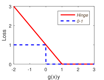
(a) Hinge loss

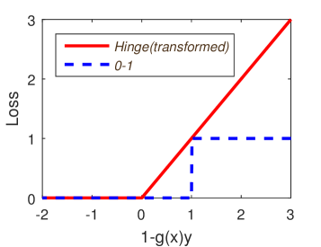
(b) Transfered hinge loss

Figure 1: Plot of the hinge loss function and a transferred plot with the mapping $1-g(x)y$.

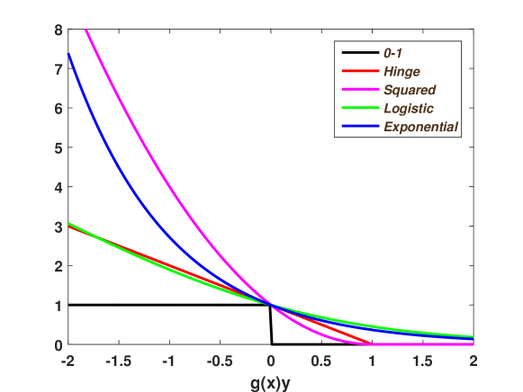
Figure 2: Some common convex surrogates for binary prediction as tight upper bounds on the 0-1 step loss (cf. [21, Figure 10.4].

In the sequel, we will use the notation for $l:\mathcal{P}(V)\mapsto\mathbb{R}$ as in Equation (9). Note that at the vertices, $\Delta(y,\cdot)$ has the following values:

$$l(\emptyset)\ \textrm{at}\ \mathbf{0}_{p}$$ (19)

$$l(\mathbf{I})\ \textrm{at}\ \{v|v\in\{0,1\}^{p},v^{i}=1\Leftrightarrow i\in\mathbf{I}\}$$ (20)

We call $l(\mathbf{I})$ the value of $l$ at the vertex $\mathbf{I}$.

We denote the operators for margin and slack rescaling that map the loss function to its convex surrogates $\mathbf{M}$ and $\mathbf{S}$, respectively. These operators have the same signature as $\mathbf{B}$ in Equation (4).

$$\mathbf{M}\Delta(y,g(x)):=\max_{\tilde{y}\in\mathcal{Y}}\Delta(y,\tilde{y})+\langle g(x),\tilde{y}\rangle-\langle g(x),y\rangle$$ (21)

$$\mathbf{S}\Delta(y,g(x)):=\max_{\tilde{y}\in\mathcal{Y}}\Delta(y,\tilde{y})\big{(}1+\langle g(x),\tilde{y}\rangle-\langle g(x),y\rangle\big{)}$$ (22)

respectively.

3.2 Slack rescaling

Proposition 1.

$\mathbf{S}\Delta(y,\cdot)$ is an extension of a set function $\Delta(y,\cdot)$ iff $\Delta(y,\cdot)$ is an increasing function.

Proof.

First we demonstrate the necessity. Given $\mathbf{S}\Delta(y,\cdot)$ an extension of $\Delta(y,\cdot)$, we analyse whether $\Delta(y,\cdot)$ is an increasing function.

As $\mathbf{S}\Delta(y,g(x))$ is an extension of $\Delta(y,\operatorname{sign}(g(x)))$, by Definition 3, $\mathbf{S}\Delta(y,g(x))=\Delta(y,\operatorname{sign}(g(x)))$ at the vertices as in (19) and (20):

First, at $u=\mathbf{0}$, while $u$ is defined as in Equation (18), we have $g^{j}(x)y^{j}=1$ then implies $g^{j}(x)\tilde{y}^{j}=1$ in our binary cases. By definition in Equation (22), $\mathbf{S}\Delta(y,g(x))=l(\emptyset)$ is always true for arbitrary (including increasing) $l$.

Second, at $u\in\mathbb{R}^{p}\setminus\{\mathbf{0}\}$, let $\mathbf{I}=\{i|u^{i}\neq 0\}$, then according to Equation (22),

$$\mathbf{S}\Delta(y,g(x)) =\max_{\mathbf{I}\in\mathcal{P}(V)}\ l(\mathbf{I})\big{(}1-2\sum_{i\in\mathbf{I}}g^{i}(x)y^{i}\big{)}$$ (23)

Let $\mathbf{I}_{2}=\arg\max_{\mathbf{I}\in\mathcal{P}(V)}l(\mathbf{I})\big{(}1-2\sum_{i\in\mathbf{I}}g^{i}(x)y^{i}\big{)}$. Given $\mathbf{S}\Delta(y,g(x))$ is an extension, we have

$$\mathbf{S}\Delta(y,g(x))=l(\mathbf{I}_{2})\big{(}1-2\sum_{i\in\mathbf{I}_{2}}g^{i}(x)y^{i}\big{)}=l(\mathbf{I}_{2}),$$

At the vertex $\mathbf{I}_{2}$, $\forall i\in\mathbf{I}_{2},u^{i}=1,g^{i}(x)y^{i}=0$. Meanwhile, as $\mathbf{I}_{2}$ is the maximizer of Equation (23), $\forall\mathbf{I}_{1}\in\mathcal{P}(V)\setminus\{\emptyset\}$,

$$l(\mathbf{I}_{2}) \geq l(\mathbf{I}_{1})\big{(}1-2\sum_{i\in\mathbf{I}_{1}}g^{i}(x)y^{i}\big{)},$$

$$=l(\mathbf{I}_{1})\big{(}1-2\sum_{i\in\mathbf{I}_{2}\cap\mathbf{I}_{1}}g^{i}(x)y^{i}-2\sum_{{\tiny i\in(V\setminus\mathbf{I}_{2})\cap\mathbf{I}_{1}}}g^{i}(x)y^{i}\big{)},$$

$$=l(\mathbf{I}_{1})\big{(}1-2|(V\setminus\mathbf{I}_{2})\cap\mathbf{I}_{1}|\big{)}.$$

The last line is due to the fact that at the vertex, $g^{i}(x)y^{i}=\{1,0\}^{p}$. Thus we have

$$\forall\mathbf{I}_{1}\in\mathcal{P}(V)\setminus\{\emptyset\},\ l(\mathbf{I}_{2})\geq l(\mathbf{I}_{1})\left(1-2|(V\setminus\mathbf{I}_{2})\cap\mathbf{I}_{1}|\right)$$ (24)

Given $\mathbf{S}\Delta(y,g(x))$ is an extension, $\mathbf{S}\Delta(y,g(x))=\Delta(y,\operatorname{sign}(g(x)))$ at the vertex $\mathbf{I}_{2}$. This leads also to two cases,

1. if $|(V\setminus\mathbf{I}_{2})\cap\mathbf{I}_{1}|=0$, $(V\setminus\mathbf{I}_{2})\cap\mathbf{I}_{1}=\emptyset$, which implies $\mathbf{I}_{1}\subseteq\mathbf{I}_{2}$, then from Equation (24) we get $l(\mathbf{I}_{2})\geq l(\mathbf{I}_{1})$. This implies that $l$ and therefore $\Delta$ are increasing;

2. if $|(V\setminus\mathbf{I}_{2})\cap\mathbf{I}_{1}|\geq 1$, this means the right-hand side of Equation (24) is negative, then it turns out to be redundant with $l(\mathbf{I}_{2})\geq 0$ which is always true.

To conclude, given $\mathbf{S}\Delta(y,\cdot)$ is an extension of a set function $\Delta(y,\cdot)$, it is always the case that $\Delta$ is increasing.

To demonstrate the sufficiency, we need to show that if $l$ is increasing, $\mathbf{S}\Delta(y,g(x))=\Delta(y,\operatorname{sign}(g(x)))$ at the vertices as in both (19) and (20):

First, at $u=\mathbf{0}$, through the similar analysis as before, we always have $u$ defined as in Equation (18) then $g^{j}(x)y^{j}=1$ and implies $g^{j}(x)\tilde{y}^{j}=1$ in our binary cases. By definition in Equation (22), $\mathbf{S}\Delta(y,g(x))=l(\emptyset)$ is always true.

Second, at $u\in\mathbb{R}^{p}\setminus\{\mathbf{0}\}$, denote one arbitrary vertex $\mathbf{I}\in\mathcal{P}(V)$, $u^{i}=1,i\in\mathbf{I}$,

$$l(\mathbf{I})\big{(}1-2\sum_{i\in\mathbf{I}}g^{i}(x)y^{i}\big{)}=l(\mathbf{I}).$$

Given $l$ is increasing, $\forall\mathbf{I}_{1}\subseteq\mathbf{I}$, we have $l(\mathbf{I}_{1})\leq l(\mathbf{I})$, and $u^{i}=1,i\in\mathbf{I}_{1}$, which leads to

$$l(\mathbf{I})\big{(}1-2\sum_{i\in\mathbf{I}}g^{i}(x)y^{i}\big{)} =l(\mathbf{I})$$

$$\geq l(\mathbf{I}_{1}) =l(\mathbf{I}_{1})\big{(}1-2\sum_{i\in\mathbf{I}_{1}}g^{i}(x)y^{i}\big{)}.$$

As this $\mathbf{I}$ can an arbitrary one, we can then fine the maximizer of Equation (23) $\mathbf{I}_{2}$ that $l(\mathbf{I}_{2})\big{(}1-2\sum_{i\in\mathbf{I}}g^{i}(x)y^{i}\big{)}=l(\mathbf{I}_{2})$ holds. This means $\mathbf{S}\Delta(y,\cdot)=l(\mathbf{I}_{2})$ at this vertex $\mathbb{I}_{2}$.

By conclusion, we proved that $\mathbf{S}\Delta(y,\cdot)$ yields a extension of $\Delta(y,\cdot)$ iff $\Delta(y,\cdot)$ is increasing. ∎

3.3 Margin rescaling

It is a necessary, but not sufficient condition that $\Delta(y,\tilde{y})$ be increasing for margin rescaling to yield an extension. However, we note that for all increasing $\Delta(y,\tilde{y})$ there exists a positive scaling $\gamma\in\mathbb{R}$ such that margin rescaling yields an extension. This is an important result for regularized risk minimization as we may simply rescale $\Delta$ to guarantee that margin rescaling yields an extension, and simultaneously scale the regularization parameter such that the relative contribution of the regularizer and loss is unchanged at the vertices of the unit cube.

Proposition 2.

For any loss function $\Delta$ corresponding to an increasing function $l\colon 2^{V}\to\mathbb{R}$ under the mapping in Equation (9), a positive factor $\gamma$ exists such that $\mathbf{M}\gamma\Delta(y,\cdot)$ yields an extension of $\gamma\Delta(y,\cdot)$. We denote $\mathbf{M}\gamma\Delta$ and $\gamma\Delta$ as the rescaled functions.

Proof.

Similar to Proposition 1, we analyse two cases to determine the values of $\mathbf{M}\gamma\Delta(y,g(x))$:

1. if $u=\mathbf{0},\ \mathbf{M}\gamma\Delta(y,g(x))=\gamma l(\emptyset)$ where $u$ is defined as in Equation (18). It is typically the case that $l(\emptyset)=0$, but this is not a technical requirement.

2. if $u\neq\mathbf{0}$, let $\mathbf{I}=\{i|u^{i}\neq 0\}$, then $\mathbf{M}\gamma\Delta(y,g(x))$ takes the value of the following equation:

   $$\max_{\mathbf{I}\in\mathcal{P}(V)}\ \gamma l(\mathbf{I})-2\sum_{i\in\mathbf{I}}g^{i}(x)y^{i}$$ (25)

To satisfy Definition 3, we must find a $\gamma>0$ such that $\mathbf{M}\gamma\Delta(y,g(x))=\gamma\Delta(y,\operatorname{sign}(g(x)))$ at the vertices. Note that it is trivial when $u=\mathbf{0}$ so the first case is true for arbitrary $\gamma>0$.

For the second case, let $\mathbf{I}_{2}=\arg\max_{\mathbf{I}\in\mathcal{P}(V)}\big{(}\gamma l(\mathbf{I})-\sum_{i\in\mathbf{I}}g^{i}(x)y^{i}\big{)}$. Given $\mathbf{M}\gamma\Delta(y,g(x))$ is an extension, we have $\mathbf{M}\gamma\Delta(y,g(x))=\gamma\Delta(y,\operatorname{sign}(g(x)))$ at the vertices $\mathbf{I}_{2}$, that is:

$$\mathbf{M}\gamma\Delta(y,g(x)) =\gamma l(\mathbf{I}_{2})-2\sum_{i\in\mathbf{I}_{2}}g^{i}(x)y^{i}=\gamma l(\mathbf{I}_{2}).$$

Meanwhile, as $\mathbf{I}_{2}$ is the maximizer of Equation (25), we also have

$$\mathbf{M}\gamma\Delta(y,g(x)) =\gamma l(\mathbf{I}_{2})$$

$$\geq\gamma l(\mathbf{I}_{1})-2\sum_{i\in\mathbf{I}_{1}}g^{i}(x)y^{i},\ \forall\mathbf{I}_{1}\in\mathcal{P}(V)\setminus\{\emptyset\},$$

which implies that the scale factor should satisfy:

$$\gamma\left(l(\mathbf{I}_{2})-l(\mathbf{I}_{1})\right) \geq-2\sum_{i\in\mathbf{I}_{1}}g^{i}(x)y^{i}$$

$$\geq-2\sum_{i\in\mathbf{I}_{2}\cap\mathbf{I}_{1}}g^{i}(x)y^{i}-2\sum_{i\in(V\setminus\mathbf{I}_{2})\cap\mathbf{I}_{1}}g^{i}(x)y^{i}$$

$$\geq-2|(V\setminus\mathbf{I}_{2})\cap\mathbf{I}_{1}|$$ (26)

This leads to the following cases:

1. if $|(V\setminus\mathbf{I}_{2})\cap\mathbf{I}_{1}|=0$, we have $(V\setminus\mathbf{I}_{2})\cap\mathbf{I}_{1}=\emptyset$, which implies $\mathbf{I}_{1}\subseteq\mathbf{I}_{2}$. Equation (26) reduces to

   $$\gamma\big{(}l(\mathbf{I}_{2})-l(\mathbf{I}_{1})\big{)}\geq 0$$ (27)

   and $l$ is an increasing function so $l(\mathbf{I}_{1})\leq l(\mathbf{I}_{2})$, then Equation (27) is always true as $\gamma>0$.

2. if $|(V\setminus\mathbf{I}_{2})\cap\mathbf{I}_{1}|\neq 0$, we need to discuss between $l(\mathbf{I}_{1})$ and $l(\mathbf{I}_{2})$:

   1. if $l(\mathbf{I}_{2})=l(\mathbf{I}_{1})$, then Equation (27) becomes $0\geq-|(V\setminus\mathbf{I}_{2})\cap\mathbf{I}_{1}|$, for which the right-hand side is negative so it is always true.

   2. if $l(\mathbf{I}_{2})>l(\mathbf{I}_{1})$, then

      $$\gamma\geq\frac{-2|(V\setminus\mathbf{I}_{2})\cap\mathbf{I}_{1}|}{l(\mathbf{I}_{2})-l(\mathbf{I}_{1})}$$ (28)

      for which the right-hand side is negative so it is redundant with $\gamma>0$ .

   3. if $l(\mathbf{I}_{2})<l(\mathbf{I}_{1})$, then

      $$\gamma\leq\frac{-2|(V\setminus\mathbf{I}_{2})\cap\mathbf{I}_{1}|}{l(\mathbf{I}_{2})-l(\mathbf{I}_{1})}$$ (29)

      for which the right-hand side is strictly positive so it becomes an upper bound on $\gamma$ .

In summary the scale factor $\gamma$ should satisfy the following constraint for an increasing loss function $l$:

$$\forall\mathbf{I}_{1},\mathbf{I}_{2}\in\mathcal{P}(V)\setminus\{\emptyset\},0<\gamma\leq\frac{-2|(V\setminus\mathbf{I}_{2})\cap\mathbf{I}_{1}|}{l(\mathbf{I}_{2})-l(\mathbf{I}_{1})}$$

Finally, we note that the rightmost ratio is always strictly positive. ∎

3.4 Complexity of subgradient computation

Although we have proven that slack and margin rescaling yield extensions to the underlying discrete loss under fairly general conditions, their key shortcoming is in the complexity of the computation of subgradients for submodular losses. The subgradient computation for slack and margin rescaling requires the computation of

$$\arg\max_{\tilde{y}}\Delta(y,\tilde{y})(1+h(x,\tilde{y})-h(x,y))$$ (30)

and

$$\arg\max_{\tilde{y}}\Delta(y,\tilde{y})+h(x,\tilde{y}),$$ (31)

respectively. For both margin and slack rescaling, a submodular function must be maximized as shown above, given that $\Delta$ is submodular. This computation is NP-hard, and such loss functions are not feasible with these existing methods in practice. Furthermore, approximate inference, e.g. based on [22], leads to poor convergence when used to train a structured output SVM resulting in a high error rate (cf. Section 6, Tables I-IV). We therefore introduce the Lovász hinge as an alternative operator to construct feasible convex surrogates for submodular losses.

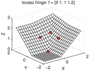
(a) Lovász hinge with submodular increasing $l$

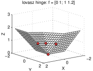
(b) Lovász hinge with submodular increasing $l$

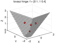
(c) Lovász hinge with submodular non-monotonic $l$

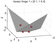
(d) Lovász hinge with submodular non-monotonic $l$

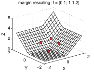
(e) Margin-rescaling with submodular increasing $l$

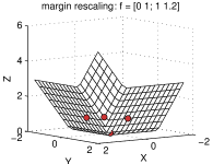
(f) Margin-rescaling with submodular increasing $l$

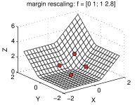
(g) Margin-rescaling with supermodular increasing $l$

(h) Margin-rescaling with supermodular increasing $l$

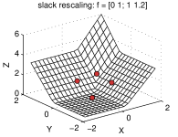
(i) Slack-rescaling with submodular increasing $l$

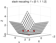
(j) Slack-rescaling with submodular increasing $l$

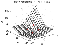
(k) Slack-rescaling with supermodular increasing $l$

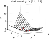
(l) Slack-rescaling with supermodular increasing $l$

Figure 3: We introduce a novel convex surrogate for submodular losses, the Lovász hinge. We show here the Lovász hinge, margin and slack rescaling surfaces with different loss functions $l$ from different views; the $x$ and $y$ axes represent the value of $s_{i}^{1}$ and $s_{i}^{2}$ in Eq. (34); the $z$ axis represents the value of the convex surrogate; the solid red dots represent the values of $l$ at the vertices of the unit hypercube. The convex surrogate strategies yield extensions of the discrete loss.

4 Lovász Hinge

We now develop our convex surrogate for submodular loss functions, which is based on the Lovász extension. In the sequel, the notion of permutations is important. We denote a permutation of $p$ elements by $\pi=(\pi_{1},\pi_{2},\dots,\pi_{p})$, where $\pi_{i}\in\{1,2,\dots p\}$ and $\pi_{i}\neq\pi_{j},\ \forall i\neq j$. Furthermore, for a vector $s\in\mathbb{R}^{p}$, we will be interested in the permutation $\pi$ that sorts the elements of $s$ in decreasing order, i.e. $s^{\pi_{1}}\geq s^{\pi_{2}}\geq\dots\geq s^{\pi_{p}}$. Without loss of generality, we will index the base set of a set function $l$ by integer values, i.e. $V=\{1,2,\dots,p\}$, so that for a permutation $\pi$, $l(\{\pi_{1},\pi_{2},\dots,\pi_{i}\})$ is well defined.

4.1 Lovász extension

In this section, we introduce a novel convex surrogate for submodular losses. This surrogate is based on a fundamental result relating submodular set functions and piecewise linear convex functions, called the Lovász extension [23]. It allows the extension of a set function defined on the vertices of the hypercube $\{0,1\}^{p}$ to the full hypercube $[0,1]^{p}$:

Definition 4 (Lovász extension [23]).

Consider a set function $l:\mathcal{P}(V)\mapsto\mathbb{R}$ where $|V|=p$. The Lovász extension $\hat{l}:[0,1]^{p}\to\mathbb{R}$ of $l$ is defined as follows: $\forall s\in[0,1]^{p}$ we order its components in decreasing order as $s^{\pi_{1}}\geq s^{\pi_{2}}\geq\cdots\geq s^{\pi_{p}}$ with a permutation $\pi$, then $\hat{l}(s)$ is defined as:

$$\hat{l}(s)=\sum_{j=1}^{p}s^{\pi_{j}}\left(l\left(\{\pi_{1},\cdots,\pi_{j}\}\right)-l\left(\{\pi_{1},\cdots,\pi_{j-1}\}\right)\right).$$ (32)

Associated with a submbodular function there are two polyhedra are commonly introduced:

Definition 5.

For a submodular function $l$, we call $P(l)=\{s\in\mathbb{R}^{p}|$ $\forall A\subseteq V$, $\sum_{i\in A}s^{i}\leq l(A)\}$ the submodular polyhedron, and $B(l)=P(l)\cap\{s\in\mathbb{R}^{p}|\sum_{i\in V}s^{i}=l(V)\}$ the base polyhedron.

The Lovász extension connects submodular set functions and convex functions. Furthermore, we may substitute convex optimization of the Lovász extension for discrete optimization of a submodular set function:

Proposition 3 (Greedy algorithm [23, 24]).

We have a submodular function $l$ such that $l(\emptyset)=0$, $\forall s\in[0,1]^{p}$ we order its components in decreasing order as in Definition 4 with a permutation $\pi$. We denote $\mu^{\pi_{j}}=l\left(\{\pi_{1},\cdots,\pi_{j}\}\right)-l\left(\{\pi_{1},\cdots,\pi_{j-1}\}\right)$, then $\mu$ is on the base polyhedron i.e. $\mu\in B(l)$, and

1. if $s\in\mathbb{R}^{p}_{+}$, $\mu$ is a maximizer of $\max_{\mu\in B(l)}s^{\intercal}\mu$, and $\max_{\mu\in B(l)}s^{\intercal}\mu=\hat{l}(s)$;

2. $\mu$ is a maximizer of $\max_{\mu\in P(l)}s^{\intercal}\mu$, and $\max_{\mu\in P(l)}s^{\intercal}\mu=\hat{l}(s)$;

A proof with detailed analysis can be found in [25, Proposition 3.2 to 3.5]. That is to say, to find a maximum of $s^{\intercal}\mu$, which is the same procedure as computing a subgradient of the Lovász extension, is precisely the following procedure:

1. sort the $p$ components of $s$, which is in $\mathcal{O}(p\log p)$;

2. compute the value of $s^{\intercal}\mu$ which needs $\mathcal{O}(p)$ oracle accesses to the set function.

Proposition 4 (Equivalence between the greedy algorithm and maximization over permutations).

The Lovász extension can equivalently be written:

$$\hat{l}(s)=\max_{\pi}\sum_{j=1}^{p}s^{\pi_{j}}\left(l\left(\{\pi_{1},\cdots,\pi_{j}\}\right)-l\left(\{\pi_{1},\cdots,\pi_{j-1}\}\right)\right).$$ (33)

Proof.

From [26, Equation (4)] we have that every permutation characterizes an extremal point of the submodular polyhedron. From Proposition 3 we have that the Lovász extension is an LP over this polyhedron and one of the extremal points must therefore be a solution [27, Theorem 22]. ∎

Proposition 5 (Convexity and submodularity [23]).

A function $l$ is submodular if and only if its Lovász extension $\hat{l}$ is convex.

A proof of this proposition is given in [25, Proposition 3.6]. We then take the advantage of this proposition to define a novel convex surrogate for submodular loss functions.

4.2 Lovász hinge

We propose our novel convex surrogate for submodular functions in Definition 6.

Definition 6.

For $l$ submodular, the Lovász hinge $\mathbf{L}$ is defined as the unique operator such that,

$$\mathbf{L}\Delta(y,g(x)):=\max_{\pi}$$

$$\begin{cases}&\sum_{j=1}^{p}\left(s^{\pi_{j}}\right)_{+}\left(l\left(\{\pi_{1},\cdots,\pi_{j}\}\right)-l\left(\{\pi_{1},\cdots,\pi_{j-1}\}\right)\right)\\ &\qquad 1.\ \text{ if $l$ increasing}\\ &\left(\sum_{j=1}^{p}s^{\pi_{j}}\left(l\left(\{\pi_{1},\cdots,\pi_{j}\}\right)-l\left(\{\pi_{1},\cdots,\pi_{j-1}\}\right)\right)\right)_{+}\\ &\qquad 2.\ \text{otherwise}\\ \end{cases}$$

where $(\cdot)_{+}=\max(\cdot,0)$, $\pi$ is a permutation,

$$s^{\pi_{j}}=1-g^{\pi_{j}}(x)y^{\pi_{j}},$$ (34)

and $g^{\pi_{j}}(x)$ is the $\pi_{j}$th coordinate of $g(x)$ (cf. Equation (16)).

Note that the Lovász hinge is itself an extension of the Lovász extension (defined over the $p$-dimensional unit cube) to $\mathbb{R}^{p}$. For $l$ being submodular increasing, we threshold each negative component of $s$ i.e. $s^{\pi_{j}}=1-g^{\pi_{j}}(x)y^{\pi_{j}}$ to zero. As $l$ being increasing, the components $l\left(\{\pi_{1},\cdots,\pi_{j}\}\right)-l\left(\{\pi_{1},\cdots,\pi_{j-1}\}\right)$ will always be non-negative. Then $\mathbf{L}\Delta(y,g(x))$ in Definition 6 case 1 is always non-negative. While in Definition 6 case 2, we don’t apply the thresholding strategy on the components of $s$, but instead on the entire formulation.

We show in the following propositions that these two definitions yield surrogates that are indeed convex and extensions of the corresponding loss functions.

Proposition 6.

For a submodular non-negative loss function $l$, the Lovász hinge as in Definition 6 case 2 is convex and yields an extension of $\Delta$.

Proof.

We first demonstrate the “convex” part. It is clear that taking a maximum over linear functions is convex. The thresholding to non-negative values similarly maintains convexity.

We then demonstrate the “extension” part. From the definition of extension as in Equation (18) as well as the notation concerning the vertices of the unit cube as in Equation (20), for the values of $s$ on the vertices $\mathbf{I}$, we have explicitly

$$s^{j}=\left\{\begin{array}[]{ll}1,&\ \forall j\in\mathbf{I}\\ 0,&\ \forall j\in V\setminus\mathbf{I}\end{array}\right.$$ (35)

As a result, the permutation $\pi$ that sorts the components of $s$ decreasing on the vertices is actually

$$\{\pi_{1},\cdots,\pi_{k},\pi_{k+1},\cdots,\pi_{p}\},\ k=|\mathbf{I}|.$$

with $\{\pi_{1},\cdots,\pi_{k}\}$ a permutation of $\{j|j\in\mathbf{I}\}$, $s^{\pi_{1}}=\cdots=s^{\pi_{k}}=1$, and $\{\pi_{k+1},\cdots,\pi_{p}\}$ a permutation of $\{j|j\in V\setminus\mathbf{I}\}$, $s^{\pi_{k+1}}=\cdots=s^{\pi_{p}}=0$.

We then reformulate the inside part of the right-hand side of Definition 6 case 2 as:

$$\sum_{j=1}^{p}s^{\pi_{j}}\left(l\left(\{\pi_{1},\cdots,\pi_{j}\}\right)-l\left(\{\pi_{1},\cdots,\pi_{j-1}\}\right)\right)$$

$$=\sum_{j=1}^{k}1\times\left(l\left(\{\pi_{1},\cdots,\pi_{j}\}\right)-l\left(\{\pi_{1},\cdots,\pi_{j-1}\}\right)\right)+0$$

$$=l\left(\{\pi_{1},\cdots,\pi_{k}\}\right)$$

$$=l(\mathbf{I})$$ (36)

Then for non-negative $l$, thresholding is redundant. As a consequence we have

$$\mathbf{L}\Delta(y,g(x))=\left(l(\mathbf{I})\right)_{+}=\Delta(y,g(x))$$ (37)

which validates that $\mathbf{L}\Delta(y,g(x))$ yields an extension of $\Delta(y,g(x))$. ∎

Proposition 7.

For a submodular increasing loss function $l$ , the Lovász hinge as in Definition 6 case 1 is convex and yields an extension of $\Delta$.

Proof.

We first demonstrate the “convex” part. When $l$ is increasing, $\mu^{\pi_{j}}=l\left(\{\pi_{1},\cdots,\pi_{j}\}\right)-l\left(\{\pi_{1},\cdots,\pi_{j-1}\}\right)$ will always be positive for all $\pi_{j}\in\{1,2,\cdots,p\}$. So it’s obvious that $\mu^{\pi_{j}}\times\max(0,s^{\pi_{j}})$ will always be convex with respect to $s^{\pi_{j}}\in\mathbb{R}$ for any given $\mu^{\pi_{j}}\geq 0$. As the convex function set is closed under the operation of addition, the Lovász hinge is convex in $\mathbb{R}^{p}$.

We note that on the vertex $\mathbf{I}$, we have $s\in\{0,1\}^{p}$ as in Equation (35), then the positive threshold on the components of $s^{j}$ can be removed. With the same procedure as in Equation (36), $\mathbf{L}\Delta(y,g(x))$ yields an extension of $\Delta(y,g(x))$. ∎

Although Definition 6 case 1 and case 2 is convex and yields an extension for both increasing and non-monotonic losses, we rather apply Definition 6 case 1 for increasing loss functions. This will ensure the Lovász hinge is an analogue to a standard hinge loss in the special case of a symmetric modular loss. We formally state this as the following proposition:

Proposition 8.

For a submodular increasing loss function $l$, the Lovász hinge as in Definition 6 case 1 thresholding negative $s^{\pi_{j}}$ to zero, coincides with an SVM (i.e. additive hinge loss) in the case of Hamming loss.

Proof.

The hinge loss for a set of $p$ training samples is defined to be

$$\ell_{\text{hinge}}(y,g(x)):=\sum_{i=1}^{p}\left(1-g(x^{i})y^{i})\right)_{+}.$$ (38)

Following the previous notation, we will interpret $g(x^{i})=g^{i}(x)$. For a modular loss, the Lovász hinge in Definition 6 case 1 simplifies to

$$\mathbf{L}\Delta(y,g(x)) = \max_{\pi}\sum_{j=1}^{p}(s^{\pi_{j}})_{+}l(\{\pi_{j}\})$$ (39)

$$= \sum_{j=1}^{p}\left(1-g^{j}(x)y^{j}\right)_{+}l(\{j\}).$$ (40)

For the Hamming loss $l(\{j\})=1,\forall j$ and $\mathbf{L}\Delta(y,g(x))=\ell_{\text{hinge}}(y,g(x))$. ∎

Lemma 1.

The convex closure of a set function $l$ is the largest function $l_{\text{c}}:[0,1]^{p}\mapsto\mathbb{R}\cup\{+\infty\}$ such that (a) $l_{\text{c}}$ is convex and (b) for all $A\subseteq V,l_{\text{c}}(1_{A})\leq l(A)$, where $1_{A}$ is a binary vector such that the $i$th element is one iff $i\in A$ and zero otherwise. The Lovász extension of a submodular function $l$ coincides with its convex closure [25, 28].

Proposition 9.

The Lovász hinge has an equal or higher value than slack and margin rescaling inside the unit cube.

Proof.

Inside the unit cube $s\in[0,1]^{p}$, $(s^{i})=s^{i}$ for all $i$ and the Lovász hinge coincides with the Lovász extension. Then by Lemma 1 we have that the Lovász hinge inside the unit cube is the maximum convex extension, and therefore slack and margin rescaling must have equal or lesser values. ∎

Corollary 1.

Slack and margin rescaling may have additional inflection points inside the unit cube that are not present in the Lovász hinge. This is a consequence of Proposition 9 and the fact that all three are piecewise linear extensions, and thus have identical values on the vertices of the unit cube. One can also visualize this in Figure 3.

Another reason that we use a different threshold strategy on $s$ for increasing or non-monotonic losses is that we cannot guarantee that the Lovász hinge is always convex if we threshold each negative component $s^{\pi_{j}}$ to zero for non-monotonic losses.

Proposition 10.

For a submodular non-monotonic loss function $l$ , the Lovász hinge is not convex if we threshold each negative component $s^{\pi_{j}}$ to zero as in Definition 6 case 1.

Proof.

If $l$ is non-monotonic, there exists at least one $\pi$ and $j$ such that $\mu^{\pi_{j}}:=l\left(\{\pi_{1},\cdots,\pi_{j}\}\right)-l\left(\{\pi_{1},\cdots,\pi_{j-1}\}\right)$ is strictly negative. The partial derivative of $\mathbf{L}\Delta(y,g(x))$ w.r.t. $s^{\pi_{j}}$ is

$$\frac{\partial\mathbf{L}\Delta(y,g(x))}{\partial s^{\pi_{j}}}=\begin{cases}0&\text{if }s^{\pi_{j}}<0\\ \mu^{\pi_{j}}&\text{if }s^{\pi_{j}}>0.\end{cases}$$ (41)

As $\mu^{\pi_{j}}<0$ by assumption, we have that the partial derivative at $s^{\pi_{j}}<0$ is larger than the partial derivative at $s^{\pi_{j}}>0$, and the loss surface cannot therefore be convex. ∎

Figure 4 and Figure 4 show an example of the loss surface when $l$ is non-monotonic. We can see that the decreasing element leads to a negative subgradient at one side of a vertex, while on its other side the subgradient is zero due to the fact that we still apply the thresholding strategy. Thus it leads to a non-convex surface.

4.3 Complexity of subgradient computation

We explicitly present the cutting plane algorithm for solving the max-margin problem as in Equation (12) in Algorithm 2. The novelties are: (i) in Line 5 we calculate the upper bound on the empirical loss by the Lovász hinge; (ii) in Line 6 we calculate the loss gradient by the computation relating to the permutation $\pi$ instead of to all possible outputs $\tilde{y}$.

Algorithm 2 Cutting plane algorithm for solving the problem in Equation (12), with Definition 6 – the Lovász hinge.

1:  Input: $(x_{1},y_{1}),\cdots,(x_{n},y_{n}),C,\epsilon$

2:  $S^{i}=\emptyset,\forall i=1,\cdots,n$

3:  repeat

4:     for $i=1,\cdots,n$ do

5:        

$H(y_{i},\pi)=\sum_{j=1}^{p}s_{i}^{\pi_{j}}\left(l\left(\{\pi_{1},\cdots,\pi_{j}\}\right)-l\left(\{\pi_{1},\cdots,\pi_{j-1}\}\right)\right)$

, where $s^{\pi_{j}}=1-g^{\pi_{j}}(x_{i})y_{i}^{\pi_{j}}$

6:         $\hat{\pi}=\arg\max_{\pi}H(y_{i},\pi)$ % find the most violated constraint by sorting the $p$ elements of $s$

7:        $\xi^{i}=\max\{0,H(y_{i},\hat{\pi})\}$

8:        if $H(y_{i},\hat{\pi})>\xi^{i}+\epsilon$  then

9:           $S^{i}:=S^{i}\cup\{\hat{\pi}\}$

10:           $w\leftarrow$ optimize Equation (12) with constraints defined by $\cup_{i}S^{i}$

11:        end if

12:     end for

13:  until no $S^{i}$ has changed during iteration

14:  return  $(w,\xi)$

As the computation of a cutting plane or loss gradient is precisely the same procedure as computing a value of the Lovász extension, we have the same computational complexity, which is $\mathcal{O}(p\log p)$ to sort the $p$ coefficients, followed by $\mathcal{O}(p)$ oracle accesses to the loss function [23]. This is precisely an application of the greedy algorithm to optimize a linear program over the submodular polytope as shown in Proposition 3. In our implementation, we have employed a one-slack cutting-plane optimization with $\ell_{2}$ regularization analogous to [29]. We observe empirical convergence of the primal-dual gap at a rate comparable to that of a structured output SVM (Fig. 8).

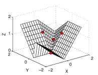
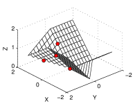
Figure 4: Lovász hinge with submodular non-monotonic $l$ while thresholding negative components of $s$ is still applied (cf. the caption of Figure 3 for the axes notation). Although the red dots touch the surface, the surface is no longer convex due to the thresholding strategy.

4.4 Visualization of convex surrogates

For visualization of the loss surfaces, in this section we consider a simple binary classification problem with two elements with non-modular loss functions :

$$\mathcal{X}:=\mathbb{R}^{d\times 2}\qquad\mathcal{Y}:=\{-1,+1\}^{2}$$

Then with different values for $l(\emptyset)$, $l(\{1\})$, $l(\{2\})$ and $l(\{1,2\})$, we can have different modularity or monotonicity properties of the function $l$ which then defines $\Delta$. We illustrate the Lovász hinge, slack and margin rescaling for the following cases:

1. submodular increasing:
   $l(\emptyset)=0,\ l(\{1\})=l(\{2\})=1,\ l(\{1,2\})=1.2$,

2. submodular non-monotonic:
   $l(\emptyset)=0,\ l(\{1\})=l(\{2\})=1,\ l(\{1,2\})=0.4$, and

3. supermodular increasing:
   $l(\emptyset)=0,\ l(\{1\})=l(\{2\})=1,\ l(\{1,2\})=2.8$.

In Fig. 3, the $x$ axis represents the value of $s^{1}$, the $y$ axis represents the value of $s^{2}$ in Eq (34), and the $z$ axis is the convex loss function given by Equation (21), Equation (22), and Definition 6 for different loss functions. We plot the values of $l$ as solid dots at the vertices of the hypercube.

We observe first that all surfaces are convex. For the Lovász hinge with a submodular increasing function in Figure 3(a) and Figure 3(b), the thresholding strategy adds two hyperplanes on the left and on the right, while convexity is maintained. We observe then that all the solid dots corresponding to the discrete loss fuction values touch the surfaces, which empirically validates that the surrogates are extensions of the discrete loss. Here we set $l$ as symmetric functions, while the extensions can be also validated for asymmetric increasing set functions.

We additionally plot the Lovász hinge with a non-monotonic function while the thresholding strategy on $s$ is still applied in Figure 4. Compared to Figure 3(c) and Figure 3(d), convexity is lost due to the thresholding strategy on negative components of $s$.

5 Jaccard Loss

The Jaccard index score is a popular measure for comparing the similarity between two sample sets, widely applied in diverse prediction problems such as structured output prediction [6], social network prediction [30] and image segmentation [31]. It is used in the evaluation of popular computer vision challenges, such as PASCAL VOC [32] and ImageNet [33, Sec. 4.2]. In this section, we introduce the Jaccard loss based on the Jaccard index score, and we prove that the Jaccard loss is a submodular function with respect to the set of mispredicted elements.

We will use $P_{y},P_{\tilde{y}}\subseteq V$ to denote sets of positive predictions. We define the Jaccard loss to be [6]

$$\Delta_{J}(y,\tilde{y}):=1-\frac{|P_{y}\cap P_{\tilde{y}}|}{|P_{y}\cup P_{\tilde{y}}|}$$ (42)

We now show that this is submodular under the isomorphism $(y,\tilde{y})\rightarrow A:=\{i|y_{i}\neq\tilde{y}_{i}\}$, $\Delta_{J}(y,\tilde{y})\cong l(A)$. We will use the diminishing returns definition of submodularity as in Definition 1. We will denote $m:=|P_{y}|>0$, $p:=|P_{\tilde{y}}\setminus P_{y}|$, and $n:=|P_{y}\setminus P_{\tilde{y}}|$. With this notation, we have that

$$\Delta_{J}(y,\tilde{y})=1-\frac{m-n}{m+p}$$ (43)

For a fixed groundtruth $y$, we have for two sets of mispredictions $A$ and $B$

$$\text{if }B\subseteq A\text{, then }\ n_{B}\leq n_{A},\ p_{B}\leq p_{A}$$ (44)

We first prove two lemmas about the submodularity of the loss function restricted to additional false positives or false negatives.

Lemma 2.

$\Delta_{J}$ restricted to marginal false negatives is submodular.

Proof.

If $i$ is an extra false negative,

$$\Delta_{J}(A\cup\{i\}) =\Delta_{J}(n_{A}+1,p_{A})$$

$$=\frac{n_{A}+p_{A}+1}{m+p_{A}}$$

$$=\Delta_{J}(A)+\frac{1}{m+p_{A}}$$ (45)

Then we have

$$\Delta_{J}(A\cup\{i\})-\Delta_{J}(A) =\frac{1}{m+p_{A}}$$

$$\leq\frac{1}{m+p_{B}}$$

$$=\Delta_{J}(B\cup\{i\})-\Delta_{J}(B)$$ (46)

which complies with the definition of submodularity. ∎

Lemma 3.

$\Delta_{J}$ restricted to marginal false positives is submodular.

Proof.

If $i$ is an extra false positive, with the similar procedure as previous, we have

$$\Delta_{J}(A\cup\{i\}) =\Delta_{J}(n_{A},p_{A}+1)$$

$$=\frac{n_{A}+p_{A}+1}{m+p_{A}+1}$$ (47)

$$\Delta_{J}(A\cup\{i\})-\Delta_{J}(A) =\frac{n_{A}+p_{A}+1}{m+p_{A}+1}-\frac{n_{A}+p_{A}}{m+p_{A}}$$

$$=\frac{|A|-n_{A}}{(m+p_{A}+1)(m+p_{A})}$$

$$\leq\frac{|A|-n_{B}}{(m+p_{B}+1)(m+p_{B})}$$

$$=\Delta_{J}(B\cup\{i\})-\Delta_{J}(B)$$ (48)

which also complies with the definition of submodularity. ∎

Proposition 11.

$\Delta_{J}$ is submodular.

Proof.

Lemmas 2 and 3 cover mutually exclusive cases whose union covers all possible marginal mistakes. As the diminishing returns property of submodularity (Equation (7)) holds in both cases, it also holds for the union. ∎

6 Experimental Results

We validate the Lovász hinge on a number of different experimental settings. In Section 6.1, we demonstrate a synthetic problem motivated by an early detection task. Next, we show that the Lovász hinge can be employed to improve image classification measured by the Jaccard loss on the PASCAL VOC dataset in Section 6.2. Multi-label prediction with submodular losses is demonstrated on the PASCAL VOC dataset in Section 6.3, and on the MS COCO dataset in Section 6.4. A summary of results is given in Section 6.5.

6.1 A Synthetic Problem

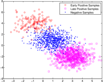
Figure 5: The disributions of samples for a synthetic binary classification problem motivated by the problem of early detection in a temporal sequence. As in, e.g. disease evolution, the distribution of early stage samples differs from that of late stage samples.

We designed a synthetic problem motivated by early detection in a sequence of observations. As shown in Fig. 5, each star represents one sample in a bag and $p=15$ samples form one bag. In each bag, the samples are arranged in a chronological order, with samples appearing earlier drawn from a different distribution than later samples. The red and magenta dots represent the early and late positive samples, respectively. The blue dots represent the negative samples. For the negative samples, there is no change in distribution between early and late samples, while the distribution of positive samples changes with time (e.g. as in the evolution of cancer from early to late stage).

We define the loss function as

$$\Delta_{1}(y,\tilde{y})=\sum_{i=1}^{p}\gamma_{i}l_{sub}(\mathbf{I}_{i})$$ (49)

where $\mathbf{I}_{i}=\{j|j\leq i,\tilde{y}^{j}\neq y^{j}\}$. Let $\gamma_{i}:=e^{-i}\ \forall i$. By this formulation, we penalize early mispredictions more than late mispredictions. This is a realistic setting in many situations where, e.g. early detection of a disease leads to better patient outcomes. The loss $l_{sub}$ measures the misprediction rate up to the current time while being limited by an upper bound:

$$l_{sub}(\mathbf{I}_{i}):=\min\left(|\mathbf{I}_{i}|,\ \frac{i}{2}\right).$$ (50)

As $\Delta$ is a positively weighted sum of submodular losses, it is submodular. We additionally train and test with the 0-1 loss, which is equivalent to an SVM and Hamming loss in the Lovász hinge. We use different losses during training and during testing, then we measure the empirical loss values of one prediction as the average loss value for all images shown in Table. I. We have trained on 1000 bags and tested on 5000 bags. $\mathbf{M}$ and $\mathbf{S}$ denote the use of the submodular loss with margin and slack rescaling, respectively. As this optimization is intractable, we have employed the approximate optimization procedure of [22].

As predicted by theory, training with the same loss function as used during testing yields the best results. Slack and margin rescaling fail due to the necessity of approximate inference, which results in a poor discriminant function. By contrast, the Lovász hinge yields the best performance on the submodular loss.

TABLE I: For the synthetic problem, the cross comparison of average loss values (with standard error) using different convex surrogates for the submodular loss in Equation (49) during training, 0-1 loss for comparison, and testing with different losses.

		Test
		$\Delta_{1}$	0-1
Train	$\mathbf{L}$	$\mathbf{0.100\pm 0.001}$	$7.42\pm 0.01$
	0-1	$0.166\pm 0.001$	$\mathbf{2.87\pm 0.02}$
	$\mathbf{S}$	$0.144\pm 0.001$	$7.69\pm 0.01$
	$\mathbf{M}$	$0.154\pm 0.001$	$3.01\pm 0.01$

6.2 PASCAL VOC image classification

We consider an image classification task on the Pascal VOC dataset [32]. This challenging dataset contains around 10,000 images of 20 classes including animals, handmade and natural objects such as person, bird, aeroplane, etc. In the training set, which contains 5,011 images of different categories, the number of positive samples varies largely, we evaluate the prediction on the entire training/testing set with the Jaccard loss as in Equation (42).

We use Overfeat [34] to extract image features following the procedure described in [35]. Overfeat has been trained for the image classification task on ImageNet ILSVRC 2013, and has achieved good performance on a range of image classification problems.

We compare learning with the Jaccard loss with the Lovász hinge with learning an SVM (labeled 0-1 in the results tables). The empirical error values using different loss function during test time are shown in Table II.

TABLE II: For the VOC image classification task, the cross comparison of average loss values using the Jaccard loss as well as 0-1 loss during training and during testing for the 20 categories.

		aeroplane		bicycle		bird		boat		bottle		bus		car		cat		chair		cow
Test time		$\Delta_{J}$	0-1	$\Delta_{J}$	0-1	$\Delta_{J}$	0-1	$\Delta_{J}$	0-1	$\Delta_{J}$	0-1	$\Delta_{J}$	0-1	$\Delta_{J}$	0-1	$\Delta_{J}$	0-1	$\Delta_{J}$	0-1	$\Delta_{J}$	0-1
Train	$\mathbf{L}$	$0.310$	$0.014$	$0.436$	$0.025$	$0.371$	$0.025$	$0.416$	$0.017$	$0.761$	$0.062$	$0.539$	$0.026$	$0.399$	$0.076$	$0.426$	$0.035$	$0.687$	$0.121$	$0.640$	$0.027$
	0-1	$0.310$	$0.014$	$0.466$	$0.027$	$0.399$	$0.025$	$0.483$	$0.020$	$0.917$	$0.045$	$0.661$	$0.025$	$0.397$	$0.068$	$0.469$	$0.034$	$0.744$	$0.090$	$0.892$	$0.023$
		diningtable		dog		horse		motorbike		person		pottedplant		sheep		sofa		train		tvmonitor
Test time		$\Delta_{J}$	0-1	$\Delta_{J}$	0-1	$\Delta_{J}$	0-1	$\Delta_{J}$	0-1	$\Delta_{J}$	0-1	$\Delta_{J}$	0-1	$\Delta_{J}$	0-1	$\Delta_{J}$	0-1	$\Delta_{J}$	0-1	$\Delta_{J}$	0-1
Train	$\mathbf{L}$	$0.664$	$0.055$	$0.475$	$0.054$	$0.405$	$0.029$	$0.439$	$0.025$	$0.347$	$0.180$	$0.747$	$0.058$	$0.580$	$0.017$	$0.710$	$0.062$	$0.306$	$0.018$	$0.588$	$0.042$
	0-1	$0.695$	$0.043$	$0.564$	$0.050$	$0.451$	$0.032$	$0.493$	$0.027$	$0.325$	$0.151$	$0.846$	$0.043$	$0.611$	$0.016$	$0.730$	$0.062$	$0.325$	$0.018$	$0.690$	$0.036$

6.3 PASCAL VOC multilabel prediction

We consider next a multi-label prediction task on the Pascal VOC dataset [32], in which multiple labels need to be predicted simultaneously and for which a submodular loss over labels is to be minimized. Fig. 6 shows example images from the dataset, including three categories i.e. people, tables and chairs. If a subsequent prediction task focuses on detecting “people sitting around a table”, the initial multilabel prediction should emphasize that all labels must be correct within a given image. This contrasts with a traditional multi-label prediction task in which a loss function decomposes over the individual predictions. The misprediction of a single label, e.g. person, will preclude the chance to predict correctly the combination of all three labels. This corresponds exactly to the property of diminishing returns of a submodular function.

While using classic modular losses such as 0-1 loss, the classifier is trained to minimize the sum of incorrect predictions, so the complex interaction between label mispredictions is not considered. In this work, we use a new submodular loss function and apply the Lovász hinge to enable efficient convex risk minimization.

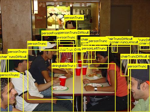
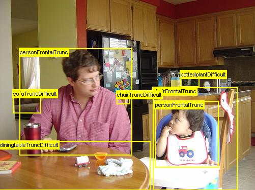
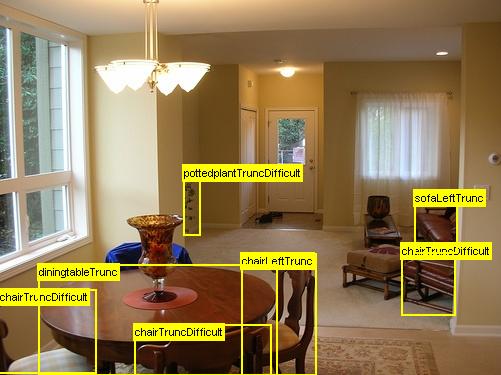
Figure 6: Examples from the PASCAL VOC dataset. Fig.6 and Fig.6 contain three categories: people, table and chair. Fig.6 contains table and chair.

In his experiment, we choose the most common combination of three categories: person, chairs and dining table. Objects labeled as difficult for object classification are not used in our experiments.

For the experiments, we repeatedly sample sets of images containing one, two, and three categories. The training/validation set and testing set have the same distribution. For a single iteration, we sample 480 images for the training/validation set including 30 images with all labels, and 150 images each for sets containing zero, one, or two of the target labels. More than 5,000 images from the entire dataset are sampled at least once as we repeat the experiments with random samplings to compute statistical significance. In this task, we first define the submodular loss function as follows:

$$\Delta_{2}(y,\tilde{y}):=\min\left(l_{\textrm{max}},\left\langle\beta,(1-y\odot\tilde{y})/2\right\rangle\right)$$ (51)

where $\odot$ is the Hadamard product, $l_{\textrm{max}}$ is the maximal risk value, $\beta>0$ is a coefficient vector of size $p$ that accounts for the relative importance of each category label. $l_{max}<\|\beta\|_{1}$ ensures the function is strictly submodular. This function is an analogue to the submodular increasing function in Sec. 4.4. In this VOC experiments, we order the category labels as person, dining table and chair. We set $l_{\textrm{max}}=1.3$ and $\beta=[1\ 0.5\ 0.2]$.

We have additionally carried out experiments with another submodular loss function:

$$\Delta_{3}(y,\tilde{y}):=1-\exp\left(-|\mathbf{I}|\right)+\left\langle\beta,(1-y\odot\tilde{y})/2\right\rangle$$ (52)

where $\mathbf{I}=\{j|\tilde{y}^{j}\neq y^{j}\}$ is the set of mispredicted labels. The first part, $1-\exp\left(-|\mathbf{I}|\right)$, is a concave function depending only on the size of $\mathbf{I}$, as a consequence it is a submodular function; the second part is a modular function that penalizes labels proportionate to the coefficient vector $\beta$ as above. The results with this submodular loss are shown in Table III. We additionally train and test with the 0-1 loss, which is equivalent to an SVM.

We compare different losses employed during training and during testing. $\mathbf{M}$ and $\mathbf{S}$ denote the use of the submodular loss with margin and slack rescaling, respectively. The empirical results with this submodular loss are shown in Table III.

TABLE III: For the VOC multilabel prediction task, the cross comparison of average loss values (with standard error) using submodular loss as in Equation (51) and Equation (52), as well as 0-1 loss during training and during testing.

		Test
		$\Delta_{2}$	0-1
Train	$\mathbf{L}$	$\mathbf{0.4371\pm 0.0045}$	$0.9329\pm 0.0097$
	0-1	$0.5091\pm 0.0023$	$\mathbf{0.8320\pm 0.0074}$
	$\mathbf{S}$	$0.4927\pm 0.0067$	$0.8731\pm 0.0073$
	$\mathbf{M}$	$0.4437\pm 0.0034$	$1.0010\pm 0.0080$

		Test
		$\Delta_{3}$	0-1
Train	$\mathbf{L}$	$\mathbf{0.9447\pm 0.0069}$	$0.8786\pm 0.0077$
	0-1	$0.9877\pm 0.0044$	$\mathbf{0.8173\pm 0.0061}$
	$\mathbf{S}$	$0.9784\pm 0.0052$	$0.8337\pm 0.0054$
	$\mathbf{M}$	$0.9718\pm 0.0041$	$0.9425\pm 0.0054$

6.4 Microsoft COCO multilabel prediction

In this section, we consider the multi-label prediction task on Microsoft COCO dataset. On detecting a dinner scene, the initial multi-label prediction should emphasize that all labels must be correct within a given image, while MS COCO provides more relating categories e.g. people, dinning tables, forks or cups. Submodular loss functions coincides with the fact that misprediction of a single label, e.g. person, will preclude the chance to predict correctly the combination of all labels. Fig. 7 shows example images from the Microsoft COCO dataset [36].

Figure 7: Examples from the Microsoft COCO dataset. Fig. 7 contains all the categories of interest (cf. Section 6); Fig. 7 contains dining table, fork and cup; Fig. 7 is not a dining scene but contains people.

The Microsoft COCO dataset [36] is an image recognition, segmentation, and captioning dataset. It contains more than 70 categories, more than 300,000 images and around 5 captions per image. We have used frequent itemset mining [37] to determine the most common combination of categories in an image. For sets of size 6, these are: person, cup, fork, knife, chair and dining table.

For the experiments, we repeatedly sample sets of images containing $k$ ($k=0,1,2,\cdots,6$) categories. The training/validation set and testing set have the same distribution. For a single iteration, we sample 1050 images for the training/validation set including 150 images each for sets containing $k$ ($k=0,1,2,\cdots,6$) of the target labels. More than 12,000 images from the entire dataset are sampled at least once as we repeat the experiments to compute statistical significance.

In this task, we first use a submodular loss function as follows:

$$\Delta_{4}(y,\tilde{y}):=1-\exp\left(-\alpha|\mathbf{I}|\right)$$ (53)

where $\mathbf{I}=\{j|y^{j}\neq\tilde{y}^{j}\}$ is the set of mispredicted labels. $1-\exp\left(-|\mathbf{I}|\right)$, is a concave function depending only on the size of $\mathbf{I}$, as a consequence it is a submodular function, $\alpha$ is a positive coefficient that effect the increasing rate of the concave function thus the submodularity of the set function. In the experiment we set $\alpha=1$ (cf. Table IV).

We have also carried out experiments with the submodular loss function used in VOC experiments:

$$\Delta_{5}(y,\tilde{y}):=1-\exp\left(-|\mathbf{I}|\right)+\left\langle\beta,(1-y\odot\tilde{y})/2\right\rangle$$ (54)

where we set $\beta=[1\ 0.8\ 0.7\ 0.6\ 0.5\ 0.4]^{T}$ according to the size of the object that we order the category labels as person, dining table, chair, cup, fork and knife (cf. Table IV).

In addition, we use another submodular loss, which is a concave over modular function, as follows,

$$\Delta_{6}(y,\tilde{y}):=\sqrt{m(\mathbf{I})}$$ (55)

where $m$ is a modular function for which the values on each element is defined as

$$m(\{j\})=\sum_{A\in F}[j\in A].$$ (56)

where the $F$ is the set of frequent itemsets that has been pre-calculated among training samples. This loss gives a higher penalty for mispredicting clustered labels that frequently co-occur in the training set (cf. Table IV). While the diminishing returns property of submodularity yields the correct cluster semantics: if we already have a large set of mispredctions, the joint prediction is already poor and an additional misprediction has a lower marginal cost.

We compare different losses employed during training and during testing. We also train and test with the 0-1 loss, which is equivalent to an SVM. $\mathbf{M}$ and $\mathbf{S}$ denote the use of the submodular loss with margin and slack rescaling, respectively. As this optimization is NP-hard, we have employed the simple application of the greedy approach as is common in (non-monotone) submodular maximization (e.g. [38]).

We repeated each experiment 10 times with random sampling in order to obtain an estimate of the average performance. Table IV shows the cross comparison of average loss values (with standard error) using different loss functions during training and during testing for the COCO dataset.

6.5 Empirical Results

From the empirical results in Table I, Table II, Table III and Table IV, we can see that training with the same submodular loss functions as used during testing yields the best results. Slack and margin rescaling fail due to the necessity of approximate inference, which results in a poor discriminant function. By contrast, the Lovász hinge yields the best performance when the submodular loss is used to evaluate the test predictions. We do not expect that optimizing the submodular loss should give the best performance when the 0-1 loss is used to evaluate the test predictions. Indeed in this case, the Lovász hinge trained on 0-1 loss corresponds with the best performing system.

Fig. 8 and Fig. 8 show for the two submodular functions the primal-dual gap as a function of the number of cutting-plane iterations using the Lovász hinge with submodular loss, as well as for a SVM (labeled 0-1), and margin and slack rescaling (labeled $\mathbf{M}$ and $\mathbf{S}$). This demonstrates that the empirical convergence of the Lovász hinge is at a rate comparable to an SVM, and is feasible to optimize in practice for real-world problems.

TABLE IV: For the MS COCO prediction task, the comparison of average loss values (with standard error) using the submodular losses as in Equation (53), Equation (54) and Equation (55), as well as 0-1 loss during training and during testing.

		Test
		$\Delta_{4}$	0-1
Train	$\mathbf{L}$	$\mathbf{0.5567\pm 0.0057}$	$1.4295\pm 0.0194$
	0-1	$0.5729\pm 0.0060$	$\mathbf{1.3924\pm 0.0195}$
	$\mathbf{S}$	$0.5875\pm 0.0065$	$1.4940\pm 0.0233$
	$\mathbf{M}$	$0.5820\pm 0.0063$	$1.4802\pm 0.0233$

		Test
		$\Delta_{5}$	0-1
Train	$\mathbf{L}$	$\mathbf{1.3767\pm 0.0143}$	$1.3003\pm 0.0176$
	0-1	$1.3813\pm 0.0135$	$\mathbf{1.2975\pm 0.0152}$
	$\mathbf{S}$	$1.4711\pm 0.0153$	$1.3832\pm 0.0156$
	$\mathbf{M}$	$1.4811\pm 0.0117$	$1.4016\pm 0.0136$

		Test
		$\Delta_{6}$	0-1
Train	$\mathbf{L}$	$\mathbf{0.6141\pm 0.0048}$	$1.2504\pm 0.0106$
	0-1	$0.6224\pm 0.0048$	$\mathbf{1.2461\pm 0.0115}$
	$\mathbf{S}$	$0.6700\pm 0.0051$	$1.3789\pm 0.0150$
	$\mathbf{M}$	$0.6723\pm 0.0051$	$1.3787\pm 0.0123$

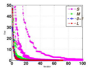
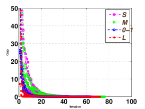
Figure 8: The primal-dual gap as a function of the number of cutting-plane iterations using the Lovász hinge with submodular loss, a SVM (labeled 0-1), and margin and slack rescaling with greedy inference (labeled $m_{sub}$ and $s_{sub}$). Fig. 8 for the experiment using Equation (53) and Fig. 8 for Equation (54). This demonstrates that empirical convergence of the Lovász hinge is at a rate comparable to an SVM, and is feasible to optimize in practice for real-world problems.

7 Discussion & Conclusion

In this work, we have introduced a novel convex surrogate loss function, the Lovász hinge, which makes tractable for the first time learning with submodular loss functions. In contrast to margin and slack rescaling, computation of the gradient or cutting plane can be achieved in $\mathcal{O}(p\log p)$ time. Margin and slack rescaling are NP-hard to optimize in this case, and furthermore deviate from the convex closure of the loss function (Corollary 1).

We have proven necessary and sufficient conditions for margin and slack rescaling to yield tight convex surrogates to a discrete loss function. These conditions are that the discrete loss be a (properly scaled) increasing function. However, it may be of interest to consider non-monotonic functions in some domains. The Lovász hinge can be applied also to non-monotonic functions.

We have demonstrated the correctness and utility of the Lovász hinge on different tasks. We have shown that training by minimization of the Lovász hinge applied to multiple submodular loss functions, including the popular Jaccard loss, results in a lower empirical test error than existing methods, as one would expect from a correctly defined convex surrogate. Slack and margin rescaling both fail in practice as approximate inference does not yield a good approximation of the discriminant function. The causes of this have been studied in a different context in [39], but are effectively due to (i) repeated approximate inference compounding errors, and (ii) erroneous early termination due to underestimation of the primal objective. We empirically observe that the Lovász hinge delivers much better performance by contrast, and makes no approximations in the subgradient computation. Exact inference should yield a good predictor for slack and margin rescaling, but sub-exponential optimization only exists if P=NP. Therefore, the Lovász hinge is the only polynomial time option in the literature for learning with such losses.

The introduction of this novel strategy for constructing convex surrogate loss functions for submodular losses points to many interesting areas for future research. Among them are then definition and characterization of useful loss functions in specific application areas. Furthermore, theoretical convergence results for a cutting plane optimization strategy are of interest.

Acknowledgements

This work is partially funded by Internal Funds KU Leuven, ERC Grant 259112, and FP7-MC-CIG 334380. The first author is supported by a fellowship from the China Scholarship Council.

References

- [1] J. Yu and M. B. Blaschko, “Learning submodular losses with the Lovász hinge,” in Proceedings of the 32nd International Conference on Machine Learning, ser. JMLR Proceedings, vol. 37, 2015, pp. 1623–1631.
- [2] P. L. Bartlett, M. I. Jordan, and J. D. McAuliffe, “Convexity, classification, and risk bounds,” Journal of the American Statistical Association, vol. 101, no. 473, pp. 138–156, 2006.
- [3] I. Tsochantaridis, T. Joachims, T. Hofmann, and Y. Altun, “Large margin methods for structured and interdependent output variables,” Journal of Machine Learning Research, vol. 6, no. 9, pp. 1453–1484, 2005.
- [4] D. McAllester, “Generalization bounds and consistency for structured labeling,” in Predicting Structured Data. MIT Press, 2007.
- [5] A. Tewari and P. L. Bartlett, “On the consistency of multiclass classification methods,” The Journal of Machine Learning Research, vol. 8, pp. 1007–1025, 2007.
- [6] M. B. Blaschko and C. H. Lampert, “Learning to localize objects with structured output regression,” in European Conference on Computer Vision, ser. Lecture Notes in Computer Science, D. Forsyth, P. Torr, and A. Zisserman, Eds., 2008, vol. 5302, pp. 2–15.
- [7] S. Nowozin, “Optimal decisions from probabilistic models: The intersection-over-union case,” in Proceedings of the IEEE Conference on Computer Vision and Pattern Recognition, 2014.
- [8] W. Cheng, E. Hüllermeier, and K. J. Dembczynski, “Bayes optimal multilabel classification via probabilistic classifier chains,” in Proceedings of the International Conference on Machine Learning, 2010, pp. 279–286.
- [9] J. Petterson and T. S. Caetano, “Submodular multi-label learning,” in Advances in Neural Information Processing Systems, 2011, pp. 1512–1520.
- [10] C.-L. Li and H.-T. Lin, “Condensed filter tree for cost-sensitive multi-label classification,” in Proceedings of the 31st International Conference on Machine Learning, 2014, pp. 423–431.
- [11] J. R. Doppa, J. Yu, C. Ma, A. Fern, and P. Tadepalli, “HC-search for multi-label prediction: An empirical study,” in Proceedings of AAAI Conference on Artificial Intelligence, 2014.
- [12] J. Díez, O. Luaces, J. J. del Coz, and A. Bahamonde, “Optimizing different loss functions in multilabel classifications,” Progress in Artificial Intelligence, vol. 3, no. 2, pp. 107–118, 2015.
- [13] W. Gao and Z.-H. Zhou, “On the consistency of multi-label learning,” Artificial Intelligence, vol. 199, pp. 22–44, 2013.
- [14] F. Bach, “Structured sparsity-inducing norms through submodular functions,” in Advances in Neural Information Processing Systems, 2010, pp. 118–126.
- [15] R. Iyer and J. Bilmes, “The Lovász-Bregman divergence and connections to rank aggregation, clustering, and web ranking: Extended version,” Uncertainity in Artificial Intelligence, 2013.
- [16] V. N. Vapnik, The Nature of Statistical Learning Theory. Springer, 1995.
- [17] S. Fujishige, Submodular functions and optimization. Elsevier, 2005.
- [18] B. Taskar, C. Guestrin, and D. Koller, “Max-margin markov networks,” in Advances in Neural Information Processing Systems 16, S. Thrun, L. K. Saul, and B. Schölkopf, Eds. MIT Press, 2004, pp. 25–32.
- [19] A. Criminisi and J. Shotton, Decision Forests for Computer Vision and Medical Image Analysis. Springer, 2013.
- [20] Y. Bengio, “Learning deep architectures for AI,” Found. Trends Mach. Learn., vol. 2, no. 1, pp. 1–127, Jan. 2009.
- [21] T. Hastie, R. Tibshirani, and J. Friedman, The elements of statistical learning: Data mining, inference and prediction, 2nd ed. Springer, 2009.
- [22] G. L. Nemhauser, L. A. Wolsey, and M. L. Fisher, “An analysis of approximations for maximizing submodular set functions–I,” Mathematical Programming, vol. 14, no. 1, pp. 265–294, 1978.
- [23] L. Lovász, “Submodular functions and convexity,” in Mathematical Programming The State of the Art. Springer, 1983, pp. 235–257.
- [24] J. Edmonds, “Matroids and the greedy algorithm,” Mathematical programming, vol. 1, no. 1, pp. 127–136, 1971.
- [25] F. Bach, “Learning with submodular functions: A convex optimization perspective,” Foundations and Trends in Machine Learning, vol. 6, no. 2-3, pp. 145–373, 2013.
- [26] R. K. Iyer and J. A. Bilmes, “Polyhedral aspects of submodularity, convexity and concavity,” Arxiv, CoRR, vol. abs/1506.07329, 2015.
- [27] J. Strayer, Linear Programming and Its Applications. Springer, 1989.
- [28] G. Choquet, “Theory of capacities,” Annales de l’institut Fourier, vol. 5, pp. 131–295, 1954.
- [29] T. Joachims, T. Finley, and C.-N. Yu, “Cutting-plane training of structural SVMs,” Machine Learning, vol. 77, no. 1, pp. 27–59, 2009.
- [30] D. Liben-Nowell and J. Kleinberg, “The link-prediction problem for social networks,” Journal of the American society for information science and technology, vol. 58, no. 7, pp. 1019–1031, 2007.
- [31] R. Unnikrishnan, C. Pantofaru, and M. Hebert, “Toward objective evaluation of image segmentation algorithms,” Pattern Analysis and Machine Intelligence, IEEE Transactions on, vol. 29, no. 6, pp. 929–944, 2007.
- [32] M. Everingham, L. Van Gool, C. K. Williams, J. Winn, and A. Zisserman, “The Pascal visual object classes (VOC) challenge,” pp. 303–338, 2010.
- [33] O. Russakovsky, J. Deng, H. Su, J. Krause, S. Satheesh, S. Ma, Z. Huang, A. Karpathy, A. Khosla, M. S. Bernstein, A. C. Berg, and F. Li, “ImageNet large scale visual recognition challenge,” CoRR, vol. abs/1409.0575, 2014.
- [34] P. Sermanet, D. Eigen, X. Zhang, M. Mathieu, R. Fergus, and Y. LeCun, “Overfeat: Integrated recognition, localization and detection using convolutional networks,” in International Conference on Learning Representations, 2014.
- [35] A. S. Razavian, H. Azizpour, J. Sullivan, and S. Carlsson, “CNN features off-the-shelf: An astounding baseline for recognition,” in IEEE Conference on Computer Vision and Pattern Recognition Workshops, 2014, pp. 512–519.
- [36] T. Lin, M. Maire, S. Belongie, J. Hays, P. Perona, D. Ramanan, P. Dollár, and C. L. Zitnick, “Microsoft COCO: common objects in context,” CoRR, vol. abs/1405.0312, 2014.
- [37] T. Uno, T. Asai, Y. Uchida, and H. Arimura, “An efficient algorithm for enumerating closed patterns in transaction databases,” in Discovery Science. Springer, 2004, pp. 16–31.
- [38] A. Krause and D. Golovin, “Submodular function maximization,” in Tractability: Practical Approaches to Hard Problems, L. Bordeaux, Y. Hamadi, and P. Kohli, Eds. Cambridge University Press, 2014.
- [39] T. Finley and T. Joachims, “Training structural SVMs when exact inference is intractable,” in Proceedings of the 25th International Conference on Machine Learning, 2008, pp. 304–311.