On the composition dependence of thermodynamic, dynamic and dielectric properties of water-methanol model mixtures. Molecular dynamics
simulation results

Abstract

We have investigated thermodynamic and dynamic properties as well as the dielectric constant of water-methanol model mixtures in the entire range of composition by using constant pressure molecular dynamics simulations at ambient conditions. The SPC/E and TIP4P/Ew water models are used in combination with the OPLS united atom modelling for methanol. Changes of the average number of hydrogen bonds between particles of different species and of the fractions of differently bonded molecules are put in correspondence with the behavior of excess mixing volume and enthalpy, of self-diffusion coefficients and rotational relaxation times. From the detailed analyses of the results obtained in this work, we conclude that an improvement of the description of an ample set of properties of water-methanol mixtures can possibly be reached, if a more sophisticated, carefully parameterized, e.g., all atom, model for methanol is used. Moreover, exploration of parametrization of the methanol force field, with simultaneous application of different combination rules for methanol-water cross interactions, is required.

Key words: water models, methanol models, thermodynamic properties, translational and orientational diffusion, dielectric constant, molecular dynamics

PACS: 61.20.-p, 61.20-Gy, 61.20.Ja, 65.20.Jk

Abstract

Нами дослiджено термодинамiчнi та динамiчнi властивостi, а також дiелектричну сталу модельних сумiшей вода-метанол у всьому дiапазонi концентрацiй з використанням симуляцiй методом молекулярної динамiки при постiйному тиску i в довкiльних умовах. Використано моделi води SPC/E i TIP4P/Ew у поєднаннi з OPLS об’єднаним атомним моделюванням для метанолу. Змiни середнього числа водневих зв’язкiв мiж частинками рiзних сортiв та фракцiй по-рiзному зв’язаних молекул поставлено у вiдповiднiсть з поведiнкою об’єму надлишкового змiшування та ентальпiї, коефiцiєнтiв самодифузiї та часiв ротацiйної релаксацiї. Детально проаналiзувавши отриманi в роботi результати, робимо висновок, що можна досягнути певного вдосконалення опису великої кiлькостi властивостей сумiшей вода-метанол за умови використання бiльш складної, ретельно параметризованої, наприклад, повнiстю атомної моделi. До того ж, iснує потреба у дослiдженнi параметризацiї силового поля метанолу з одночасним використанням рiзних комбiнацiйних правил для взаємодiй метанол-вода.

Ключовi слова: моделi води, моделi метанолу, термодинамiчнi властивостi, трансляцiйна та орiєнтацiйна дифузiя, дiелектрична стала, молекулярна динамiка

1 Introduction

In the very recent work from this laboratory we reported a detailed analysis of molecular dynamics computer simulation data for the microscopic structure of water-methanol mixtures in the entire composition range, and performed comparisons with experimental results obtained using X-ray diffraction [1]. Our principal focus in that publication was on the changes, with composition, of the experimental and theoretical total structure factors of mixtures considered at room temperature and ambient pressure. On the molecular dynamics (MD) side, we analyzed the SPC/E [2] and the TIP4P/Ew [3] water models combined with the OPLS/AA (all atom) methanol model [4]. The all atom modelling for methanol was used in that study because it is intrinsically required by the procedure to perform comparisons with the experimental total structure factors.

Encouraged by an overall satisfactory performance of the MD simulation data in the description of the experimental trends, in the present work our primary objective is to extend our previous study by exploring the results for a more comprehensive set of properties of water-methanol mixtures, besides the microscopic structure. Namely, we focus on thermodynamic, dynamic and dielectric properties obtained from our MD simulations and perform comparisons with the available experimental data. Results of computer simulations from other authors are included as well, aiming at a more comprehensive insight into the dependence of properties of mixtures in question on the conditions of computer modelling.

There have been very many studies of water-alcohol mixtures, and of water-methanol mixtures in particular, with the use of computer simulation methods since the pioneering works by Jorgensen and Madura [5] and by Okazaki et al. [6, 7], principally focused on ‘‘infinite dilution’’ solutions by considering a single methanol molecule in a set of water molecules. The results were obtained using Monte Carlo (MC) simulations in the NPT and NVT ensemble, respectively. To our best knowledge, Ferrario et al. [8] and Tanaka with Gubbins [9] were the first to report thermodynamic and dynamic properties of these systems in the entire composition range from MD and MC simulations, respectively. Since then, much knowledge has been accumulated about the properties of water-methanol mixtures, see e.g., [10, 11, 12, 13]. In particular, one of the more recent works on the topic, with the principal focus on dynamic properties of water-alcohol mixtures (methanol, ethanol and 1-propanol) using the TIP4P water model [14] in combination with the OPLS/AA model for alcohols [4] has been published by Wensink et al. [15]. On the other hand, Guevara-Carrion et al. [16] explored the SPC/E and TIP4P-2005 [17] water models in combination with a united atom type methanol model [18] for mixtures, reporting excess mixing volume and enthalpy, self-diffusion coefficients, shear viscosity and power spectra. Recent works on water-methanol mixtures include detailed studies of the mixing volume and mixing enthalpy [19, 20], using the NPT MC simulations.

Analyses of various results emerging from computer simulations by using non-polarizable water models and different versions of force fields for alcohols in comparison with experimental data clearly show the necessity of further work. Namely, it seems necessary to reach a systematic, more profound understanding of strengths and drawbacks of different models and provide a design aiming at a better agreement with experiments, desirably for an ample set of properties of mixtures of interest, rather than for a single particular property.

In this respect, in the present work we would like to report thermodynamic properties of mixing in terms of excess mixing volume and excess mixing enthalpy, a set of dynamic properties that include the self-diffusion coefficients and rotational relaxation times, as well as the dielectric constant, all together with the detailed analysis of hydrogen bonding within species and between them, in the entire range of composition, starting from pure water and terminating by pure methanol. Whenever possible, we discuss the results of other authors and make comparisons with experimental data from literature. We restrict our attention to two different water models and the OPLS/UA (united atom) potential model of methanol in order to establish their performance. The OPLS/UA model for methanol and other more complex alcohols is popular in comparison with the more detailed OPLS/AA model due to computational efficiency.

Several recent efforts have focused on the parametrization of different properties of water, see e.g., [21, 22], targeting to improve the description of the dielectric constant and of the density anomaly. A similar approach has been applied to methanol at the united atom level, see [23], targeting the dielectric constant in particular. The strategy of the proposed parametrization includes scaling of site charges with the dielectric constant as a target, and scaling of the energy of non-bonded interactions leading to a corrected surface tension as subsequent steps. The critical temperature is used for control as well. The parametrization can be done in cycles to yield correct values for the targets. On the other hand, Schnabel et al. [18] developed a successful parametrization of the OPLS/UA type model for methanol using vapor-liquid equilibrium data, focusing on the correct description of the hydrogen bonds statistics to correctly reproduce the nuclear magnetic resonance spectroscopic data.

2 Simulation details

All our simulations of water-methanol mixtures models were performed in the isothermal-isobaric ensemble at ambient pressure. The present work involves exploration of two commonly used water models, namely the SPC/E [2] and the TIP4P/Ew ones [3]. On the other hand, the OPLS/UA (united atom) rigid nonpolarizable model for methanol [24] in the present work is taken with the adjusted parameters of [25]. The OPLS/UA model for methanol has been designed so that the parameters of the nonbonded potentials between different types of atoms satisfy the geometric combination rules [24]. However, in the work of van Leeuwen and Smith [25], new parameters for nonbonded potentials were designed and standard Lorentz-Berthelot (LB) combination rules, i.e., $\epsilon_{ij}=(\epsilon_{ii}\epsilon_{jj})^{1/2}$ and $\sigma_{ij}=(\sigma_{ii}+\sigma_{jj})/2$, were used to calculate the liquid-vapor coexistence curve of methanol and a bit later of other alkanols [26]. Again, the LB combination rules were used for methanol in [27].

This is a setup similar to the one recently used by Moučka and Nezbeda [20], and we just apply the SPC/E and TIP4P/Ew models instead of the TIP4P potential considered by these authors. Moreover, we have not done any deviation from the LB combination rules, in contrast to [20]. All the simulations of water-OPLS/UA version of the models, unless specified, were performed using the DLPOLY Classic package [28]. We used the Berendsen thermostat and barostat with $\tau_{T}=0.1$ ps and $\tau_{P}=2.0$ ps, the running timestep was 0.002 ps. As common, periodic boundary conditions were used. The nonbonded interactions were cut-off at 11 Å, whereas the long-range interactions were handled by the Ewald method with a precision of $10^{-5}$. In order to maintain the geometry of water and methanol molecules, the SHAKE algorithm was used. For all simulations, the initial configurations were constructed by using from 2000 to 3000 molecules of the two species placed randomly in a cubic box. After equilibration, several sets of simulation runs were performed, each lasting for 6–8 ns, with restart from the previous configuration, to obtain the averages for data analysis. Actually, the overall length of simulation was dictated by the stability of internal energy, density and the dielectric constant, so that the runs were not shorter than 20 ns. The precise numbers of molecules of both species used in our simulations are given in table 1. Changes of the mixture compositions (as well as the compositions themselves) throughout this study are described by $X_{\textrm{m}}$ (molar fraction of methanol); its values are given in table 1 as well. In addition, we provide the weight concentration of methanol for convenience of the reader.

Table 1: The number of molecules of water and methanol in MD simulations, molar fraction and weight concentration of methanol.

$N_{\textrm{w}}$	$N_{\textrm{m}}$	​ $X_{\textrm{m}}$	wt${}_{\textrm{m}}$ (%)
2000	0	0	0
2000	125	0.06	10
2000	281	0.12	20
1898	457	0.19	30
1800	674	0.27	40
1600	899	0.41	50
1600	1099	0.46	55
1600	1349	0.51	60
1400	1462	0.57	65
1200	1574	0.63	70
1200	1855	0.63	75
1100	1800	0.69	80
800	2230	0.76	85
700	2100	0.84	90
415	2670	0.91	95
0	2100	1.00	100

3 Results and discussion

First we would like to discuss our observations concerning the properties that do not require any reference to the species forming the mixture (such as overall density, mixing properties and the dielectric constant) and next proceed to the properties characterizing individual species characteristics such as self-diffusion coefficients and reorientational relaxation times, and discuss hydrogen bonding in terms of the average number of bonds per molecule of the particular species, cross bonds and bonding states of molecules of each species.

3.1 Density, mixing properties and the dielectric constant

Changes of the liquid mixture density with methanol mole fraction for the two combinations of potential models are shown in figure 1. The NPT molecular dynamics simulation data at room temperature (298.15 K) and at ambient pressure are accompanied by the experimental values [29]. The SPC/E-OPLS/UA model very well reproduces the experimental results. Only at high methanol fractions, the mixture density is slightly overestimated in comparison with the experimental data but this disagreement is hardly visible on the scale of the figure. It is worth mentioning that if the methanol component is described within the OPLS/AA model, then the density of the mixtures in question is described less satisfactorily: it is underestimated practically in the entire composition range [1]. To conclude with this figure, it seems that the united atom model for methanol is reliable to describe changes of the density on composition of the mixture at room temperature and at ambient pressure.

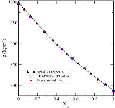
Figure 1: (Color online) Composition dependence of the water-methanol mixture density from the present NPT simulations of the SPC/E-OPLS/UA and TIP4P/Ew-OPLS/UA models, together with experimental results [29]. The nomenclature of lines and symbols is given in the figure.

However, a more sensitive test for the species modelling is illustrated by the calculations of the excess mixing volume, $\Delta V_{\textrm{mix}}$, figure 2. It is obtained straightforwardly as: $\Delta V_{\textrm{mix}}=V_{\textrm{mix}}-(1-X_{\textrm{m}})V_{\textrm{w}}-X_{\textrm{m}}V_{\textrm{m}}$. At the united atom level of modelling, changes of the water model yield a marginal improvement of the composition dependence of $\Delta V$ with respect to the experimental data [30]. Actually, the results are reasonably good for both water-rich and methanol-rich mixtures compared to the experiment. However, at the intermediate region, the applied modelling underestimates the nonideality of mixtures. Similar trends (to underestimate nonideality) have been observed for the TIP4P-OPLS/UA combination of models, if the geometric mixing rules were used for the cross-energies and cross-diameters [19], cf. figure 1 (a) of reference [19]. Moreover, the overall performance of the excess mixing volume coming from simulations does not improve for different explored sets of deviation parameters from the standard LB combination rules as shown by [20] for the TIP4P-OPLS/UA model, cf. figure 2 of reference [20]. Our figure 2 complements the results shown in figure 15 of reference [16]. Summarizing our results and insights coming from the previous simulations in [16, 19, 20], it seems that different combinations of water and methanol models yield a satisfactory description of the excess mixing volume and correctly predict the composition value, $X_{\textrm{m}}\approx 0.5$ at which $\Delta V_{\textrm{mix}}$ is minimum. However, it is doubtful whether such a moderate success would be preserved for other temperatures and pressures and/or for other water-alcohol mixtures. Therefore, accumulation of knowledge about the performance of different models under other conditions and for other members of water-alcohol mixtures family is of great importance. On the other hand, it seems necessary to explore parametrization and/or sophistication of the OPLS/AA modelling, placing the focus on this particular experimentally measurable property.

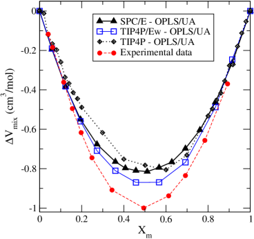
Figure 2: (Color online) Excess mixing volume of water-methanol mixtures on methanol molar fraction for united atom modelling from our NPT molecular dynamics and the results from Monte Carlo simulations [19] for the TIP4P-OPLS/UA model, versus experimental data [30].

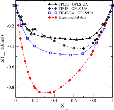
Figure 3: (Color online) Excess mixing enthalpy of water-methanol mixtures on methanol molar fraction for united atoms modelling versus experimental data [31].

The excess enthalpy of mixing, $\Delta H_{\textrm{mix}}$ is determined as follows:

$$\Delta H_{\textrm{mix}}=H_{\textrm{mix}}-(1-X_{\textrm{m}})H_{\textrm{w}}-X_{\textrm{m}}H_{\textrm{m}}\,,$$ (1)

where $H_{\textrm{mix}}$ is $U_{\textrm{pot}}+PV$. As we see from the curves in figure 3 and from experimental results [31], the behavior predicted by simulations with either water models of this study, combined with OPLS/UA, is not satisfactory. On the methanol-rich side, the behavior of the theoretical curves seems to be a little better than on the water-rich side. However, in the entire range of compositions, computer modelling yields much weaker effects of nonideality compared to the experimental data. Moreover, the minimum of $\Delta H_{\textrm{mix}}$ from simulations is seen at a higher methanol fraction compared to the experimental results. These observations are in line with the previous studies using, for instance, the TIP4P-2005 water model and the parameterized methanol model, cf. figure 16 of reference [16], and figures 1 (b), 2 (b) of reference [19]. This behavior points out that the energetic aspects of mixing methanol and water in simulations should be reconsidered. A growth of the absolute value for $\Delta H_{\textrm{mix}}$ can be reached by employing certain deviations to the combination rules [20], but then the position of the minimum for $\Delta H_{\textrm{mix}}$ shifts to methanol-rich mixtures, which is in contradiction to the experimental behavior. Thus, it does not seem that the combination rules are responsible for this type of failure. One can hope that modelling of methanol at the all atom level would be profitable to improve an agreement with experimental data for this particular property. However, another possibility is that nonpolarizable models are intrinsically incapable of providing a desired agreement for this particular property. Definitely, other characteristics of the system that involve potential energy, besides excess mixing enthalpy, should be explored to make stronger conclusions.

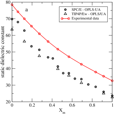
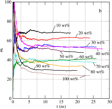
Figure 4: (Color online) Panel (a): Composition dependence of the dielectric constant of water-methanol mixture from our present simulations versus experimental data [35]. The nomenclature of lines and symbols is given in the inset. Panel (b): Time dependence of the dielectric constant at different weight concentration.

Now we proceed to another property that, as seen below, is not very successfully described within the framework of the potential models applied. It is known that the long-range, asymptotic behavior of correlation functions between molecules possessing dipole moments is described by the dielectric constant, $\varepsilon$. In general terms, the calculation of the dielectric constant from simulations is a demanding task, see e.g., [21, 32, 33] for the discussion of calculations of $\varepsilon$ for pure water. Several factors can influence the result, such as the number of molecules, type of thermostat and barostat, precision of the summation of long-range interactions. Moreover, long runs are necessary to obtain reasonable estimates for this property, since it is usually calculated from the time-average of the fluctuations of the total dipole moment of the system [34] as follows:

$$\varepsilon=1+\frac{4\pi}{3k_{\textrm{B}}TV}\left(\langle{\bf M}^{2}\rangle-\langle{\bf M}\rangle^{2}\right),$$ (2)

where $k_{\textrm{B}}$ is the Boltzmann constant and V is the simulation cell volume.

Both of the models for the pure species, water and methanol, are perfect in predicting their respective dielectric constants. As a result, the behavior of mixtures in the entire composition range is not perfect either, figure 4 (a). The inclination of the curve for $\varepsilon(X_{\textrm{m}})$ is not bad at all, but the values are too low compared to the experimental results. We get confidence in the quality of the present results making long simulations [figure 4 (b)] with a sufficiently large number of particles in the simulation box. A simultaneous improvement of water and methanol models is necessary to obtain better values of the dielectric constant for the mixtures in question. How good is the parametrization of the methanol model of [18] with respect to the dielectric constant is unknown so far. On the other hand, quite recently the united atom model of methanol was parameterized to reproduce the experimental value of the dielectric constant [23], at the expense of making other properties worse, e.g., the self-diffusion coefficient. However, the performance of this modified model for water-methanol mixtures has not been evaluated yet. We plan to improve the description of the dielectric constant by performing simulations for more sophisticated models. Without such efforts it is difficult to attempt a successful description of the thermodynamics and the dynamics of ionic solvation in mixed water-alcohol solvents.

3.2 Dynamic properties and hydrogen bonding

We proceed to the description of our results for a set of dynamic properties. The self-diffusion coefficients for the two species of the mixture were calculated by two routes. Namely, from the mean-square displacement (MSD) of a particle via the Einstein relation,

$$D_{i}=\frac{1}{6}\lim_{t\rightarrow\infty}\frac{\mathrm{d}}{\mathrm{d}t}\langle|{\bf r}_{i}(t)-{\bf r}_{i}(0)|^{2}\rangle,$$ (3)

where $i$ refers to water or methanol species. The MSD procedure to obtain $D_{i}$ was applied by using particle coordinates coming from DLPOLY simulations. On the other hand, we also obtained the self-diffusion coefficients from the time integral of the velocity autocorrelation functions,

$$D_{i}=\frac{1}{3}\int_{0}^{\infty}\mathrm{d}t\langle{\bf v}_{i}(t){\cdot}{\bf v}_{i}(0)\rangle.$$ (4)

For this purpose we employed the GROMACS software for the same model and with the same technical setup as in the DLPOLY package. This has been done due to the speed efficiency of GROMACS. For the sake of checking mutual consistency, a set of calculations has been performed and the results are given in figure 5. We observe that the two procedures yield very similar results, margins of inaccuracy overlap for all compositions.

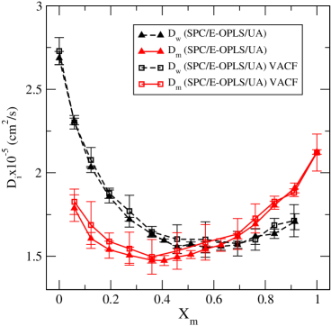
Figure 5: (Color online) A comparison of self-diffusion coefficients of the two species coming from mean square displacements calculations and from the velocity autocorrelation functions. Error bars are shown. The subscripts ‘‘m’’ and ‘‘w’’ refer to methanol and water, respectively.

A set of results for self-diffusion coefficients coming from simulations by using VACF is given in figure 6. While an overall behavior of the curves for water and methanol molecules is correct, the experimental [36] and simulation data differ in several details. On the water-rich side, the simulation data overestimate the self-diffusion coefficients as a result of inability of the explored models for water to yield the self-diffusion coefficient in perfect agreement with the experimental value for pure water. The self-diffusion coefficient for pure methanol is not as bad. The OPLS/UA model slightly underestimates the self-diffusion coefficient value. However, the minima of the curves for each species of the mixtures are less pronounced than in the experiment. Moreover, the crossing point where the self-diffusion coefficient of water and methanol molecules are equal is predicted by the simulation at a high $X_{\textrm{m}}$ ($X_{\textrm{m}}\approx 0.6$), whereas in the experiment this crossing occurs at an even higher methanol fraction, around 0.7.

It is not straightforward to establish any correlation between the behavior of mixing properties and the self-diffusion coefficients of the species. Experimentally, the minimum values of excess mixing volume and enthalpy, as well as of self-diffusion coefficients, occur at a slightly prevailing water fraction, cf. figures 2, 3 and 6. As concerns the excess volume, visually it looks as if the minimum position was at $X_{\textrm{m}}=0.5$. On the other hand, simulations involving the OPLS/UA methanol model indicate that the minima for $\Delta H_{\textrm{mix}}$ and $D_{w}$ are located at a prevailing methanol fraction. In order to explore this discrepancy more in detail we resort to the notion of hydrogen bonding.

The structural, mixing and dynamic properties in hydrogen bonded liquids are all certainly locally connected with the characteristics of the H-bonds, and globally with the nature of the hydrogen bonded network that is formed in a given system. As a step towards understanding this connection, we have calculated characteristics related to H-bonding. We decided to use a rather popular geometric criterion applicable to water and methanol that involves two distances and one angle, see e.g., [37, 38]. Three conditions determine the existence of an H-bond, namely the distance $R_{\textrm{O}_{x}\textrm{O}_{y}}$ between oxygen atoms belonging to two molecules should not exceed the threshold value $R_{\textrm{O}_{x}\textrm{O}_{y}}^{\textrm{c}}$; the distance $R_{\textrm{O}_{y}\textrm{H}_{x}}$ between the acceptor oxygen atom and the hydrogen atom connected with the donor oxygen should not exceed the threshold value $R_{\textrm{O}_{y}\textrm{H}_{x}}^{\textrm{c}}$. Finally, the angle $\textrm{O}_{x}-\textrm{H}_{x}\cdots\textrm{O}_{y}$ should be smaller than the threshold value, see e.g., references [39, 40, 41] concerning the analysis of the structure of liquid methanol. If the coordinates of two molecules fulfill the above conditions, they are considered to be H-bonded. The values used in this work are the natural ones coming from the first (intermolecular) minima of the corresponding radial distribution functions for atoms O–O and O–H belonging to different species at each calculated composition. There is a certain freedom concerning the choice of a threshold value for the angle. We have chosen to use the most popular threshold value for the angle between two vectors, $\widehat{{\bf r}_{\textrm{O}_{x}\textrm{O}_{y}}{\bf r}_{\textrm{O}_{x}\textrm{H}_{x}}}$, equal to $30^{\circ}$ that yields, as we will see below, a higher fraction of H-bonded molecules in comparison with the equally successful, more restrictive criterion for the angle between vectors, $\widehat{{\bf r}_{\textrm{H}_{x}\textrm{O}_{x}}{\bf r}_{\textrm{H}_{x}\textrm{O}_{y}}}$, larger than $150^{\circ}$, see the angle $\theta$ in figure 1 of reference [37].

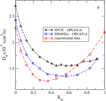
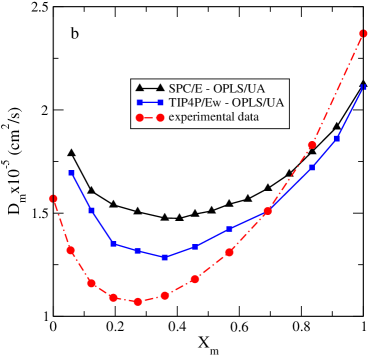
Figure 6: (Color online) Composition dependence of the self-diffusion coefficient of species in water-methanol mixtures from the present simulations in comparison with experimental data [36].

In the two panels of figure 7, the average number of hydrogen bonds per molecule is given as a function of composition for two different geometric definitions of H-bonds. Both definitions lead to similar trends whereas the actual numbers at each composition are a bit different. The values are normalized per the number of molecules of the first species marked next to a given line (w — water; m — methanol). That is, for instance, the line ‘‘w–m’’ gives the number of hydrogen bonds, $\langle n\rangle_{\textrm{HB}}$, for a water molecule that forms connections with methanol ones (normalized by the number of water molecules). In figure 7 (b), the values for the UA and AA models of methanol are also compared: correspondence between the two types of potentials is nearly perfect in this respect. In both panels of figure 7 the vertical dashed line marks an approximate composition ($X_{\textrm{m}}\approx 0.60$) at which the excess mixing volume is at minimum, cf. figure 2 for TIP4P-OPLS-UA combination. The other two water models appear to put the minimum position to about 0.5. The behavior of $\Delta V_{\textrm{mix}}$ is well correlated with the average number of H-bonds. The line ‘‘w–w’’ decays in the entire range of composition reflecting the shrinking of the system due to breaking of H-bonds, whereas the ‘‘w–m’’ line shows an increasing average number of bonds and leading to ‘‘expansion’’ of the system due to an increasing number of bonds. The ‘‘m–m’’ and ‘‘m–w’’ lines exhibit similar trends. Consequently, in two regions where one of the two average numbers of bonds prevail, the excess mixing volume decreases or increases. In the intermediate interval of compositions, where the average numbers of bonds are balanced, $\Delta V_{\textrm{mix}}$ exhibits its minimum. These trends are independent of the definition of the H-bond. If $\Delta V_{\textrm{mix}}$ is in the interval of its minimum value, the self-diffusion coefficients are also approximately around their respective minima. This picture comes from computer simulations of both of the two water models, combined with OPLS/UA methanol; we show only the case of SPC/E to avoid an unnecessary repetition. It is worth mentioning that the excess mixing enthalpy is not straightforward to incorporate into the interpretation of the above data. The reason is that $\Delta H_{\textrm{mix}}$ has ‘‘geometric’’ and energetic terms. Therefore, combining them to interpret the observed trends using a purely geometric definition of H-bonds does not seem to be appropriate.

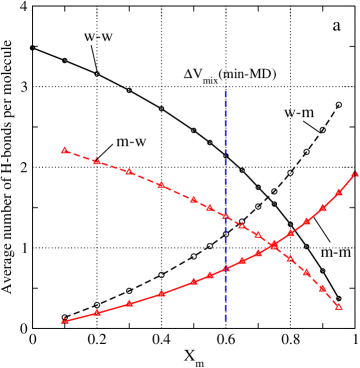
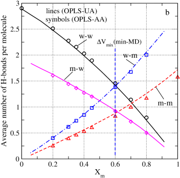
Figure 7: (Color online) Panel (a): The average number of H-bonds per molecule of different species for SPC/E water model combined with united atom modelling of methanol (threshold angle criterion — $30^{\circ}$, see description in the text). Panel (b): Same quantities as in panel (a), with a different geometric criterion for H-bonds between molecules, namely $\theta=150^{\circ}$ as a threshold angle. The OPLS/AA data are given for the sake of comparison. Normalization of the data is explained in the text.

One interesting conjecture coming from the results in figure 7 is that as a general tendency, both water and methanol molecules prefer to coordinate water molecules via H-bonding, similarly to what was found for the mixtures with AA methanol molecules [1]. This can be discerned from the non-linear dependence of the number of H-bonds per molecule on the methanol concentration. In the non-preferential case, the number of both water and methanol H-bonded neighbors would change linearly with concentration. The deviation from linearity is positive for the ‘‘w–w’’ and ‘‘m–w’’ curves, i.e., there are more water molecules hydrogen bonded to both water and methanol molecules than it would be proportional to the composition. By contrast, the deviation is negative for the ‘‘w–m’’ and ‘‘m–m’’ curves, i.e., the number of H-bonded methanol molecules to both water and methanol molecules is smaller than it would be proportional to the methanol concentration. Interestingly, the effect is more pronounced for the less strict definition of H-bonds, as exemplified by figure 7 (a).

By a close inspection of the fractions of methanol and water molecules in different bonding states, as a function of composition (see figure 8), a very similar conclusion may be drawn. These graphs provide the ratio of water or methanol molecules that have a specific number of H-bonded water or methanol neighbors at a given composition. Water can form a maximum of four hydrogen bonds, whereas methanol can form three. If we compare water-water [‘‘w–w’’ in figure 8 (a)] and water-methanol [‘‘w–m’’ in figure 8 (c)] curves, the following observations can be made. As concerns panel (a) of figure 8 that describes the bonding solely within the water subsystem of the mixture, the following trends are worth mentioning. Namely, when the methanol concentration increases (starting from pure water up to pure methanol), the fractions of water molecules with four and three ‘‘w–w’’ bonds monotonously decrease whereas the fraction of molecules that do not participate in bonding substantially grows. Only the fractions of doubly and singly bonded water molecules exhibit maxima at a respective composition, $X_{\textrm{m}}$. In other words, clusters (and branched structures) of exclusively water molecules transform into chains, and thus dimers as well as ‘‘free’’ molecules become abundant. This is a crude description of how a water subsystem of a mixture shrinks. Actually, the minimum value of the excess mixing volume is located in between the two maxima observed for doubly and singly bonded waters.

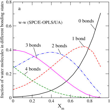
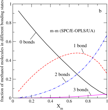
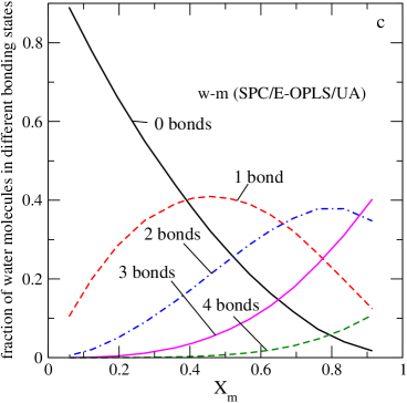
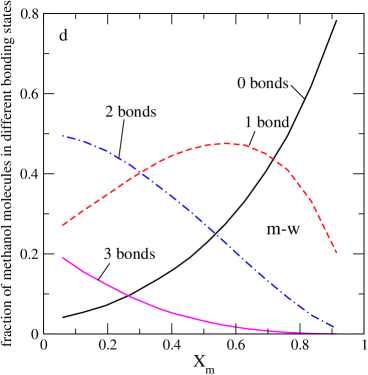
Figure 8: (Color online) A comparison of the fractions of differently bonded molecules of water and methanol for united atom modelling of methanol, panels (a), (b), (c) and (d), respectively. The criterion $\theta=150^{\circ}$ is used.

On the other hand, see figure 8 (c), the fractions describing the bonding of water molecules solely with methanol species exhibit the following trends. The average number of waters initially free of ‘‘w–m’’ bonds rapidly decreases at the expense of the formation of bonded structures. Only the fractions of water molecules with a single bond and double bonds with methanols pass through a maximum value, other fractions with higher number of bonds grow monotonously. Thus, the expansion of the water subsystem occurs via substitution of water molecules by methanols in a shell of neighbors of a given water molecule. In close similarity to what we have seen in panel (a), the minimum of the excess mixing volume occurs at $X_{\textrm{m}}$ located in between two maxima of the curves describing singly and doubly bonded molecules. Similar interpretation can be developed to describe the changes of the bonding within the methanol subsystem and for the changes of the fraction of ‘‘m–w’’ bonds, panels (b) and (d) of figure 8.

Our final focus in the present study is in the relaxation properties of molecules in mixtures. Those certainly are also influenced by H-bonding discussed above. In close similarity to the previous studies [15, 42], we would like to evaluate the reorientational correlation functions determined from

$$C^{\alpha}_{l}(t)=\langle P_{l}[{\bf e}^{\alpha}(t){\cdot}{\bf e}^{\alpha}(0)]\rangle,$$ (5)

where $P_{l}$ is the $l$th order Legendre polynomial and ${\bf e}^{\alpha}$ is the unit vector which points along the $\alpha$ axis in the molecular reference frame. The average is performed over all molecules belonging to a particular species. A typical plot for a mixture of a given composition describing the dependence of the autocorrelation function on time is given in figure 9.

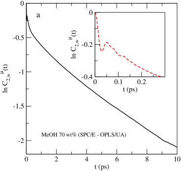
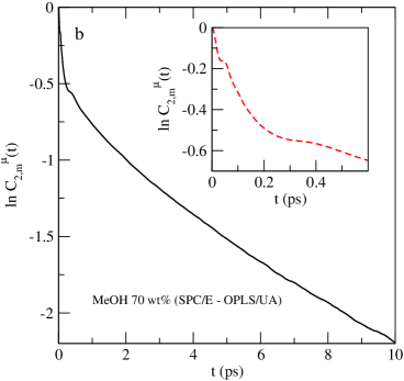
Figure 9: (Color online) An example of the behavior of the orientational auto-correlation functions of the two species in the mixture in the dipole frame. Left-hand panel: water; right-hand panel: methanol.

In the present calculations we used the axis parallel to the molecular dipole moment $\mu$ which is related to dielectric relaxation. Moreover, we calculated $C^{\mu}_{l}$ for $l=2$ for the two species of the mixture. In addition, we performed calculations by using the O–H vector (H is the hydrogen atom belonging to the hydroxyl group of the molecule) as $\alpha$ axis to obtain the corresponding relaxation time. The single-molecule reorientational times follow from integration of the autocorrelation function defined above:

$$\tau^{\alpha}_{l}=\int_{0}^{\infty}\mathrm{d}tC^{\alpha}_{l}(t).$$ (6)

To perform the integration we split the time interval into two pieces, actually it is a commonly accepted procedure [10, 42]. Over a short-time interval, the integration is performed numerically; the upper limit of this interval is chosen between 4 and 5 ns approximately. For a long-time interval, the logarithm of the autocorrelation function is plotted: it behaves as a straight line permitting to analytically evaluate the relevant contribution [42].

Single molecule reorientational times, as calculated for both kinds of the axes mentioned above, are reported in figure 10, as a function of composition. Two trends are qualitatively similar in the behavior of $\tau^{\mu}_{2,i}$ and $\tau^{\textrm{OH}}_{2,i}$ on composition. Namely, both relaxation times characterizing the water species grow with an increasing $X_{\textrm{m}}$, showing a slower dynamics of water molecules in methanol-rich mixtures compared to mixtures with low amount of methanol. On the other hand, the two relaxation times characterizing methanol species in a mixture have maxima, at $X_{\textrm{m}}\approx 0.70$. The slow dynamics, i.e., high relaxation time observed in pure methanol turns even slower at $X_{\textrm{m}}\approx 0.70$; passing this maximum, the relaxation times monotonously drop, showing a faster dynamics of methanol species for mixtures in which the water component is predominant. Such trends are observed for both water models in question when combined with the methanol OPLS/UA model. Very similar trends and a qualitatively similar behavior has been discussed by [15] for $\tau^{\mu}_{2,i}$ on methanol fraction within the framework of TIP4P-OPLS/AA model. Wensink et al. values, however, are substantially lower in comparison with our results with united atom modelling. It is difficult to establish how accurate all these results are due to a lack of well established experimental data. We included some points obtained by Ludwig [43] in figure 10 (b). At present it seems impossible to perform a comprehensive validation of different models versus such kind of experimental data.

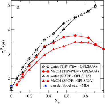
Figure 10: (Color online) The behavior of rotational relaxation times in the dipole frame [panel (a)] and in the OH frame [panel (b)], as a function of the composition of the mixture. The experimental data given as a blue line and stars in panel (b) are from [43].

4 Summary

To summarize this study, we have used molecular dynamics simulations in the NPT ensemble to study some thermodynamic properties, as well as the dynamic and dielectric properties of water-methanol mixtures at room temperature and at ambient pressure in the entire range of their composition. The SPC/E and TIP4P/Ew models combined with the OPLS/UA potential model for methanol are used. This is done as a first step of systematic studies of mixtures of water and a set of alcohols using nonpolarizable models. Our principal findings concern the behavior of density, excess mixing volume and excess mixing enthalpy on composition. Also, we have evaluated the self-diffusion coefficients of both species, reorientational relaxation times and trends of behavior of hydrogen bonding between molecules. Whenever it seemed possible, we looked for a unified interpretation of different properties and performed comparisons with available experimental results. It would be interesting to establish a relation between the structural properties and hydrogen bonding on the one hand and the dielectric constant on the other hand, possibly in the spirit of previous studies of diffusion and power spectra, see e.g., [44]. We would like to note that in our opinion an ample set of properties of the model mixtures in question is required to establish if the modelling is consistent (with experimental data) and successful. A combination of experimental data, computer simulation results and reverse Monte Carlo modelling along the lines developed in [45, 46] may be profitable in this respect. Possible modifications of parameters and combination rules nevertheless should be explored more in detail. At present, it seems that each specific parametrization leads to a successful description of a particular property, such state of art being unsatisfactory. A more sophisticated modelling of alcohols, e.g., OPLS/AA, and the use of possibly more refined water models is necessary to extend the present study and at least make stronger conclusions about various thermodynamic properties of these mixtures. Unfortunately, it seems that some of them are intrinsically impossible to describe very well within the framework of non-polarizable models.

Ukrainian 0

Композицiйна залежнiсть термодинамiчних, динамiчних та дiелектричних властивостей модельних сумiшей вода-метанол. Результати симуляцiй методом молекулярної динамiки

E. Галiцiя-Андрес${}^{\textsf{\footnotesize{\mbox{?}}}}$, Г. Домiнгес${}^{\textsf{\footnotesize{\mbox{?}}}}$, Л. Пустаї${}^{\textsf{\footnotesize{\mbox{?}}}}$, О. Пiзiо${}^{\textsf{\footnotesize{\mbox{?}}}}$

             
${}^{\textsf{\footnotesize 1}}$ Iнститут хiмiї, Нацiональний автономний унiверситет м. Мехiко, Мехiко, Мексика ${}^{\textsf{\footnotesize 2}}$ Iнститут матерiалознавства, Нацiональний автономний унiверситет м. Мехiко, Мехiко, Мексика ${}^{\textsf{\footnotesize 3}}$ Фiзичний дослiдницький центр Вiгнера, Угорська академiя наук, Будапешт, Угорщина

References

- [1] Galicia Andrés E., Pusztai L., Temleitner L., Pizio O., J. Mol. Liq., 2015, 209, 586; doi:10.1016/j.molliq.2015.06.045.
- [2] Berendsen H.J.C., Grigera J.R., Straatsma T.P., J. Phys. Chem., 1987, 91, 6269; doi:10.1021/j100308a038.
- [3] Horn H.W., Swope W.C., Pitera J.W., Madura J.D., Dick T.J., Hura G.L., Head-Gordon T., J. Chem. Phys., 2004, 120, 9665; doi:10.1063/1.1683075.
- [4] Jorgensen W.L., Maxwell D., Tirado-Rives S., J. Am. Chem. Soc., 1996, 118, 11225; doi:10.1021/ja9621760.
- [5] Jorgensen W.L., Madura J.D., J. Am. Chem. Soc., 1983, 105, 1407; doi:10.1021/ja00344a001.
- [6] Okazaki S., Nakanishi K., Touhara H., J. Chem. Phys., 1983, 78, 454; doi:10.1063/1.444525.
- [7] Okazaki S., Touhara H., Nakanishi K., J. Chem. Phys., 1983, 81, 890; doi:10.1063/1.447726.
- [8] Ferrario M., Haughney M., McDonald I.R., Klein M.L., J. Chem. Phys., 1990, 93, 5156; doi:10.1063/1.458652.
- [9] Tanaka H., Gubbins K.E., J. Chem. Phys., 1992, 97, 2626; doi:10.1063/1.463051.
- [10] Laaksonen A., Kusalik P.G., Svishchev I.M., J. Phys. Chem., 1997, 101, 5910; doi:10.1021/jp970673c.
- [11] Palinkas G., Hawlicka E., Heinzinger K., Chem. Phys., 1991, 158, 65; doi:10.1016/0301-0104(91)87055-Z.
- [12] Palinkas G., Bako I., Heinzinger K., Bopp P., Mol. Phys., 1991, 73, 897; doi:10.1080/00268979100101641.
- [13] Palinkas G., Bako I., Z. Naturforsch. A, 1991, 46, 95; doi:10.1515/zna-1991-1-215.
-
[14]
Jorgensen W.L., Chandrasekhar J., Madura J.D., Impey R.W., Klein M.L.,
J. Chem. Phys., 1983, 79, 926;
doi:10.1063/1.445869. -
[15]
Wensink E.J.W., Hoffmann A.C., van Maaren P.J., van der Spoel D.,
J. Chem. Phys., 2003, 119, 7308;
doi:10.1063/1.1607918. - [16] Guevara-Carrion G., Vrabec J., Hasse H., J. Chem. Phys., 2011, 134, 074508; doi:10.1063/1.3515262.
- [17] Abascal J.L., Vega C., J. Chem. Phys., 2005, 123, 234505; doi:10.1063/1.2121687.
- [18] Schnabel T., Srivastava A., Vrabec J., Hasse H., J. Phys. Chem. B, 2007, 111, 9871; doi:10.1021/jp0720338.
- [19] González-Salgado D., Nezbeda I., Fluid Phase Equilib., 2006, 240, 161; doi:10.1016/j.fluid.2005.12.007.
- [20] Moučka F., Nezbeda I., J. Mol. Liq., 2011, 159, 47; doi:10.1016/j.molliq.2010.05.005.
-
[21]
Alejandre J., Chapela G.A., Saint-Martin H., Mendoza N.,
Phys. Chem. Chem. Phys., 2011, 13, 19728;
doi:10.1039/c1cp20858f. - [22] Fuentes-Azcatl R., Alejandre J., J. Phys. Chem. B, 2014, 118, 1263; doi:10.1021/jp410865y.
- [23] Salas F.J., Méndez-Maldonado G.A., Núñez-Rojas E., Aquilar-Pineda G.E., Domínguez H., Alejandre J., J. Chem. Theory Comput., 2015, 11, 683; doi:10.1021/ct500853q.
- [24] Jorgensen W.L., J. Phys. Chem., 1986, 90, 1276; doi:10.1021/j100398a015.
- [25] Van Leeuwen M., Smit B., J. Phys. Chem., 1995, 99, 1831; doi:10.1021/j100007a006.
- [26] Van Leeuwen M.E., Mol. Phys., 1996, 87, 87; doi:10.1080/00268979600100031.
- [27] Veldhuizen R., de Leeuw S.W., J. Chem. Phys., 1996, 105, 2828; doi:10.1063/1.472145.
- [28] Forester T.R., Smith W., DL-POLY Package of Molecular Simulation, CCLRC, Daresbury Laboratory, Daresbury, Warrington, England, 1996.
- [29] Critical Tables of Numerical Data, Phys. Chem and Techn., Washbrun E.W. (Ed.), Knovel, NY, 2003.
- [30] McGlashan M.L., Williamson A.G., J. Chem. Eng. Data, 1976, 21, 196; doi:10.1021/je60069a019.
- [31] Lama R.F., Lu B.C.-Y., J. Chem. Eng. Data, 1965, 10, 216; doi:10.1021/je60026a003.
- [32] Rami Reddy M., Berkowitz M., Chem. Phys. Lett., 1989, 155, 173; doi:10.1016/0009-2614(89)85344-8.
- [33] Gereben O., Pusztai L., Chem. Phys. Lett., 2011, 507, 80; doi:10.1016/j.cplett.2011.02.064.
- [34] Neumann M., Mol. Phys., 1983, 50, 841; doi:10.1080/00268978300102721.
- [35] Albright P.S., Gosting L.J., J. Am. Chem. Soc., 1946, 68, 1061; doi:10.1021/ja01210a043.
-
[36]
Derlacki Z.J., Easteal A.J., Edge A.V.J., Wooolf L.A., Roksandic Z., J. Phys. Chem., 1985, 89, 5318;
doi:10.1021/j100270a039. - [37] Kumar R., Schmidt J.R., Skinner J.L., J. Chem. Phys., 2007, 126, 204107; doi:10.1063/1.2742385.
- [38] Zhang N., Li W., Chen C., Zuo J., Weng L., Mol. Phys., 2013, 111, 939; doi:10.1080/00268976.2012.760050.
- [39] Padró J.A., Saiz L., Guàrdia E., J. Mol. Struct., 1997, 416, 243; doi:10.1016/S0022-2860(97)00038-0.
-
[40]
Guàrdia E., Martí J., Padró J.A., Saiz L., Vanderkooi A.V.,
J. Mol. Liq., 2002, 96–97, 3;
doi:10.1016/S0167-7322(01)00342-7. - [41] Guàrdia E., Martí J., García-Tarrés L., Laria D., J. Mol. Liq., 2005, 117, 63; doi:10.1016/j.molliq.2004.08.004.
- [42] Van der Spoel D., van Maaren P.J., Berendsen H.J.C., J. Chem. Phys., 1998, 108, 10220; doi:10.1063/1.476482.
- [43] Ludwig R., Chem. Phys., 1995, 195, 329; doi:10.1016/0301-0104(95)00050-X.
- [44] Martí J., Padró J.A., Guàrdia E., J. Mol. Liq., 1995, 64, 1; doi:10.1016/0167-7322(95)92817-U.
- [45] Pusztai L., Pizio O., Sokolowski S., J. Chem. Phys., 2008, 129, 184103; doi:10.1063/1.2976578.
- [46] Pusztai L., Harsanyi I., Dominguez H., Pizio O., Chem. Phys. Lett., 2008, 457, 96; doi:10.1016/j.cplett.2008.03.091.
Ukrainian \adddialect\l@ukrainian0 \l@ukrainian