Phonon-like excitations in the two-state Bose-Hubbard model

Abstract

The spectrum of phonon-like collective excitations in the system of Bose-atoms in optical lattice (more generally, in the system of quantum particles described by the Bose-Hubbard model) is investigated. Such excitations appear due to displacements of particles with respect to their local equilibrium positions. The two-level model taking into account the transitions of bosons between the ground state and the first excited state in potential wells, as well as interaction between them, is used. Calculations are performed within the random phase approximation in the hard-core boson limit. It is shown that excitation spectrum in normal phase consists of the one exciton-like band, while in the phase with BE condensate an additional band appears. The positions, spectral weights and widths of bands strongly depend on chemical potential of bosons and temperature. The conditions of stability of a system with respect to the lowering of symmetry and displacement modulation are discussed.

Key words: Bose-Hubbard model, hard-core bosons, Bose-Einstein condensation, excited band, phonons

PACS: 03.75.Hh, 03.75.Lm, 64.70.Tg, 71.35.Lk, 37.10.Jk, 67.85.-d

Abstract

Дослiджується спектр колективних збуджень фононного типу в системi бозе-атомiв у оптичнiй ґратцi (бiльш загально, у системi квантових частинок, якi описуються моделлю Бозе-Хаббарда). Такi збудження виникають завдяки змiщенням частинок вiдносно їх локальних рiвноважних позицiй. Використано дворiвневу модель, яка приймає до уваги переходи бозонiв мiж основним i першим збудженим станом у потенцiальних ямах, а також взаємодiю мiж ними. Розрахунки проведено у наближеннi хаотичних фаз та в границi жорстких бозонiв. Показано, що спектр збуджень складається у нормальнiй фазi з однiєї зони екситонного типу, в той час як у фазi з бозе-конденсатом виникає додаткова зона. Розташування, спектральнi ваги та ширини зон суттєвим чином залежать вiд хiмiчного потенцiалу бозонiв та температури. Обговорюються умови стiйкостi системи вiдносно зниження симетрiї та модуляцiї змiщень.

Ключовi слова: модель Бозе-Хаббарда, жорсткi бозони, бозе-конденсацiя, збуджена зона, фонони

1 Introduction

Bose-Hubbard model (BHM) [1, 2] is a well known model in the solid state physics. In its most applications it is used to describe the thermodynamics and energy spectrum of ultracold bosonic atoms in optical lattices. The main attention was usually paid to phase transition between normal (NO) phase and phase with the Bose-Einstein (BE) condensate [so-called Mott-insulator (MI) — superfluid state (SF) transition] [6, 3, 4, 5]. The model is also intensively used for theoretical description of other phenomena, such as quantum delocalization of hydrogen atoms adsorbed on the surface of transition metal [7, 8], quantum diffusion of light particles on the surface or in the bulk [9, 10], thermodynamics of the impurity ion intercalation into semiconductors [11, 12].

As a general rule, the theoretical consideration is devoted to the behaviour of atoms confined in the lowest vibrational levels in the potential wells of a lattice. However, the study of a quantum delocalization or diffusion reveals an important role of excited vibrational states of particles (ions) in localized positions with a much higher probability of ion hopping between them [9, 13, 14]. In this connection, a possibility of BE condensation in the excited Bloch bands in optical lattices is also considered; in this case, the condition of their sufficient occupation due to the optical pumping (see, e.g., [15]) is imposed. The Bose-Hubbard model was extended to higher vibrational bands and, in the framework of such a generalization, the MI-SF transition to the phase with BE condensate in the pumping-induced quasi-equilibrium state of the system has been described [16]. In the case of orbital degeneracy of the excited state (the p-state, for example) and anisotropy of hopping parameters, the conception of multi-flavour bosons (that correspond to variously polarized bands) was introduced [17]. The possibility of appearance of unconventional p-orbital BE condensate with the non-zero incommensurate wave vector was shown [18, 19]. The double-well lattices open up a new field of researches in this direction [20].

Contrary to that, in the equilibrium case, the BE condensation involving the excited states was not sufficiently studied in the framework of ordinary Bose-Hubbard model. One can mention the systems of spin-1 bosons where the multiplets of local states form the closely-spaced excited levels. It was shown in [21, 22] that MI-SF transition can be of the first order when a single-site spin interaction is of the antiferromagnetic type. A similar effect also takes place for multicomponent Bose system in the optical lattice [23].

A change of the phase transition (PT) order (from the 2nd to the 1st order) is also possible in the equilibrium lattice gas of bosons with the transfer of particles over the excited states. We have considered such a problem in [24, 25, 26] using the Bose-Hubbard model where the only excited nondegenerated state on the lattice site besides the ground state (the so-called two state BHM) was taken into account. The model corresponds to 1D or strongly anisotropic (quasi-1D) optical lattice; it is also close to the situation in a system of light particles (protons, lithium ions) adsorbed on the metal surface.

In the present work we continue the investigation started in [24]. In addition to the analysis of the boson one-particle spectrum performed in [24, 25] we study the collective dynamics of bosons. The pair interaction between particle displacements with respect to their equilibrium positions in the neighbouring wells will be taken into account. In a harmonic case, such displacements are expressed in quantum language in terms of transitions between the nearest vibrational levels. Due to the above mentioned interaction, the collective modes appear; their energy is a function of the wave vector. Attention is paid to changes in the spectrum after the MI-SF transition (both of the 2nd and 1st order) and to the BE condensate appearance. We perform our consideration in the hard-core boson (HCB) limit, which means no more than one particle per site (the single-site problem is here a three-level one). Such a model of hard-core bosons is well known; it is used in a wide range of problems, e.g., local electron pairing mechanism of superconductivity [27], ion transport in ionic conductors [28, 29], BE condensation and related phenomena in optical lattices [30, 31, 32].

2 Model

To consider the phonon-type dynamics in the Bose-atom system in an optical lattice, we use a model which is a simple generalization of the hard-core boson model. Describing vibrational states of Bose-atom in a separate potential well in the lattice, we take into account the first excited level besides the ground one. Let us suppose that this level is nondegenerate; such a situation can be realized in the case of low local symmetry. At the same time, we impose a usual (for hard-core bosons) restriction: no more than one particle per lattice site. The model of this type was used by us while investigating the conditions, at which the Bose-Einstein (BE) condensate appears when the particles are hopping only over the excited states. Hamiltonian of the model was written as follows:

$$\hat{H} =\sum_{ij}t(i,j)b_{i}^{+}b_{j}+{\sum}_{ij}t^{\prime}(i,j)c_{i}^{+}c_{j}+\sum_{ij}t^{\prime\prime}(i,j)(b_{i}^{+}c_{j}+c_{i}^{+}b_{j})$$

$$\quad+\sum_{i}(\varepsilon-\mu)b_{i}^{+}b_{i}+\sum_{i}(\varepsilon^{\prime}-\mu)c_{i}^{+}c_{i},$$ (2.1)

where $b_{i}$ and $b_{i}^{+}$ ($c_{i}$ and $c_{i}^{+}$) are Bose operators of annihilation and creation of particles in the ground (excited) states; $\varepsilon$ and $\varepsilon^{\prime}$ are respective energies of states ($\delta=\varepsilon^{\prime}-\varepsilon$ is the on-site excitation energy); $\mu$ is the boson chemical potential. For matrix elements describing the particle hoppings onto the neighbouring sites we take [24]

$$t(i,j)=0,\qquad t^{\prime\prime}(i,j)=0,\qquad t^{\prime}(i,j)\neq 0$$ (2.2)

basing on the above mentioned arguments. It should be also noted that such an approximation agrees with the results of numerical estimates for optical lattice performed by T. Müller (see [33]), where it was shown that the tunneling matrix elements $t$ and $t^{\prime}$ can significantly differ by up to one order (or even more) of magnitude.

Introducing the Hubbard operators $X_{i}^{n,m;n^{\prime}m^{\prime}}\equiv|i,n,m\rangle\langle i,n^{\prime},m^{\prime}|$, acting on a single-site basis $|n_{i}^{b},n_{i}^{c}\rangle\equiv|i,n_{i}^{b},n_{i}^{c}\rangle$ (which is formed by particle occupation numbers in the ground and in the excited states), we can write

$$b_{i}=\sum_{n_{b}=0}^{\infty}\sum_{n_{c}=0}^{\infty}\sqrt{n_{b}+1}X_{i}^{n_{b},n_{c};n_{b+1},n_{c}},\qquad c_{i}=\sum_{n_{b}=0}^{\infty}\sum_{n_{c}=0}^{\infty}\sqrt{n_{c}+1}X_{i}^{n_{b},n_{c};n_{b},n_{c+1}}.$$ (2.3)

After transition to the hard-core boson limit, there remain only the $|0,0\rangle$, $|1,0\rangle$ and $|0,1\rangle$ states. In this case the relations (2.3) take the following form:

$$b_{i}=X_{i}^{00;10},\qquad c_{i}=X_{i}^{00;01}.$$ (2.4)

Respectively,

$$b_{i}^{+}=X_{i}^{10;00},\qquad c_{i}^{+}=X_{i}^{01;00}.$$ (2.5)

In what follows, we use the shortened notations

$$|0,0\rangle=|0\rangle,\qquad|1,0\rangle=|1\rangle,\qquad|0,1\rangle=|2\rangle.$$ (2.6)

In such a case,

$$b_{i}=X_{i}^{01},\qquad b_{i}^{+}=X_{i}^{10};\qquad c_{i}=X_{i}^{02},\qquad c_{i}^{+}=X_{i}^{20}.$$ (2.7)

When particles are moving through the lattice only in the excited state, BE condensate is described by the order parameter $\langle c_{i}\rangle=\langle c_{i}^{+}\rangle=\xi$ (or $\langle X_{i}^{02}\rangle=\langle X_{i}^{20}\rangle=\xi$). With the help of identity

$$c_{i}^{+}c_{j}=(c_{i}^{+}+c_{j})\xi+(c_{i}^{+}-\xi)(c_{j}-\xi)-\xi^{2}.$$

Hamiltonian (2.1) can be presented as follows:

$$\hat{H}=\hat{H}_{0}+\sum_{ij}t^{\prime}(i,j)(c_{i}^{+}-\xi)(c_{j}-\xi)+N\lvert t^{\prime}_{0}\rvert\xi^{2},$$ (2.8)

where the first term $\hat{H}_{0}$ is the mean-field Hamiltonian

$$\hat{H}_{0}=-\lvert t^{\prime}_{0}\rvert\xi\sum_{i}(c_{i}^{+}+c_{i})+\sum_{i}(\varepsilon-\mu)b_{i}^{+}b_{i}+\sum_{i}(\varepsilon^{\prime}-\mu)c_{i}^{+}c_{i}+N\lvert t^{\prime}_{0}\rvert\xi^{2}.$$ (2.9)

Here, the notation $\sum_{j}t^{\prime}(i,j)=t^{\prime}_{0}=-\lvert t^{\prime}_{0}\rvert$ is used; $t^{\prime}_{0}\equiv t^{\prime}_{\vec{q}=0}$ is the zero-momentum Fourier-transform of the hopping matrix element. We consider the case, when $t^{\prime}(i,j)<0$ [24].

In terms of $X$-operators acting on the three-state basis (2.6)

$$\hat{H}_{0}=\sum_{i}\hat{H}_{i},\qquad\hat{H}_{i}=(\varepsilon-\mu)X_{i}^{11}+(\varepsilon{{}^{\prime}}-\mu)X_{i}^{22}-\lvert t^{\prime}_{0}\rvert\xi(X_{i}^{02}+X_{i}^{20})+\lvert t^{\prime}_{0}\rvert\xi^{2}.$$ (2.10)

The single-site Hamiltonian $\hat{H}_{i}$ is diagonalized by transformation

$$|0\rangle =\cos\alpha\cdot|\tilde{0}\rangle-\sin\alpha\cdot|\tilde{2}\rangle,$$

$$|1\rangle =|\tilde{1}\rangle,$$

$$|2\rangle =\cos\alpha\cdot|\tilde{2}\rangle+\sin\alpha\cdot|\tilde{0}\rangle,$$ (2.11)

where

$$\cos 2\alpha=\frac{\varepsilon^{\prime}-\mu}{\sqrt{(\varepsilon^{\prime}-\mu)^{2}+4\xi^{2}t_{0}^{\prime 2}}},\qquad\sin 2\alpha=\frac{2\xi\lvert t^{\prime}_{0}\rvert}{\sqrt{(\varepsilon^{\prime}-\mu)^{2}}+4\xi^{2}t_{0}^{\prime 2}}.$$ (2.12)

As a result,

$$\hat{H}_{i}=\tilde{\lambda}_{0}\tilde{X}_{i}^{00}+\tilde{\lambda}_{1}\tilde{X}_{i}^{11}+\tilde{\lambda}_{2}\tilde{X}_{i}^{22}+\lvert t^{\prime}_{0}\rvert\xi^{2},$$ (2.13)

here, the $\tilde{X}_{i}^{mm}$ operators act on ‘‘tilded’’ basis, and the energy eigenvalues are as follows:

$$\tilde{\lambda}_{0,2}=\frac{\varepsilon^{\prime}-\mu}{2}\mp\frac{1}{2}\sqrt{(\varepsilon^{\prime}-\mu)^{2}+4\xi^{2}t_{0}^{{}^{\prime}2}},\qquad\tilde{\lambda}_{1}=\varepsilon-\mu.$$ (2.14)

We intend to investigate the spectrum of phonon-type excitations, which are connected with displacements of Bose-particles from their equilibrium positions in the sites of optical lattice. In the quantum description, the operators $\tilde{X}_{i}$ of such displacements are characterized by their matrix elements. The latter are nonzero when calculated between the states having different parity (it is assumed usually that local potential wells are harmonic and, correspondingly, the oscillatory wave functions form a basis of local states). In the case when only one excited state is taken into account, only matrix elements $\langle 0|\hat{x}|1\rangle$ and $\langle 1|\hat{x}|0\rangle$ are of current interest. In the second quantization representation

$$\hat{x}_{i}=d(c_{i}^{+}b_{i}+b_{i}^{+}c_{i})=d\left(X_{i}^{21}+X_{i}^{12}\right),$$ (2.15)

here, $d=\langle 0|\hat{x}|1\rangle=\langle 1|\hat{x}|0\rangle$

Collective vibrations arise due to interaction between particle displacements. Let us write it in the following form:

$$\hat{H}^{\prime}=\frac{1}{2}\sum_{ij}\Phi(i,j)\hat{x}_{i}\hat{x}_{j}.$$ (2.16)

As distinct from direct interparticle interaction (that looks like $~{}V(i,j)n_{i}n_{j}$), the interaction (2.16) has another nature; it is caused by transitions between the ground and excited states. This interaction can be considered as an analogue of the so-called resonant interaction that is responsible for the dynamics of excitations (Frenkel excitons) in molecular crystals.

In terms of ‘‘tilded’’ operators

$$b_{i} =\cos\alpha\cdot\tilde{X}_{i}^{01}-\sin\alpha\cdot\tilde{X}_{i}^{21},$$

$$c_{i} =\sin\alpha\cos\alpha\cdot\left(\tilde{X}_{i}^{00}-\tilde{X}_{i}^{22}\right)+\cos^{2}\alpha\cdot\tilde{X}_{i}^{02}-\sin^{2}\alpha\cdot\tilde{X}_{i}^{20},$$ (2.17)

and

$$\hat{x}_{i}=d\sin\alpha\cdot\left(\tilde{X}_{i}^{10}+\tilde{X}_{i}^{01}\right)+d\cos\alpha\cdot\left(\tilde{X}_{i}^{12}+\tilde{X}_{i}^{21}\right).$$ (2.18)

We now use the technique of the Zubarev two-time temperature Green’s functions to study the vibrational spectrum. Let us introduce the commutator Green’s function of displacements

$$\langle\langle\hat{x}_{i}|\hat{x}_{j}\rangle\rangle=d^{2}\langle\langle(c_{i}^{+}b_{i}+b_{i}^{+}c_{i}|(c_{j}^{+}b_{j}+b_{j}^{+}c_{j})\rangle\rangle.$$ (2.19)

Using (2.18), this function can be presented as linear combination of functions defined on $\tilde{X}$-operators

$$\langle\langle\hat{x}_{i}|\hat{x}_{j}\rangle\rangle =d^{2}\left[\sin^{2}\alpha\left(G_{ij}^{10,10}+G_{ij}^{01,10}+G_{ij}^{10,01}+G_{ij}^{01,01}\right)\right.$$

$$\quad+\cos^{2}\alpha\left(G_{ij}^{12,12}+G_{ij}^{21,12}+G_{ij}^{12,21}+G_{ij}^{21,21}\right)$$

$$\quad+\sin\alpha\cos\alpha\left(G_{ij}^{12,10}+G_{ij}^{21,10}+G_{ij}^{12,01}+G_{ij}^{21,01}\right.$$

$$\left.\!\left.\!\quad{}+G_{ij}^{10,12}+G_{ij}^{01,12}+G_{ij}^{10,21}+G_{ij}^{01,21}\right)\right],$$ (2.20)

where

$$G_{ij}^{pq,rs}=\langle\langle\tilde{X}_{i}^{pq}|\tilde{X}_{j}^{rs}\rangle\rangle.$$ (2.21)

The poles of function (2.18) determine the energies of collective vibrations while the imaginary part $\operatorname{Im}\langle\langle\hat{x}_{i}|\hat{x}_{j}\rangle\rangle_{\omega+\mathrm{i}\varepsilon}$ is connected with spectral density

$$\rho(\omega)=-\frac{2}{\hbar}\operatorname{Im}\langle\langle\tilde{x}_{i}|\tilde{x}_{i}\rangle\rangle_{\omega+\mathrm{i}\varepsilon}$$ (2.22)

which provides a more complete description of the vibrational spectrum, providing in particular information on the statistical weights of boson vibrational modes.

3 Green’s function of displacements

We calculate the Green’s function (2.21) in the random phase approximation (RPA) using the Hamiltonian

$$\tilde{H}=\sum_{i}\hat{H}_{i}+\hat{H}^{\prime},$$ (3.1)

where we add the pair interaction between the particle displacements to the mean-field Hamiltonian. Let us employ a standard scheme of the equation of motion method. Accordingly, in the frequency representation, the following equation

$$\hbar\omega\langle\langle\tilde{X}_{i}^{pq}|\tilde{X}_{j}^{rs}\rangle\rangle=\frac{\hbar}{2\pi}\delta_{ij}\langle\tilde{X}^{ps}\delta_{qr}-\tilde{X}^{rq}\delta_{sp}\rangle+\langle\langle[\tilde{X}_{i}^{pq},\tilde{H}]|\tilde{X}_{j}^{rs}\rangle\rangle$$ (3.2)

for Green’s function (2.21) is used.

Equation of motion for separate operator $\tilde{X}_{i}^{pq}$ can be easily written taking into account the commutation relations for $\tilde{X}$-operators. In particular, for $\tilde{X}^{1r}_{l}$ operator, we have

$$[\tilde{X}_{l}^{12},\hat{H}] =\left[(\varepsilon^{\prime}-\mu)\cos^{2}\alpha-(\varepsilon-\mu)\right]\tilde{X}_{l}^{12}+(\varepsilon^{\prime}-\mu)\sin\alpha\cos\alpha\tilde{X}_{l}^{10}$$

$$\quad+\sum_{j}t^{\prime}(l,j)\left(\cos^{2}\alpha\tilde{X}_{l}^{10}-\sin\alpha\cos\alpha\tilde{X}_{l}^{12}\right)c_{j}$$

$$\quad-\sum_{i}t^{\prime}(i,l)c_{i}^{+}\left(\sin^{2}\alpha\tilde{X}_{l}^{10}+\sin\alpha\cos\alpha\tilde{X}_{l}^{12}\right)$$

$$\quad+\sum_{j}\Phi(l,j)\cos\alpha\left(\tilde{X}_{l}^{11}-\tilde{X}_{l}^{22}\right)\hat{x}_{j}d.$$ (3.3)

In the spirit of RPA scheme, we decouple the pair products of operators taking into account that mean values of nondiagonal $\tilde{X}$-operators are equal to zero in the applied approximation

$$\tilde{X}_{l}^{10}c_{j}\approx\langle\tilde{X}_{l}^{10}\rangle c_{j}+\tilde{X}_{l}^{10}\langle c_{j}\rangle-\langle\tilde{X}_{l}^{10}\rangle\langle c_{j}\rangle=\tilde{X}_{l}^{10}\langle c_{j}\rangle,$$ (3.4)

and, similarly,

$$\tilde{X}_{l}^{12}c_{j}\approx\tilde{X}_{l}^{12}\langle c_{j}\rangle,\qquad c_{i}^{+}\tilde{X}_{l}^{10}\approx\langle c_{i}^{+}\rangle\tilde{X}_{l}^{10},\qquad c_{i}^{+}\tilde{X}_{l}^{12}\approx\langle{c}_{i}^{+}\rangle\tilde{X}_{l}^{10}.$$

At the same time,

$$\left(\tilde{X}_{l}^{11}-\tilde{X}_{l}^{22}\right)\tilde{x}_{j} =\left(\tilde{X}_{l}^{11}-\tilde{X}_{l}^{22}\right)d\left[\sin\alpha\left(\tilde{X}_{j}^{10}+\tilde{X}_{j}^{01}\right)+\cos\alpha\left(\tilde{X}_{j}^{12}+\tilde{X}_{j}^{21}\right)\right]$$

$$\approx\langle\tilde{X}_{l}^{11}-\tilde{X}_{l}^{22}\rangle\hat{x}_{j}.$$ (3.5)

Here,

$$\langle c_{j}\rangle=\sin\alpha\cos\alpha\cdot Q,\qquad\langle c_{i}^{+}\rangle=\sin\alpha\cos\alpha\cdot Q,\qquad\langle\tilde{X}_{l}^{11}-\tilde{X}_{l}^{22}\rangle=-\sigma,$$ (3.6)

where

$$Q=\langle\tilde{X}^{00}-\tilde{X}^{22}\rangle,\qquad\sigma=\langle\tilde{X}^{22}-\tilde{X}^{11}\rangle$$ (3.7)

(here we consider the uniform case).

As a result,

$$[\tilde{X}_{l}^{12},\hat{H}]=\Delta_{21}\tilde{X}_{l}^{12}+\Delta^{\prime}\tilde{X}_{l}^{10}-\sigma d^{2}\cos\alpha\sum_{j}\Phi(l,j)\left[\sin\alpha\left(\tilde{X}_{j}^{10}+\tilde{X}_{j}^{01}\right)+\cos\alpha\left(\tilde{X}_{j}^{12}+\tilde{X}_{j}^{21}\right)\right].$$ (3.8)

Here,

$$\Delta_{21} =(\varepsilon^{\prime}-\mu)\cos^{2}\alpha-(\varepsilon-\mu)+\frac{1}{2}\sin^{2}2\alpha\cdot Q\cdot\lvert t^{\prime}_{0}\rvert\equiv\tilde{\lambda}_{2}-\tilde{\lambda}_{1},$$

$$\Delta^{\prime} =(\varepsilon^{\prime}-\mu)\sin\alpha\cos\alpha-\frac{1}{2}\sin 2\alpha\cos 2\alpha\cdot Q\cdot\lvert t^{\prime}_{0}\rvert=0.$$ (3.9)

In a similar way, we can come to the equation of motion for the $\tilde{X}_{l}^{10}$ operator

$$[\tilde{X}_{l}^{10},\hat{H}]=\Delta_{01}\tilde{X}_{l}^{10}+\Delta^{\prime}\tilde{X}_{l}^{12}-Q^{\prime}d\sin\alpha\sum_{j}\Phi(l,j)\left[\sin\alpha\left(\tilde{X}_{j}^{10}+\tilde{X}_{j}^{01}\right)+\cos\alpha\left(\tilde{X}_{j}^{12}+\tilde{X}_{j}^{21}\right)\right],$$ (3.10)

where

$$\Delta_{01}=(\varepsilon^{\prime}-\mu)\sin^{2}\alpha-(\varepsilon-\mu)-\frac{1}{2}\sin^{2}2\alpha\cdot Q\cdot\lvert t^{\prime}_{0}\rvert\equiv\tilde{\lambda}_{0}-\tilde{\lambda}_{1}.$$ (3.11)

Equations of motion for $\tilde{X}_{l}^{21}$ and $\tilde{X}_{l}^{10}$ operator can be found from (3.8) and (3.10) with the help of relations

$$[\tilde{X}_{l}^{21},\hat{H}]=-[\tilde{X}_{l}^{12},\hat{H}]^{+},\qquad[\tilde{X}_{l}^{01},\hat{H}]=[\tilde{X}_{l}^{10},\hat{H}]^{+}.$$ (3.12)

Using the formulae (3.8), (3.10) and (3.12), one can write a set of equations (3.2) in the explicit form. In a matrix representation, after the Fourier transition to wave vectors, it has the following form:

$$\|\hat{W}\|\times\left(\begin{array}[]{c}G^{12,rs}\\ G^{10,rs}\\ G^{21,rs}\\ G^{01,rs}\end{array}\right)=\|\hat{I}\|^{rs},$$ (3.17)

where

$$\|\hat{W}\|=\left(\begin{array}[]{cccc}\hbar\omega-\Delta_{21}+\sigma A_{q}&\sigma C_{q}&\sigma A_{q}&\sigma C_{q}\\ Q^{\prime}C_{q}&\hbar\omega-\Delta_{01}+Q^{\prime}B_{q}&Q^{\prime}C_{q}&Q^{\prime}B_{q}\\ -\sigma A_{q}&-\sigma C_{q}&\hbar\omega+\Delta_{21}-\sigma A_{q}&-\sigma C_{q}\\ -Q^{\prime}C_{q}&-Q^{\prime}B_{q}&-Q^{\prime}C_{q}&\hbar\omega+\Delta_{01}-Q^{\prime}B_{q}\end{array}\right),$$ (3.22)

and

$$\|\hat{I}\|^{21}=-\frac{\hbar}{2\pi}\left(\begin{array}[]{c}\sigma\\ 0\\ 0\\ 0\end{array}\right),\quad\|\hat{I}\|^{01}=\frac{\hbar}{2\pi}\left(\begin{array}[]{c}0\\ Q^{\prime}\\ 0\\ 0\end{array}\right),\quad\|\hat{I}\|^{12}=\frac{\hbar}{2\pi}\left(\begin{array}[]{c}0\\ 0\\ \sigma\\ 0\end{array}\right),\quad\|\hat{I}\|^{10}=\frac{\hbar}{2\pi}\left(\begin{array}[]{c}0\\ 0\\ 0\\ Q^{\prime}\end{array}\right).$$ (3.23)

Here, the notations are introduced

$$A_{q}=d^{2}\Phi_{q}\cos^{2}\alpha,\qquad B_{q}=d^{2}\Phi_{q}\sin^{2}\alpha,\qquad C_{q}=d^{2}\Phi_{q}\sin\alpha\cos\alpha;$$ (3.24)

moreover,

$$Q^{\prime}=\langle\tilde{X}^{00}-\tilde{X}^{11}\rangle\equiv Q+\sigma.$$ (3.25)

The function $\Phi_{q}$ is the Fourier-transform of the pair interaction of displacements.

$$\Phi_{q}=\sum_{ij}{\mathrm{e}}^{\mathrm{i}\vec{q}(\vec{R}_{i}-\vec{R}_{j})}\Phi(i,j).$$

A set of equations (3.17) decomposes into independent subsets; each of them consists of four equations. Their solutions can be easily found. After substitution into formula (2.20) and after some simplifications, we get

$$\langle\langle\hat{x}|\hat{x}\rangle\rangle_{\omega,\vec{q}} =-\frac{\hbar}{2\pi}\frac{d^{2}}{D(\omega)}\left[2\Delta_{01}\sin^{2}\alpha\cdot Q^{\prime}(\hbar^{2}\omega^{2}-\Delta_{21}^{2})\right.$$

$$\left.\quad+2\Delta_{21}\cos^{2}\alpha\cdot\sigma(\hbar^{2}\omega^{2}-\Delta_{01}^{2})\right].$$ (3.26)

Denominator $D(\omega)$ is given by an expression

$$D(\omega) =(\hbar^{2}\omega^{2}-\Delta_{21}^{2})(\hbar^{2}\omega^{2}-\Delta_{01}^{2})+2\sigma A_{q}\Delta_{21}(\hbar^{2}\omega^{2}-\Delta_{01}^{2})$$

$$\quad+2Q^{\prime}B_{q}\Delta_{01}(\hbar^{2}\omega^{2}-\Delta_{21}^{2}).$$ (3.27)

Its zeros determine the poles of the Green’s function. Consequently, having solved the equation

$$D(\omega)=0,$$ (3.28)

we can calculate the vibrational spectrum of Bose-particles.

The solutions of equation (3.28) are as follows:

$$\hbar\omega_{1,2}\equiv\varepsilon_{1,2}=\pm\sqrt{y_{1}},\qquad\hbar\omega_{3,4}\equiv\varepsilon_{3,4}=\pm\sqrt{y_{2}},$$ (3.29)

where

$$y_{1,2} =\frac{1}{2}\left(\Delta_{21}^{2}+\Delta_{01}^{2}-2\Delta_{01}Q^{\prime}B_{q}-2\Delta_{21}\sigma A_{q}\right)$$

$$\quad\pm\left[\frac{1}{4}\left(\Delta_{21}^{2}-\Delta_{01}^{2}+2\Delta_{01}Q^{\prime}B_{q}-2\Delta_{21}\sigma A_{q}\right)^{2}+4\Delta_{01}\Delta_{21}Q^{\prime}B_{q}\sigma A_{q}\right].$$ (3.30)

In general, there are four branches in spectrum. They form two pairs which differ by sign among themselves. Their dispersion laws are determined by the dependence of $A_{q}$, $B_{q}$, and $C_{q}$ functions (which are linear in the $\Phi_{q}$ interaction) upon the wave vector.

Band edges of the $\varepsilon_{1\ldots{4}}(\vec{q})$ branches can be obtained putting $d^{2}\Phi_{q}=\pm W$ (a 2W parameter determines the interval of the change of the Fourier-transform $\Phi_{q}$ within the 1st Brillouin zone). Depending on the boson chemical potential value, the excitation spectrum (3.29) changes its form both in the range of NO or SF phase and at the transition between them. This is illustrated in figures 1 and 2 where the position of band edges as function of $\mu$ at various temperatures is shown (for the sake of simplicity we present only positive branches of the spectrum).

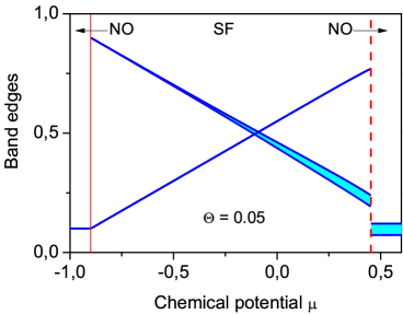
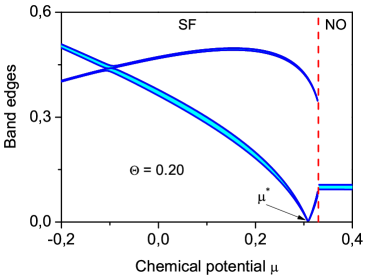
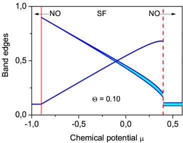
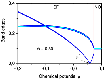
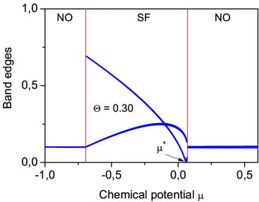
Figure 1: (Color online) Excitation energy bands as functions of boson chemical potential at various temperatures ($\Theta=k_{\mathrm{B}}T$). Parameter values: $\delta=0.1$, $W=0.03$. Here and in figures 2–5 energetic quantities are given in units of $\lvert t^{\prime}_{0}\rvert$; thin solid (dotted) vertical lines correspond to 1st (2nd) order PT.

In normal phase (when BE-condensate is absent) $\alpha=0$, $B_{q}=C_{q}=0$, the expression (3.26) for the Green’s function greatly simplifies

$$\langle\langle\hat{x}|\hat{x}\rangle\rangle_{\omega,\vec{q}}^{\text{(NO)}}=-\frac{\hbar}{2\pi}d^{2}\frac{2\Delta_{21}\sigma}{\hbar^{2}\omega^{2}-\Delta^{2}_{21}+2\sigma d^{2}\Phi_{q}\Delta_{21}}.$$ (3.31)

Here, two branches remain, whose energies are equal in modulus but differ among themselves by sign.

$$\varepsilon_{1,2}^{\text{(NO)}}=\pm\left[\Delta_{21}^{2}-2\sigma d^{2}\Phi_{q}\Delta_{21}\right]^{1/2}.$$ (3.32)

Among the branches existing in the SF phase spectrum, two branches ($\varepsilon_{1}$ and $\varepsilon_{2}$) transform into branches $\varepsilon_{1}^{\text{(NO)}}$ and $\varepsilon_{2}^{\text{(NO)}}$ at the phase transition to the NO phase. The other two ($\varepsilon_{3}$ and $\varepsilon_{4}$) are new ones; they appear in the SF phase due to the presence of the BE condensate. This can be seen while applying the expansion in power series of the rotation angle $\alpha$ [see expressions (2.11) and (2.12)] at small values of the order parameter $\xi$ (near the border of the SF phase region in the case of SF-NO transition of the second order). In this case we obtain:

$$\varepsilon_{1,2}^{2} =\Delta_{21}^{2}-2\sigma\Delta_{21}d^{2}\Phi_{q}(1-\alpha^{2})+\frac{4Q^{\prime}\sigma\Delta_{01}\Delta_{21}d^{4}\Phi_{q}^{2}}{\Delta_{21}^{2}-\Delta_{01}^{2}-2\sigma\Delta_{21}d^{2}\Phi_{q}}\alpha^{2},$$

$$\varepsilon_{3,4}^{2} =\Delta_{01}^{2}+\frac{2Q^{\prime}\Delta_{01}(\Delta_{01}^{2}-\Delta_{21}^{2})d^{2}\Phi_{q}}{\Delta_{21}^{2}-\Delta_{01}^{2}-2\sigma\Delta_{21}d^{2}\Phi_{q}}\alpha^{2}.$$ (3.33)

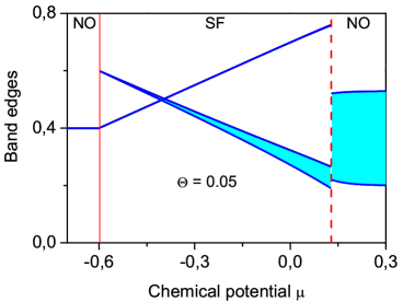
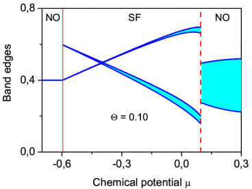
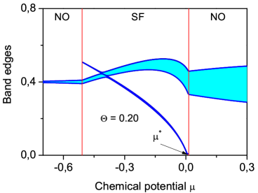
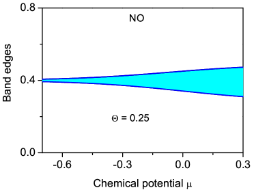
Figure 2: (Color online) Excitation energy bands as functions of boson chemical potential at various temperatures. Parameter values: $\delta=0.4$, $W=0.15$.

At a small $\Phi_{q}$ interaction, when the linear approximation can be used,

$$\varepsilon_{1,2}=\pm\left[\Delta_{21}-\sigma d^{2}\Phi_{q}(1-\alpha^{2})\right],\qquad\varepsilon_{3,4}=\pm\left[\Delta_{01}-Q^{\prime}d^{2}\Phi_{q}\alpha^{2}\right].$$ (3.34)

One can see that $\varepsilon_{1,2}\rightarrow\varepsilon_{1,2}^{\text{(NO)}}$, $\varepsilon_{3,4}\rightarrow\pm\Delta_{01}$ at $\alpha\rightarrow 0$. When passing more deeply into SF phase, when $\xi$ parameter (angle $\alpha$) increases, the widths of bands that correspond to the branches of spectrum are changed. The bands $\varepsilon_{3}$ and $\varepsilon_{4}$ become broader while the bands $\varepsilon_{1}$ and $\varepsilon_{2}$ become narrower (see figures 1 and 2). At the point of the 1st order phase transition (see the phase diagram, figure 3), the positions of bands are changed abruptly while in the case of the 2nd order PT, such a change is continuous. As a whole, the weights of the bands diminish when chemical potential $\mu$ decreases and passes from a positive region to a negative one. Besides that, the redistribution of their statistical weights takes place. The effect can be described by means of the corresponding spectral densities. One can calculate the latter using the Green’s function $\langle\langle\hat{x}|\hat{x}\rangle\rangle$.

Starting from (3.26) we can write the Green’s function $\langle\langle\hat{x}|\hat{x}\rangle\rangle$ in the following form:

$$\langle\langle\hat{x}|\hat{x}\rangle\rangle_{\omega,q}=-\frac{\hbar}{2\pi}d^{2}\frac{Q(\hbar\omega)}{(\hbar^{2}\omega^{2}-y_{1})(\hbar^{2}\omega^{2}-y_{2})},$$ (3.35)

where

$$Q(\hbar\omega)=2\Delta_{01}\sin^{2}\alpha Q^{\prime}\left(\hbar^{2}\omega^{2}-\Delta_{21}^{2}\right)+2\Delta_{21}\cos^{2}\alpha\sigma\left(\hbar^{2}\omega^{2}-\Delta_{01}^{2}\right).$$ (3.36)

After decomposition into simple fractions

$$\langle\langle\hat{x}|\hat{x}\rangle\rangle_{\vec{q},\omega} =-\frac{\hbar}{2\pi}d^{2}\left[\frac{1}{\hbar\omega-\sqrt{y_{1}}}\;\frac{Q(\sqrt{y_{1}})}{2\sqrt{y_{1}}(y_{1}-y_{2})}-\frac{1}{\hbar\omega+\sqrt{y_{1}}}\;\frac{Q(-\sqrt{y_{1}})}{2\sqrt{y_{1}}(y_{1}-y_{2})}\right.$$

$$\left.\!\quad{}+\frac{1}{\hbar\omega-\sqrt{y_{2}}}\;\frac{Q(\sqrt{y_{2}})}{2\sqrt{y_{2}}(y_{2}-y_{1})}-\frac{1}{\hbar\omega+\sqrt{y_{2}}}\;\frac{Q(-\sqrt{y_{2}})}{2\sqrt{y_{2}}(y_{2}-y_{1})}\right].$$ (3.37)

Since $Q(\sqrt{y_{i}})=Q(-\sqrt{y_{i}})$, the formula (3.37) can be written as follows:

$$\langle\langle\hat{x}|\hat{x}\rangle\rangle_{\vec{q},\omega} =-\frac{1}{2\pi}\frac{d^{2}}{2}\frac{1}{\varepsilon_{1}^{2}-\varepsilon_{3}^{2}}\left[\frac{Q(\varepsilon_{1})}{\varepsilon_{1}}\left(\frac{1}{\omega-\varepsilon_{1}/\hbar}-\frac{1}{\omega-\varepsilon_{2}/\hbar}\right)\right.$$

$$\left.\!\quad{}-\frac{Q(\varepsilon_{3})}{\varepsilon_{3}}\left(\frac{1}{\omega-\varepsilon_{3}/\hbar}-\frac{1}{\omega-\varepsilon_{4}/\hbar}\right)\right].$$ (3.38)

Spectral density calculated per lattice site is given by the relation:

$$\rho(\omega)=\frac{1}{N}\sum_{q}\rho_{q}(\omega),$$ (3.39)

where

$$\rho_{q}(w)=-2\operatorname{Im}\langle\langle\hat{x}|\hat{x}\rangle\rangle_{\vec{q},\omega+\mathrm{i}\varepsilon}.$$ (3.40)

It is easy to determine the imaginary part of the function (3.38); then

$$\rho_{q}(\omega) =-\frac{d^{2}}{2(\varepsilon_{1}^{2}-\varepsilon_{3}^{2})}\left\{\frac{Q(\varepsilon_{1})}{\varepsilon_{1}}\left[\delta(\omega-\varepsilon_{1}/\hbar)-\delta(\omega-\varepsilon_{2}/\hbar)\right]\right.$$

$$\left.\!\quad{}-\frac{Q(\varepsilon_{3})}{\varepsilon_{3}}\left[\delta(\omega-\varepsilon_{3}/\hbar)-\delta(\omega-\varepsilon_{4}/\hbar)\right]\right\}.$$ (3.41)

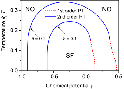
Figure 3: (Color online) Mean-field phase diagram of the two-state Bose-Hubbard model [24].

In the case of normal phase, the expression (3.41) for function $\rho_{q}(\omega)$ is more simple. Here, at $\alpha=0$,

$$Q(\hbar\omega)=2\Delta_{21}\sigma(\hbar^{2}\omega^{2}-\Delta_{01}^{2}),$$ (3.42)

and, respectively,

$$Q(\varepsilon_{1})=2\Delta_{21}\sigma([\varepsilon_{1}^{\text{(NO)}}]^{2}-\Delta_{01}^{2}),\qquad Q(\varepsilon_{3})=0.$$ (3.43)

Thus, we have

$$\rho_{q}^{(N_{0})}(\omega)=-d^{2}\frac{\Delta_{21}\sigma}{\varepsilon_{1}^{\text{(NO)}}(q)}\left[\delta\left(\omega-\frac{\varepsilon_{1}^{\text{(NO)}}(q)}{\hbar}\right)-\delta\left(\omega-\frac{\varepsilon_{2}^{\text{(NO)}}(q)}{\hbar}\right)\right].$$ (3.44)

The energies $\varepsilon_{1,2}^{\text{(NO)}}(\vec{q})$ are given by formula (3.32).

Additional branches, which appear in the spectrum in SF phase due to BE condensate, possess an interesting feature. There exists a possibility of nullification of excitation energy at certain values of wave vector when the chemical potential $\mu$ or the temperature are changed [the $\varepsilon_{3}(\vec{q})=-\varepsilon_{4}(\vec{q})$ function tends in this case to zero at certain points on the border of the 1st Brillouin zone where $d^{2}\Phi_{q}=-W$, $W>0$]. At special conditions, (see below) such a softening of the considered vibrational mode could be present in the initial (NO) phase serving as a manifestation of a tendency to instability with respect to spatial modulation of the particle local displacements as well as the BE condensate order parameter. We suppose, however, that NO phase is stable in this sense; the relations between the model parameters ensure the condition

$$\min\varepsilon_{1}^{\text{(NO)}}(q)>\left.\varepsilon_{q}^{\text{(NO)}}\right|_{d^{2}\Phi_{q}=-W}>0.$$

Zero solution of equation (3.28) exists when the relation

$$\Delta_{21}^{2}\Delta_{01}^{2}\left[1-2d^{2}\Phi_{q}\left(\frac{\cos^{2}\alpha}{\Delta_{21}}\sigma+\frac{\sin^{2}\alpha}{\Delta_{01}}Q^{\prime}\right)\right]=0$$ (3.45)

fulfills. The energy $\varepsilon_{3}(\vec{q})$ goes to zero at $\Delta_{01}=0$ (or $\Delta_{21}=0$), which corresponds to the points $\mu^{*}$ indicated in figures 1 and 2 where the $\varepsilon_{i}(\vec{q})$ plots are presented, as well as when the expression in square brackets in (3.45) is equal to zero. In the first of these cases, according to (3.36) and (3.38), the statistical weight of this branch also tends to zero. Due to that, the above mentioned instability can be connected only with the condition

$$1=2d^{2}\Phi_{q}\Psi,$$ (3.46)

where

$$\Psi=\frac{\cos^{2}\alpha}{\Delta_{21}}\sigma+\frac{\sin^{2}\alpha}{\Delta_{01}}Q^{\prime}.$$ (3.47)

On the other hand, using this notation, we can write the Green’s function of displacements (3.26) at zero frequency in such a simple form

$$\langle\langle\hat{x}|\hat{x}\rangle\rangle_{\omega=0,q}=-\frac{\hbar}{2\pi}d^{2}\frac{\Psi(\mu,T)}{1-2d^{2}\Phi_{q}\Psi(\mu,T)}.$$ (3.48)

This function determines a static susceptibility with respect to the field which evokes the modulation characterized by the wave vectors $\vec{q}$. Its divergence that takes place at the (3.46) condition, is just a manifestation of the above mentioned instability. The boundary of region where such an instability exists is described by equation

$$1+2W\Psi(\mu,T)=0.$$ (3.49)

In the case of NO phase, this equation becomes simpler and takes the following form:

$$1+2W\sigma/\Delta_{21}=0.$$ (3.50)

The NO phase is stable when $1+2W\sigma/\Delta_{21}\equiv 1+2W\langle X^{00}-X^{11}\rangle/\Delta_{21}>0$. In the $T=0$ limit and in the $\mu>0$ region, since $\langle X^{rr}\rangle=\delta_{r1}$, this leads to the condition

$$\Delta_{21}|_{\text{(NO)}}\equiv\delta>2W$$ (3.51)

(in the case $\mu<0$ and at $T=0$, there are no bosons outside the SF phase region [27]).

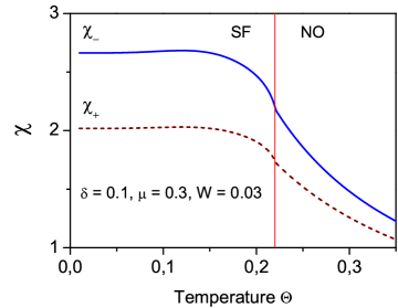
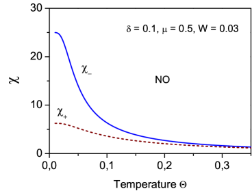
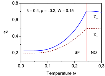
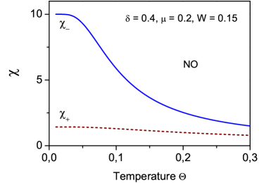
Figure 4: (Color online) Susceptibilities $\chi_{+}$ and $\chi_{-}$ as functions of temperature at various values of boson chemical potential.

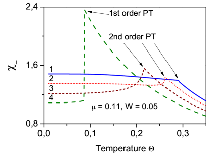
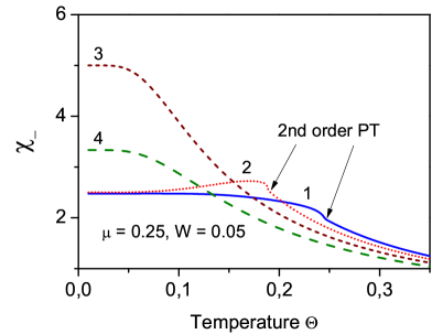
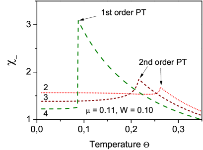
Figure 5: (Color online) Susceptibility $\chi_{-}$ as function of temperature in the region of NO-SF phase transition at different values of model parameters.

In figures 4 and 5 we show the graphs for susceptibility

$$\chi_{\pm}=\left.-\frac{2\pi}{\hbar^{2}}\langle\langle\hat{x}|\hat{x}\rangle\rangle_{\omega=0,\vec{q}}\right|_{d^{2}\Phi_{q}=\pm W}$$ (3.52)

as a function of temperature. The calculations were performed at various values of $\mu$, $\delta$ and $W$ meeting the condition $W<\delta/2$. As we can see, $\chi_{-}$ is greater than $\chi_{+}$; this gives an evidence for the dominance of potential instability with respect to modulation of particle displacements (with the wave vector at the boundary of Brillouin zone).

Susceptibility $\chi_{-}$ increases noticeably at a lowering of temperature in NO phase. However, at a further decrease of $T$ after transition to SF phase, a significant suppression of $\chi_{-}$ takes place. The $\chi_{-}$ function (just as $\chi_{+}$) approaches saturation (increasing or decreasing slightly, depending on value of $\delta$). In the majority of cases, there exists a peak of the $\chi_{-}$ function in the vicinity of the 1st order PT point. At this point, $\chi_{-}$ reaches a maximum value which remains finite in the considered range of the model parameter values. Consequently, the tendency to the displacement modulation, that is characteristic of NO phase, weakens when the NO-SF transition takes place and the BE condensate appears.

4 Conclusions

In this work, for the system of quantum particles in a lattice (Bose-atoms in optical lattice, adsorbed or intercalated particles in a crystal), we performed an investigation of the spectrum of collective vibrational excitations that appear at the displacements of a particle with respect to their equilibrium positions in local positions and which are connected with interactions between them. At a quantum description of displacements, we took into account the transitions of particles between the ground state and the first excited state only.

Such excitations, by their nature, are analogous to optical phonons in a usual crystal lattice. On the other hand, in the two-level approximation, they are similar to the Frenkel excitons or to excitations in the systems with double potential wells.

Calculation of the spectrum is performed in the framework of such a two-state model supposing that the quantum hopping of particles between the neighbouring positions in a lattice takes place in their excited state. Consideration is performed on the basis of the hard-core boson model.

We found the excitation spectrum in the random phase approximation using the Green’s function method. It is shown that the spectrum is of a band character and consists of positive and negative parts (among them, the second part is the mirror image of the first one). Only one positive branch [$\varepsilon_{1}(\vec{q})$] exists in the NO phase, while in the SF phase there appears an additional branch [$\varepsilon_{3}(\vec{q})$].

Positions, spectral weights of branches and widths of the corresponding bands change at the shift of the chemical potential of bosons and depend on temperature. A noticeable redistribution of the intensities of branches takes place in the SF phase at the change of $\mu$.

An additional branch [$\varepsilon_{3}(\vec{q})$] can become ‘‘soft’’ and go to zero at a certain value of $\mu$. However, such a behaviour does not lead to an instability in the system with respect to the modulation of particle displacements. The spectral weight of this mode also diminishes in this case and is equal to zero at this point. This fact is confirmed by calculation of the related susceptibility $\chi_{-}$ connected directly with Green’s function of displacements. The results show that in the case, when the boson system is stable in the NO phase, the transition to the SF phase and the subsequent lowering of $T$ (or decrease of $\mu$) do not give rise to instability. The possible displacement modulation could lead to the appearance of the so-called super-solid phase (with modulation of the BE condensate order parameter). In our case, however, the BE condensate remains uniform.

The analysis of the spectrum of phonon-like excitations in optical lattices and the investigation of its transformation and the appearance of new branches in the SF phase are possible with the use of Raman spectroscopy. Raman scattering intensity can be expressed in this case in terms of the Green’s function of particle displacements of the $\langle\langle\hat{x}|\hat{x}\rangle\rangle$ type, and the poles of this function will determine the Raman excitation spectrum (additional poles, appearing in the SF phase, manifest themselves as new Raman lines). Experimentally, such a technique was applied in [33] to study the spectrum of ultracold Bose-atoms excited to the upper Bloch band. Attention was paid to the observed features of scattering line profiles in a MI phase. Their explanation was given in terms of local transitions of bosons between ground and excited states in potential wells in a lattice. Theoretical analysis of Raman scattering intensity due to transitions to higher vibrational bands (in the case of sufficiently deep lattice and different number of particles per site) was performed in [34], as well as for the MI regime. The attention to differences between the intensity or amplitude of scattered light for SF and MI phases was directed in [35], where the possible experiments based on the Raman scattering-in-cavity technique were proposed. It is clear, on the whole, that Raman spectroscopy opens up new possibilities in the study of quantum states and the dynamics of Bose-atoms in the presence of BE condensate. However, more systematic investigations in this direction are needed. In this connection, a further development of the theory based on the calculation of the effective Raman coupling strength for specific cases and models is necessary.

Ukrainian 0

Збудження фононного типу у двостановiй моделi Бозе-Хаббарда I.В. Стасюк, О.В. Величко, О. Воробйов

             
Iнститут фiзики конденсованих систем НАН України, вул. I. Свєнцiцького, 1, 79011 Львiв, Україна