On the symplectic integration of the discrete nonlinear Schrödinger equation with disorder

Abstract

We present several methods, which utilize symplectic integration techniques based on two and three part operator splitting, for numerically solving the equations of motion of the disordered, discrete nonlinear Schrödinger (DDNLS) equation, and compare their efficiency. Our results suggest that the most suitable methods for the very long time integration of this one-dimensional Hamiltonian lattice model with many degrees of freedom (of the order of a few hundreds) are the ones based on three part splits of the system’s Hamiltonian. Two part split techniques can be preferred for relatively small lattices having up to $N\approx\;$70 sites. An advantage of the latter methods is the better conservation of the system’s second integral, i.e. the wave packet’s norm.

1 Introduction

Disordered systems are models of usually many degrees of freedom trying to mimic heterogeneity in nature. Typically they are obtained by attributing to one of the system’s parameters a different, random value for each degree of freedom. It is well-known that in linear disordered systems energy excitations remain localized. This phenomenon was first studied by Anderson in 1958 A58 and for this reason is usually called ‘Anderson localization’. This behavior plays an important role in several physical processes, like for example the conductivity of materials, the dynamics of Bose-Einstein condensates etc.

In the last decade the effect of nonlinearity on disordered systems has attracted extensive attention in theory and simulations VKF09_B11_MAP11_MAPS11_LBF12_MP12_MP13_LIF14 ; KKFA08 ; PS08 ; FKS09 ; GMS09 ; SKKF09 ; SF10 ; LBKSF10 ; BLSKF11 ; SGF13 ; ABSD14 , as well as in experiments SBFS07_LAPSMCS08_REFFFZMMI08 . A fundamental question in this context is what happens to energy localization in the presence of nonlinearities. Several studies of the disordered variants of two fundamental one-dimensional Hamiltonian lattice models, namely the Klein-Gordon (KG) oscillator chain and the discrete nonlinear Schrödinger equation (DDNLS), determined the statistical characteristics of energy spreading and showed that nonlinearity destroys localization FKS09 ; GMS09 ; SF10 ; LBKSF10 ; BLSKF11 . In these works the existence of different dynamical behaviors and spreading regimes was revealed, their particular dynamical characteristics were determined and their appearance was theoretically explained. The DDNLS model was used for the theoretical treatment of wave packet spreading, while numerics in both models were employed for verifying the obtained theoretical results.

The numerical integration of the KG model proved to be computationally easier than the DDNLS system, as the KG Hamiltonian can be readily split into two integrable parts (namely the kinetic and the potential energy). This splitting permits the application of several commonly used symplectic integrators (SIs) for the integration of the KG model, like for example the SABA₂ integrator with corrector LR01 , which proved to be a very efficient fourth order SI for this system FKS09 ; SKKF09 ; SF10 ; LBKSF10 ; BLSKF11 ; SGF13 . On the other hand, the numerical integration of the DDNLS model is a more complicated task, which requires the implementation of some specially designed techniques (see for example the appendices of SKKF09 ; BLSKF11 for more details). Nevertheless, the required CPU times did not allow the computation of the system’s evolution up to the same final times as for the KG model; typically for the same computational effort wave packets in the KG model were propagated in time up to one or two orders of magnitude longer than in the DDNLS system.

Although, nowadays it is common knowledge that energy spreading in disordered lattices is a chaotic process, the characteristics of this chaotic behavior have not been studied in detail. The first attempt to systematically investigate chaos in one-dimensional, disordered, nonlinear lattices was performed in SGF13 for the KG model. In that study the use of SIs was extended according to the so-called ‘tangent map method’ SG10_GS11_GES12 to integrate both the orbit itself, as well as a small deviation vector about it, whose evolution is needed for the computation of a chaos indicator like the maximum Lyapunov exponent (see for example S10 and references therein). These computations are easier for the KG model than for the DDNLS system and that is why the former system was chosen in SGF13 . In that paper it was shown that although chaotic dynamics slows down (as is indicated by the continuous decrease in time of the maximum Lyapunov exponent), it does not cross over into regular dynamics. Nevertheless, performing similar computations also for the DDNLS model is necessary for supporting the possible generality of the results obtained in SGF13 .

Thus, although our understanding of the dynamical evolution and the chaotic behavior of disordered lattices has been improved in recent years, several important questions remain open: Will wave packets continue spreading indefinitely, as current numerical simulations indicate KKFA08 ; PS08 ; FKS09 ; GMS09 ; SKKF09 ; SF10 ; LBKSF10 ; BLSKF11 ; SGF13 ; ABSD14 , or will they eventually exhibit a less chaotic behavior, leading to the halt of spreading, as is conjectured by some researchers JKA10_A11 ? How does wave packet’s chaoticity depend on the initial excitation, and how does it evolve in time? In order to address these questions we need to perform computationally expensive numerical simulations and investigate the asymptotic behavior of different disordered lattice models. Thus, the construction of numerical schemes, which will allow the accurate and efficient integration of multi-dimensional DDNLS models is imperative. Several such methods have been proposed and implemented in recent years, see e. g. SKKF09 ; BLSKF11 ; KS01 ; M13 ; GESBP13 ; SGBPE14 . In this work, we focus our attention to methods based on symplectic integration techniques and investigate their performance.

The paper is organized as follows. In Sect. 2, after a brief discussion of the properties of SIs, we describe integration methods that are based on the splitting of the DDNLS Hamiltonian in two integrable parts. Section 3 is devoted to symplectic integration techniques obtained by splitting the DDNLS Hamiltonian in three integrable parts. Then, in Sect. 4 we compare the performance of all these numerical schemes for the integration of the DDNLS system, while in Sect. 5 we summarize our results and present our conclusions.

2 Two part split integration schemes

Symplectic integrators are nowadays standard and widely implemented numerical techniques for Hamiltonian dynamics. Their use for the integration of the Hamilton equations of motion has two main advantages: it a) keeps the error of the computed value of the Hamiltonian function (which is an integral of motion, usually referred as the system’s ‘energy’) bounded, irrespectively of the total integration time, and b) results in efficient numerical procedures, as it allows the utilization of relatively large integration steps $\tau$, which lower the required CPU time. These characteristics make SIs the ideal tools for the long time integration of multidimensional DDNLS systems.

Symplectic integrators approximate the real solution of the Hamilton equations of motion by replacing the dynamics of the Hamiltonian system by appropriately chosen successive actions of other simpler (and usually integrable) functions, whose sum is the initial Hamiltonian. Usually, symplectic splitting methods are implemented by separating the Hamiltonian in two integrable parts (for an overview see for example (HLW02, , Sect. II.5)MQ02_MQ06_F06_BCM08 and references therein), although SIs based on three part splits have also been used GESBP13 ; SGBPE14 ; K96_C99_GBB08_QPRB10 .

In what follows we briefly describe the use of SIs for the integration of an autonomous Hamiltonian function which splits in two integrable parts. For this purpose, let us consider a system of $N$ degrees of freedom ($N$D) described by the Hamiltonian function $H(\vec{x})=h=\mbox{constant}$, where $\vec{x}=(\vec{q},\vec{p})$ represents the vector of generalized coordinates $\vec{q}=(q_{1},q_{2},\ldots,q_{N})$ and momenta $\vec{p}=(p_{1},p_{2},\ldots,p_{N})$. Then, the Hamilton equations of motion are $\frac{d\vec{x}}{dt}=\{\vec{x},H\}=L_{H}\vec{x}$, where $L_{H}=\{\cdot,H\}$ is a differential operator with $\{\cdot,\cdot\}$ being the Poisson bracket defined by $\{f,g\}=\sum_{l=1}^{N}\left(\frac{\partial f}{\partial q_{l}}\frac{\partial g}{\partial p_{l}}-\frac{\partial f}{\partial p_{l}}\frac{\partial g}{\partial q_{l}}\right)$, for any smooth functions $f(\vec{q},\vec{p})$ and $g(\vec{q},\vec{p})$. The formal solution of the equations of motion, for initial conditions $\vec{x}_{0}=\vec{x}(0)$, is $\vec{x}(\tau)=\sum_{k\geq 0}\frac{\tau^{k}}{k!}L_{H}^{k}\vec{x}_{0}=e^{\tau L_{H}}\vec{x}_{0}$.

Let us now assume that the Hamiltonian function can be split in two integrable parts as $H(\vec{x})=\mathcal{A}(\vec{x})+\mathcal{B}(\vec{x})$, so that the action of the operators $e^{\tau L_{\mathcal{A}}}$ and $e^{\tau L_{\mathcal{B}}}$ is known analytically. Then, a SI of order $n$ approximates the operator $e^{\tau L_{H}}$ by a product of $p$ operators $e^{a_{i}\tau L_{\mathcal{A}}}$ and $e^{b_{i}\tau L_{\mathcal{B}}}$ (which represent exact integrations over times $a_{i}\tau$ and $b_{i}\tau$ of Hamiltonians $\mathcal{A}(\vec{x})$ and $\mathcal{B}(\vec{x})$ respectively) according to $e^{\tau L_{H}}=e^{\tau\left(L_{\mathcal{A}}+L_{\mathcal{B}}\right)}=\prod_{i=1}^{p}e^{a_{i}\tau L_{\mathcal{A}}}e^{b_{i}\tau L_{\mathcal{B}}}+\mathcal{O}(\tau^{n+1})$. The constants $a_{i}$ and $b_{i}$ are chosen specifically to reach the desired order of the integrator.

The DDNLS system is a one-dimensional lattice model of $N$ coupled nonlinear oscillators described by the Hamiltonian BLSKF11 ; GESBP13 ; SGBPE14

$$H_{D}=\sum_{i=1}^{N}\frac{\epsilon_{i}}{2}\left(q_{i}^{2}+p_{i}^{2}\right)+\frac{\beta}{8}\left(q_{i}^{2}+p_{i}^{2}\right)^{2}-p_{i+1}p_{i}-q_{i+1}q_{i},$$ (1)

where $q_{i}$ and $p_{i}$ are, respectively, the generalized position and momentum of site $i$, the random on-site energy coefficients $\epsilon_{i}$ are chosen uniformly from the interval $\left[-W/2,W/2\right]$, with $W$ denoting the disorder strength, and $\beta\geq 0$ is the nonlinearity’s strength, while fixed boundary conditions ($q_{N+1}=p_{N+1}=0$) are imposed. This model has two integrals of motion as it conserves the energy $H_{D}$ (1) and the norm

$$S=\sum_{i=1}^{N}\frac{1}{2}\left(q_{i}^{2}+p_{i}^{2}\right).$$ (2)

The Hamiltonian (1) can be split in two integrable parts

$$\mathcal{A}=\sum_{i=1}^{N}\frac{\epsilon_{i}}{2}\left(q_{i}^{2}+p_{i}^{2}\right)+\frac{\beta}{8}\left(q_{i}^{2}+p_{i}^{2}\right)^{2}\,\,\mbox{ and }\,\,\mathcal{B}=\sum_{i=1}^{N}-p_{i+1}p_{i}-q_{i+1}q_{i},$$ (3)

whose operators $e^{\tau L_{\mathcal{A}}}$, $e^{\tau L_{\mathcal{B}}}$ can be obtained analytically com . In particular, the propagation of initial conditions $(q_{i},p_{i})$ at time $t$, to their final values $(q^{\prime}_{i},p^{\prime}_{i})$ at time $t+\tau$ is given by the operators

$$e^{\tau L_{\mathcal{A}}}:\left\{\begin{array}[]{lll}q^{\prime}_{i}&=&q_{i}\cos(\alpha_{i}\tau)+p_{i}\sin(\alpha_{i}\tau)\\ p^{\prime}_{i}&=&p_{i}\cos(\alpha_{i}\tau)-q_{i}\sin(\alpha_{i}\tau)\\ \end{array}\right.,\,\,i=1,2,\ldots,N,$$ (4)

$$e^{\tau L_{\mathcal{B}}}:(\vec{q}^{\prime},\vec{p}^{\prime})^{\mathrm{T}}=\mathbf{C}(\tau)\cdot(\vec{q},\vec{p})^{\mathrm{T}},$$ (5)

where $\alpha_{i}=\epsilon_{i}+\beta(q_{i}^{2}+p_{i}^{2})/2$, $\mathbf{C}(\tau)$ is a matrix whose expression is obtained in Appendix A, and (^T) denotes the transpose of a matrix. The operator $e^{\tau L_{\mathcal{A}}}$ has already been used in the literature BLSKF11 ; M13 ; GESBP13 ; SGBPE14 , while, to the best of our knowledge, this is the first time that the expression (5) of $e^{\tau L_{\mathcal{B}}}$ with respect to the matrix $\mathbf{C}(\tau)$ is reported. We note that since the integration step $\tau$ of SIs is typically kept constant, the matrix $\mathbf{C}(\tau)$ appearing in (5) remains constant for each numerical implementation of the operator $e^{\tau L_{\mathcal{B}}}$.

Based on this splitting we consider in our study several SIs of different orders. An extensively used simple SI of order two is the so-called leap-frog ($LF$) or Verlet integrator (see for example (HLW02, , Sect. I.3.1))

$$LF(\tau)=e^{\frac{\tau}{2}L_{\mathcal{A}}}e^{\tau L_{\mathcal{B}}}e^{\frac{\tau}{2}L_{\mathcal{A}}}.$$ (6)

This is an integrator of 3 steps, i.e. 3 individual applications of operators of integrable Hamiltonian functions. The $S\mathcal{A}\mathcal{B}\mathcal{A}_{2}$ integrator LR01

$$S\mathcal{A}\mathcal{B}\mathcal{A}_{2}(\tau)=e^{c_{1}\tau L_{\mathcal{A}}}e^{d_{1}\tau L_{\mathcal{B}}}e^{c_{2}\tau L_{\mathcal{A}}}e^{d_{1}\tau L_{\mathcal{B}}}e^{c_{1}\tau L_{\mathcal{A}}},$$ (7)

with $c_{1}=\frac{1}{2}\left(1-\frac{1}{\sqrt{3}}\right)$, $c_{2}=\frac{1}{\sqrt{3}}$, $d_{1}=\frac{1}{2}$, is another integrator of order two having 5 steps. The order of this integrator can be improved when the term $\{\mathcal{B},\{\mathcal{B},\mathcal{A}\}\}$ leads to an integrable system, as in the common situation of $\mathcal{A}$ being the usual kinetic energy and $\mathcal{B}$ the potential energy depending only on positions. In that case, the addition of two extra corrector steps at each end of the integration scheme increases its order from two to four. For the DDNLS Hamiltonian (1) we have

$$\{\mathcal{B},\mathcal{A}\}=\sum_{i=1}^{N}\alpha_{i}\left[q_{i}(p_{i-1}+p_{i+1})-p_{i}(q_{i-1}+q_{i+1})\right]$$ (8)

and consequently

$$\begin{array}[]{cl}\{\mathcal{B},\{\mathcal{B},\mathcal{A}\}\}=\displaystyle\sum_{i=1}^{N}\Bigg{\{}&\beta\Big{[}q_{i}(p_{i-1}+p_{i+1})-p_{i}(q_{i-1}+q_{i+1})\Big{]}^{2}+\\ &+\Big{(}\alpha_{i}-\alpha_{i-1}\Big{)}\par\Big{[}q_{i-1}^{2}+p_{i-1}^{2}+q_{i-1}q_{i+1}+p_{i-1}p_{i+1}\Big{]}+\\ &+\Big{(}\alpha_{i}-\alpha_{i+1}\Big{)}\Big{[}q_{i+1}^{2}+p_{i+1}^{2}+q_{i-1}q_{i+1}+p_{i-1}p_{i+1}\Big{]}\Bigg{\}},\end{array}$$ (9)

which does not seem to be integrable. Thus, we do not combine the $S\mathcal{A}\mathcal{B}\mathcal{A}_{2}$ integrator with a corrector term, as was done for example for the KG model SKKF09 .

We also consider two fourth order integrators: the one found by Forest and Ruth FR90 and by Yoshida Y90 having 7 steps

$$S^{4}(\tau)=e^{c_{1}\tau L_{\mathcal{A}}}e^{d_{1}\tau L_{\mathcal{B}}}e^{c_{2}\tau L_{\mathcal{A}}}e^{d_{2}\tau L_{\mathcal{B}}}e^{c_{2}\tau L_{\mathcal{A}}}e^{d_{1}\tau L_{\mathcal{B}}}e^{c_{1}\tau L_{\mathcal{A}}},$$ (10)

with $c_{1}=\frac{1}{2\left(2-2^{1/3}\right)}$, $c_{2}=\frac{1-2^{1/3}}{2\left(2-2^{1/3}\right)}$, $d_{1}=\frac{1}{2-2^{1/3}}$, $d_{2}=-\frac{2^{1/3}}{2-2^{1/3}}$, and the $\mathcal{A}\mathcal{B}\mathcal{A}864$ method introduced in BCFLMM13 having 15 steps. The particular values of the coefficients appearing in the expression of the $\mathcal{A}\mathcal{B}\mathcal{A}864$ SI are given in Table 3 of BCFLMM13 .

In Y90 symmetric compositions of second order integrators were used to construct higher order SIs. As a sixth order integrator we consider in our study the integrator produced by the composition method referred as ‘solution A’ in Y90 , because according to M95 it shows the best performance among the ones presented in Y90 . According to this technique, starting from any second order SI $S^{2}$, a sixth order integrator $S^{6}$ is constructed as

$$S^{6}(\tau)=S^{2}(w_{3}\tau)S^{2}(w_{2}\tau)S^{2}(w_{1}\tau)S^{2}(w_{0}\tau)S^{2}(w_{1}\tau)S^{2}(w_{2}\tau)S^{2}(w_{3}\tau).$$ (11)

The exact values of $w_{i}$, $i=0,1,2,3$ can be found in (HLW02, , Chap. V, Eq. (3.11)) and Y90 . Using the second order $S\mathcal{A}\mathcal{B}\mathcal{A}_{2}$ integrator (7) in (11) we construct the sixth order integrator $S^{6}_{S}$ having 29 steps.

3 Three part split integration schemes

In SGBPE14 several SIs based on a three part split of the DDNLS Hamiltonian were developed. For these methods the Hamiltonian (1) is written as the sum of the following three integrable parts

$$A=\sum_{i=1}^{N}\frac{\epsilon_{i}}{2}\left(q_{i}^{2}+p_{i}^{2}\right)+\frac{\beta}{8}\left(q_{i}^{2}+p_{i}^{2}\right)^{2},\,\,B=-\sum_{i=1}^{N}p_{i+1}p_{i}\,\,\mbox{ and }\,\,C=-\sum_{i=1}^{N}q_{i+1}q_{i}.$$ (12)

The operator $e^{\tau L_{A}}$ is exactly the same as operator $e^{\tau L_{\mathcal{A}}}$ (4), while the operators corresponding to parts $B$ and $C$ are given by

$$e^{\tau L_{B}}:\left\{\begin{array}[]{lll}p^{\prime}_{i}&=&p_{i}\\ q^{\prime}_{i}&=&q_{i}-(p_{i-1}+p_{i+1})\tau\\ \end{array}\right.,$$ (13)

$$e^{\tau L_{C}}:\left\{\begin{array}[]{lll}q^{\prime}_{i}&=&q_{i}\\ p^{\prime}_{i}&=&p_{i}+(q_{i-1}+q_{i+1})\tau\\ \end{array}\right..$$ (14)

We include in our study the following three part split SIs which showed a particularly good performance in SGBPE14 for the integration of the DDNLS model: $ABC^{4}_{[\text{Y}]}$, $SS^{4}$, $SS^{4}_{864}$ which are of order four, and the sixth order scheme $ABC^{6}_{[\text{SS}]}$. We note that schemes $ABC^{4}_{[\text{Y}]}$ and $ABC^{6}_{[\text{SS}]}$ are created by appropriate compositions of the basic three part split integrator of order two $ABC^{2}(\tau)=e^{\frac{\tau}{2}L_{A}}e^{\frac{\tau}{2}L_{B}}e^{\tau L_{C}}e^{\frac{\tau}{2}L_{B}}e^{\frac{\tau}{2}L_{A}}$ SGBPE14 ; K96_C99_GBB08_QPRB10 , and have 13 and 45 steps respectively. The other two methods, $SS^{4}$ and $SS^{4}_{864}$, are based on the performance of two successive two part splits of (1), i.e. we implement a two part split SI following the splitting (3) where the $\mathcal{B}$ part is split again in two parts (the $B$ and $C$ Hamiltonians of (12)) and is integrated by the $SABA_{2}$ integrator. The specifications of each scheme can be found in SGBPE14 .

4 Numerical results

In order to investigate the performance of the various SIs, we consider as a test case a particular, randomly chosen, disorder realization of (1) for $N=1000$ sites, set $W=4$ (i.e. $\epsilon_{i}\in[-2,2]$) and $\beta=0.72$, and follow in time the evolution of an initially homogeneous excitation of the central 21 sites of the lattice. The initial norm density of the excited sites is set to unity and consequently the wave packet’s norm (2) is $S=S(0)=21$. Initially each excited site gets a random phase. The particular random configuration we consider in our simulations results to a total energy $H_{D}\approx-28.501$. We note that this configuration corresponds to the so-called ‘strong chaos’ spreading regime studied in LBKSF10 .

To evaluate the performance of each tested SI we check whether the obtained solutions correctly capture the wave packet dynamics by monitoring the time evolution of the second moment $m_{2}$ of the wave packet’s norm distribution $z_{i}=(q_{i}^{2}+p_{i}^{2})/(2S)$ FKS09 ; SKKF09 ; LBKSF10 ; BLSKF11 ; GESBP13 ; SGBPE14 . In addition, we monitor the preservation of the values of the two integrals $H_{D}$ (1) and $S$ (2) by keeping track of the absolute relative errors of the energy $E_{r}(t)=|[H_{D}(t)-H_{D}(0)]/H_{D}(0)|$, and the norm $S_{r}(t)=|[S(t)-S(0)]/S(0)|$. We also register the required CPU time $T_{c}$ needed for performing each simulation.

In Fig. 1 we present results obtained by the two part split integrators discussed in Sect. 2: $LF$ (6) [blue curves], $S\mathcal{A}\mathcal{B}\mathcal{A}_{2}$ (7) [green curves], $S^{4}$ (10) [brown curves], $\mathcal{A}\mathcal{B}\mathcal{A}864$ [yellow curves] and $S^{6}$ (11) [red curves]. The integration time step $\tau$ of each method was chosen so that all schemes keep the relative energy error bounded by practically the same value $E_{r}\approx 10^{-6}$ [Fig. 1(a)]. Additionally, all these two part split SIs preserve well the numerical value of the norm $S$ (2), since the corresponding $S_{r}$ quantities attain relatively small values [Fig. 1(b)] (although these values clearly increase in time). This happens because the norm $S$ (2) is an integral of motion of both the $\mathcal{A}$ and $\mathcal{B}$ Hamiltonians of (3), as the direct computation of its time derivative in both systems shows ($\frac{dS}{dt}=\{S,\mathcal{A}\}=0$ and $\frac{dS}{dt}=\{S,\mathcal{B}\}=0$). In addition, all integrators succeed to correctly describe the system’s dynamics as they give practically the same time evolution of $m_{2}$ [Fig. 1(c)]. From the results, of Fig. 1(d) we see that the fourth order $\mathcal{A}\mathcal{B}\mathcal{A}864$ together with the sixth order scheme $S^{6}$ (11) show the best numerical performance as they both require the least CPU time among all tested methods.

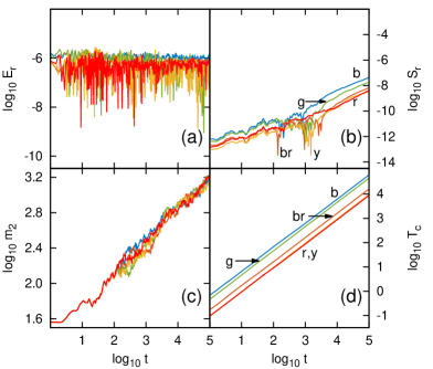
Figure 1: (Color online) Results for the integration of $H_{D}$ (1) by the two part split SIs $LF$ for $\tau=0.0025$, $S\mathcal{A}\mathcal{B}\mathcal{A}_{2}$ for $\tau=0.01$, $S^{4}$ for $\tau=0.05$, $\mathcal{A}\mathcal{B}\mathcal{A}864$ for $\tau=0.175$ and $S^{6}$ for $\tau=0.25$ [(b) blue; (g) green; (br) brown; (y) yellow; (r) red]: time evolution of the logarithm of (a) the absolute relative energy error $E_{r}(t)$, (b) the absolute relative norm error $S_{r}(t)$ (c) the second moment $m_{2}(t)$, and (d) the required CPU time $T_{c}(t)$ in seconds. Note that in panel (d) the red and yellow curves practically overlap.

In Fig. 2 we see results obtained by the three part split integrators considered in our study (see Sect. 3): the fourth order schemes $ABC^{4}_{[\text{Y}]}$ [blue curves], $SS^{4}$ [red curves], $SS^{4}_{864}$ [yellow curves] and the sixth order integrator $ABC^{6}_{[\text{SS}]}$ [green curves]. Again, all integrators keep the relative energy error small ($E_{r}\lesssim 10^{-6}$) for the particular choices of the integration steps $\tau$ [Fig. 2(a)] and reproduce correctly the evolution of the wave packet’s second moment [Fig. 2(c)]. A difference with respect to the two part split SIs of Fig. 1 is that the values of the relative norm error $S_{r}$ [Fig. 2(b)] are much larger than the ones reported in Fig. 1(b). The reason for this is the fact that the norm $S$ (2) is an integral of motion of $\mathcal{B}$ (3) but not of $B$ and $C$ (12) separately. Furthermore, we note that also for three part split methods $S_{r}$ increases in time although its increase rate is smaller than the one seen in Fig. 1(b). From Fig. 2(d) we see that the sixth order integrator $ABC^{6}_{[\text{SS}]}$ needs the least CPU time among the tested SIs. The $SS^{4}_{864}$ integrator exhibits the second best behavior, as it requires a slightly larger CPU time than $ABC^{6}_{[\text{SS}]}$, but keeps $S_{r}$ to acceptable levels (smaller than $ABC^{4}_{[\text{Y}]}$ [Fig. 2(b)], with which they require practically the same CPU time [Fig. 2(d)]).

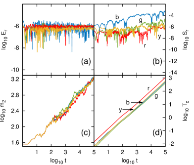
Figure 2: (Color online) Results for the integration of $H_{D}$ (1) by the three part split SIs $ABC^{4}_{[\text{Y}]}$ for $\tau=0.05$, $SS^{4}$ for $\tau=0.05$, $SS^{4}_{864}$ for $\tau=0.125$ and $ABC^{6}_{[\text{SS}]}$ for $\tau=0.225$ [(b) blue; (r) red; (y) yellow; (g) green]. The panels are as in Fig. 1.

It is worth noting that all three part split integrators of Fig. 2 require considerably less CPU time than the two part split schemes of Fig. 1, as a direct comparison of Fig. 1(d) and Fig. 2(d) reveals, despite the fact that more operators are involved in the three part split methods. This happens because the application of $e^{\tau L_{\mathcal{B}}}$ (5) is computationally very expensive, especially for high values of $N$. To illustrate the dependence of the performance of the integration schemes on the number of the system’s degrees of freedom $N$, we consider the best performing schemes among the two part split methods (here we used $\mathcal{A}\mathcal{B}\mathcal{A}864$ as preliminary tests showed a slightly better performance than for $S^{6}$) and the three part split techniques (i.e. $ABC^{6}_{[\text{SS}]}$) and monitor their behavior when $N$ is varied.

In Fig. 3(a) we report the CPU time $T_{c}$ needed for each SI to integrate a lattice of $N$ sites up to $t=10^{4}$ for various values of $N$ up to $N=500$. For each simulation the integration time step was kept constant to $\tau=0.175$ for the $\mathcal{A}\mathcal{B}\mathcal{A}864$ SI and to $\tau=0.225$ for the $ABC^{6}_{[\text{SS}]}$ one. The time average (over the whole duration of each simulation) of the relative energy error $\langle E_{r}\rangle$ for each method is seen in Fig. 3(b). We see that for the particular choice of integration steps $\langle E_{r}\rangle$ does not change significantly as $N$ varies, remaining close to values around $10^{-6}$ for both methods.

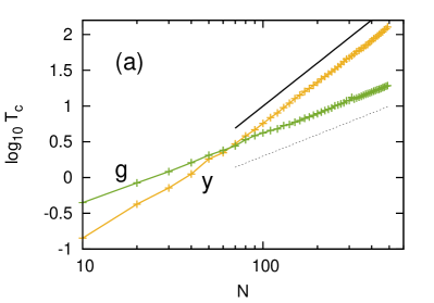
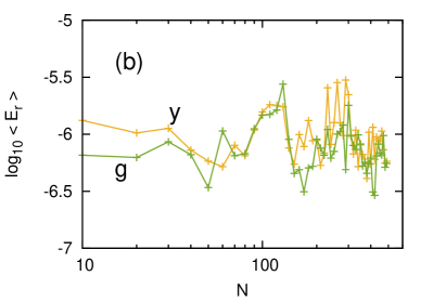
Figure 3: (Color online) The logarithm of (a) the required CPU time $T_{c}$ and (b) the time averaged relative energy error $\langle E_{r}\rangle$ for the integration of the DDNLS model (1) up to the final integration time $t=10^{4}$ by the $\mathcal{A}\mathcal{B}\mathcal{A}864$ [(y) yellow curves] and the $ABC^{6}_{[\text{SS}]}$ [(g) green curves] methods for various values of the number of sites $N$. In (a) the slopes 2 and 1 are denoted by black solid and dotted lines respectively.

From the results of Fig. 3(a) we see that the two part split SI $\mathcal{A}\mathcal{B}\mathcal{A}864$ requires less CPU time than the three part split scheme $ABC^{6}_{[\text{SS}]}$ for values of $N\lesssim 70$. The difference between the two methods becomes more pronounced as $N$ increases. The obtained results indicate that $T_{c}\propto N^{2}$ for $\mathcal{A}\mathcal{B}\mathcal{A}864$, while $T_{c}\propto N$ for $ABC^{6}_{[\text{SS}]}$, as indicated by the black lines shown in Fig. 3(a). This behavior can be easily understood from the different computational complexity of the operators used in these two splitting schemes. While operators $e^{\tau L_{B}}$(13) and $e^{\tau L_{C}}$ (14) basically require the addition of two vectors, the multiplication of matrix $\mathbf{C}(\tau)$ with vector $\mathbf{x}$ in (5) requires $N^{2}$ operations for each application of $\mathrm{e}^{\tau L_{\mathcal{B}}}$. Therefore, the results of Fig. 3(a) clearly show that the three part split schemes should be used for large lattices, while relatively small lattices ($N$ of the order of a few tens) are better to be integrated by a two part split SI. Let us note, that the behavior shown in Fig. 3(a) is independent of the system’s spreading regimes as we obtained qualitatively similar results (not reported here) for initial conditions in the so-called ‘weak chaos’ and ‘selftrapping’ regimes (see LBKSF10 for more details on the definition of these regimes).

5 Summary and conclusions

The numerical integration of the discrete nonlinear Schrödinger equation with disorder is computationally very challenging. In this work we presented and compared various symplectic splitting techniques suitable to perform this task with the required accuracy.

For SIs based on the splitting of the Hamiltonian in two integrable parts, we explicitly presented (to the best of our knowledge for the first time) an analytical solution for the operator $\mathrm{e}^{\tau L_{\mathcal{B}}}$ (5). Besides being more compact, this form has the advantage that various two part split numerical methods are readily available from the literature. Using several suitable schemes we integrated the corresponding equations of motion and showed that for this splitting the norm of the wave packet $S$ (2) is preserved naturally to a very high accuracy.

To investigate the importance of these results we also integrated the DDNLS system with several three part split SIs, which are already known to be very well suited for this problem SGBPE14 . We found that it is possible to obtain results with the same level of relative energy error much faster with these three part split methods. Furthermore, we showed that (and also explained why) the relative norm error $S_{r}$ is much larger with respect to the two part schemes.

We also investigated how the performance of these integration schemes depend on the number of degrees of freedom. For small lattices (with $N\lesssim 70$) the two part split $\mathcal{A}\mathcal{B}\mathcal{A}864$ scheme proved to be the most efficient one among all tested methods since it required the least CPU time, while at the same time gave very accurate results. Except for very high accuracy needs three part SIs should be used for larger lattices since their computational complexity grows linearly with $N$, and not like $N^{2}$ as is the case for two part split methods. We note that from the tested three part split integrators the $ABC^{6}_{[SS]}$ method showed the best performance.

Appendix A Determination of matrix $\mathbf{C}(\tau)$ of equation (5)

The equations of motion for the Hamiltonian $\mathcal{B}$ of (3) can be written in the form

$$\dot{\vec{x}}^{\mathrm{T}}=\mathbf{B}\vec{x}^{\mathrm{T}}=\left(\begin{array}[]{cc}\mathbf{0}&\mathbf{A}\\ \mathbf{-A}&\mathbf{0}\\ \end{array}\right)\vec{x}^{\mathrm{T}},$$ (15)

where $\mathbf{A}$, $\mathbf{B}$ are respectively $N\times N$ and $2N\times 2N$ constant matrices, while $\mathbf{0}$ is the $N\times N$ matrix having all its elements equal to zero. The $\mathbf{A}$ matrix is a tridiagonal matrix with all the elements of its main diagonal equal to zero ($\mathbf{A}_{i,i}=0$, $i=1,2,\ldots,N$), while all the elements of the first diagonals above and below the main one are equal to $-1$ ($\mathbf{A}_{i,i+1}=\mathbf{A}_{i-1,i}=-1$). The solution of system (15) for a time step $\tau$ is

$$\vec{x}^{\mathrm{T}}(t+\tau)=e^{\mathbf{B}\tau}\vec{x}^{\mathrm{T}}(t)=\sum_{k=0}^{\infty}\frac{1}{k!}(\mathbf{B}\tau)^{k}\vec{x}^{\mathrm{T}}(t)=\mathbf{C}(\tau)\vec{x}^{\mathrm{T}}(t).$$ (16)

It can be easily seen by induction that

$$\mathbf{B}^{2k}=(-1)^{k}\left(\begin{array}[]{cc}\mathbf{A}^{2k}&\mathbf{0}\\ \mathbf{0}&\mathbf{A}^{2k}\\ \end{array}\right),\,\,\,\,\mathbf{B}^{2k+1}=(-1)^{k}\left(\begin{array}[]{cc}\mathbf{0}&\mathbf{A}^{2k+1}\\ \mathbf{-A}^{2k+1}&\mathbf{0}\\ \end{array}\right),\,\,\,k\in\mathbb{N},$$ (17)

and consequently, matrix $\mathbf{C}(\tau)$ in (16) can be written as

$$\mathbf{C}(\tau)=e^{\mathbf{B}\tau}=\left(\begin{array}[]{rr}\cos(\mathbf{A}\tau)&\sin(\mathbf{A}\tau)\\ -\sin(\mathbf{A}\tau)&\cos(\mathbf{A}\tau)\\ \end{array}\right)$$ (18)

with

$$\cos(\mathbf{A}\tau)=\sum_{k=0}^{\infty}\frac{(-1)^{k}}{(2k)!}\mathbf{A}^{2k}\tau^{2k},\,\,\,\,\sin(\mathbf{A}\tau)=\sum_{k=0}^{\infty}\frac{(-1)^{k}}{(2k+1)!}\mathbf{A}^{2k+1}\tau^{2k+1}.$$ (19)

The evaluation of the elements of matrices $\cos(\mathbf{A}\tau)$ and $\sin(\mathbf{A}\tau)$ can be obtained through the determination of the eigenvalues and eigenvectors of matrix $\mathbf{A}$ itself (see for example S86 ). In particular, the eigenvalues $\lambda_{k}$ of $\mathbf{A}$ are simple and symmetric with respect to zero, and are given by

$$\lambda_{k}=-2\cos\left(\frac{k\pi}{N+1}\right),\,\,\,\,k=1,2,\ldots,N,$$ (20)

while its eigenvectors are orthogonal (since $\mathbf{A}$ is symmetric) and have the form

$$\vec{v}_{k}=\frac{1}{V_{k}}\Bigg{(}\sin\left(\frac{k\pi}{N+1}\right),\sin\left(\frac{2k\pi}{N+1}\right),\dots,\sin\left(\frac{Nk\pi}{N+1}\right)\Bigg{)},$$ (21)

with

$$V_{k}^{2}=\|\vec{v}_{k}\|^{2}=\sum_{j=1}^{N}\sin^{2}\left(\frac{jk\pi}{N+1}\right)=\frac{2N+1}{4}-\frac{\sin\left(\frac{2N+1}{N+1}k\pi\right)}{4\sin(\frac{k\pi}{N+1})},$$ (22)

where $\|\cdot\|$ denotes the usual Euclidean norm of a vector. The identity

$$\sum_{j=0}^{N}\cos\left(jx\right)=\frac{1}{2}\left[1+\frac{\sin\left[\left(N+\frac{1}{2}\right)x\right]}{\sin\left(\frac{x}{2}\right)}\right]$$ (23)

(see for example (GR07, , Eq. 1.342-2.)) was used to obtain the last equality of (22). The matrix $\mathbf{S}$ having as columns the eigenvectors (21), i.e. $\mathbf{S}=(\vec{v}_{1}^{\mathrm{T}},\,\,\vec{v}_{2}^{\mathrm{T}},\,\,\ldots,\,\,\vec{v}_{N}^{\mathrm{T}})$, can be used to diagonalize $\mathbf{A}$. Thus, $\mathbf{A}=\mathbf{S}\mathbf{D}\mathbf{S}$ (since $\mathbf{S}^{-1}=\mathbf{S}^{\mathrm{T}}=\mathbf{S}$), with $\mathbf{D}$ being the diagonal $N\times N$ matrix having as diagonal elements the eigenvalues (20), i.e. $\mathbf{D}=\mbox{diag}(\lambda_{1},\lambda_{2},\ldots,\lambda_{N})$. Then, from (19) we see that matrices $\cos(\mathbf{A}\tau)$ and $\sin(\mathbf{A}\tau)$ defining $\mathbf{C}(\tau)$ in (18) can be written as $\cos(\mathbf{A}\tau)=\mathbf{S}\mathbf{D}_{c}\mathbf{S}$ and $\sin(\mathbf{A}\tau)=\mathbf{S}\mathbf{D}_{s}\mathbf{S}$ with $\mathbf{D}_{c}=\mbox{diag}(\cos(\lambda_{1}\tau),\cos(\lambda_{2}\tau),\ldots,\cos(\lambda_{N}\tau))$, $\mathbf{D}_{s}=\mbox{diag}(\sin(\lambda_{1}\tau),\sin(\lambda_{2}\tau),\ldots,\sin(\lambda_{N}\tau))$. Consequently, $\mathbf{C}(\tau)$ (18) is a constant matrix for a fixed integration time step $\tau$.

References

- (1) P. W. Anderson, Phys. Rev. 109, 1492 (1958)
- (2) H. Veksler, Y. Krivolapov, S. Fishman, Phys. Rev. E 80, 037201 (2009); D. M. Basko, Annals Phys. 326, 1577 (2011); M. Mulansky, K. Ahnert, A. Pikovsky, Phys. Rev. E 83, 026205 (2011); M. Mulansky, K. Ahnert, A. Pikovsky, D. L. Shepelyansky, J. Stat. Phys. 145, 1256 (2011); T. V. Laptyeva, J. D. Bodyfelt, S. Flach, Europhys. Lett. 98, 60002 (2012); M. Mulansky, A. Pikovsky, Phys. Rev. E 86, 056214 (2012); M. Mulansky, A. Pikovsky, New J. Phys. 15, 053015 (2013); T. V. Laptyeva, M. V. Ivanchenko, S. Flach, J. Phys. A 47, 493001 (2014)
- (3) G. Kopidakis, S. Komineas, S. Flach, S. Aubry, Phys. Rev. Lett. 100, 084103 (2008)
- (4) A. S. Pikovsky, D. L. Shepelyansky, Phys. Rev. Lett. 100, 094101 (2008)
- (5) S. Flach, D. O. Krimer, Ch. Skokos, Phys. Rev. Lett. 102, 024101 (2009); ibid. 209903 (2009)
- (6) I. García-Mata, D. L. Shepelyansky, Phys. Rev. E 79, 026205 (2009)
- (7) Ch. Skokos, D. O. Krimer, S. Komineas, S. Flach, Phys. Rev. E 79, 056211 (2009); ibid. 89, 029907 (2014)
- (8) Ch. Skokos, S. Flach, Phys. Rev. E 82, 016208 (2010)
- (9) T. V. Laptyeva, J. D. Bodyfelt, D. O. Krimer, Ch. Skokos, S. Flach, Europhys. Lett. 91, 30001 (2010)
- (10) J. D. Bodyfelt, T. V. Laptyeva, Ch. Skokos, D. O. Krimer, S. Flach, Phys. Rev. E 84, 016205 (2011)
- (11) Ch. Skokos, I. Gkolias, S. Flach, Phys. Rev. Let. 111, 064101 (2013)
- (12) Ch. Antonopoulos, T. Bountis, Ch. Skokos, L. Drossos, Chaos 24 024405 (2014)
- (13) T. Schwartz, G. Bartal, S. Fishman, M. Segev, Nature 446, 52 (2007); Y. Lahini, A. Avidan, F. Pozzi, M. Sorel, R. Morandotti, D. N. Christodoulides, Y. Silberberg, Phys. Rev. Lett. 100, 013906 (2008); G. Roati, C. D’Errico, L. Fallani, M. Fattori, C. Fort, M. Zaccanti, G. Modugno, M. Modugno, M. Inguscio, Nature 453, 895 (2008)
- (14) J. Laskar, P. Robutel, Cel. Mech. Dyn. Astr. 80 39 (2001)
- (15) Ch. Skokos, E. Gerlach, Phys. Rev. E 82, 036704 (2010); E. Gerlach, Ch. Skokos, Discr. Cont. Dyn. Syst. – Supp. 2011, 475 (2011); E. Gerlach, S. Eggl, Ch. Skokos, Int. J. Bifurc. Chaos 22, 1250216 (2012)
- (16) Ch. Skokos, Lect. Notes Phys. 790, 63 (2010)
- (17) M. Johansson, G. Kopidakis, S. Aubry, Europhys. Lett. 91, 50001 (2010); S. Aubry, Int. J. Bifurc. Chaos 21, 2125 (2011)
- (18) D. A. Karpeev, C. M. Schober, Math. Comput. Simul. 56, 145 (2001)
- (19) M. Mulansky, ArXiv:physics.comp-ph/1304.1608 (2013)
- (20) E. Gerlach, S. Eggl, Ch. Skokos, J. D. Bodyfelt, G. Papamikos, in Proceedings of the 10th HSTAM International Congress on Mechanics, ArXiv:nlin.CD/1306.0627 (2013)
- (21) Ch. Skokos, E. Gerlach, J. D. Bodyfelt, G. Papamikos, S. Eggl, Phys. Let. A 378, 1809 (2014)
- (22) E. Hairer, C. Lubich, G. Wanner, Geometric Numerical Integration. Structure-Preserving Algorithms for Ordinary Differential Equations (Springer Series in Computational Mathematics Vol. 31, Springer, New York, 2002)
- (23) R. I. McLachan, G. R. W. Quispel, Acta Num. 11, 341 (2002); R. I. McLachan, G. R. W. Quispel, J. Phys. A 39, 5251 (2006); E. Forest, J. Phys. A 39, 5321 (2006); S. Blanes, F. Casas, A. Murua, Bol. Soc. Esp. Mat. Apl. 45, 89 (2008)
- (24) P.-V. Koseleff, Fields Inst. Comm. 10, 103 (1996); J. E. Chambers, Mon. Not. R. Astron. Soc. 304, 793 (1999); K. Goździewski, S. Breiter, W. Borczyk, Mon. Not. R. Astron. Soc. 383, 989 (2008); T. Quinn, R. P. Perrine, D. C. Richardson, R. Barnes, Astron. J. 139, 803 (2010)
- (25) We note that in BLSKF11 it was incorrectly stated that ‘Hamiltonian is not integrable, and thus the operator cannot be written explicitly’.
- (26) E. Forest, R. D. Ruth, Physica D 43, 105 (1990)
- (27) H. Yoshida, Phys. Lett. A 150, 262 (1990)
- (28) S. Blanes, F. Casas, A. Farrés, J. Laskar, J. Makazaga, A. Murua, App. Num. Math. 68, 58 (2013)
- (29) R. I. McLachan, SIAM J. Sci. Comput. 16, 151 (1995)
- (30) G. D. Smith, Numerical Solution of Partial Differential Equations: Finite Difference Methods, Third edition. (Oxford Applied Mathematics & Computing Science Series, Oxford University Press, New York, 1986) p. 156
- (31) I. S. Gradshteyn, I. M. Ryzhik, Table of Integrals, Series and Products, Seventh edition (Elsevier, Burlington, 2007) p. 37