Inflation model constraints from data released in 2015

Abstract

We provide the latest constraints on the power spectra of both scalar and tensor perturbations from the CMB data (including Planck 2015, BICEP2 & Keck Array experiments) and the new BAO scales from SDSS-III BOSS observation. We find that the inflation model with a convex potential is not favored and both the inflation model with a monomial potential and the natural inflation model are marginally disfavored at around $95\%$ confidence level. But both the Brane inflation model and the Starobinsky inflation model fit the data quite well.

I Introduction

In the past three decades, the inflation model Starobinsky:1980te ; Guth:1980zm ; Linde:1981mu ; Albrecht:1982wi was taken as the standard paradigm of the very early Universe. It not only resolves the flatness, horizon and monopole problems in the hot big bang model, but also generates the primordial density perturbations seeding the anisotropies in the cosmic microwave background (CMB) and the large-scale structure in our Universe. The simple inflation model predicts that the power spectra of both primordial scalar and tensor perturbations are adiabatic, Gaussian and nearly scale-invariant. In particular, the amplitude of primordial tensor perturbations is determined by the energy scale of inflation. Actually the primordial perturbations contribute to the anisotropies and polarizations of CMB as well as CMB lensing, which can be precisely measured by the ground-based or satellite CMB experiments, for example the Planck satellite Adam:2015rua ; Ade:2015lrj . Therefore one can estimate the cosmological parameters and explore the nature of inflation by using the CMB data.

The excess of B-mode power over the base lensed-$\Lambda$CDM expectation detected by BICEP2 Ade:2014xna can be explained by the polarized thermal dust, not the primordial gravitational waves Mortonson:2014bja ; Flauger:2014qra . Subtracting the contributions to the CMB B-mode from Galactic polarized dust measured by Planck collaboration in Adam:2014bub , the tensor-to-scalar ratio $r\lesssim 0.1$ at $95\%$ confidence level (C.L.) was obtained in Cheng:2014pxa which was confirmed by a joint analysis of B-mode polarization data of BICEP2/Keck Array and Planck (BKP) in Ade:2015tva . Furthermore, because of the tight constraint on the tensor-to-scalar ratio, the chaotic inflation model with a potential $V(\phi)\propto\phi^{2}$ was disfavored at more than $2\sigma$ C.L. in Cheng:2014pxa . All of these results are confirmed by the Planck 2015 results Ade:2015lrj in which the scalar spectral index $n_{s}=0.968\pm 0.006$ at $68\%$ C.L. and the tensor-to-scalar ratio $r_{0.002}<0.11$ at $95\%$ C.L. by fitting the Planck TT,TE,EE+lowP+lensing combination (P15).

Recently BICEP2 & Keck Array CMB polarization experiments released the B-mode polarization data up to and including the 2014 observing season in Array:2015xqh . This dataset includes the first Keck Array B-mode data at $95$ GHz. The BICEP2 & Keck Array B-mode data (BK14) implies $r_{0.05}<0.09$ ($95\%$ C.L.). Combining with Planck 2015 TT+lowP+lensing and some other external data, the upper bound on $r$ becomes $r_{0.05}<0.07$ ($95\%$ C.L.) Array:2015xqh in the base $\Lambda$CDM+$r$ model. This constraint on $r$ is the strongest one to date, even though it is model-dependent in some sense.

In addition, the Baryon Acoustic Oscillation (BAO) data can significantly break the degeneracies between cosmological parameters. Recently, the BAO distance scale measurements were updated via an anisotropic analysis of BAO scale in the correlation function Cuesta:2015mqa and power spectrum Gil-Marin:2015nqa of the CMASS and LOWZ galaxy samples from Data Release 12 of the SDSS-III Baryon Oscillation Spectroscopic Survey (BOSS DR12). The total volume probed in DR12 has a $10\%$ increment from DR11 and the experimental uncertainty has been reduced. In this paper, the BAO data we will adopt include 6dFGS Beutler:2011hx , MGS Ross:2014qpa , BOSS DR12 CMASS Gil-Marin:2015nqa and LOWZ Gil-Marin:2015nqa (BAO15).

In this paper we will make a joint analysis of the recently released CMB and BAO data to constrain the cosmological parameters and the inflation models. Our paper is arranged as follows. In Sec. II, we constrain the power spectra of both scalar and tensor perturbations by using the data combination of P15+BK14+BAO15. In Sec. III, we will test several inflation models in two different methods. The summary and discussion are included in Sec. IV.

II Constraints on the power spectra of scalar and tensor perturbations

In this section, we will make a joint analysis of P15+BK14+BAO15 dataset to constrain the cosmological parameters in the base $\Lambda$CDM+$r$ model and the other two extended models.

In general, the power spectra of primordial scalar and tensor perturbations can be parameterized as follows

$$P_{s}(k) = A_{s}\left(\frac{k}{k_{p}}\right)^{n_{s}-1+\frac{1}{2}\frac{dn_{s}}{d\ln k}\left(\ln\frac{k}{k_{p}}\right)+\frac{1}{6}\frac{d^{2}n_{s}}{d\ln k^{2}}\left(\ln\frac{k}{k_{p}}\right)^{2}}\ ,$$ (1)

$$P_{t}(k) = A_{t}\left(\frac{k}{k_{p}}\right)^{n_{t}}\ ,$$ (2)

where $A_{s}$ and $A_{t}$ denote the amplitudes of scalar and tensor power spectra at the pivot scale $k_{p}$, $n_{s}$ and $n_{t}$ denote the spectral indices of scalar and tensor power spectra, $n_{\textrm{run}}\equiv dn_{s}/d\ln k$ and $n_{\textrm{run,run}}\equiv d^{2}n_{s}/d\ln k^{2}$ denote the running and the running of running of scalar spectral index. In this paper, we set the pivot scale as $k_{p}=0.01~{}\textrm{Mpc}^{-1}$. The spectral index of tensor power spectrum is set as $n_{t}=-A_{t}/(8A_{s})$ which is the consistency relation for the canonical single-field slow-roll inflation model Liddle:1992wi . In principle, $n_{t}$ can be taken as a free parameter. However, $n_{t}$ cannot be well constrained by the current observations Cheng:2014ota ; Huang:2015gka ; Cabass:2015jwe , even though $n_{t}\simeq 0$ is consistent with the current datasets. The measurement on $n_{t}$ is expected to be improved by some forthcoming experiments Huang:2015gca .

In this paper we consider three cosmological models. The first one is the base $\Lambda$CDM+$r$ model in which there are seven free parameters: the baryon density today $(\Omega_{b}h^{2})$, the cold dark matter density today $(\Omega_{c}h^{2})$, the $100\times$ angular scale of the sound horizon at last-scattering ($100\theta_{\rm MC}$), the Thomson scattering optical depth due to the reionization $(\tau)$, the amplitude of scalar power spectrum $(A_{s})$, the spectral index of scalar power spectrum $(n_{s})$ and the tensor-to-scalar ratio $(r)$. The second one is the base $\Lambda$CDM+$r$+nrun model where the running of scalar spectral index ($dn_{s}/d\ln k$) is included as an additional free parameter. The third one is the base $\Lambda$CDM+$r$+nrun+nrunrun model in which an additional parameter, namely the running of running ($d^{2}n_{s}/d\ln k^{2}$), is added.

The BAO data and $1\sigma$ uncertainty of BOSS DR12 LOWZ and CMASS samples are listed in Tab. 1.

$z_{eff}$	BOSS DR12	$H(z_{eff})r_{d}[10^{3}\textrm{km}\cdot s^{-1}]$	$D_{A}(z_{eff})/r_{d}$	$\rho_{D_{A},H}$
$0.32$	LOWZ	$11.64\pm 0.70$	$6.76\pm 0.15$	$0.35$
$0.57$	CMASS	$14.66\pm 0.42$	$9.47\pm 0.13$	$0.54$

Table 1: The distance measurement from the anisotropic analysis of BAO scale in the CMASS and LOWZ galaxy samples released by SDSS-III BOSS DR12 Gil-Marin:2015nqa .

Their consensus values are listed here, which are used in this paper. Here $z_{eff}$ denotes the effective redshift for CMASS and LOWZ samples, respectively. $H(z_{eff})$ and $D_{A}(z_{eff})$ are Hubble parameter and angular diameter distance at redshift $z_{eff}$, respectively. $r_{d}$ denotes the comoving sound horizon at the redshift of baryon drag epoch. In addition, $\rho_{D_{A},H}$ is the normalized correlation between $D_{A}(z_{eff})$ and $H(z_{eff})$.

We can add a likelihood of the above BAO scales into our data analysis. The likelihood is given by

$$-2\ln\mathcal{L}=\sum_{k=1}^{2}\left(D^{data}-D^{model}\right)^{T}_{k}C_{k}^{-1}\left(D^{data}-D^{model}\right)_{k}\ ,$$ (3)

where $k=1$ for LOWZ and $k=2$ for CMASS. We denote $D^{data}_{k}\equiv\left(Hr_{d},D_{A}r_{d}\right)^{T}_{k}$ for the observational BAO data in Tab. 1. Calculated by CAMB Lewis:1999bs ; camb2012 , $D^{model}_{k}$ denote the corresponding theoretical predictions of cosmological models. We denote $C_{k}$ as the covariance matrix, namely

$$C_{k}=\left(\begin{array}[]{cc}\sigma_{D_{A}}^{2}&\rho_{D_{A},H}\sigma_{D_{A}}\sigma_{H}\\ \rho_{D_{A},H}\sigma_{D_{A}}\sigma_{H}&\sigma_{H}^{2}\end{array}\right)_{k}$$ (4)

where $\sigma_{D_{A}}$ and $\sigma_{H}$ respectively denote $1\sigma$ uncertainty of $Hr_{d}$ and $D_{A}r_{d}$ in Tab. 1.

In this paper, we use the Markov Chain Monte Carlo sampler (CosmoMC) Lewis:2002ah to explore the space of cosmological parameters in each cosmological model. Our results are summarized in Tab. 2, in which we list the constraints on all of the cosmological parameters as well as the best-fit $\chi^{2}$ for these three cosmological models.

Parameters	$~{}~{}~{}~{}~{}~{}~{}~{}~{}\Lambda$CDM+$r~{}~{}~{}~{}~{}~{}~{}~{}~{}$	$~{}~{}~{}~{}~{}\Lambda$CDM+$r$+nrun	$~{}\Lambda$CDM+$r$+nrun+nrunrun
$\Omega_{b}h^{2}$	$0.02227\pm 0.00014$	$0.02230\pm 0.00015$	$0.02223\pm 0.00015$
$\Omega_{c}h^{2}$	$0.1188\pm 0.0010$	$0.1188\pm 0.0010$	$0.1190\pm 0.0010$
$100\theta_{MC}$	$1.04091\pm 0.00030$	$1.04091\pm 0.00030$	$1.04092\pm 0.00029$
$\tau$	$0.067\pm 0.012$	$0.067\pm 0.012$	$0.072\pm 0.013$
$\ln(10^{10}A_{s})$	$3.119\pm 0.021$	$3.117\pm 0.021$	$3.132\pm 0.023$
$n_{s}$	$0.9669\pm 0.0040$	$0.9721\pm 0.0108$	$0.9756\pm 0.0111$
$r_{0.01}~{}(95\%~{}\textrm{C.L.})$	$<0.0685$	$<0.0751$	$<0.0814$
$dn_{s}/d\ln k$	-	$-0.0035\pm 0.0068$	$-0.0247\pm 0.0148$
$d^{2}n_{s}/d\ln k^{2}$	-	-	$0.0211\pm 0.0130$
$\chi^{2}$	$13608.6$	$13608.6$	$13605.3$

Table 2: The $68\%$ limits on the cosmological parameters in three cosmological models from P15+BK14+BAO15 data combination.

The marginalized contour plots and the likelihood distributions of $r$ and $n_{s}$ in the base $\Lambda$CDM+$r$ model are depicted in Fig. 1.

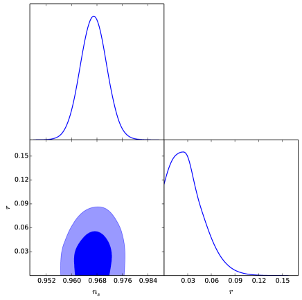
Figure 1: The marginalized contour plots and the likelihood distributions of $r$ and $n_{s}$ in the base $\Lambda$CDM+$r$ model.

The constraints on $r$ and $n_{s}$ are given by

$$r_{0.01}<0.0685~{}~{}(95\%~{}\textrm{C.L.})\ ,$$ (5)

$$n_{s}=0.9669\pm 0.0040~{}~{}(68\%~{}\textrm{C.L.})\ .$$ (6)

The primordial scalar power spectrum deviates from the Harrison-Zel’dovich spectrum at more than $8\sigma$ C.L..

The marginalized contour plots and the likelihood distributions of $r$, $n_{s}$ and $dn_{s}/d\ln k$ in the base $\Lambda$CDM+$r$+nrun model show up in Fig. 2.

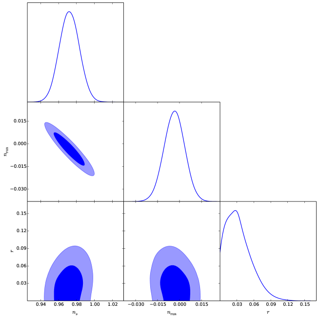
Figure 2: The marginalized contour plots and the likelihood distributions of $r$, $n_{s}$ and $n_{\textrm{run}}\equiv dn_{s}/d\ln k$ in the base $\Lambda$CDM+$r$+nrun model.

We see that the constraints on $r$, $n_{s}$ and $dn_{s}/d\ln k$ read

$$r_{0.01}<0.0751~{}~{}(95\%~{}\textrm{C.L.})\ ,$$ (7)

$$n_{s}=0.9721\pm 0.0108~{}~{}(68\%~{}\textrm{C.L.})\ ,$$ (8)

$$dn_{s}/d\ln k=-0.0035\pm 0.0068~{}~{}(68\%~{}\textrm{C.L.})\ .$$ (9)

Even though there is one more parameter in the $\Lambda$CDM+$r$+nrun model, the best-fit $\chi^{2}$ is the same as that in the $\Lambda$CDM+$r$ model. We conclude that P15+BK14+BAO15 data do not prefer a non-zero running of scalar spectral index from the statistic point of view.

Finally, the marginalized contour plots and the likelihood distributions of $r$, $n_{s}$, $dn_{s}/d\ln k$ and $d^{2}n_{s}/d\ln k^{2}$ in the base $\Lambda$CDM+$r$+nrun+nrunrun model are illustrated in Fig. 3.

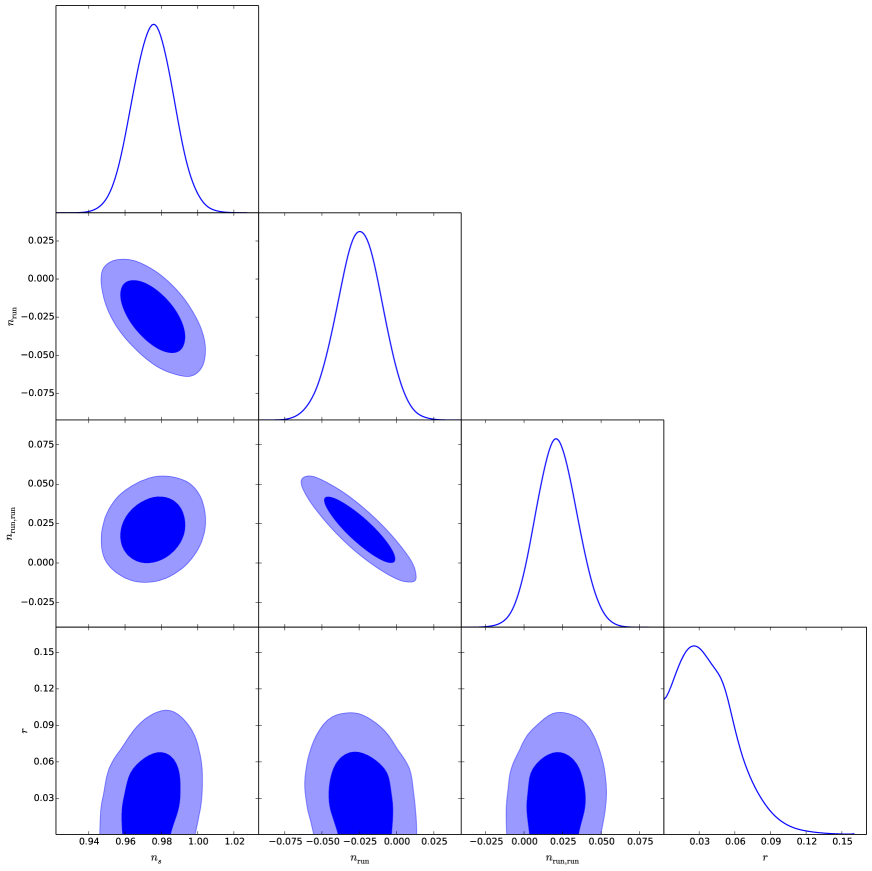
Figure 3: The marginalized contour plots and the likelihood distributions of $r$, $n_{s}$, $n_{\textrm{run}}\equiv dn_{s}/d\ln k$ and $n_{\textrm{run,run}}\equiv d^{2}n_{s}/d\ln k^{2}$ in the base $\Lambda$CDM+$r$+nrun+nrunrun model.

We see that the constraints on $r$, $n_{s}$, $dn_{s}/d\ln k$ and $d^{2}n_{s}/d\ln k^{2}$ are

$$r_{0.01}<0.0814~{}~{}(95\%~{}\textrm{C.L.})\ ,$$ (10)

$$n_{s}=0.9756\pm 0.0111~{}~{}(68\%~{}\textrm{C.L.})\ ,$$ (11)

$$dn_{s}/d\ln k=-0.0247\pm 0.0148~{}~{}(68\%~{}\textrm{C.L.})\ ,$$ (12)

$$d^{2}n_{s}/d\ln k^{2}=0.0211\pm 0.0130~{}~{}(68\%~{}\textrm{C.L.})\ .$$ (13)

Our results show a slight preference for the negative running and a positive running of running of the scalar spectral index at the pivot scale $k_{p}=0.01$ Mpc^-1, and $\Delta\chi^{2}\simeq-3.3$ compared to the base $\Lambda$CDM+$r$ model.

III Constraints on inflation

The equations of motion for the canonical single-field slow-roll inflation take the form

$$H^{2} = {1\over 3M_{p}^{2}}\left[{1\over 2}{\dot{\phi}}^{2}+V(\phi)\right],$$ (14)

$$\ddot{\phi} + 3H\dot{\phi}+V^{\prime}(\phi)=0,$$ (15)

where $M_{p}=1/\sqrt{8\pi G}$ is the reduced Planck energy scale, the dot and prime denote the derivative with respect to the cosmic time $t$ and the inflaton field $\phi$, respectively. The inflaton field slowly rolls down its potential if $\epsilon\ll 1$ and $|\eta|\ll 1$, where

$$\epsilon \equiv {M_{p}^{2}\over 2}\left({V^{\prime}\over V}\right)^{2},$$ (16)

$$\eta \equiv M_{p}^{2}{V^{\prime\prime}\over V}.$$ (17)

In this limit, the equations of motion are simplified to

$$H^{2} \simeq {V(\phi)\over 3M_{p}^{2}},$$ (18)

$$3H\dot{\phi} \simeq -V^{\prime}(\phi).$$ (19)

From the dynamics of inflation, we have

$$\eta=2\epsilon+{1\over 2}{d\ln\epsilon\over dN},$$ (20)

where $N\equiv\int_{t}^{t_{\rm end}}H(t^{\prime})dt^{\prime}$ is the number of e-folds before the end of inflation. The amplitudes of scalar and tensor power spectra are respectively given by

$$P_{s} = {V\over 24\pi^{2}M_{p}^{2}\epsilon},$$ (21)

$$P_{t} = {2V\over 3\pi^{2}M_{p}^{2}}.$$ (22)

Therefore the tensor-to-scalar ratio and the spectral index of scalar power spectrum are related to the slow-roll parameters by

$$r = 16\epsilon,$$ (23)

$$n_{s} = 1-6\epsilon+2\eta.$$ (24)

See, for example, Huang:2014yaa in detail.

III.1 Selection of inflation models

There are a large number of inflation models in the market Martin:2013tda . It is almost impossible to figure out a unique inflation model even when the cosmological parameters are measured very accurately, because the number of the cosmological parameters we can measure should be limited. In general, the simplicity is considered as a basic principle we should follow. In this subsection, we only take into account a few simple inflation models and compare them with the global fitting results given in the former section. Our main results are illustrated in Fig. 4. At first glance, we see that the inflation model with a concave potential is preferred at around $95\%$ C.L..

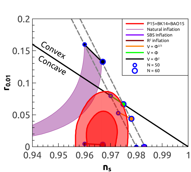
Figure 4: Comparing the inflation models with the observational constraints.

The inflation model with a monomial potential $V(\phi)\sim\phi^{n}$ Linde:1983gd is the simplest class of inflation models, and is the prototype of chaotic inflation model. The predictions of this model are

$$r = \frac{14n}{N},$$ (25)

$$n_{s} = 1-\frac{n+2}{2N}.$$ (26)

Here $n$ is not necessarily an integer. Axion monodromy was supposed to achieve $V(\phi)\sim\phi^{n}$ inflation model in string theory. For example, $n=2/5$, $2/3$ in Silverstein:2008sg , $n=1$ in McAllister:2008hb , and the models with higher power in Marchesano:2014mla ; McAllister:2014mpa . For $50<N<60$, the predictions of $V(\phi)\sim\phi^{n}$ inflation model are illustrated in the region between two grey dashed lines in Fig. 4. Unfortunately, we see that this class of inflation models are marginally disfavored at around $95\%$ C.L..

In the natural inflation model Freese:1990rb ; Adams:1992bn , the effective one-dimensional potential is given by $V(\phi)=m^{2}f^{2}\left(1+\cos(\phi/f)\right)$ where $f$ denotes the decay constant. The natural inflation predicts

$$r = \frac{8}{(f/M_{p})^{2}}\frac{1+\cos\theta_{N}}{1-\cos\theta_{N}},$$ (27)

$$n_{s} = 1-\frac{1}{(f/M_{p})^{2}}\frac{3+\cos\theta_{N}}{1-\cos\theta_{N}},$$ (28)

where

$$\cos\frac{\theta_{N}}{2}=\exp\left(-\frac{N}{2(f/M_{p})^{2}}\right)\ .$$ (29)

For $50<N<60$, the different decay constant corresponds to different predictions. See the purple shaded region in Fig. 4. Compared to the constraints from data, the natural inflation model is also marginally disfavored at $95\%$ C.L..

In the spontaneously broken SUSY (SBS) inflation model SUSY , the potential of inflaton field takes the form of $V(\phi)=V_{0}\left(1+c\ln\frac{\phi}{Q}\right)$ where $V_{0}$ is dominant and $c<<1$. This inflation model predicts

$$r \simeq 0,$$ (30)

$$n_{s} = 1-\frac{1}{N}.$$ (31)

It is also disfavored at more than $95\%$ C.L., because it predicts a large scalar spectral index. If the soft SUSY breaking term is taken into account, the scalar spectral index can shift to fit the data Rehman:2009nq ; Pallis:2013dxa .

In the Starobinsky inflation model Starobinsky:1980te , the inflationary expansion of the Universe is driven by a higher derivative term in the action, namely $S=\frac{M_{p}^{2}}{2}\int d^{4}x\sqrt{-g}\left(R+\frac{R^{2}}{6M^{2}}\right)$ where $M$ denotes an energy scale. The tensor-to-scalar ratio and the scalar spectral index in Starobinsky inflation model are given by

$$r \simeq \frac{12}{N^{2}},$$ (32)

$$n_{s} = 1-\frac{2}{N},$$ (33)

in Mukhanov:1981xt ; Starobinsky:1983zz . Even though this inflation model can fit the data quite well, why the terms with higher powers of $R$ are all suppressed Huang:2013hsb is still an open question.

III.2 Constraints on typical inflation models

In this subsection, we propose a new method to explore the space of inflation models. Similar to Huang:2007qz , we parametrize the slow-roll parameter $\epsilon(N)$ in terms of e-folding number $N$ for the typical inflation model as follows

$$\epsilon(N)={c/2\over(N+\Delta N)^{p}},$$ (34)

where $c(>0)$ and $p$ are two constants, and

$$\Delta N=\left({c\over 2}\right)^{1/p}.$$ (35)

Here we introduce $\Delta N$ to keep $N=0$ at the end of inflation, namely $\epsilon(N=0)=1$. See some extended investigations in Mukhanov:2013tua ; Roest:2013fha ; Garcia-Bellido:2014wfa ; Gobbetti:2015cya . Now the tensor-to-scalar ratio reads

$$r={8c\over(N+\Delta N)^{p}}.$$ (36)

From Eq. (20), we obtain

$$\eta = {c\over(N+\Delta N)^{p}}-{p\over 2(N+\Delta N)},$$ (37)

and then

$$n_{s}=1-{c\over(N+\Delta N)^{p}}-{p\over N+\Delta N}.$$ (38)

Even though this parametrization can not cover all of the canonical single-field slow-roll inflation models, it can really cover many well-known inflation models.
$\bullet$ For the inflation model with $V(\phi)\sim\phi^{n}$, we have $p=1$ and $c=n/2$.
$\bullet$ For the Starobinsky model, we have $p=2$ and $c=3/2$.
$\bullet$ For the brane inflation model Dvali:1998pa with $V(\phi)=V_{0}(1-(\mu/\phi)^{d-2})$, we have $p=2(d-1)/d$, where $d$ is the number of transverse dimensions. For example, the D3-Brane inflation in the KKLMMT setup predicts $p=5/3$ and $c\simeq 0$ Kachru:2003sx .

Up to now the exact e-folding number corresponds to the pivot scale $k_{p}$ is still unknown. Usually it is considered to be a number between 50 and 60. In this subsection, we take $N$ as a free parameter. Adopting the flat priors for $c\in[0,100]$, $p\in[0.5,3]$ and $N\in[50,60]$, globally fitting P15+BK14+BAO data combination and finally marginalizing over other free parameters in the base $\Lambda$CDM model and $N$, we obtain the constraints on the parameters $c$ and $p$, namely

$$p = 2.07_{-0.28}^{+0.32}\quad(68\%\ \textrm{C.L.}),$$ (39)

$$c < 65.7\quad(95\%\ \textrm{C.L.}).$$ (40)

See Fig. 5 as well.

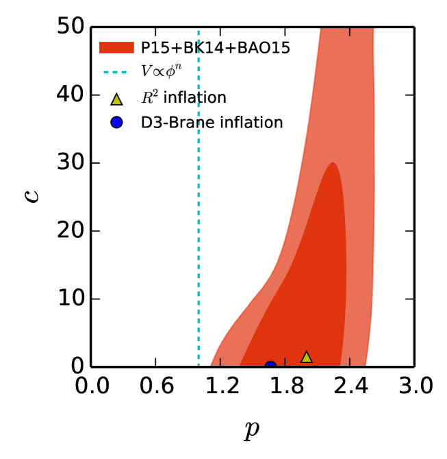
Figure 5: Constraints on the space of inflation models from P15+BK14+BAO15.

We see that the inflation model with a monomial potential corresponds to $p=1$ which is disfavored at more than $95\%$ C.L.. But both the Brane inflation model and the Starobinsky inflation model still fit the data quite well.

IV Summary and Discussion

In this paper, we constrained the cosmological parameters in the base $\Lambda$CDM+$r$ model and two extended models by jointly analyzing the data combination including Planck 2015 data of CMB anisotropies and polarizations as well as CMB lensing, BICEP2 & Keck Array data of B-mode polarization up to and including 2014 observing season, and the anisotropic BAO distance scales from SDSS-III BOSS DR12 together with the isotropic 6dFGS and MGS BAO data. Comparing with the predictions of inflation models, we find that the inflation model with a concave potential is preferred and both the inflation model with a monomial potential and the natural inflation model are marginally disfavored at $95\%$ C.L.. But both the Brane inflation model and the Starobinsky inflation model still give a good fit to the current data.

Even though there is no evidence for supporting a non-zero running of scalar spectral index, a positive running of running in order of ${\cal O}(10^{-2})$ provides a slightly better fit to the data. Such a positive running of running can significantly relax the Lyth bound on the tensor-to-scalar ratio to $0.1$ Huang:2015xda .

Before closing this paper, we also want to sketch the potential of inflaton field according to the current cosmological data. To summarize, the preferred inflation potential goes like that as follows

$$V(\phi)=\Lambda_{*}-\delta V(\phi),$$ (41)

where $\Lambda_{*}$ is an effective cosmological constant which determines the energy scale of inflation, and the dynamics of inflation is described by the subdominant term $\delta V(\phi)$. Since the concave shape of potential is preferred, $\delta V^{\prime\prime}(\phi)>0$. For example, for

$$V(\phi)=\Lambda_{*}\left[1-\left({\phi\over\mu}\right)^{n}\right],$$ (42)

where $\mu$ is an energy scale, $n$ is related to $p$ in Eq. (34) by

$$n={2(p-1)\over p-2}\quad\hbox{for}\ p>1\ \hbox{and}\ p\neq 2.$$ (43)

Note that $p=2$ corresponds $V(\phi)=\Lambda_{*}\left[1-\exp(-{\phi/\mu})\right]$. From Sec. III.2, we find $p>1$ which implies $n<0$ or $n>2$ and the potential is certainly concave. Now we still cannot distinguish the sign of $n$. We hope that the accurate experiments will tell us more detail about inflation in the near future.

Acknowledgments We acknowledge the use of HPC Cluster of SKLTP/ITP-CAS. This work is supported by Top-Notch Young Talents Program of China and grants from NSFC (grant NO. 11322545, 11335012 and 11575271). QGH would also like to thank the participants of the advanced workshop “Dark Energy and Fundamental Theory” supported by the Special Fund for Theoretical Physics from the National Natural Science Foundations of China (grant No. 11447613) for useful conversation.

References

- (1) A. A. Starobinsky, Phys. Lett. B 91, 99 (1980).
- (2) A. H. Guth, Phys. Rev. D 23, 347 (1981).
- (3) A. D. Linde, Phys. Lett. B 108, 389 (1982).
- (4) A. Albrecht and P. J. Steinhardt, Phys. Rev. Lett. 48, 1220 (1982).
- (5) R. Adam et al. [Planck Collaboration], arXiv:1502.01582 [astro-ph.CO].
- (6) P. A. R. Ade et al. [Planck Collaboration], arXiv:1502.02114 [astro-ph.CO].
- (7) P. A. R. Ade et al. [BICEP2 Collaboration], Phys. Rev. Lett. 112, 241101 (2014) [arXiv:1403.3985 [astro-ph.CO]].
- (8) M. J. Mortonson and U. Seljak, JCAP 1410, 035 (2014) [arXiv:1405.5857 [astro-ph.CO]].
- (9) R. Flauger, J. C. Hill and D. N. Spergel, JCAP 1408, 039 (2014) [arXiv:1405.7351 [astro-ph.CO]].
- (10) R. Adam et al. [Planck Collaboration], arXiv:1409.5738 [astro-ph.CO].
- (11) C. Cheng, Q. G. Huang and S. Wang, JCAP 1412, no. 12, 044 (2014) [arXiv:1409.7025 [astro-ph.CO]].
- (12) P. A. R. Ade et al. [BICEP2 and Planck Collaborations], Phys. Rev. Lett. 114, 101301 (2015) [arXiv:1502.00612 [astro-ph.CO]].
- (13) P. A. R. Ade et al. [BICEP2 and Keck Array Collaborations], arXiv:1510.09217 [astro-ph.CO].
- (14) A. J. Cuesta et al., arXiv:1509.06371 [astro-ph.CO].
- (15) H. Gil-Marin et al., arXiv:1509.06373 [astro-ph.CO].
- (16) F. Beutler et al., Mon. Not. Roy. Astron. Soc. 416, 3017 (2011) [arXiv:1106.3366 [astro-ph.CO]].
- (17) A. J. Ross, L. Samushia, C. Howlett, W. J. Percival, A. Burden and M. Manera, Mon. Not. Roy. Astron. Soc. 449, no. 1, 835 (2015) [arXiv:1409.3242 [astro-ph.CO]].
- (18) A. R. Liddle and D. H. Lyth, Phys. Lett. B 291, 391 (1992) [astro-ph/9208007].
- (19) C. Cheng and Q. G. Huang, Eur. Phys. J. C 74, no. 11, 3139 (2014) [arXiv:1403.7173 [astro-ph.CO]].
- (20) Q. G. Huang and S. Wang, JCAP 1506, no. 06, 021 (2015) [arXiv:1502.02541 [astro-ph.CO]].
- (21) G. Cabass, L. Pagano, L. Salvati, M. Gerbino, E. Giusarma and A. Melchiorri, arXiv:1511.05146 [astro-ph.CO].
- (22) Q. G. Huang, S. Wang and W. Zhao, JCAP 1510, no. 10, 035 (2015) [arXiv:1509.02676 [astro-ph.CO]].
- (23) A. Lewis, A. Challinor and A. Lasenby, Astrophys. J. 538, 473 (2000) [astro-ph/9911177].
- (24) C. Howlett, A. Lewis, A. Hall, and A. Challinor, JCAP 04, 027 (2012).
- (25) A. Lewis and S. Bridle, Phys. Rev. D 66, 103511 (2002) [astro-ph/0205436].
- (26) Q. G. Huang, Sci. China Phys. Mech. Astron. 58, no. 11, 110401 (2015) [arXiv:1407.4639 [astro-ph.CO]].
- (27) J. Martin, C. Ringeval and V. Vennin, Phys. Dark Univ. 5-6, 75 (2014) [arXiv:1303.3787 [astro-ph.CO]].
- (28) A. D. Linde, Phys. Lett. B 129, 177 (1983).
- (29) E. Silverstein and A. Westphal, Phys. Rev. D 78, 106003 (2008) [arXiv:0803.3085 [hep-th]].
- (30) L. McAllister, E. Silverstein and A. Westphal, Phys. Rev. D 82, 046003 (2010) [arXiv:0808.0706 [hep-th]].
- (31) F. Marchesano, G. Shiu and A. M. Uranga, JHEP 1409, 184 (2014) [arXiv:1404.3040 [hep-th]].
- (32) L. McAllister, E. Silverstein, A. Westphal and T. Wrase, JHEP 1409, 123 (2014) [arXiv:1405.3652 [hep-th]].
- (33) K. Freese, J. A. Frieman and A. V. Olinto, Phys. Rev. Lett. 65, 3233 (1990).
- (34) F. C. Adams, J. R. Bond, K. Freese, J. A. Frieman and A. V. Olinto, Phys. Rev. D 47, 426 (1993) [hep-ph/9207245].
- (35) G. R. Dvali, Q. Shafi and R. K. Schaefer, Phys. Rev. Lett. 73, 1886 (1994) [hep-ph/9406319]; E. J. Copeland, A. R. Liddle, D. H. Lyth, E. D. Stewart and D. Wands, Phys. Rev. D 49, 6410 (1994); P. Binetruy and G. R. Dvali, Phys. Lett. B 388, 241 (1996) [hep-ph/9606342]; E. D. Stewart, Phys. Rev. D 51, 6847 (1995) [hep-ph/9405389]; D. H. Lyth and A. Riotto, Phys. Rept. 314, 1 (1999) [hep-ph/9807278].
- (36) M. U. Rehman, Q. Shafi and J. R. Wickman, Phys. Lett. B 683, 191 (2010) [arXiv:0908.3896 [hep-ph]].
- (37) C. Pallis and Q. Shafi, Phys. Lett. B 725, 327 (2013) [arXiv:1304.5202 [hep-ph]].
- (38) V. F. Mukhanov and G. V. Chibisov, JETP Lett. 33, 532 (1981) [Pisma Zh. Eksp. Teor. Fiz. 33, 549 (1981)].
- (39) A. A. Starobinsky, Sov. Astron. Lett. 9, 302 (1983).
- (40) Q. G. Huang, JCAP 1402, 035 (2014) [arXiv:1309.3514 [hep-th]].
- (41) Q. G. Huang, Phys. Rev. D 76, 061303 (2007) [arXiv:0706.2215 [hep-th]].
- (42) V. Mukhanov, Eur. Phys. J. C 73, 2486 (2013) [arXiv:1303.3925 [astro-ph.CO]].
- (43) D. Roest, JCAP 1401, 007 (2014) [arXiv:1309.1285 [hep-th]].
- (44) J. Garcia-Bellido, D. Roest, M. Scalisi and I. Zavala, Phys. Rev. D 90, no. 12, 123539 (2014) [arXiv:1408.6839 [hep-th]].
- (45) R. Gobbetti, E. Pajer and D. Roest, JCAP 1509, no. 09, 058 (2015) [arXiv:1505.00968 [astro-ph.CO]].
- (46) G. R. Dvali and S. H. H. Tye, Phys. Lett. B 450, 72 (1999) [hep-ph/9812483].
- (47) S. Kachru, R. Kallosh, A. D. Linde, J. M. Maldacena, L. P. McAllister and S. P. Trivedi, JCAP 0310, 013 (2003) [hep-th/0308055].
- (48) Q. G. Huang, Phys. Rev. D 91, no. 12, 123532 (2015) [arXiv:1503.04513 [astro-ph.CO]].