Computing Chebyshev knot diagrams

Abstract

A Chebyshev curve ${\cal C}(a,b,c,\varphi)$ has a parametrization of the form $x(t)=T_{a}(t)$;   $y(t)=T_{b}(t)$; $z(t)=T_{c}(t+\varphi)$, where $a,b,c$ are integers, $T_{n}(t)$ is the Chebyshev polynomial of degree $n$ and $\varphi\in{\bf R}$. When ${\cal C}(a,b,c,\varphi)$ is nonsingular, it defines a polynomial knot. We determine all possible knot diagrams when $\varphi$ varies. Let $a,b,c$ be integers, $a$ is odd, $(a,b)=1$, we show that one can list all possible knots ${\cal C}(a,b,c,\varphi)$ in $\widetilde{\mathcal{O}}(n^{2})$ bit operations, with $n=abc$.

Keywords: Zero dimensional systems, Chebyshev curves, Lissajous knots, polynomial knots, factorization of Chebyshev polynomials, minimal polynomial, Chebyshev forms.

1 Introduction

It is known that every knot in $\SS^{3}$ can be represented as the closure of the image of a polynomial embedding ${\bf R}\to{\bf R}^{3}\subset\SS^{3}$, see Vassiliev (1990). Given a knot $K$, it is in general a difficult problem to determine $(a,b,c)$ such that there exists a polynomial embedding ${\bf R}\to{\bf R}^{3}$ of multi-degree $(a,b,c)$ that parametrizes $K$ and an even more difficult problem to determine a minimal $(a,b,c)$, for the lexicographic ordering, see for example (Brugallé, Koseleff, and Pecker, 2016).

A Chebyshev curve ${\cal C}(a,b,c,\varphi)$ is the space curve

$${\cal C}(a,b,c,\varphi):x=T_{a}(t),\,y=T_{b}(t),\,z=T_{c}(t+\varphi),$$

where $T_{n}(x)=2\cos(n\arccos x/2)$ is the monic Chebyshev polynomial of degree $n$, $a$, $b$, $c$ with $a,b$ coprime and $a<b$, are positive integers, and $\varphi$ is a real number. If a Chebyshev curve ${\cal C}(a,b,c,\varphi)$ is nonsingular, then it defines a (long) knot.

Chebyshev knots are polynomial analogues of Lissajous knots, which admit parametrizations of the form $x=\cos(at);y=\cos(bt+\varphi);z=\cos(ct+\psi)$. These knots were first introduced by Bogle, Hearst, Jones, and Stoilov (1994). It is known that every knot is not necessarily a Lissajous knot. Recently, it is shown in (Soret and Ville, 2016) that every knot is a Fourier knot, which admits a parametrization of the form $x=\cos(at);y=\cos(bt+\varphi);z=\lambda\cos(ct+\psi)+\lambda^{\prime}\cos(c^{\prime}t+\psi^{\prime})$.

In (Koseleff and Pecker, 2011), it is proved that every (long) knot $K\subset{\bf R}^{3}\subset\SS^{3}$ is a Chebyshev knot, that is to say there exists a Chebyshev curve ${\cal C}(a,b,c,\varphi)$ that is isotopic to $K$ in $\SS^{3}$.

The objective of our contribution is to compute minimal Chebyshev parametrization exhaustively for the first two-bridge knots with 10 crossings and fewer.

Our strategy consists in studying exhaustively Chebyshev curves with increasing degrees and identify the knots they represent. As every knot is a Chebyshev knot, this process will describe all the first knots as soon as we can identify each knot. To identify a knot, we compute its diagram and this computation is the core of the process.

1.1 Chebyshev Diagrams

To a space curve is associated its diagram, which is given by the projection on ${\bf R}^{2}$ and the (under/over) nature of the crossings. From a diagram one can compute several knot invariants that may allow to determine the corresponding knot. It is in general a difficult problem when the minimal number of crossings of the knot is greater than 16. We will not discuss this question in the present contribution.

If $a$ and $b$ are coprime integers, then the curve ${\cal C}(a,b,c,\varphi)$ is singular if and only if it has double points. Let us introduce the polynomials $P_{n}$ and $Q_{n}$ defined by

$$P_{n}(t,s)={\displaystyle{{T_{n}(t)-T_{n}(s)}\overwithdelims. .{t-s}}},\ Q_{n}(t,s,\varphi)={\displaystyle{{T_{n}(t+\varphi)-T_{n}(s+\varphi)}\overwithdelims. .{t-s}}}.$$ (1)

Then, ${\cal C}(a,b,c,\varphi)$ is a knot if and only if

$$\left\{(s,t),\,P_{a}(s,t)=P_{b}(s,t)=Q_{c}(s,t,\varphi)=0\right\}$$ (2)

is empty. The projection of the Chebyshev space curve ${\cal C}(a,b,c,\varphi)$ on the $xy$-plane is the plane Chebyshev curve

$${\cal C}(a,b):x=T_{a}(t);\,y=T_{b}(t).$$

The crossing points of ${\cal C}(a,b)$ lie on the $(b-1)$ vertical lines $T^{\prime}_{b}(x)=0$ and on the $(a-1)$ horizontal lines $T^{\prime}_{a}(y)=0$. We can represent the knot ${\cal C}(a,b,c,\varphi)$ by a billiard diagram (Koseleff and Pecker, 2011) which is a purely combinatorial object, see for example (Cohen and Krishnan, 2015). As an example, consider the knots $\overline{5}_{2}={\cal C}(4,5,7,0)$, ${5}_{2}={\cal C}(5,6,7,0)$, $\overline{4}_{1}={\cal C}(3,5,7,0)$ in Figure 1.

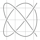
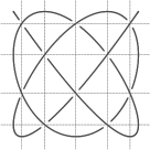
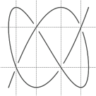
$\overline{5}_{2}$	${5}_{2}$	$\overline{4}_{1}$

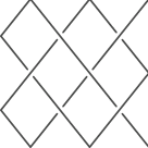
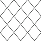
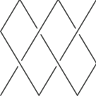
Figure 1: Some Chebyshev knot diagrams and their billiard trajectories

There are two kinds of crossing: the right twist and the left twist, see (Murasugi, 2007) and Figure 2.

Figure 2: The right twist and the left twist

In (Koseleff et al., 2010, Lemma 6), it is shown that ${\cal C}(a,b)$ has $(a-1)(b-1)/2$ double points $A_{\alpha,\beta}$ corresponding to parameters ($t=2\cos(\alpha+\beta),s=2\cos(\alpha-\beta)$, $\alpha={\textstyle{{i\pi}\overwithdelims. .{a}}}$, $\beta={\textstyle{{j\pi}\overwithdelims. .{b}}}$) and the nature of the crossing over $A_{\alpha,\beta}$ is given by the sign of

$$D(s,t,\varphi)=Q_{c}(s,t,\varphi)P_{b-a}(s,t)=(-1)^{i+j+\lfloor{{\textstyle{{ib}\overwithdelims. .{a}}}}\rfloor+\lfloor{{\textstyle{{ja}\overwithdelims. .{b}}}}\rfloor}Q_{c}(s,t,\varphi).$$ (3)

1.2 The discriminant polynomial

If $(a,b)=1$, then the algebraic set

$${\cal V}_{a,b}=\{(s,t)\in{\bf C}^{2},\,P_{a}(s,t)=P_{b}(s,t)=0\}$$

has exactly $(a-1)(b-1)$ points, and they are real (Koseleff and Pecker, 2011). The leading coefficient of $Q_{c}$, viewed as a univariate polynomial in $\varphi$, is equal to $c$ and then

$${\cal V}_{a,b,c}=\left\{(s,t,\varphi)\in{\bf C}^{3},P_{a}(s,t)=P_{b}(s,t)=Q_{c}(s,t,\varphi)=0\right\}$$

is also a finite set of complex points (see Koseleff et al. (2010, Prop. 5)). The projection

$${\cal Z}_{a,b,c}=\{\varphi\in{\bf C}\,|\,\exists(s,t),\,P_{a}(s,t)=P_{b}(s,t)=Q_{c}(s,t,\varphi)=0\}$$

is also a finite number of points which discriminates the possible knots: if the interval $(\varphi_{1},\varphi_{2})$ does not intersect ${\cal Z}_{a,b,c}$, then ${{\cal C}}(a,b,c,\varphi_{1})$ and ${{\cal C}}(a,b,c,\varphi_{2})$ represent the same knot, because the nature of their crossings (in Formula 3) does not change.

One can consider ${\cal Z}_{a,b,c}$ as the zero set of $\langle\tilde{R}_{a,b,c}\rangle=\langle P_{a},P_{b},Q_{c}\rangle\cap{\bf Q}[\varphi]$ or as the zero set of the characteristic polynomial $\hat{R}_{a,b,c}$ of $\varphi$ in ${\bf Q}[s,t,\varphi]\bigm{/}\langle P_{a},P_{b},Q_{c}\rangle$ which both are polynomials with rational coefficients that could be computed using classical elimination tools, see Koseleff, Pecker, and Rouillier (2010), for example by computing a Gröbner basis for any elimination order with $\varphi<s,t$ or by performing linear algebra in ${\bf Q}[s,t,\varphi]\bigm{/}\langle P_{a},P_{b},Q_{c}\rangle$.

The information about the multiplicities of the points of ${\cal Z}_{a,b,c}$ viewed as roots of $\tilde{R}_{a,b,c}$ or $\hat{R}_{a,b,c}$ is useless so, in this contribution, we will define $R_{a,b,c}$ as a polynomial (of degree ${\textstyle{{1}\overwithdelims. .{2}}}(a-1)(b-1)(c-1)$) with the same roots as $\tilde{R}_{a,b,c}$ or $\hat{R}_{a,b,c}$ and we will name it the discriminant polynomial (for a fixed $(a,b,c)$).

1.3 Motivations

In (Boocher, Daigle, Hoste, and Zheng, 2009), Lissajous knots have been sampled by numerical experiments, and several knots with relatively small crossing numbers were identified.

Given $a,b,c$ integers, $a,b$ coprime, and $\varphi$ a rational number, our first goal is

1. decide if ${\cal C}(a,b,c,\varphi)$ is singular;

2. if not, determine its diagram, that is the sign of $D(s,t,\varphi)$ for all $(s,t)$ in ${\cal V}_{a,b}$.

Given $a,b,c$ integers, $a,b$ coprime, our second goal is to determine all possible diagrams corresponding to a knot ${\cal C}(a,b,c,\varphi)$.

1. compute the discriminant polynomial $R_{a,b,c}(\varphi)$ (or any polynomial with the same roots as $\tilde{R}_{a,b,c}$ such that $\langle\tilde{R}_{a,b,c}\rangle=\langle P_{a},P_{b},Q_{c}\rangle\cap Q[\varphi]$);

2. compute the real roots $\varphi_{1}<\cdots<\varphi_{s}$ of $R_{a,b,c}(\varphi)$;

3. for an arbitrary set of rational numbers $r_{0}<\varphi_{1}<r_{1}<\varphi_{2}<\cdots<r_{s-1}<\varphi_{s}<r_{s}$, compute the $xy$-diagrams of ${\cal C}(a,b,c,r_{i})$.

In (Koseleff et al., 2010), the study of Chebyshev knots ${\cal C}(a,b,c,\varphi)$ was restricted to the case $a\leq 4$, corresponding to two-bridge knots. In this case the knots were easily deduced from their diagrams, by computing the Schubert fraction, see (Murasugi, 2007).

The discriminant polynomial $R_{a,b,c}$ was directly obtained as a (product of) resultant(s) with integer coefficients. The method in (Koseleff et al., 2010) was essentially based on usual general black-boxes for solving the zero-dimensional system

$$\left\{P_{a}(s,t)=P_{b}(s,t)=Q_{c}(s,t,\varphi)=T-D(s,t,\varphi)=0\right\},$$

for example by computing a rational univariate representation (RUR, see Rouillier (1999)) of its zeroes and then compute the sign of the $T$-coordinate of each real root.

In (Koseleff et al., 2010) an exhaustive list of minimal parametrization was obtained for all (but six) two-bridge knots with 10 and fewer crossings, by enumerating all possible diagrams ${\cal C}(a,b,c,\varphi)$, for increasing $a<b<c$. For these six knots one could not find any integer $c$ nor any rational number $\varphi$, such that ${\cal C}(a,b,c,\varphi)$ was a parametrization. One of the reason was that the discriminant polynomial $R_{a,b,c,}$ was too difficult to compute using classical elimination techniques.

In the present paper, we are not limited to the case $a\leq 4$ anymore and thus, in addition to the description of the algorithms used, it makes sense to analyse their complexity.

We rather use some remarkable properties of the implicit Chebyshev curves to factorize the discriminant polynomial over the real cyclotomic extension ${\bf Q}[2\cos\pi/n]$, (where $n\leq abc$). We thus completely change the computational strategy: one has now to deal with univariate polynomials of low degrees but with coefficients in some field extensions of high degrees.

We make use of specific properties of Chebyshev polynomials as well as specific algorithms (Koseleff, Rouillier, and Tran, 2015) working in the Chebyshev basis instead of the usual monomial basis to speed up dramatically the computations. This new modelization and the related algorithms allow us to obtain all the classifications of (Koseleff et al., 2010) in a few minutes, including the six knots that where not reached.

1.4 Contents of this paper

In Section 2, we recall some basic properties of Chebyshev polynomials and then give geometric properties of Lissajous and Chebyshev curves. We propose a factorization of $T_{m}(x)-T_{m^{\prime}}(y)$. The particular case $m^{\prime}=m$ is used to factorize $R_{a,b,c}$ and isolate its real roots. Note that this factorisation is also used in (Dimca and Sticlaru, 2012) in a much more theoretical context.

Section 3 is devoted to the computation of $R_{a,b,c}$. We propose a factorization in ${\bf Z}[\varphi]$ as well as in ${\bf Z}[2\cos\pi/n][\varphi]$ with $n=abc$. We then study two different ways for computing $R_{a,b,c}$: expressing $R_{a,b,c}$ in ${\bf Z}[2\cos\pi/n][\varphi]$ as a Chebyshev form or by certified and accurate numerical approximations. In the first case, we evaluate to $\widetilde{\mathcal{O}}(n^{4})$ bit operations the cost of the computation, which outperforms the time required by a straightforward method based on Gröbner bases or resultants and in the second case, we show that the computation requires only $\widetilde{\mathcal{O}}(n^{3})$ bit operations. All these results are based on results on the cyclotomic extension ${\bf Z}[2\cos\pi/n]$ that have been recently published in (Koseleff et al., 2015).

In Section 4, we focus on the isolation of the real roots of $R_{a,b,c}$. We first show that the coefficients of $R_{a,b,c}$ are all bounded in absolute value by $6^{N}$, with $N={\textstyle{{1}\overwithdelims. .{2}}}(a-1)(b-1)(c-1)$ so a direct method using state-of-the-art algorithms would isolate the real roots in $\widetilde{\mathcal{O}}(n^{3})$ bit operations. We then propose an ad-hoc method that computes the real roots in $\widetilde{\mathcal{O}}(n^{2})$ bit operations, thanks to a good separation of the roots ($>2^{-8n}$). This method does not require to know explicitly the coefficients of $R_{a,b,c}$.

In Section 5, we propose some tools for computing all the possible knot diagrams ${\cal C}(a,b,c,\varphi)$ when $a,b,c\in{\bf Z}$, $a,b$ coprime, are fixed. We show that all the possible knot diagrams ${\cal C}(a,b,c,\varphi)$ can be listed in $\widetilde{\mathcal{O}}(n^{2})$ bit operations. We also show that given $\varphi\in{\bf Q}$ of bitsize $\tau$, it requires $\widetilde{\mathcal{O}}(n^{2}+n\tau)$ bit operations in order to decide if ${\cal C}(a,b,c,\varphi)$ is a knot and if so, $\widetilde{\mathcal{O}}(n^{2}\tau)$ bit operations to compute the nature of its crossings.

In the last section, we report the computation we performed to obtain all two-bridge knots with 10 crossings and fewer.

2 Chebyshev and Lissajous curves

In this section, we show that the implicit Chebyshev curve $T_{b}(x)=T_{a}(y)$ factorizes in Lissajous curves, which allows us to give explicit factorizations for $P_{a},P_{b}$ and $Q_{c}$ that will intensively be used in the sequel.

Chebyshev polynomials and their algebraic properties play a central role. The monic Chebyshev polynomials of the first kind, also called Dickson polynomials, are defined by the second-order linear recurrence

$$T_{0}=2,\,T_{1}=t,\,T_{n+1}=tT_{n}-T_{n-1}.$$ (4)

They satisfy the identity $T_{n}(2\cos\theta)=2\cos n\theta$, and then $T_{n}\circ T_{m}=T_{nm}$. The monic Chebyshev polynomials of the second kind satisfy $V_{n}(2\cos\theta)={\displaystyle{{\sin n\theta}\overwithdelims. .{\sin\theta}}}$ and $T^{\prime}_{n}=nV_{n}$. Both $T_{n}(t)$ and $V_{n}(t)$ belong to ${\bf Z}[t]$ and we have

$$T_{n}=\mathop{\prod}\limits_{k=0}^{n-1}(t-2\cos{\textstyle{{(2k+1)\pi}\overwithdelims. .{2n}}}),\quad V_{n}=\mathop{\prod}\limits_{k=1}^{n-1}(t-2\cos{\textstyle{{k\pi}\overwithdelims. .{n}}}).$$

The following classical properties will be useful in this section:

Lemma 2.1.

Let $T_{n}$ be the monic Chebyshev polynomial of the first kind.

• If $T^{\prime}_{n}(t)=0$ then $T_{n}(t)=\pm 2$, if $T_{n}(t)=\pm 2$ then $T^{\prime}_{n}(t)=0$ or $t=\pm 2$.

• $T_{n}(t)=y$ has $n$ real solutions if and only if $\left|y\right|<2$. $T_{n}(t)=2$ has $\lfloor{{\textstyle{{n}\overwithdelims. .{2}}}}\rfloor$ real solutions. $T_{n}(t)=-2$ has $\lfloor{{\textstyle{{n-1}\overwithdelims. .{2}}}}\rfloor$ real solutions.

Proof. From $T^{\prime}_{n}=nV_{n}$, we deduce that $t\mapsto T_{n}(t)$ is monotonic when $\left|t\right|\geq 2\cos{\textstyle{{\pi}\overwithdelims. .{n}}}$ and that $T_{n}$ has $n-1$ local extrema for $t_{k}=2\cos{\textstyle{{k\pi}\overwithdelims. .{n}}}$ where $T_{n}(t_{k})=2(-1)^{k}$. $\Box$

The following proposition gives a unified definition of Lissajous and Chebyshev curves:

Proposition 2.2.

Let $a,b$ be coprime integers ($a$ odd) and $\varphi\in{\bf R}$. The parametric curve

$${\cal C}:x=2\cos(at),\,y=2\cos(bt+\varphi),\,t\in{\bf C},$$

admits the equation $C_{a,b,\varphi}=0$ where

$$C_{a,b,\varphi}=T_{b}(x)^{2}+T_{a}(y)^{2}-2\cos(a\varphi)T_{b}(x)T_{a}(y)-4\sin^{2}(a\varphi).$$ (5)

1. If $a\varphi\not=k\pi$, then $C_{a,b,\varphi}$ is irreducible. ${\cal C}$ is called a Lissajous curve. Its real part is one-to-one parametrized for $t\in[0,2\pi]$.

2. If $a\varphi=k\pi$, then $C_{a,b,\varphi}=\bigl{(}T_{b}(x)-(-1)^{k}T_{a}(y)\bigr{)}^{2}$. ${\cal C}$ is called a Chebyshev curve. It can be one-to-one parametrized by $x=T_{a}(t),\,y=(-1)^{k}T_{b}(t)$.

Proof. Let $(x,y)\in{\cal C}$. We have $T_{b}(x)=2\cos(ab\,t),\,T_{a}(y)=2\cos(ab\,t+a\varphi)$. Let $\lambda=a\varphi,\,\theta=abt$. We get $T_{a}(y)=2\cos(\theta+\lambda)$ so $4(1-\cos^{2}\theta)\sin^{2}\lambda=(2\cos\theta\cos\lambda-T_{a}(y))^{2}$, that is $(4-T_{b}^{2}(x))\sin^{2}\lambda=(T_{b}(x)\cos\lambda-T_{a}(y))^{2},$ and we deduce our Equation (5).

Conversely, suppose that $(x,y)$ satisfies (5). Let $x=2\cos(at)$ where $t\in{\bf C}$. We also have $x=2\cos a(t+{\textstyle{{2k\pi}\overwithdelims. .{a}}})$ and $T_{b}(x)=2\cos\theta$. $A=T_{a}(y)$ is solution of the second-degree equation

$$A^{2}-2\,A\,\cos(a\varphi)\cos\theta-4\sin^{2}(a\varphi)=0.$$

Consequently, we get $T_{a}(y)=2\cos(\theta\pm a\varphi)=T_{a}(\cos(\pm bt+\varphi))$. We deduce that $y=2\cos(\pm bt+\varphi+{\textstyle{{2h\pi}\overwithdelims. .{a}}})$, $h\in{\bf Z}$. Changing $t$ by $-t$, we can suppose that

$$x=2\cos at,\,y=2\cos(bt+\varphi+{\textstyle{{2h\pi}\overwithdelims. .{a}}}).$$

By choosing $k$ such that $kb+h\equiv 0\,(\hbox{\rm mod}\,a)$, we get $x=2\cos at^{\prime},\,y=2\cos(bt^{\prime}+\varphi),$ where $t^{\prime}=t+{\textstyle{{2k\pi}\overwithdelims. .{a}}}$.

If $a\varphi\not\equiv 0\,(\hbox{\rm mod}\,\pi)$. Suppose that Equation (5) factors in $P(x,y)Q(x,y)$. We can suppose, for analyticity reasons, that $P(2\cos(at),2\cos(bt+\varphi))=0$, for $t\in{\bf C}$. The curve ${\cal C}$ intersects the line $y=0$ in $2b$ distinct points so $\deg_{x}P\geq 2b$. Similarly, $\deg_{y}P\geq 2a$ so that $Q$ is a constant which proves that the equation is irreducible.

If $\cos a\varphi=(-1)^{k}$, the equation becomes $T_{b}(x)-(-1)^{k}T_{a}(y)=0$. In this case the curve admits the announced parametrization, see (Fisher, 2001) and (Koseleff and Pecker, 2011) for more details. $\Box$

Definition 2.3.

Let $E_{\mu}(x,y)=x^{2}+y^{2}-2\cos(\mu)xy-4\sin^{2}(\mu)$ when $\mu\not\equiv 0\,(\hbox{\rm mod}\,\pi)$ and $E_{0}=x-y$, $E_{\pi}=x+y$. Equation (5) is equivalent to $E_{a\varphi}(T_{b}(x),T_{a}(y))=0$.

Remark 2.4.

If $a=b=1$, we obtain the Lissajous ellipses. They are the first curves studied by Lissajous (Lissajous, 1857). Let $\mu\not\equiv 0\,(\hbox{\rm mod}\,\pi).$ The curve $E_{\mu}(x,y)=0$ is an ellipse ${\cal E}_{\mu}$ inscribed in the square $[-2,2]^{2}$. It admits the parametrization $x=2\cos t,\,y=2\cos(t+\mu)$. This shows that the real part of the curve ${\cal C}$ (Equation (5)) is inscribed in the square $[-2,2]^{2}$.

$a=b=1,\varphi=\pi/3$	$a=2,b=3,\varphi=\pi/3$	$a=3,b=5,\varphi=2\pi/15$

Figure 3: Lissajous curves $x=2\cos at,y=2\cos(bt+\varphi)$

Using Proposition 2.2, we recover the following classical result.

Corollary 2.5.

The Lissajous curve $x=2\cos(at),\,y=2\cos(bt+\varphi)$, ($a\varphi\not\equiv 0\,(\hbox{\rm mod}\,\pi)$) has $2ab-a-b$ singular points which are real double points.

Proof. The singular points of ${\cal C}$ satisfy Equation (5) and the system

$$\left\{\begin{array}[]{rcl}T^{\prime}_{b}(x)(T_{b}(x)-T_{a}(y)\cos a\varphi)=0,\\ T^{\prime}_{a}(y)(T_{a}(y)-T_{b}(x)\cos a\varphi)=0.\end{array}\right.$$

Suppose that $T^{\prime}_{b}(x)=T^{\prime}_{a}(y)=0$, then $T^{2}_{a}(y)=T^{2}_{b}(x)=4$ from Lemma 2.1. Equation (5) is not satisfied since $\cos a\varphi\not=\pm 1$. Suppose that $T_{b}(x)-T_{a}(y)\cos a\varphi=T_{a}(y)-T_{b}(x)\cos a\varphi=0$, then $T_{b}(x)=T_{a}(x)=0$ and Equation 5 is not satisfied. We thus have either $T^{\prime}_{b}(x)=0$ and $T_{a}(y)-T_{b}(x)\cos a\varphi=0$ that gives $(b-1)\times a$ real points because of the classical properties of Chebyshev polynomials, or $T^{\prime}_{a}(y)=0$ and $T_{b}(x)-T_{a}(y)\cos a\varphi=0$ that gives $b\times(a-1)$ real double points. $\Box$

Remark 2.6.

The study of the double points of Lissajous curves is classical (see Bogle et al. (1994) for their parameter values). The study of the double points of Chebyshev curves is simpler (Koseleff and Pecker, 2011).

Corollary 2.7.

The affine implicit curve $T_{n}(x)=T_{m}(y)$ has $\lfloor{{\textstyle{{n-1}\overwithdelims. .{2}}}}\rfloor\lfloor{{\textstyle{{m-1}\overwithdelims. .{2}}}}\rfloor+\lfloor{{\textstyle{{n}\overwithdelims. .{2}}}}\rfloor\lfloor{{\textstyle{{m}\overwithdelims. .{2}}}}\rfloor$ singular points that are real double points.

Proof. The singular points satisfy either $T_{n}(x)=T_{m}(y)=2$ or $T_{n}(x)=T_{m}(y)=-2$ and we conclude using Lemma 2.1. $\Box$

Theorem 2.8.

Factorization of $\mathbf{T_{n}(x)-T_{n}(y)}$. We have

$${\displaystyle{{T_{n}(t)-T_{n}(s)}\overwithdelims. .{t-s}}}=\mathop{\prod}\limits_{k=1}^{\lfloor{{\textstyle{{n}\overwithdelims. .{2}}}}\rfloor}E_{{\textstyle{{2k\pi}\overwithdelims. .{n}}}}(s,t).$$ (6)

Proof. Following Tran (2015), let $(t,s)\in{\cal E}_{2k{\textstyle{{\pi}\overwithdelims. .{n}}}}$, then $t=\cos\rho$, $s=\cos(\rho+2k{\textstyle{{\pi}\overwithdelims. .{n}}})$ and $T_{n}(t)=T_{n}(s)$. Since the polynomials $E_{2k{\textstyle{{\pi}\overwithdelims. .{n}}}}$ are distinct and irreducible, we obtain $T_{n}(t)-T_{n}(s)=\mathop{\prod}\limits_{k=0}^{\lfloor{{\textstyle{{n}\overwithdelims. .{2}}}}\rfloor}E_{{\textstyle{{2k\pi}\overwithdelims. .{n}}}}(s,t)$. $\Box$The curve ${\displaystyle{{T_{n}(t)-T_{n}(s)}\overwithdelims. .{t-s}}}=0$ has $\lfloor{{\textstyle{{n}\overwithdelims. .{2}}}}\rfloor$ irreducible components. It is a union of ellipses ${\cal E}_{{\textstyle{{2k\pi}\overwithdelims. .{n}}}}$ and at most one line ($x+y=0$). Note that ${\cal E}_{{\textstyle{{2k\pi}\overwithdelims. .{n}}}}$ and ${\cal E}_{{\textstyle{{2l\pi}\overwithdelims. .{m}}}}$ intersect at the point $(t,s)=(2\cos({\textstyle{{k\pi}\overwithdelims. .{n}}}+{\textstyle{{l\pi}\overwithdelims. .{m}}}),2\cos({\textstyle{{k\pi}\overwithdelims. .{n}}}-{\textstyle{{l\pi}\overwithdelims. .{m}}}))$ and its reflections with respect to the lines $s=-t$ and $s=t$. We recover the parametrization of the double points of $x=T_{a}(t),\,y=T_{b}(t)$ that will be very useful for the description of Chebyshev space curves:

Proposition 2.9.

(Koseleff and Pecker, 2011; Koseleff et al., 2010) Let $a$ and $b$ are nonnegative coprime integers, a being odd. Let the Chebyshev curve ${\cal C}$ be defined by $x=T_{a}(t),\ y=T_{b}(t).$ The pairs $(t,s)$ giving a crossing point are

$$t=2\cos({\textstyle{{j\pi}\overwithdelims. .{b}}}+{\textstyle{{i\pi}\overwithdelims. .{a}}}),\ s=2\cos({\textstyle{{j\pi}\overwithdelims. .{b}}}-{\textstyle{{i\pi}\overwithdelims. .{a}}})$$

where $1\leq i\leq{\textstyle{{1}\overwithdelims. .{2}}}(a-1)$, $1\leq j\leq b-1$.

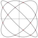
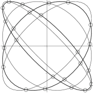
${\displaystyle{{T_{5}(t)-T_{5}(s)}\overwithdelims. .{t-s}}}=0$	${\displaystyle{{T_{7}(t)-T_{7}(s)}\overwithdelims. .{t-s}}}=0$	$\left\{\begin{array}[]{c}{\displaystyle{{T_{7}(t)-T_{7}(s)}\overwithdelims. .{t-s}}}=0\\ {\displaystyle{{T_{5}(t)-T_{5}(s)}\overwithdelims. .{t-s}}}=0\end{array}\right.$

Figure 4: Double point in the parameter space

We thus deduce

Corollary 2.10.

Factorization of $\mathbf{T_{n}(x)-T_{m}(y)}$.
Let $m=ad$, $n=bd$, $(a,b)=1$ and $a$ odd. We have the factorization

$$T_{n}(x)-T_{m}(y)=\mathop{\prod}\limits_{k=0}^{\lfloor{{\textstyle{{d}\overwithdelims. .{2}}}}\rfloor}C_{k}(x,y)$$

where $C_{k}(x,y)=E_{{\textstyle{{2k\pi}\overwithdelims. .{d}}}}(T_{b}(x),T_{a}(y))$.

Proof. We get $T_{n}(x)-T_{m}(y)=T_{d}(T_{b}(x))-T_{d}(T_{a}(y))$ and we conclude using Theorem 2.8. $\Box$

Corollary 2.11.

Let $d=\gcd(n,m)$. The curve $T_{n}(x)=T_{m}(y)$ has $\lfloor{{\textstyle{{d}\overwithdelims. .{2}}}}\rfloor+1$ components, $\lfloor{{\textstyle{{d-1}\overwithdelims. .{2}}}}\rfloor$ of them are Lissajous curves.

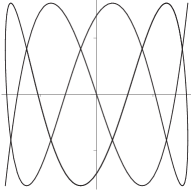
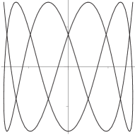
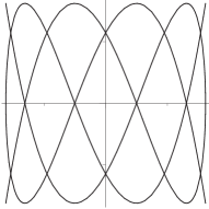
$T_{9}(x)=T_{3}(y)$	$T_{10}(x)=T_{3}(y)$	$T_{10}(x)=T_{4}(y)$

Figure 5: Implicit Chebyshev curves

3 Computing the discriminant polynomial $R_{a,b,c}$

In this section, we will study several methods to compute efficiently a polynomial $R_{a,b,c}\in{\bf Q}[\varphi]$ whose roots are

$${\cal Z}_{a,b,c}=\{\varphi\in{\bf C}|\,\exists(s,t),\,P_{a}(s,t)=P_{b}(s,t)=Q_{c}(s,t,\varphi)=0\}.$$

We will propose a formal computation of $R_{a,b,c}$ using results from Koseleff et al. (2015) on fast operations on Chebyshev forms with a bit complexity in $\widetilde{\mathcal{O}}(n^{4})$ bit operations (with $n=abc$) and also a method using approximate computations (but still providing the exact result) with a bit complexity in $\widetilde{\mathcal{O}}(n^{3})$ operations.

One might use for $R_{a,b,c}$ the generator of the principal ideal $\langle P_{a},P_{b},Q_{c}\rangle\cap{\bf Q}[\varphi]$ which can thus be obtained from any Gröbner basis $\langle P_{a},P_{b},Q_{c}\rangle$ for any monomial order such that $\varphi<s,t$.

Such a straightforward method could be optimized using the structure of the system: $P_{a},P_{b}\in{\bf Q}[s,t]$, $Q_{c}\in{\bf Q}[s,t,\varphi]$ and, moreover, the fact that the leading coefficients of $Q_{c}$ with respect to $\varphi$ belongs to ${\bf Z}$, see Formula (8). Then, one can first compute a Gröbner basis $G_{a,b}$ of $\langle P_{a},P_{b}\rangle$ for any order $<_{a,b}$ and then obtain, without computation, a Gröbner basis $G_{a,b,c}$ of $\langle P_{a},P_{b},Q_{c}\rangle$ for any order compatible with $<_{ab}$ and such that $s,t<\varphi$, by just adding $Q_{c}$ to $G_{a,b}$. Even if the computation time for getting $G_{a,b}$ could be neglected in practice since $a,b<<c$, even if $G_{a,b,c}$ could be easily obtained from $G_{a,b}$, computing $R_{a,b,c}$ still requires to compute the minimal polynomial of $\varphi$ in ${\bf Q}[s,t,\varphi]\bigm{/}\langle P_{a},P_{b},Q_{c}\rangle$ with almost no hope to reach the announced binary complexities.

3.1 The discriminant polynomial $R_{a,b,c}$

As specified in the introduction, the information on multiplicities of the roots of $R_{a,b,c}$ is useless so that the following proposition gives an admissible definition for $R_{a,b,c}$:

Proposition 3.1.

Let $a$, $b$ be coprime integers, $a$ odd, and let $c$ be an integer. Let us consider the polynomial

$$R_{a,b,c}(\varphi)=\mathop{\prod}\limits_{i=1}^{{\textstyle{{a-1}\overwithdelims. .{2}}}}\mathop{\prod}\limits_{j=1}^{b-1}Q_{c}(2\cos({\textstyle{{i\pi}\overwithdelims. .{a}}}+{\textstyle{{j\pi}\overwithdelims. .{b}}}),2\cos({\textstyle{{i\pi}\overwithdelims. .{a}}}-{\textstyle{{j\pi}\overwithdelims. .{b}}}),\varphi).$$

Then $R_{a,b,c}\in{\bf Z}[\varphi]$ and ${\cal C}(a,b,c,\varphi)$ is singular if and only if $R_{a,b,c}=0$.

Proof. The curve ${\cal C}(a,b,c,\varphi)$ is singular if and only if it admits double points. This condition is equivalent to have $t=2\cos({\textstyle{{j\pi}\overwithdelims. .{b}}}+{\textstyle{{i\pi}\overwithdelims. .{a}}})$ and $s=2\cos({\textstyle{{j\pi}\overwithdelims. .{b}}}-{\textstyle{{i\pi}\overwithdelims. .{a}}})$ and $Q_{c}(s,t,\varphi)=0$, for some $1\leq i\leq{\textstyle{{a-1}\overwithdelims. .{2}}}$ and $1\leq j\leq b-1$, from Proposition 2.9. We thus deduce that ${\cal C}(a,b,c,\varphi)$ is singular if and only if $\varphi$ is a root of

$$R_{a,b,c}(\varphi)=\mathop{\prod}\limits_{i=1}^{{\textstyle{{a-1}\overwithdelims. .{2}}}}\mathop{\prod}\limits_{j=1}^{b-1}Q_{c}(2\cos({\textstyle{{i\pi}\overwithdelims. .{a}}}+{\textstyle{{j\pi}\overwithdelims. .{b}}}),2\cos({\textstyle{{i\pi}\overwithdelims. .{a}}}-{\textstyle{{j\pi}\overwithdelims. .{b}}}),\varphi).$$

$Q_{c}(s,t,\varphi)$ is a symmetrical polynomial of ${\bf Z}[\varphi][t,s]$. Let $\alpha_{i}={\textstyle{{i\pi}\overwithdelims. .{a}}}$, $\beta_{j}={\textstyle{{j\pi}\overwithdelims. .{b}}}$ and $s=2\cos(\alpha_{i}+\beta_{j})$, $t=2\cos(\alpha_{i}-\beta_{j})$. From $s+t=4\cos\alpha_{i}\cos\beta_{j}$ and $st=2\cos 2\alpha_{i}+2\cos 2\beta_{j}$, we deduce that $Q_{c}(s,t,\varphi)$ belongs to ${\bf Z}[\varphi,2\cos\alpha_{i}][2\cos\beta_{j}]$.

$$R_{i}=\mathop{\prod}\limits_{j=1}^{b-1}Q_{c}(2\cos(\alpha_{i}+\beta_{j}),\cos(2\alpha_{i}-\beta_{j}),\varphi)$$ (7)

belongs to ${\bf Z}[\varphi,2\cos\alpha_{i}]$ because the roots of $V_{b}\in{\bf Z}[t]$ are the $2\cos\beta_{j}$, $j=1,\ldots,b-1$. From $Q_{c}(-s,-t,-\varphi)=(-1)^{c-1}Q_{c}(s,t,-\varphi)$ we deduce that $\mathop{\prod}\limits_{i=1}^{{a-1}}R_{i}(\varphi)=\pm\mathop{\prod}\limits_{i=1}^{{\textstyle{{a-1}\overwithdelims. .{2}}}}R_{i}(-\varphi)R_{i}(\varphi)\in{\bf Z}[\varphi]$. We thus have $R^{2}_{a,b,c}\in{\bf Z}[\varphi]$ and so it is for $R_{a,b,c}$. $\Box$

Corollary 3.2.

Let $R_{c}(2\cos\alpha,2\cos\beta,\varphi)=Q_{c}(2\cos(\alpha+\beta),\cos(2\alpha-\beta),\varphi)$. Then we have $R^{2}_{a,b,c}=\hbox{\rm Res}_{u}(\hbox{\rm Res}_{v}(R_{c}(u,v,\varphi),V_{a}),V_{b})$.

Proof. In the proof of Proposition 3.1, we have $R_{i}=\hbox{\rm Res}_{v}(R_{c}(2\cos\alpha_{i},v,\varphi),V_{b}(\varphi))$ in Formula (7) and then $\hbox{\rm Res}_{u}(\hbox{\rm Res}_{v}(R_{c}(u,v,\varphi),V_{b}),V_{a})=\mathop{\prod}\limits_{i=1}^{a-1}R_{i}(\varphi)=R_{a,b,c}^{2}.$ $\Box$

Example. When $a=3$, $b=4$, $c=5$, we find that

$$R_{a,b,c}=\left(5{\varphi}^{4}+15{\varphi}^{2}-1\right)\cdot\left(25{\varphi}^{8}-50{\varphi}^{6}+35{\varphi}^{4}-20{\varphi}^{2}+1\right).$$

There are exactly 6 critical values that are symmetrical about the origin.

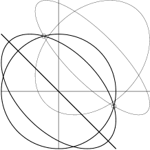
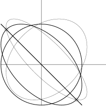
$\varphi=.590$		$\varphi=.128$		$\varphi=.117$

Figure 6: $P_{3}=0,P_{4}=0,Q_{5}=0$

For these values of $\varphi$, the curve $Q_{5}(s,t,\varphi)=0$, which is translated from the curve $P_{5}(s,t)=0$ by the vector $(\varphi,\varphi)$, meets the points $\{P_{3}=0,P_{4}=0\}$ (see Figure 6).

3.2 Factorizing $R_{a,b,c}$ into low-degree polynomials

Formula (6) will give us an explicit formula for the polynomial $R_{a,b,c}$ as a product of polynomials of degree 1 or 2 with coefficients in ${\bf Z}[2\cos{\textstyle{{\pi}\overwithdelims. .{a}}},2\cos{\textstyle{{\pi}\overwithdelims. .{b}}},2\cos{\textstyle{{\pi}\overwithdelims. .{c}}}]$. The interest of having such an expression is to make possible the use of efficient tools for evaluating trigonometric expressions, such as those proposed in (Koseleff et al., 2015).

Let us introduce the following polynomials:

Definition 3.3.

We set $P_{\alpha,\beta,{\textstyle{{\pi}\overwithdelims. .{2}}}}(\varphi)=\varphi+2\cos\alpha\cos\beta$ and

$$P_{\alpha,\beta,\gamma}(\varphi)=\varphi^{2}+4\varphi\cos\alpha\cos\beta+4{\displaystyle{{(\cos^{2}\alpha-\cos^{2}\gamma)(\cos^{2}\beta-\cos^{2}\gamma)}\overwithdelims. .{\sin^{2}\gamma}}},$$

for $\gamma\not={\textstyle{{\pi}\overwithdelims. .{2}}}$.

When $\gamma\not={\textstyle{{\pi}\overwithdelims. .{2}}}$, we have $4\sin^{2}\gamma P_{\alpha,\beta,\gamma}=E_{2\gamma}(2\cos(\alpha+\beta)+\varphi,2\cos(\alpha-\beta)+\varphi)$. When $\gamma={\textstyle{{\pi}\overwithdelims. .{2}}}$, we have $2\sin\gamma P_{\alpha,\beta,\gamma}=E_{\pi}$. Then, using Equation (6) and $\mathop{\prod}\limits_{k=1}^{c-1}2\sin{\textstyle{{k\pi}\overwithdelims. .{c}}}=c$, we deduce that

$$Q_{c}(2\cos(\alpha+\beta),2\cos(\alpha-\beta),\varphi)=c\mathop{\prod}\limits_{k=1}^{\lfloor{{\textstyle{{c}\overwithdelims. .{2}}}}\rfloor}P_{\alpha,\beta,{\textstyle{{k\pi}\overwithdelims. .{c}}}}(\varphi),$$ (8)

and we get the factorization of the polynomial $R_{a,b,c}$:

Proposition 3.4.

Let $a,b$ be nonnegative coprime integers, $a$ odd, and $c$ be an integer. Then

$$R_{a,b,c}(\varphi)=c^{(a-1)(b-1)/2}\mathop{\prod}\limits_{i=1}^{{\textstyle{{a-1}\overwithdelims. .{2}}}}\mathop{\prod}\limits_{j=1}^{b-1}\mathop{\prod}\limits_{k=1}^{\lfloor{{\textstyle{{c}\overwithdelims. .{2}}}}\rfloor}P_{{\textstyle{{i\pi}\overwithdelims. .{a}}},{\textstyle{{j\pi}\overwithdelims. .{b}}},{\textstyle{{k\pi}\overwithdelims. .{c}}}}(\varphi).$$ (9)

We have written $R_{a,b,c}$ as the product of second or first-degree polynomials $P_{\alpha,\beta,\gamma}$ in ${\bf Z}[2\cos{\textstyle{{\pi}\overwithdelims. .{a}}},2\cos{\textstyle{{\pi}\overwithdelims. .{b}}},2\cos{\textstyle{{\pi}\overwithdelims. .{c}}}][\varphi]$.

Remark 3.5.

There are two cases to consider in Formula (9). If $c$ is odd then $R_{a,b,c}$ appears as the product

$$R^{(1)}_{a,b,c}(\varphi)=\mathop{\prod}\limits_{i=1}^{{\textstyle{{a-1}\overwithdelims. .{2}}}}\mathop{\prod}\limits_{j=1}^{b-1}\mathop{\prod}\limits_{k=1}^{{\textstyle{{c-1}\overwithdelims. .{2}}}}4\sin^{2}{\textstyle{{k\pi}\overwithdelims. .{c}}}P_{{\textstyle{{i\pi}\overwithdelims. .{a}}},{\textstyle{{j\pi}\overwithdelims. .{b}}},{\textstyle{{k\pi}\overwithdelims. .{c}}}}(\varphi).$$ (10)

If $c$ is even we have to multiply the previous product by

$$R^{(0)}_{a,b,c}(\varphi)=\mathop{\prod}\limits_{i=1}^{{\textstyle{{a-1}\overwithdelims. .{2}}}}\mathop{\prod}\limits_{j=1}^{b-1}(2\varphi+4\cos\alpha\cos\beta).$$ (11)

3.3 Computing $R_{a,b,c}$ using Chebyshev polynomials

In this section, we will use the algorithms for evaluating and using trigonometric expressions in the form $F=\sum_{k=0}^{d}f_{k}\cos k{\textstyle{{\pi}\overwithdelims. .{n}}}$, $f_{k}\in{\bf Z}$, that are developed in (Koseleff et al., 2015).

The Chebyshev basis $(1,T_{i},i\geq 1)$ is particularly adapted for our computations. We say that $f=f_{0}+\sum_{i=1}^{d}f_{i}T_{i}$, $f_{i}\in{\bf Z}$, is a Chebyshev form.

Definition 3.6.

Let $f=f_{0}+\sum_{i=1}^{d}f_{i}T_{i}$ be a Chebyshev form. We denote by $\tau(f)$ the maximum bitsize of its coefficients. We denote by $||f||_{T}$ the norm $\left|f_{0}\right|+2\sum_{i=1}^{d}\left|f_{i}\right|$.

The cyclotomic extension ${\bf Q}[2\cos{\textstyle{{\pi}\overwithdelims. .{n}}}]$ is ${\bf Q}[x]/(M_{n})$ where $M_{n}$ is the minimal polynomial in ${\bf Z}[x]$ of $2\cos{\textstyle{{\pi}\overwithdelims. .{n}}}$. In (Koseleff et al., 2015), it is shown that $M_{n}$ is monic of degree ${\textstyle{{1}\overwithdelims. .{2}}}\varphi(2n)$, where $\varphi:{\bf N}^{*}\to{\bf N}$ is the Euler totient function. $M_{n}$ can be computed in the Chebyshev basis in $\widetilde{\mathcal{O}}(n)$ arithmetic operations or $\widetilde{\mathcal{O}}(n^{2})$ bit operations and $\tau(M_{n})=\mathcal{O}(n)$, see (Koseleff et al., 2015, Prop. 16).

Lemma 3.7.

(Koseleff et al., 2015) Let $f=f_{0}+\sum_{i=1}^{n-1}f_{i}T_{i}$ and $g=g_{0}+\sum_{i=1}^{n-1}g_{i}T_{i}$ be Chebyshev forms with $\tau(f),\tau(g)\leq\tau$. Then one can compute $h=h_{0}+\sum_{i=1}^{n-1}h_{i}T_{i}$ where $h\equiv f\cdot g\,(\hbox{\rm mod}\,M_{n})$ in $\widetilde{\mathcal{O}}(n\tau)$ bit operations and $\tau(h)\leq\tau(f)+\tau(g)+\log_{2}n+1$.

We thus deduce

Corollary 3.8.

Let $P=\sum_{i=0}^{D}p_{i}(2\cos{\textstyle{{\pi}\overwithdelims. .{n}}})\varphi^{i}$ and $Q=\sum_{i=0}^{d}q_{i}(2\cos{\textstyle{{\pi}\overwithdelims. .{n}}})\varphi^{i}$ be two polynomials in ${\bf Z}[2\cos{\textstyle{{\pi}\overwithdelims. .{n}}}][\varphi]$. Suppose that the Chebyshev forms $p_{i}=\sum_{j=0}^{n-1}p_{i,j}T_{j}$ and $q_{i}=\sum_{j=0}^{n-1}q_{i,j}T_{j}$ satisfy $\tau(p_{i})\leq\tau$ and $\tau(q_{i})\leq\tau^{\prime}\leq\tau$.

Then we have $P\cdot Q=\sum_{i=0}^{D+d}h_{i}(2\cos{\textstyle{{\pi}\overwithdelims. .{n}}})\varphi^{i}$ where $h_{i}=\sum_{j=0}^{n-1}h_{i,j}T_{j}$ satisfy $\tau(h_{i})\leq\tau+\tau^{\prime}+\log_{2}n+\log_{2}d$. One can compute all the Chebyshev forms $[{\cal T}]h_{i}$ in $\mathcal{O}(dD)$ operations in ${\bf Z}[2\cos{\textstyle{{\pi}\overwithdelims. .{n}}}]$ that is $\widetilde{\mathcal{O}}(dDn\tau)$ binary operations.

Proof. We get $P\cdot Q=\sum_{i=0}^{d+D}h_{i}\varphi^{i}$ where $h_{i}=\sum_{j=0}^{d}p_{i-j}q_{j}$. Each $p_{i-j}q_{j}$ may be computed in $\widetilde{\mathcal{O}}(n\tau)$ binary operations and therefore all the coefficients $h_{i}$ may be computed in $\widetilde{\mathcal{O}}(d(d+D)n\tau)$ binary operations, using Lemma 3.7. Furthermore $\tau(h_{i})\leq\tau+\tau^{\prime}+\log_{2}n+\log d$, using Lemma 3.7. $\Box$

We deduce

Corollary 3.9.

Let $P_{i}=\sum_{j=0}^{d}p_{i,j}(2\cos{\textstyle{{\pi}\overwithdelims. .{n}}})\varphi^{j}$ be polynomials in ${\bf Z}[2\cos{\textstyle{{\pi}\overwithdelims. .{n}}}][\varphi]$ with $\tau(p_{i,j})\leq\tau$. Then we have $P=\mathop{\prod}\limits_{i=1}^{k}P_{i}=\sum_{i=0}^{dk}h_{i}(2\cos{\textstyle{{\pi}\overwithdelims. .{n}}})\varphi^{j}$ where $h_{i}=\sum_{j=0}^{n-1}h_{i,j}T_{j}$ satisfy $\tau(h_{i})\leq k\tau+k\log_{2}nd$. One can compute $P$ in $\widetilde{\mathcal{O}}(d^{2}k^{3}n\tau)$ binary operations.

Proof. Let $Q_{i}=P_{1}\cdots P_{i}$. Then we have, from Corollary 3.8, $\tau(Q_{i+1})\leq\tau(Q_{i})+\tau+\log_{2}nd\leq(i+1)(\tau+\log_{2}nd)$. One computes $Q_{i+1}$ from $Q_{i}$ in $\widetilde{\mathcal{O}}(\tau(Q_{i})d(id+d)n\tau)=\widetilde{\mathcal{O}}(i^{2}d^{2}n\tau)$ binary operations, using Corollary 3.8. At the end we get $Q_{k}$ in $\widetilde{\mathcal{O}}(k^{3}d^{2}n\tau)$ binary operations. $\Box$

We then compute $R_{a,b,c}$ in ${\bf Z}[2\cos{\textstyle{{\pi}\overwithdelims. .{a}}},2\cos{\textstyle{{\pi}\overwithdelims. .{b}}},2\cos{\textstyle{{\pi}\overwithdelims. .{c}}}][\varphi]\subset{\bf Z}[2\cos{\textstyle{{\pi}\overwithdelims. .{n}}}][\varphi]$, using Formulas (10) and (9) and Corollary 3.9.

Proposition 3.10.

Let $a$ and $b$ be coprime integers, $a$ odd, and $c$ an integer. One can compute $R_{a,b,c}$ as an element of ${\bf Z}[2\cos{\textstyle{{\pi}\overwithdelims. .{n}}}][\varphi]$ in $\mathcal{O}(n^{4})$ binary operations.

Proof. We want to compute the product of the polynomials $4\sin^{2}{\textstyle{{k\pi}\overwithdelims. .{c}}}\cdot P_{{\textstyle{{i\pi}\overwithdelims. .{a}}},{\textstyle{{j\pi}\overwithdelims. .{b}}},{\textstyle{{k\pi}\overwithdelims. .{c}}}}(\varphi)$ in Formula (10). We write, for $k{\textstyle{{\pi}\overwithdelims. .{c}}}\not={\textstyle{{\pi}\overwithdelims. .{2}}}$:

$$4\sin^{2}{\textstyle{{k\pi}\overwithdelims. .{c}}}\cdot P_{{\textstyle{{i\pi}\overwithdelims. .{a}}},{\textstyle{{j\pi}\overwithdelims. .{b}}},{\textstyle{{k\pi}\overwithdelims. .{c}}}}(\varphi)={\displaystyle{{1}\overwithdelims. .{4}}}\Bigl{(}f_{2}(2\cos{\textstyle{{\pi}\overwithdelims. .{n}}})\varphi^{2}+f_{1}(2\cos{\textstyle{{\pi}\overwithdelims. .{n}}})\varphi+f_{0}(2\cos{\textstyle{{\pi}\overwithdelims. .{n}}})\Bigr{)}$$

where

$$\begin{array}[]{rcl}f_{2}&=&2-T_{{2\,kab}},\\ f_{1}&=&2\,T_{{cja-cib}}+2\,T_{{cja+cib}}-T_{{2\,kab+cja-cib}}-T_{{2\,kab-cja+cib}}-\\ &&\quad T_{{2\,kab-cja-cib}}-T_{{2\,kab+cja+cib}},\\ f_{0}&=&2+T_{{2\,cja-2\,cib}}+T_{{2\,cja+2\,cib}}+T_{{4\,kab}}\\ &&\quad-T_{{2\,kab-2\,cib}}-T_{{2\,kab+2\,cib}}-T_{{2\,kab-2\,cja}}-T_{{2\,kab+2\,cja}}.\end{array}$$ (12)

If $c$ is even, we also have to compute the product of $2\varphi+4\cos\alpha\cos\beta$ in Formula (11). We write

$$2\varphi+4\cos\alpha\cos\beta={\displaystyle{{1}\overwithdelims. .{2}}}\Bigl{(}g_{1}(2\cos{\textstyle{{\pi}\overwithdelims. .{n}}})\varphi+g_{0}(2\cos{\textstyle{{\pi}\overwithdelims. .{n}}})\Bigr{)}$$

where

$$g_{1}=2,\quad g_{0}=T_{{cja-cib}}+T_{{cja+cib}}.$$ (13)

Using $T_{n+i}\equiv T_{n-i}\equiv-T_{i}\,(\hbox{\rm mod}\,M_{n})$, we can write $f_{0}$, $f_{1}$ and $f_{2}$ as Chebyshev forms of degree at most $n-1$ and $\tau(f_{i})\leq 4$. We also have $\tau(g_{i})\leq 2$.

Using Corollary 3.9, with $k=N={\textstyle{{1}\overwithdelims. .{2}}}(a-1)(b-1)(c-1)$ and $\tau=4$, we see that we can compute the product $2^{2N}R_{a,b,c}\in{\bf Z}[2\cos{\textstyle{{\pi}\overwithdelims. .{n}}}][\varphi]$ in $\widetilde{\mathcal{O}}(n^{4})$ binary operations. Each coefficient of $2^{2N}R_{a,b,c}$ has size $\tau$ bounded by $\widetilde{\mathcal{O}}(n)$, using Corollary 3.9. $\Box$

3.4 Computing $R_{a,b,c}$ by using numerical approximations

One might use the expression of $R_{a,b,c}$ in ${\bf Z}[2\cos{\textstyle{{\pi}\overwithdelims. .{n}}}][\varphi]$ and approximate the coefficients of $2^{N}R_{a,b,c}$ with accuracy less than ${\textstyle{{1}\overwithdelims. .{2}}}$ in order to get $R_{a,b,c}$ as an element of ${\bf Z}[\varphi]$: using Corollary 3.12 below, it would take $\widetilde{\mathcal{O}}(n^{2})$ binary operations for each coefficient and thus $\widetilde{\mathcal{O}}(n^{3})$ binary operations to get the entire polynomial.

We will improve this strategy by using numerical approximations of the factors $4\sin^{2}\gamma\cdot P_{\alpha,\beta,\gamma}$ in ${\bf Q}[\varphi]$. We shall use the following technical lemma (Koseleff et al., 2015, Lemma 18) several times:

Lemma 3.11.

(Brent, 1975, 1976) Let $0\leq k\leq n$ and $\gamma=2\cos k{\textstyle{{\pi}\overwithdelims. .{n}}}$. Let $\ell\in{\bf Z}_{>0}$. One can compute $c\in{\bf Q}$, of bitsize $\tau(c)\leq\ell$ such that $\left|c-\gamma\right|\leq 2^{-\ell}$ in $\widetilde{\mathcal{O}}(\ell+\log n)$ bit operations.

From this Lemma, we deduce

Corollary 3.12.

(Koseleff et al., 2015, Cor. 19) Let $0\leq k\leq n$ and $\gamma=2\cos k{\textstyle{{\pi}\overwithdelims. .{n}}}$. Let $\ell\in{\bf Z}_{>0}$. Let $f$ be the Chebyshev form $f_{0}+\sum_{i=1}^{n-1}f_{i}T_{i}$ with $\tau(f)\leq\tau$. One computes $\widetilde{F}\in{\bf Q}$ of bitsize $\widetilde{\mathcal{O}}(n\tau+\ell)$ such that $\left|\widetilde{F}-f(\gamma)\right|\leq 2^{-\ell}$ in $\widetilde{\mathcal{O}}(n\ell+n\tau)$ bit operations.

One computes $F^{-}$ and $F^{+}$ of bitsize $\widetilde{\mathcal{O}}(n\tau+\ell)$ such that $F^{-}\leq F\leq F^{+}$ and $F^{+}-F^{-}\leq 2^{-\ell}$ in $\widetilde{\mathcal{O}}(n\ell+n\tau)$ bit operations.

We first show

Lemma 3.13.

Let $P_{i}=a_{i}\varphi^{2}+b_{i}\varphi+c_{i}$, $i=1,\ldots,N$, be polynomials in ${\bf R}_{\leq 2}[\varphi]$. Let $\hat{P}_{i}\in{\bf R}_{\leq 2}[\varphi]$, such that

$$||P_{i}||_{\infty}\leq M,\quad||\hat{P}_{i}-P_{i}||_{\infty}\leq\delta.$$

Then we have

$$||\mathop{\prod}\limits_{i=1}^{N}P_{i}-\mathop{\prod}\limits_{i=1}^{N}\hat{P}_{i}||_{\infty}\leq\delta\,N\,3^{N}(M+\delta)^{N}.$$

Proof. It is straightforward that if $\deg Q\leq 2$ then $||PQ||_{\infty}\leq 3||P||_{\infty}||Q||_{\infty}$. We thus deduce by induction, with $||\hat{P}_{i}||_{\infty}\leq M+\delta$, that $||P_{1}\cdots P_{k}||_{\infty}\leq 3^{k-1}M^{k}$ and $||\hat{P}_{1}\cdots\hat{P}_{k}||_{\infty}\leq 3^{k-1}(M+\delta)^{k}$.

Suppose that $||P_{1}\cdots P_{k}-\hat{P}_{1}\cdots\hat{P}_{k}||_{\infty}\leq\delta_{k}$, then we obtain

$||P_{1}\cdots P_{k+1}-\hat{P}_{1}\cdots\hat{P}_{k+1}||_{\infty}$

$\begin{array}[]{rcl}&=&||P_{1}\cdots P_{k}(P_{k+1}-\hat{P}_{k+1})+(P_{1}\cdots P_{k}-\hat{P}_{1}\cdots\hat{P}_{k})\hat{P}_{k+1}||_{\infty}\\ &\leq&||P_{1}\cdots P_{k}(P_{k+1}-\hat{P}_{k+1})||_{\infty}+||(P_{1}\cdots P_{k}-\hat{P}_{1}\cdots\hat{P}_{k})\hat{P}_{k+1}||_{\infty}\\ &=&3^{k}M^{k}\delta+3\delta_{k}(M+\delta)\end{array}$.

We deduce that $\delta_{k+1}\leq 3(M+\delta)\delta_{k}+(3M)^{k}\delta.$ Let $u_{k}={\displaystyle{{\delta_{k}}\overwithdelims. .{3^{k}(M+\delta)^{k}}}}$, we deduce that

$$u_{k+1}-u_{k}\leq{\displaystyle{{\delta}\overwithdelims. .{3(M+\delta)}}}\Bigl{(}{\displaystyle{{M}\overwithdelims. .{M+\delta}}}\Bigr{)}^{k}\leq\delta.$$

We thus obtain that $u_{k+1}\leq u_{1}+k\delta=(k+1)\delta$. $\Box$

Lemma 3.14.

Let $P_{i}=a_{i}\varphi^{2}+b_{i}\varphi+c_{i}$, $i=1,\ldots,N$, be polynomials in ${\bf Q}_{\leq 2}[\varphi]$ with all coefficients being dyadic numbers such that $\tau(P_{i})\leq\tau$. Then $P=\mathop{\prod}\limits_{i=1}^{N}P_{i}$ may be computed in $\widetilde{\mathcal{O}}(N^{2}\tau)$ binary operations and we have $\tau(P)\leq N\tau+(N-1)\log_{2}3$.

Proof. From $||UP_{i}||_{\infty}\leq 3||U||_{\infty}||P_{i}||_{\infty}$, we obtain that $||P||_{\infty}\leq 3^{N-1}2^{N\tau}$. Let $m=\lceil\log_{2}N\rceil$. We get $P_{i}=1$ for $N<i\leq 2^{m}$ and we compute by induction $P=\mathop{\prod}\limits_{i=1}^{2^{m}-1}P_{i}\cdot\mathop{\prod}\limits_{i=1}^{2^{m}-1}P_{2^{m-1}+i}$, using fast multiplication in ${\bf Q}[\varphi]$.

Let us suppose that we have computed $Q_{0}=\mathop{\prod}\limits_{i=1}^{2^{m}-1}P_{i}$ and $Q_{1}=\mathop{\prod}\limits_{i=1}^{2^{m}-1}P_{2^{m-1}+i}$ in $\widetilde{\mathcal{O}}(2^{2m-2}\tau)$ binary operations. $\tau(Q_{1}),\tau(Q_{2})\leq 2^{m-1}(\tau+\log_{2}3)$ and we obtain $Q_{1}\cdot Q_{2}$ in $\widetilde{\mathcal{O}}(2^{2m}\tau)$ binary operations. At the end, we have computed $P$ in $\sum_{i=1}^{m}\widetilde{\mathcal{O}}(2^{2i}\tau)=\widetilde{\mathcal{O}}(N^{2}\tau)$ binary operations. $\Box$

Applying the above results to the computation of $R_{a,b,c}$, we get:

Proposition 3.15.

Let $a$ and $b$ be coprime integers, $a$ odd, and $c$ an integer. One can compute $R_{a,b,c}$ in $\widetilde{\mathcal{O}}(n^{3})$ binary operations.

Proof. Let $N={\textstyle{{1}\overwithdelims. .{2}}}(a-1)(b-1)\lfloor{{\textstyle{{c}\overwithdelims. .{2}}}}\rfloor$. We have $||4\sin^{2}\gamma P_{\alpha,\beta,\gamma}||_{\infty}\leq 16-{\textstyle{{4}\overwithdelims. .{c^{2}}}}=M$. We compute each coefficient of $4\sin^{2}\gamma P_{\alpha,\beta,\gamma}$ with accuracy $\delta=2^{-6N+1}$. We obtain $N$ polynomials ${\hat{P}_{\alpha,\beta,\gamma}}$ whose coefficients are dyadic numbers of size bounded by $\tau=6N+1$ and whose norm is bounded by $M+\delta\leq 16$.

We then compute $\mathop{\prod}\limits{\hat{P}_{\alpha,\beta,\gamma}}$ in ${\bf Q}[\varphi]$ in $\widetilde{\mathcal{O}}(N^{3})$ binary operations, using Lemma 3.14 with $\tau=6N+1$.

We have $||R_{a,b,c}-\mathop{\prod}\limits{\hat{P}_{\alpha,\beta,\gamma}}||\leq 2^{-6N+1}N3^{N}\cdot 16^{N}\leq{\displaystyle{{1}\overwithdelims. .{2}}}$, using Lemma 3.13. $\Box$

4 Computing the real roots of $R_{a,b,c}$

In this section, the goal is to isolate efficiently the real roots of $R_{a,b,c}$. As seen previously, the polynomial $R_{a,b,c}$ can be computed in $\widetilde{\mathcal{O}}(n^{3})$ binary operations. Our first lemma gives estimates for the size of the coefficients of $P_{\alpha,\beta,\gamma}$ such that $||R_{a,b,c}||_{1}\leq 6^{N}$ and thus, running recent algorithms such as in (Mehlhorn and Sagraloff, 2016), the (real) roots of $R_{a,b,c}$ can be isolated in $\widetilde{\mathcal{O}}(n^{3})$ binary operations.

In the next subsections, we will show that, in fact, the computation of the real roots of $R_{a,b,c}$ can be done in $\widetilde{\mathcal{O}}(n^{2})$ bit operations. This result is due to many properties of the roots of $R_{a,b,c}$, in particular the minimum distance between two distinct real roots that is greater than $2^{-8n}$ (while the worst case for a polynomial of degree $n$ with coefficients of bitsize in $\widetilde{\mathcal{O}}(n)$ is in $\widetilde{\mathcal{O}}(n^{2})$) and roots bounded in module by $4$ (while the theoretical bound would have been in $\widetilde{\mathcal{O}}(n)$).

Note that these two properties on the real roots could certainly be used to adapt the complexity of the algorithm from Mehlhorn and Sagraloff (2016) or even the one from Rouillier and Zimmermann (2003), which has been used in (Koseleff et al., 2010), but we will propose a dedicated algorithm for isolating the roots of $R_{a,b,c}$.

Let us start with the estimates for the size of the coefficients of $P_{\alpha,\beta,\gamma}$ and $||R_{a,b,c}||$:

Lemma 4.1 (Estimates).

Let $a$ and $b$ coprime integers, $a$ odd, and $c$ an integer. Let $N={\textstyle{{1}\overwithdelims. .{2}}}(a-1)(b-1)(c-1)$ and $R_{a,b,c}(\varphi)=\sum_{i=0}^{N}a_{i}\varphi^{i}$. The we have $||R_{a,b,c}||_{1}=\sum_{i=1}^{N}\left|a_{i}\right|\leq 6^{N}$.

Proof. According to 3.5, there are two cases to consider in Formula (9). If $c$ is odd then $R_{a,b,c}$ appears as the product

$$R^{(1)}_{a,b,c}=\mathop{\prod}\limits_{i=1}^{{\textstyle{{a-1}\overwithdelims. .{2}}}}\mathop{\prod}\limits_{j=1}^{b-1}\mathop{\prod}\limits_{k=1}^{{\textstyle{{c-1}\overwithdelims. .{2}}}}4\sin^{2}{\textstyle{{k\pi}\overwithdelims. .{c}}}P_{{\textstyle{{i\pi}\overwithdelims. .{a}}},{\textstyle{{j\pi}\overwithdelims. .{b}}},{\textstyle{{k\pi}\overwithdelims. .{c}}}}(\varphi).$$ (14)

If $c$ is even we have to multiply the previous product by

$$R^{(0)}_{a,b,c}=\mathop{\prod}\limits_{i=1}^{{\textstyle{{a-1}\overwithdelims. .{2}}}}\mathop{\prod}\limits_{j=1}^{b-1}(2\varphi+4\cos\alpha\cos\beta).$$ (15)

Let $P=\sum_{i=0}^{m}a_{i}\varphi^{i}\in{\bf R}[\varphi]$ and $Q=\sum_{i=0}^{m}b_{i}\varphi^{i}\in{\bf R}[\varphi]$. We say that $P\prec Q$ if $\left|a_{i}\right|\leq b_{i}$, $i=0,\ldots,m$. It is straightforward that if $P\prec Q$ then $||P||_{1}\leq||Q||_{1}$ and that if $P_{1}\prec Q_{1}$ and $P_{2}\prec Q_{2}$ then $||P_{1}P_{2}||_{1}\leq||Q_{1}Q_{2}||_{1}$.

We have $\varphi+2\cos{\textstyle{{i\pi}\overwithdelims. .{a}}}\cos{\textstyle{{j\pi}\overwithdelims. .{b}}}\prec\varphi+2$, and we deduce that $R^{(0)}_{a,b,c}\prec(2\varphi+4)^{(a-1)(b-1)/2}$.

If $\gamma={\textstyle{{k\pi}\overwithdelims. .{2}}}\not={\textstyle{{\pi}\overwithdelims. .{2}}}$ then

$$\sin^{2}\gamma P_{\alpha,\beta,\gamma} = \sin^{2}\gamma\,\cdot\varphi^{2}+4\varphi\cdot\cos\alpha\cos\beta\sin^{2}\gamma$$

$$\quad\quad\quad+4(\cos^{2}\alpha-\cos^{2}\gamma)(\cos^{2}\beta-\cos^{2}\gamma)$$

$$\prec (\varphi+2)^{2}.$$

We then deduce that $R^{(1)}_{a,b,c}\prec\Bigl{(}(2\varphi+4)^{2\lfloor{{\textstyle{{c-1}\overwithdelims. .{2}}}}\rfloor}\Bigr{)}^{(a-1)(b-1)/2}$ and $R_{a,b,c}\prec(2\varphi+4)^{N}$, that is $||R_{a,b,c}||_{1}\leq 2^{N}||(\varphi+2)^{N}||_{1}=6^{N}$. $\Box$

4.1 Factor’s roots

Let $\alpha={\textstyle{{i\pi}\overwithdelims. .{a}}}$, $\beta={\textstyle{{j\pi}\overwithdelims. .{b}}}$ and $\gamma={\textstyle{{k\pi}\overwithdelims. .{c}}}$ with $1\leq i\leq{\textstyle{{a-1}\overwithdelims. .{2}}},\ 1\leq j\leq b-1,\ 1\leq k\leq\lfloor{{\textstyle{{c-1}\overwithdelims. .{2}}}}\rfloor$.

If $\gamma={\textstyle{{\pi}\overwithdelims. .{2}}}$, the unique root of $P_{\alpha,\beta,{\textstyle{{\pi}\overwithdelims. .{2}}}}$ is $-2\cos\alpha\cos\beta$. If $\gamma\not={\textstyle{{\pi}\overwithdelims. .{2}}}$, the discriminant of $P_{\alpha,\beta,\gamma}$ is

$$\Delta_{\alpha,\beta,\gamma}=16\cos^{2}\gamma\Bigl{(}1-{\displaystyle{{\sin^{2}\alpha\sin^{2}\beta}\overwithdelims. .{\sin^{2}\gamma}}}\Bigr{)}.$$ (16)

It has the same sign as

$$\sin\gamma-\sin\alpha\sin\beta,$$ (17)

because $\sin\alpha,\sin\beta$ and $\sin\gamma$ are nonnegative. The equation $\Delta_{\alpha,\beta,\gamma}=0$ is related to the equation

$$\sin r_{1}\pi\sin r_{2}\pi=\sin r_{3}\pi\sin r_{4}\pi,\quad r_{1},r_{2},r_{3},r_{4}\in{\bf Q}.$$ (18)

All the solutions of Equation (18) are known:

Lemma 4.2.

(Myerson, 1993; Conway and Jones, 1976) Equation (18) admits the one-parameter infinite family of solutions corresponding to

$$\sin{\textstyle{{\pi}\overwithdelims. .{6}}}\sin\theta=\sin{\textstyle{{\theta}\overwithdelims. .{2}}}\sin({\textstyle{{\pi}\overwithdelims. .{2}}}-{\textstyle{{\theta}\overwithdelims. .{2}}}),$$

and a finite number of solutions listed in (Myerson, 1993), for which the denominators of the $r_{i}$ are not coprime.

We thus deduce

Proposition 4.3.

Let $\alpha={\textstyle{{i\pi}\overwithdelims. .{a}}}$, $\beta={\textstyle{{j\pi}\overwithdelims. .{b}}}$ and $\gamma={\textstyle{{k\pi}\overwithdelims. .{c}}}$, where $(a,b)=1$ and $a$ is odd. $P_{\alpha,\beta,\gamma}$ has a double root if and only if $\beta={\textstyle{{\pi}\overwithdelims. .{2}}}$ and $\gamma=\alpha$. In this case, the double root is $\varphi=0$.

Proof. $P_{\alpha,\beta,\gamma}$ has a double root if and only if $\mathrm{Disc}\,(P_{\alpha,\beta,\gamma})=0$, that is to say $\sin\gamma\cdot 1=\sin\alpha\sin\beta$. We conclude with the help of Lemma 4.2. $\Box$

The knowledge of the sign of (17) then gives explicit formulas for the real roots of $P_{\alpha,\beta,\gamma}$ that we will explain in the next section. But we also have to decide if the roots are distinct or what are their multiplicities.

4.2 Multiple roots

It may happen that $R_{a,b,c}$ has multiple real roots. Two cases may occur: $P_{\alpha,\beta,\gamma}$ has a double root (that is $\mathrm{Disc}\,(P_{\alpha,\beta,\gamma})=0$) or $P_{\alpha_{1},\beta_{1},\gamma_{1}}$ and $P_{\alpha_{2},\beta_{2},\gamma_{2}}$ have a common root (that is $\hbox{\rm Res}_{\varphi}(P_{\alpha_{1},\beta_{1},\gamma_{1}},P_{\alpha_{2},\beta_{2},\gamma_{2}})=0$).

In the particular case when $\alpha_{1}=\alpha_{2}$ and $\beta_{1}=\beta_{2}$, or $\gamma_{1}=\gamma_{2}={\textstyle{{\pi}\overwithdelims. .{2}}}$, the equation $\hbox{\rm Res}_{\varphi}(P_{\alpha_{1},\beta_{1},\gamma_{1}},P_{\alpha_{2},\beta_{2},\gamma_{2}})=0$ may be solved using Lemma 4.2.

Proposition 4.4.

Let $\alpha_{1}={\textstyle{{i_{1}\pi}\overwithdelims. .{a}}}$, $\beta_{1}={\textstyle{{j_{1}\pi}\overwithdelims. .{b}}}$, and $\alpha_{2}={\textstyle{{i_{2}\pi}\overwithdelims. .{a}}}$, $\beta_{2}={\textstyle{{j_{2}\pi}\overwithdelims. .{b}}}$, where $(a,b)=1$. $P_{\alpha_{1},\beta_{1},{\textstyle{{\pi}\overwithdelims. .{2}}}}$ and $P_{\alpha_{2},\beta_{2},{\textstyle{{\pi}\overwithdelims. .{2}}}}$ have a common root if and only if $\alpha_{1}=\alpha_{2}$ and $\beta_{1}=\beta_{2}$.

Proof. The equation $\cos\alpha_{1}\cos\beta_{1}=\cos\alpha_{2}\cos\beta_{2}$ admits the unique solution $\alpha_{1}=\alpha_{2}$ and $\beta_{1}=\beta_{2}$, using Lemma 4.2. $\Box$

Proposition 4.5.

Let $\alpha={\textstyle{{i\pi}\overwithdelims. .{a}}}$, $\beta={\textstyle{{j\pi}\overwithdelims. .{b}}}$ and $\gamma_{1}={\textstyle{{k_{1}\pi}\overwithdelims. .{c}}}$, $\gamma_{2}={\textstyle{{k_{2}\pi}\overwithdelims. .{c}}}$, where $(a,b)=1$, $a$ is odd and $\gamma_{1}\not=\gamma_{2}$. Then $P_{\alpha,\beta,\gamma_{1}}$ and $P_{\alpha,\beta,\gamma_{2}}$ have a common root $\varphi$ if and only if they are equal and one of the following cases occurs:

1. $\sin\alpha=\sin\gamma_{1}$, $\sin\beta=\sin\gamma_{2}$. Their common roots are $\varphi=0$ and $\varphi=-4\cos\alpha\cos\beta$.

2. $\beta={\textstyle{{\pi}\overwithdelims. .{6}}}$, $\gamma_{1}={\textstyle{{1}\overwithdelims. .{2}}}\alpha$, $\gamma_{2}={\textstyle{{\pi}\overwithdelims. .{2}}}-\alpha$. In this case their common roots are $\varphi=-2\cos(\alpha\pm{\textstyle{{\pi}\overwithdelims. .{6}}})$.

Proof. In this case $\hbox{\rm Res}(P_{\alpha,\beta,\gamma_{1}},P_{\alpha,\beta,\gamma_{2}})=0$, that is to say

$$(\sin^{2}\gamma_{1}-\sin^{2}\gamma_{2})(\sin^{2}\gamma_{1}\sin^{2}\gamma_{2}-\sin^{2}\alpha\sin^{2}\beta)=0$$ (19)

We conclude using Lemma 4.2. $\Box$

In case when $\alpha_{1}\not=\alpha_{2}$ or $\beta_{1}\not=\beta_{2}$, $\hbox{\rm Res}_{\varphi}(P_{\alpha_{1},\beta_{1},\gamma_{1}},P_{\alpha_{2},\beta_{2},\gamma_{2}})$ is equal to ${\displaystyle{{\Delta_{1,2}}\overwithdelims. .{D}}}$ where $D=\sin^{4}\gamma_{1}\sin^{4}\gamma_{2}$ and

$$\begin{array}[]{rcl}\Delta_{1,2}&=&16\left((\cos^{2}\alpha_{1}-\cos^{2}\gamma_{1})(\cos^{2}\beta_{1}-\cos^{2}\gamma_{1})\sin^{2}\gamma_{2}\right.-\\ &&\quad\quad\quad\left.\quad\quad(\cos^{2}\alpha_{2}-\cos^{2}\gamma_{2})(\cos^{2}\beta_{2}-\cos^{2}\gamma_{2})\sin^{2}\gamma_{1}\right)^{2}\\ &&\quad-4(\cos\alpha_{1}\cos\beta_{1}-\cos\alpha_{2}\cos\beta_{2})\sin^{2}\gamma_{1}\sin^{2}\gamma_{2}\times\\ &&\quad\left((\cos^{2}\alpha_{1}-\cos^{2}\gamma_{1})(\cos^{2}\beta_{1}-\cos^{2}\gamma_{1})\cos\alpha_{2}\cos\beta_{2}\sin^{2}\gamma_{2}\right.-\\ &&\quad\quad\quad\left.(\cos^{2}\alpha_{2}-\cos^{2}\gamma_{2})(\cos^{2}\beta_{2}-\cos^{2}\gamma_{2})\cos\alpha_{1}\cos\beta_{1}\sin^{2}\gamma_{1}\right).\end{array}$$ (20)

It would be interesting to get an arithmetic condition analogous to Propositions 4.3 and 4.4, asserting that $\Delta_{1,2}=0$. We will see in the next section how we can decide if $\Delta_{1,2}$ equals zero and if not, we can give an estimate of its size.

4.3 Bounds on roots

The following result is an easy consequence of our results on Lissajous curves.

Lemma 4.6.

Let $\varphi$ be a root of $R_{a,b,c}$, then $\left|\varphi\right|<4$.

Proof. Let $\varphi$ be a root of $R_{a,b,c}$, then there exist $\alpha={\textstyle{{i}\overwithdelims. .{a}}}\pi$ and $\beta={\textstyle{{j}\overwithdelims. .{b}}}\pi$ such that $T_{c}(2\cos(\alpha+\beta)+\varphi)=T_{c}(2\cos(\alpha-\beta)+\varphi)$. Using Remark 2.4, we deduce that both $2\cos(\alpha+\beta)+\varphi$ and $2\cos(\alpha-\beta)+\varphi$ belong to $[-2,2]$. $\Box$

We shall use the following lemma

Lemma 4.7.

Let $f=f_{0}+\sum_{i=1}^{D}f_{i}T_{i}$ be an element of ${\bf Z}[t]$ expressed in the Chebyshev basis. Then we have either $f(2\cos{\textstyle{{\pi}\overwithdelims. .{n}}})=0$ or $\left|f(2\cos{\textstyle{{\pi}\overwithdelims. .{n}}})\right|\geq||f||^{(1-n/2)}_{T}$ where $||f||_{T}=\left|f_{0}\right|+2\sum_{i=1}^{D}\left|f_{i}\right|$.

Proof. Let $M_{n}$ be the minimal polynomial of $2\cos{\textstyle{{\pi}\overwithdelims. .{n}}}$. It is monic of degree ${\textstyle{{1}\overwithdelims. .{2}}}\varphi(2n)\leq{\textstyle{{n}\overwithdelims. .{2}}}$. Using the $T_{n+i}\equiv T_{n-i}\equiv-T_{i}\,(\hbox{\rm mod}\,M_{n})$, we can write $f\equiv\tilde{f}\;\hbox{\rm mod}\,M_{n}$ where $\deg\tilde{f}<n/2$ and $||\tilde{f}||_{T}\leq||f||_{T}$. We have $\mathop{\prod}\limits_{M_{n}(\gamma)=0}f(\gamma)=\hbox{\rm Res}(f,M_{n})$. If $f(2\cos{\textstyle{{\pi}\overwithdelims. .{n}}})\neq 0$ then $M_{n}\not|\hskip 2.0ptf$, and $\left|\hbox{\rm Res}(f,M_{n})\right|\geq 1$ since $f$ and $M_{n}$ belong to ${\bf Z}[t]$. When $\gamma_{k}=2\cos k{\textstyle{{\pi}\overwithdelims. .{n}}}$ is a root of $M_{n}$ then $\left|f(\gamma_{k})\right|\leq||f||_{T}$ and we deduce that

$$\left|f(2\cos{\textstyle{{\pi}\overwithdelims. .{n}}})\right|||f||^{\deg M_{n}-1}_{T}\geq 1,$$

which implies the announced result. $\Box$

Proposition 4.8 (Discriminant).

Let $\alpha={\textstyle{{i\pi}\overwithdelims. .{a}}}$, $\beta={\textstyle{{j\pi}\overwithdelims. .{b}}}$, $\gamma={\textstyle{{k\pi}\overwithdelims. .{c}}}$ with $1\leq i\leq{\textstyle{{a-1}\overwithdelims. .{2}}}$, $1\leq j\leq b-1$, $1\leq k<{\textstyle{{c}\overwithdelims. .{2}}}$. Then, either $\Delta_{\alpha,\beta,\gamma}=0$ or $|\Delta_{\alpha,\beta,\gamma}|\geq 2^{-6n}$.

Moreover, if $\beta\not={\textstyle{{\pi}\overwithdelims. .{2}}}$, then $P_{\alpha,\beta,\gamma}$ has no double root and there exists $\gamma_{0}=k_{0}{\textstyle{{\pi}\overwithdelims. .{c}}}$ with $1\leq k_{0}\leq\lfloor{{\textstyle{{c}\overwithdelims. .{2}}}}\rfloor$ such that

1. If $\gamma<\gamma_{0}$ then $\Delta_{\alpha,\beta,\gamma}<0$.

2. If $\gamma\geq\gamma_{0}$ then $\Delta_{\alpha,\beta,\gamma}\geq 2^{-6n}$.

Proof.

From Proposition 4.3, $\Delta_{\alpha,\beta,\gamma}=0$ if and only if $\beta={\textstyle{{\pi}\overwithdelims. .{2}}}$ and $\alpha=\gamma$. Let $k_{0}\leq{\textstyle{{c}\overwithdelims. .{2}}}$ such that $\sin(k_{0}-1){\textstyle{{\pi}\overwithdelims. .{c}}}<\sin\alpha\sin\beta\leq\sin{\textstyle{{k_{0}\pi}\overwithdelims. .{c}}}$, then $\Delta_{\alpha,\beta,\gamma}>0$ if and only if $\gamma\geq\gamma_{0}={\textstyle{{k_{0}\pi}\overwithdelims. .{c}}}$.

From Equation 16, If $\gamma\neq{\textstyle{{\pi}\overwithdelims. .{2}}}$, then $\Delta_{\alpha,\beta,\gamma}={\displaystyle{{16}\overwithdelims. .{\tan^{2}\gamma}}}\Bigl{(}\sin^{2}\gamma-\sin^{2}\alpha\sin^{2}\beta\Bigr{)}$, otherwise, $P_{\alpha,\beta,\gamma}$ has a unique root.

In that case, as $\gamma\leq{\textstyle{{\pi}\overwithdelims. .{2}}}-{\textstyle{{\pi}\overwithdelims. .{2c}}}$ then $\tan^{2}\gamma\leq 1/\cos^{2}\gamma\leq 1/\sin^{2}{\textstyle{{\pi}\overwithdelims. .{2c}}}\leq c^{2}$, and thus $|\Delta_{\alpha,\beta,\gamma}|={\displaystyle{{16}\overwithdelims. .{\tan^{2}\gamma}}}|\sin^{2}\gamma-\sin^{2}\alpha\sin^{2}\beta|\geq{\displaystyle{{1}\overwithdelims. .{c^{2}}}}|f(2\cos{\textstyle{{\pi}\overwithdelims. .{n}}})|$ where

$$\begin{array}[]{rcl}f(2\cos{\textstyle{{\pi}\overwithdelims. .{n}}})&=&16(\sin^{2}\gamma-\sin^{2}\alpha\sin^{2}\beta)\\ &=&4-2\,\cos(2\alpha-2\beta)-2\,\cos(2\alpha+2\beta)+4\,\cos 2\beta+4\,\cos 2\alpha-8\,\cos 2\gamma.\end{array}$$

Considering $f$ as the Chebyshev form

$$f=4-T_{{2\,jac-2\,ibc}}-T_{{2\,jac+2\,ibc}}+2\,T_{{2\,jac}}+2\,T_{{2\,ibc}}-4\,T_{{2\,kab}},$$

we can see that $||f||_{T}=24$ so that, using Lemma 4.7, $|\Delta_{\alpha,\beta,\gamma}|\geq{\displaystyle{{1}\overwithdelims. .{c^{2}}}}24^{1-n/2}\geq 2^{-6n}.$ $\Box$

Proposition 4.9 (Separation).

Let $a$, $b$ be coprime integers, $a$ odd, and $c$ be an integer. Let $\varphi_{1}$ and $\varphi_{2}$ be two distinct real roots of $R_{a,b,c}$, then $\left|\varphi_{1}-\varphi_{2}\right|\geq 2^{-8n}$, where $n=abc$.

Proof. Consider two distinct roots $\varphi_{1}$ and $\varphi_{2}$ such that $P_{\alpha_{1},\beta_{1},\gamma_{1}}(\varphi_{1})=0$ and $P_{\alpha_{2},\beta_{2},\gamma_{2}}(\varphi_{2})=0$. Several cases may occur.

1. $P_{\alpha_{1},\beta_{1},\gamma_{1}}=P_{\alpha_{2},\beta_{2},\gamma_{2}}$. It means that $2\cos\alpha_{1}\cos\beta_{1}=2\cos\alpha_{2}\cos\beta_{2}$ that is to say, because of the solutions of Equation (18), $\alpha_{1}=\alpha_{2}=\alpha,\beta_{1}=\beta_{2}=\beta$. We thus have $\gamma_{1}=\gamma_{2}$. $\varphi_{1}$ and $\varphi_{2}$ are the two real roots of $P_{\alpha,\beta,\gamma}$ and we have

   $$\left|\varphi_{1}-\varphi_{2}\right|^{2}=\Delta_{\alpha,\beta,\gamma}\geq 2^{-6n},$$

   using Lemma 4.8.

2. $\deg_{\varphi}P_{\alpha_{1},\beta_{1},\gamma_{1}}=\deg_{\varphi}P_{\alpha_{2},\beta_{2},\gamma_{2}}=1$, that is to say $\gamma_{1}=\gamma_{2}={\textstyle{{\pi}\overwithdelims. .{2}}}$. We have

   $$\begin{array}[]{rcl}\varphi_{1}-\varphi_{2}&=&2\cos\alpha_{1}\cos\beta_{1}-2\cos\alpha_{2}\cos\beta_{2}\\ &=&\cos(\alpha_{1}+\beta_{1})+\cos(\alpha_{1}-\beta_{1})+\cos(\alpha_{2}+\beta_{2})+\cos(\alpha_{2}-\beta_{2})\\ &=&{\textstyle{{1}\overwithdelims. .{2}}}f(2\cos{\textstyle{{\pi}\overwithdelims. .{ab}}}).\end{array}$$

   Here $f$ is the Chebyshev form $T_{b\,i_{1}+a\,j_{1}}+T_{b\,i_{1}-a\,j_{1}}+T_{b\,i_{2}+a\,j_{2}}+T_{b\,i_{2}-a\,j_{2}}$ with $||f||_{T}\leq 4$. We thus deduce that $\left|\varphi_{1}-\varphi_{2}\right|\geq 4^{1-ab/2}=2^{2-ab}$.

3. $\deg_{\varphi}P_{\alpha_{1},\beta_{1},\gamma_{1}}=1,\deg_{\varphi}P_{\alpha_{2},\beta_{2},\gamma_{2}}=2$, that is to say $\gamma_{1}={\textstyle{{\pi}\overwithdelims. .{2}}}\not=\gamma_{2}$.
   We have $\varphi_{1}=-2\cos\alpha_{1}\cos\beta_{1}$, $\varphi_{2}^{\pm}=-2\cos\alpha_{2}\cos\beta_{2}\pm{\textstyle{{1}\overwithdelims. .{2}}}\sqrt{\Delta_{\alpha_{2},\beta_{2},\gamma_{2}}}$. Then

   $$\left|\varphi_{1}-\varphi_{2}^{\pm}\right|=\left|(\varphi_{1}-\varphi_{2}^{\pm})\right|{\displaystyle{{\left|\varphi_{1}-\varphi_{2}^{\mp}\right|}\overwithdelims. .{\left|\varphi_{1}-\varphi_{2}^{\mp}\right|}}} \geq {\displaystyle{{\left|(\varphi_{1}-\varphi_{2}^{\pm})(\varphi_{1}-\varphi_{2}^{\mp})\right|}\overwithdelims. .{\left|\varphi_{1}\right|+\left|\varphi_{2}^{\mp}\right|}}}$$

   $$\geq {\displaystyle{{1}\overwithdelims. .{8}}}\left|(\varphi_{1}-\varphi_{2}^{\pm})(\varphi_{1}-\varphi_{2}^{\mp})\right|.$$

   But

   $$\begin{array}[]{rcl}(\varphi_{1}-\varphi_{2}^{\pm})(\varphi_{1}-\varphi_{2}^{\mp})&=&(2\cos\alpha_{1}\cos\beta_{1}-2\cos\alpha_{2}\cos\beta_{2})^{2}-{\displaystyle{{1}\overwithdelims. .{4}}}\Delta_{\alpha_{2},\beta_{2},\gamma_{2}}\\ &=&{\displaystyle{{1}\overwithdelims. .{64\sin^{2}\gamma_{2}}}}f_{2}(2\cos{\textstyle{{\pi}\overwithdelims. .{n}}}),\end{array}$$

   where $f_{2}(2\cos{\textstyle{{\pi}\overwithdelims. .{n}}})=64\sin^{2}\gamma_{2}(2\cos\alpha_{1}\cos\beta_{1}-2\cos\alpha_{2}\cos\beta_{2})^{2}-4\cos^{2}\gamma_{2}(\sin^{2}\gamma_{2}-\sin^{2}\alpha_{2}\sin^{2}\beta_{2}).$ We find that $||f_{2}||_{T}=256$ and then

   $$\left|\varphi_{1}-\varphi_{2}^{\pm}\right|\geq{\displaystyle{{256}\overwithdelims. .{8\cdot 64}}}256^{-n/2}=2^{-4n-1}.$$

4. $\deg_{\varphi}P_{\alpha_{1},\beta_{1},\gamma_{1}}=\deg_{\varphi}P_{\alpha_{2},\beta_{2},\gamma_{2}}=2$, that is to say $\gamma_{1},\gamma_{2}\not={\textstyle{{\pi}\overwithdelims. .{2}}}$. Let us suppose that $P_{\alpha_{1},\beta_{1},\gamma_{1}}$ and $P_{\alpha_{2},\beta_{2},\gamma_{2}}$ have a common root $\varphi$.
   Then we have

   $$\varphi_{1}-\varphi_{2}=(\varphi+\varphi_{1})-(\varphi+\varphi_{2})=2\cos\alpha_{1}\cos\beta_{1}-2\cos\alpha_{2}\cos\beta_{2}$$

   and we conclude that $\left|\varphi_{1}-\varphi_{2}\right|\geq{\displaystyle{{4}\overwithdelims. .{2^{ab}}}}$.

5. $\deg_{\varphi}P_{\alpha_{1},\beta_{1},\gamma_{1}}=\deg_{\varphi}P_{\alpha_{2},\beta_{2},\gamma_{2}}=2$, that is to say $\gamma_{1},\gamma_{2}\not={\textstyle{{\pi}\overwithdelims. .{2}}}$.
   Both $P_{\alpha_{1},\beta_{1},\gamma_{1}}$ and $P_{\alpha_{2},\beta_{2},\gamma_{2}}$ have two real roots $\varphi_{1},\varphi^{\prime}_{1}$ and $\varphi_{2},\varphi^{\prime}_{2}$. These roots are distinct and their absolute values are bounded by 4. We thus obtain

   $$\left|\hbox{\rm Res}_{\varphi}(P_{\alpha_{1},\beta_{1},\gamma_{1}},P_{\alpha_{1},\beta_{1},\gamma_{1}})\right|=\left|(\varphi_{1}-\varphi_{2})(\varphi_{1}-\varphi^{\prime}_{2})(\varphi^{\prime}_{1}-\varphi_{2})(\varphi^{\prime}_{1}-\varphi^{\prime}_{2})\right|\leq 8^{3}\left|\varphi_{1}-\varphi_{2}\right|$$

   We then obtain

   $$\left|\varphi_{1}-\varphi_{2}\right|\geq 2^{-9}\left|\hbox{\rm Res}_{\varphi}(P_{\alpha_{1},\beta_{1},\gamma_{1}},P_{\alpha_{1},\beta_{1},\gamma_{1}})\right|={\displaystyle{{\Delta_{1,2}}\overwithdelims. .{\sin^{4}\gamma_{1}\sin^{4}\gamma_{2}}}}.$$

   $256\Delta_{1,2}=f_{4}(2\cos{\textstyle{{\pi}\overwithdelims. .{n}}})$, where $f_{4}$ is a Chebyshev form that satisfies $||f_{4}||_{1}\leq 32776\leq 2^{16}$. We thus deduce that

   $$\left|\varphi_{1}-\varphi_{2}\right|\geq 2^{-17}32776^{1-n/2}\geq 2^{-8n}.$$

We then obtain the announced result: $\left|\varphi_{1}-\varphi_{2}\right|\geq 2^{-8n}$. $\Box$

4.4 Isolation

We will rather compute independently the real roots of the polynomials $P_{\alpha,\beta,\gamma}$ and compare them in order to get all the real roots with their multiplicities. The first step is to compute the real roots of $P_{\alpha,\beta,\gamma}$.

Lemma 4.10.

Let $a$ and $b$ be coprime integers and $c$ be an integer. Let $\alpha=i{\textstyle{{\pi}\overwithdelims. .{a}}}$, $\beta=j{\textstyle{{\pi}\overwithdelims. .{b}}}$, $\gamma=k{\textstyle{{\pi}\overwithdelims. .{c}}}$. One can compute the real roots of ${P_{\alpha,\beta,\gamma}}$, if any, with precision $2^{-\ell}$ in $\widetilde{\mathcal{O}}(\ell+n)$ binary operations.

Proof. The first operation consists in deciding if ${P_{\alpha,\beta,\gamma}}$ has $1$ double real root $2$ simple real roots or $0$ real roots.

For the first case, it is just a matter of checking if $\beta={\textstyle{{\pi}\overwithdelims. .{2}}}$ and $\gamma=\alpha$. In such a case, the unique root is $-2\cos\alpha\,\cos\beta$ (Equation (16)) which can be evaluated with precision $2^{-\ell}$ in $\widetilde{\mathcal{O}}(\ell)$ binary operations using (Brent, 1975, 1976).

Once we know that ${P_{\alpha,\beta,\gamma}}$ has no double root, checking the second and third cases resume to computing the sign of the discriminant $\Delta_{\alpha,\beta,\gamma}$ of $P_{\alpha,\beta,\gamma}$, knowing that $|\Delta_{\alpha,\beta,\gamma}|\geq 2^{-6n}$ (Proposition 4.8).

Deciding this sign can then be done by evaluating numerically $\Delta_{\alpha,\beta,\gamma}$ with the precision $2^{-6n+1}$, which can be performed in $\widetilde{\mathcal{O}}(n)$ binary operations (Brent, 1975, 1976).

When $\Delta_{\alpha,\beta,\gamma}>0$, the roots can then be computed as distinct roots of a quadratic univariate polynomial with precision $2^{-6n+1}$ thanks to Brent (1975, 1976). $\Box$

We can now deduce directly the isolating intervals for the roots of $R_{a,b,c}$:

Corollary 4.11.

Let $a$ and $b$ be coprime integers and $c$ be an integer. One can isolate the real roots of $R_{a,b,c}$ in intervals of length $2^{-8n-1}$ in $\widetilde{\mathcal{O}}(n^{2})$ binary operations. One can compute the real roots of $R_{a,b,c}$ and their multiplicities in $\widetilde{\mathcal{O}}(n^{2})$ binary operations.

Proof. As already seen, $R_{a,b,c}$ is a product of $\mathcal{O}(n)$ factors that are either in the form $2\varphi+4\cos\alpha\cos\beta$ or $4\sin^{2}\gamma P_{\alpha,\beta,\gamma}$, when $\gamma\not={\textstyle{{\pi}\overwithdelims. .{2}}}$.

According to Proposition 4.9, the distance between two real roots of $R_{a,b,c}$ is greater than $2^{-8n}$. Let us suppose all the roots of all the factors have been computed independently with a precision less than $2^{-8n+2}$, then two of these values approximate the same root if and only if their difference is less than $2^{-8n}$.

Our first step thus consists in approximating all the roots of all the factors of $R_{a,b,c}$ up to the precision $2^{-8n+2}$, which claims a total of $\widetilde{\mathcal{O}}(n^{2})$ binary operations according to Lemma 4.10 for quadratic factors and (Brent, 1975, 1976) for linear ones.

The second step consists in sorting the list of approximations, which claims $\widetilde{\mathcal{O}}(n)$ comparisons between floating point numbers in precision $\mathcal{O}(n)$, say a total number in $\widetilde{\mathcal{O}}(n^{2})$ bit operations.

The final step consists in grouping the roots that are separated by a distance less than $2^{-8n}$ which claims again $\widetilde{\mathcal{O}}(n^{2})$ binary operations. $\Box$

5 Computing the diagrams

We show here how we can decide if the curve ${\cal C}(a,b,c,\varphi)$ is regular or not. If it is regular, we show how we can determine its diagram, that is to say the signs of $Q_{c}(2\cos(\alpha+\beta),2\cos(\alpha-\beta),\varphi)$, for $\alpha={\textstyle{{i\pi}\overwithdelims. .{a}}}$ and $\beta={\textstyle{{j\pi}\overwithdelims. .{b}}}$. We shall use the following lemma:

Lemma 5.1.

(Koseleff et al., 2015, Proposition 20) Let $f$ be a Chebyshev form of degree $d<n$ with $\tau(f)\leq\tau$. Let $\gamma=2\cos k{\textstyle{{\pi}\overwithdelims. .{n}}}$ where $(k,2n)=1$. We can decide whether $f(\gamma)=0$ in $\widetilde{\mathcal{O}}(n^{2}+n\tau)$ bit operations. We can compute ${\mathrm{sign}}\,f(\gamma)$ in $\widetilde{\mathcal{O}}(n^{2}\tau)$ bit operations.

We then deduce:

Lemma 5.2.

Let $a$ and $b$ be coprime integers and $c$ be an integer. Let $\alpha=i{\textstyle{{\pi}\overwithdelims. .{a}}}$, $\beta=j{\textstyle{{\pi}\overwithdelims. .{b}}}$, $\gamma=k{\textstyle{{\pi}\overwithdelims. .{c}}}$ and $\varphi$ a rational number of bitsize $\tau$. We can test if ${P_{\alpha,\beta,\gamma}}(\varphi)=0$ in $\widetilde{\mathcal{O}}(n^{2}+n\tau)$ binary operations. We can compute ${\mathrm{sign}}\,{P_{\alpha,\beta,\gamma}}(\varphi)$ in $\widetilde{\mathcal{O}}(n^{2}\tau)$ binary operations.

Proof. Let $\varphi={\textstyle{{u}\overwithdelims. .{v}}}$. When $\gamma={\textstyle{{\pi}\overwithdelims. .{2}}}$, we use Formula (13) and we get $2vP_{\alpha,\beta,\gamma}=2u+4v\cos{\textstyle{{i\pi}\overwithdelims. .{a}}}\cos{\textstyle{{j\pi}\overwithdelims. .{b}}}=f(2\cos{\textstyle{{\pi}\overwithdelims. .{ab}}})$, where $f=vT_{{-ja+ib}}+vT_{{ja+ib}}+2\,u$. Here $f$ is a Chebyshev form with $||f||_{T}\leq 4\left|v\right|+2\left|u\right|\leq 6\cdot 2^{\tau}$. We thus obtain $\tau(uf)\leq 2\tau+\log_{2}6=\mathcal{O}(\tau)$. The sign of $P_{\alpha,\beta,\gamma}(\varphi)$ is the sign of $uf(2\cos{\textstyle{{\pi}\overwithdelims. .{ab}}})$.

If $\gamma={\textstyle{{k\pi}\overwithdelims. .{2}}}\not={\textstyle{{\pi}\overwithdelims. .{2}}}$, then Formula (12) asserts that $4v^{2}\sin^{2}\gamma P_{\alpha,\beta,\gamma}(\varphi)=g(2\cos{\textstyle{{\pi}\overwithdelims. .{n}}})$, where

$$g = 2\,{u}^{2}+2\,{v}^{2}-{u}^{2}T_{{2\,kab}}+{v}^{2}T_{{4\,kab}}+2\,uvT_{{ibc-jac}}+2\,uvT_{{ibc+jac}}$$

$$\quad-uv(T_{{ibc-jac-2\,kab}}+T_{{ibc+jac-2\,kab}}+T_{{ibc-jac+2\,kab}}+T_{{ibc+jac+2\,kab}})$$

$$\quad+{v}^{2}T_{{2\,ibc-2\,jac}}+{v}^{2}T_{{2\,ibc+2\,jac}}-{v}^{2}T_{{2\,ibc-2\,kab}}-{v}^{2}T_{{2\,ibc+2\,kab}}$$

$$\quad\quad-{v}^{2}T_{{2\,jac-2\,kab}}-{v}^{2}T_{{2\,jac+2\,kab}}.$$

Here $g$ is a Chebyshev form with $||g||_{T}\leq 4u^{2}+16\left|uv\right|+16v^{2}\leq 36\cdot 2^{2\tau}$. We thus obtain $\tau(g)\leq 2\tau+\log_{2}36=\mathcal{O}(\tau)$. The sign of $P_{\alpha,\beta,\gamma}(\varphi)$ is the sign of $g(2\cos{\textstyle{{\pi}\overwithdelims. .{n}}})$.

We conclude using Lemma 5.1. $\Box$

Proposition 5.3.

Let $a$ and $b$ be coprime integers and $c$ be an integer. Let $\varphi$ be a rational number of bitsize $\tau$. We can decide if ${\cal C}(a,b,c,\varphi)$ is a knot in running time $\widetilde{\mathcal{O}}(n^{2}+n\tau)$, where $n=abc$. We can compute the nature of the crossing points of ${\cal C}(a,b,c,\varphi)$ in $\widetilde{\mathcal{O}}(n^{2}\tau)$ binary operations.

Proof. ${\cal C}(a,b,c,\varphi)$ is a nonsingular curve if and only if $R_{a,b,c}(\varphi)\not=0$. We first compute the $s$ real roots $\varphi_{1},\ldots,\varphi_{s}$ of $R_{a,b,c}$ in isolating intervals of size $2^{-8n+1}$ in running time $\widetilde{\mathcal{O}}(n^{2})$, using Corollary 4.11. Let us denote the isolating interval of $\varphi_{i}$ by $[u_{i},v_{i}]$, where $u_{i}\leq\varphi_{i}\leq v_{i}$ and $\tau(u_{i}),\tau(v_{i})\leq 8n+1$. For each $i$ we assume that we know the list of the $(\alpha,\beta,\gamma)$ such that $P_{\alpha,\beta,\gamma}(\varphi_{i})$=0.

We can find the unique $i_{0}$ such that $\varphi_{i_{0}}\leq\varphi<\varphi_{i_{0}+1}$ in $\mathcal{O}(s\log s)$ comparisons between $\varphi$ and the $u_{i}$’s. This claims $\widetilde{\mathcal{O}}(s(\tau+n))=\widetilde{\mathcal{O}}(n^{2}+n\tau)$ binary operations.

Two cases may occur. If $v_{i_{0}}<\varphi<u_{i_{0}+1}$ then $R_{a,b,c}(\varphi)\not=0$ and $\varphi_{i_{0}}<\varphi<\varphi_{i_{0}+1}$.

If $u_{i_{0}}\leq\varphi\leq v_{i_{0}}$, then we have to decide the sign of $\varphi-\varphi_{i_{0}}$. Let us consider a polynomial $P_{\alpha_{0},\beta_{0},\gamma_{0}}$ such that $P_{\alpha_{0},\beta_{0},\gamma_{0}}(\varphi_{i_{0}})=0$. $R_{a,b,c}(\varphi)=0$ if and only if $P_{\alpha_{0},\beta_{0},\gamma_{0}}(\varphi)=0$. This can be decided in $\widetilde{\mathcal{O}}(n^{2}+n\tau)$ binary operations, thanks to Lemma 5.2.

We can also compute the sign of $P_{\alpha_{0},\beta_{0},\gamma_{0}}(\varphi)$ in $\widetilde{\mathcal{O}}(n^{2}\tau)$ binary operations, using Lemma 5.2. If $\gamma_{0}={\textstyle{{\pi}\overwithdelims. .{2}}}$ then clearly $\varphi-\varphi_{i_{0}}$ and $P_{\alpha_{0},\beta_{0},\gamma_{0}}(\varphi)$ have the same sign.

If $\gamma_{0}\not={\textstyle{{\pi}\overwithdelims. .{2}}}$ then $P_{\alpha_{0},\beta_{0},\gamma_{0}}(\varphi)$ has two roots: $\varphi_{i_{0}}$ and $-2\cos\alpha\cos\beta-\varphi_{i_{0}}$. Because $\left|\varphi-\varphi_{i_{0}}\right|<\cos\alpha\cos\beta$, we have $(\varphi+2\cos\alpha\cos\beta)(\varphi-\varphi_{0})P_{\alpha_{0},\beta_{0},\gamma_{0}}(\varphi)>0$. We compute the sign of $\varphi+2\cos\alpha\cos\beta$ in $\widetilde{\mathcal{O}}(n^{2}\tau)$ binary operations and then deduce the sign of $\varphi-\varphi_{i_{0}}$ in $\widetilde{\mathcal{O}}(n^{2}\tau)$ binary operations.

We have decided if ${\cal C}(a,b,c,\varphi)$ is a knot in $\widetilde{\mathcal{O}}(n^{2}+n\tau)$ binary operations. When ${\cal C}(a,b,c,\varphi)$ is a knot, we have found $i_{0}$ such that $\varphi_{i_{0}}<\varphi<\varphi_{i_{0}+1}$ in $\widetilde{\mathcal{O}}(n^{2}\tau)$ binary operations.

We have to determine the nature of the crossing over the ${\textstyle{{1}\overwithdelims. .{2}}}(a-1)(b-1)$ double points $A_{\alpha,\beta}$ of parameters $(2\cos(\alpha+\beta),2\cos(\alpha-\beta))$ in the plane curve ${\cal C}(a,b)$.

Let $\alpha={\textstyle{{i\pi}\overwithdelims. .{a}}}$ and $\beta={\textstyle{{j\pi}\overwithdelims. .{b}}}$. The real roots $\varphi^{\prime}_{1}=\varphi_{j_{1}},\ldots,\varphi^{\prime}_{k}=\varphi_{j_{k}}$ of $Q_{c}(2\cos(\alpha+\beta),2\cos(\alpha-\beta))$ are selected within the roots of $R_{a,b,c}$ in $\widetilde{\mathcal{O}}(n)$ binary operations.

We determine $k_{0}$ such that $\varphi^{\prime}_{k_{0}}<\varphi<\varphi^{\prime}_{k_{0}+1}$ in $\widetilde{\mathcal{O}}(\log k\log n)=\widetilde{\mathcal{O}}(\log^{2}n)$ binary operations, by inserting $i_{0}$ in the sequence $(j_{1},\ldots,j_{k})$. The sign of $Q_{c}(2\cos(\alpha+\beta),2\cos(\alpha-\beta),\varphi)$ is then $(-1)^{k_{0}}$. The sign of the crossing over the double point $A_{\alpha,\beta}$ is then $(-1)^{i+j+\lfloor{{\textstyle{{ib}\overwithdelims. .{a}}}}\rfloor+\lfloor{{\textstyle{{ja}\overwithdelims. .{b}}}}\rfloor+k_{0}}$ and may be computed in $\mathcal{O}(n)$ operations.

We have computed the nature of all the crossings in $\mathcal{O}(ab)\times\mathcal{O}(n)=\mathcal{O}(n^{2})$ binary operations. $\Box$

We now show how we can list all the possible diagrams ${\cal C}(a,b,c,\varphi)$.

Proposition 5.4.

Let $a,b,c$ be integers, $a$ is odd, $(a,b)=1$. One can list all possible knots ${\cal C}(a,b,c,\varphi)$ in $\widetilde{\mathcal{O}}(n^{2})$ bit operations.

Proof. ${\cal C}(a,b,c,\varphi)$ is a nonsingular curve if and only if $R_{a,b,c}(\varphi)\not=0$. We first compute the $s$ real roots $\varphi_{1},\ldots,\varphi_{s}$ of $R_{a,b,c}$ in isolating intervals $[u_{i},v_{i}]$ of size $2^{-8n+1}$ in running time $\widetilde{\mathcal{O}}(n^{2})$.

For each $i$ we assume that we know the list of the $(\alpha,\beta,\gamma)$ such that $P_{\alpha,\beta,\gamma}(\varphi_{i})$=0.

The knots ${\cal C}(a,b,c,\varphi)$ are the same for $\varphi\in(v_{k},u_{k+1})$ because the signs of the crossings over the double points $A_{\alpha,\beta}$ are constant. For every $k$ in $1,\ldots,s$, we choose a rational number $r_{k}$ in $(v_{k},u_{k+1})$. We choose $r_{0}=-4$ and $r_{s+1}=4$.

For every $\alpha$, $\beta$, we compute the labels $(i_{1}<\cdots<i_{k})$ of the real roots $\varphi^{\prime}_{1}=\varphi_{i_{1}},\ldots,\varphi^{\prime}_{k}=\varphi_{i_{k}}$ of $Q_{c}(2\cos(\alpha+\beta),2\cos(\alpha-\beta),\varphi)$ in $\widetilde{\mathcal{O}}(n)$ binary operations.

Let $0\leq k\leq s+1$. We compute the sign of $Q_{c}(2\cos(\alpha+\beta),2\cos(\alpha-\beta),r_{k})$ in $\mathcal{O}(k)=\mathcal{O}(c)$ binary operations.

The diagram of ${\cal C}(a,b,c,r_{k})$ is then determined in $\widetilde{\mathcal{O}}(n)$ binary operations. $\Box$

6 Experiments

Our algorithms compute knot diagrams for Chebyshev space curves. We do not discuss here the methods that are used to identify the corresponding knot. They are based on the computation of polynomial knot invariants.

Following Koseleff, Pecker, and Rouillier (2010), our first goal was to find the minimal Chebyshev parametrization for every two-bridge knot through 10 crossings, that is to say $(a,b,c)$ minimal for the lexicographic order.

In (Koseleff et al., 2010), resultants and Gröbner bases strategies were used for computing the knot diagrams of ${\cal C}(3,b,c,\varphi)$ and ${\cal C}(4,b,c,\varphi)$ with $(b,c)<_{\mathrm{lex}}(14,300)$. Every two-bridge knot through 10 crossings was reached, except for six of them.

With the method we developed in the present article, we recover all the minimal parametrizations from (Koseleff et al., 2010) but also compute the six missing knots parametrizations:

$$\begin{array}[]{ll}9_{5}={\cal C}(3,13,326,1/85),&10_{3}={\cal C}(4,13,348,1/138),\\ 10_{30}={\cal C}(4,13,306,1/738),&10_{33}={\cal C}(4,13,856,1/328),\\ 10_{36}={\cal C}(3,14,385,1/146),&10_{39}={\cal C}(3,14,373,1/182).\end{array}$$

From these results one deduces, for example, that there is no parametrization of $9_{5}$ as Chebyshev knot with $(a,b,c)<_{\mathrm{lex}}(3,13,326)$.

Some of the knots have parametrizations of high degree, which explains that the straightforward strategies based on resultants and/or Gröbner basis failed or took too much time. For example, $R_{3,14,385}$ has degree 4992 and 2883 real roots which are simple except 0 that is of multiplicity $6$. $R_{4,13,856}$ has degree 15390 and 9246 real roots ($0$ has multiplicity 18). We get 2050 non trivial knots, 83 of them are distinct, and 63 have less than 10 crossings. A table of these representations is posted on https://team.inria.fr/ouragan/knots/.

In these challenging experiments, a good strategy was to first try to isolate separately the roots of the factors (of degrees at most $2$) of $R_{a,b,c}$ using multiprecision interval arithmetic. One has to notice that we did not use the theoretical separation bound $2^{-8n}$, but a significantly lower precision was enough to separate the roots of $R_{a,b,c}$.

The method we developed in this paper allows us to compute Chebyshev knot diagrams for high values of $a$, $b$ and $c$. Our experience with small $a$ and $b$ shows that the difficult cases (multiple roots of $R_{a,b,c}$) we found were all predictable (Prop. 4.3, 4.4, 4.5). There are certainly some specific reasons connected with arithmetic properties and the structure of cyclic extensions.

The main difference with the algorithm described in (Koseleff et al., 2010) and the computation of $R_{a,b,c}$ as a polynomial of degree ${\textstyle{{1}\overwithdelims. .{2}}}(a-1)(b-1)(c-1)$, is that it came as a resultant of a polynomial of degree $(c-1)$ in $(X,\varphi)$ and a polynomial of degree ${\textstyle{{1}\overwithdelims. .{2}}}(a-1)(b-1)$ in $X$ with coefficients in a unique field extension.

Our computations can be considered as the extreme case, in terms of degree, to be solved using methods from the state of the art when running (Koseleff et al., 2010) while it can be solved in a few minutes with the method proposed in this article.

We consider that it might be one step further in the computing of polynomial curves topology.

 

P. -V. Koseleff, pierre-vincent.koseleff@imj-prg.fr
UPMC-Sorbonne Universités, Institut de Mathématiques de Jussieu (IMJ-PRG, CNRS 7586) and Ouragan INRIA Paris-Rocquencourt, France

D. Pecker, daniel.pecker@imj-prg.fr
UPMC-Sorbonne Universités, Institut de Mathématiques de Jussieu (IMJ-PRG, CNRS 7586), France

F. Rouillier, fabrice.rouillier@imj-prg.fr
UPMC-Sorbonne Universités, Institut de Mathématiques de Jussieu (IMJ-PRG, CNRS 7586) and Ouragan INRIA Paris-Rocquencourt, France

C. Tran, trancuong@hnue.edu.vn
Department of Mathematics and Informatics, Hanoi National University of Education, Vietnam

References

Bogle et al. (1994)
M. G. V. Bogle, J. E. Hearst, V. F .R. Jones, and L. Stoilov.
Lissajous knots.
Journal of Knot Theory and its Ramifications, 3 (2):121–140,
1994.
Boocher et al. (2009)
A. Boocher, J. Daigle, J. Hoste, and W. Zheng.
Sampling Lissajous and Fourier knots.
Experiment. Math., 18 (4):481–497, 2009.