Protostar L1455 IRS1: Rotating Disk Connecting to Filamentary Network

Abstract

We conducted IRAM-30m C¹⁸O (2–1) and SMA 1.3 mm continuum, ¹²CO (2–1), and C¹⁸O (2–1) observations toward the Class 0/I protostar L1455 IRS1 in Perseus. The IRAM-30m C¹⁸O results show IRS1 in a dense 0.05 pc core with a mass of 0.54 $M_{\sun}$, connecting to a filamentary structure. Inside the dense core, compact components of 350 AU and 1500 AU are detected in the SMA 1.3 mm continuum and C¹⁸O, with a velocity gradient in the latter one perpendicular to a bipolar outflow in ¹²CO, likely tracing a rotational motion. We measure a rotational velocity profile $\propto r^{-0.75}$ that becomes shallower at a turning radius of $\sim$200 AU which is approximately the radius of the 1.3 mm continuum component. These results hint the presence of a Keplerian disk with a radius $<$200 AU around L1455 IRS1 with a protostellar mass of about 0.28 $M_{\sun}$. We derive a core rotation that is about one order of magnitude faster than expected. A significant velocity gradient along a filament towards IRS1 indicates that this filament is dynamically important, providing a gas reservoir and possibly responsible for the faster-than-average core rotation. Previous polarimetric observations show a magnetic field aligned with the outflow axis and perpendicular to the associated filament on a 0.1 pc scale, while on the inner 1000 AU scale, the field becomes perpendicular to the outflow axis. This change in magnetic field orientations is consistent with our estimated increase in rotational energy from large to small scales that overcomes the magnetic field energy, wrapping the field lines and aligning them with the disk velocity gradient. These results are discussed in the context of the interplay between filament, magnetic field, and gas kinematics from large to small scale. Possible emerging trends are explored with a sample of 8 Class 0/I protostars.

I. Introduction

The study of star-forming regions is one of the most eminent fields in astronomy. Enhanced instrumental capabilities are now enabling us to investigate regions which were impossible to detect or resolve before. In particular, the advent of (sub-)millimeter detectors is providing us with opportunities to plumb more deeply the mystery of star formation (e.g. Johnstone et al. (2004); Kirk et al. (2005)). To a large extent this is because dust usually becomes optically thin at the longer (sub-)millimeter wavelengths. Hence, estimates for total masses of molecular clouds, cores and envelopes become possible as the emission traces the entire structures (Enoch et al., 2006). Molecular clouds are the birthplaces of stars (e.g. Wilson et al. (1996)). Numerous clouds are found in the local Milky Way. Among them, the Perseus molecular cloud has been studied for decades and is a proven star-forming factory.

The Perseus cloud extends over an area of about hundred pc², elongated from north-east to south-west with a length of 25 pc (e.g. Ungerechts & Thaddeus (1985)). With a total mass around $10^{4}M_{\odot}$ (Sancisi et al., 1974; Evans et al., 2009; Sadavoy et al., 2010), it is filled with protostellar and star-forming clusters, such as NGC 1333, L1448, and L1455. The very first molecular line surveys of the Perseus OB2 association (containing massive stars) in ¹²CO (Sargent, 1979) and ¹²CO, ¹³CO, C¹⁸O (Bachiller & Cernicharo, 1986), suggested a complex structure of the Perseus molecular cloud, which is believed to be influenced by and thus, physically related to the OB2 association (for a summary of the Perseus cloud, see e.g., Bally et al. (2008)). The distance to the Perseus cloud has been a long-lasting controversy in the literature. Measurements toward the eastern and western ends of the cloud reveal significant discrepancies. For example, C̆ernis (1993) suggests a distance of 220 pc to the western part NGC 1333, while the Hipparcos parallax census shows 320 pc for the eastern IC 348 (de Zeeuw et al., 1999). High-accuracy maser parallax measurements give $\sim$232 pc for L1448. Besides, a clear velocity gradient extending over $\sim$50 pc in length from 3 km s^-1 in the western edge to 10 km s^-1 in the eastern end (Sargent, 1979; Ungerechts & Thaddeus, 1985; Padoan et al., 1999; Sun et al., 2006) is thought to result from multiple structures overlapping along the line of sight (Ridge et al., 2006), which adds further uncertainty to determining a unified distance. Recent studies (e.g. Enoch et al. (2006); Jørgensen et al. (2006); Ridge et al. (2006); Evans et al. (2009); Arce et al. (2010); Curtis et al. (2010a); Sadavoy et al. (2010)) adopt a distance of 250 pc, which we also assume for the present work. At this distance, $1\arcsec$ corresponds to about 250 AU.

I.1. L1455 Complex

Figure 1.— (a) L1455 Spitzer 4.5$\mu m$ image retrieved from Jørgensen et al. (2006). (b) Herschel 350$\mu m$ image (contours, starting at 10% of peak value in steps of 10%) overlaid on our IRAM-30m C¹⁸O integrated intensity map (color wedge). The Herschel map is reproduced from archival data (André et al., 2010).

Within the Perseus cloud, besides the two young clusters IC 348 and NGC 1333, there are mainly four small regions which are spawning new stars: B1, B5, L1448, and L1455 (e.g., Young et al. (2015)). The L1455 cloud, being an intermediate mass case, possesses a suitable number of possibly interacting and forming stars (e.g. Curtis et al. (2010b)). It, thus, serves as an ideal testbed to study star formation in a cluster. Furthermore, Jørgensen et al. (2008) hinted that, in regions like L1448 and L1455, the deeply embedded protostars are likely in their earliest stages of evolution. Therefore, examining these regions is a key to understanding star formation in its early phase.

The L1455 region (Lynds, 1962) encloses an area of about 7.6 pc², centered approximately at $\alpha$(J2000)$=3^{h}28^{m}00^{s}$, $\delta$(J2000)$=30^{\circ}20^{\prime}00$. It contains 11 young stellar objects (YSOs), with the majority of them being in their early stages (Class 0/$\mathrm{I}$) (Young et al., 2015). The first three protostars discovered in the IRAS catalogs are L1455 IRS1, L1455 IRS2, and L1455 IRS3 (Helou & Walker, 1988). Since then, more were found in the proximity of them. Specifically, Jørgensen et al. (2006) name three more protostars, L1455 IRS4, L1455 IRS5 and L1455 IRS6, that are all clustered inside a small $\sim 1$ pc² region. Unfortunately, this area where more than half of the YSOs reside, as well as the individual cores were seldom investigated in detail. In particular, the densest region in L1455, encompassing a roughly 0.02 pc² box centering on L1455 IRS1 has never been studied with scrutiny.

L1455 IRS2 (Juan et al., 1993) (a.k.a. RNO 15 (Cohen, 1980) or PP9 (Tapia et al., 1997)) is probably the very first discovered YSO in the region. Frerking et al. (1982); Goldsmith et al. (1984); Levreault (1988) provide early CO images of outflows that initiated the discussion of the extended outflows observed around L1455 IRS2. An early NH₃ survey also confirms these outflows (Anglada et al., 1989). Several Herbig-Halo objects were also identified via H$\alpha$ and $[\text{S}\mathrm{II}]$ (Bally et al., 1997). Davis et al. (1997b) use both $[\text{S}\mathrm{II}]$ and ¹²CO lines to analyze these outflows, finding a dominant northwest-to-southeast elongated outflow overlapping a smaller one perpendicular to it. Although a number of studies ascribe the origin of the first (dominating) one to L1455 IRS2 and/or L1455 IRS5 (Davis et al., 2008; Curtis et al., 2010b; Walker-Smith et al., 2014), others are in favor of attributing it to L1455 IRS4, which sits approximately in the center of the outflow (Jørgensen et al., 2006; Simon, 2009; Arce et al., 2010). While there might be multiple outflows along the northwest-southeast direction, Jørgensen et al. (2006) exclude L1455 IRS2 and L1455 IRS5 as candidate driving sources based on the evolutionary stages of the surrounding protostars. This is further supported by Wu et al. (2007) and NH₃ imaging (Sepúlveda et al., 2011).

Figure 1(a) shows the L1455 region surveyed by Jørgensen et al. (2006) with Spitzer. Figure 1(b) depicts the Herschel 350$\mu m$ detection overlapping with our IRAM-30m C¹⁸O integrated intensity map (Section II.2). Tracing back to Spitzer results, Hatchell et al. (2005) show that the L1455 cloud has a filamentary appearance with a southeast-northwest axis, coinciding with the complex dominant outflow mentioned above. Since this outflow is covering several protostars on its path, the debate on its source is still unsettled. As early as Juan et al. (1993), L1455 IRS1 was viewed as the driving source of the second outflow in this region. Recently, a survey by CARMA verified this, though with a slightly different outflow axis position angle (Hull et al., 2014).

Since the Herschel Gould Belt survey, filaments are ubiquitously observed in star-forming regions (e.g., André et al. (2010)). Alongside high-mass star-forming regions, low-mass ones are no exception (Di Francesco, 2012). Recent studies, using observations with higher angular resolutions and kinematic information, further confirm the significance of filaments in such regions (e.g. Hacar & Tafalla (2011); Tafalla & Hacar (2015)). The detailed mechanisms according to which pre-stellar cores form from filaments, however, are still obscure (e.g., Ward-Thompson et al. (2007); Di Francesco et al. (2007)) and, although widely seen, these hierarchical structures (from clouds to filaments to cores) in clustered star-forming regions remain mysterious (Bergin & Tafalla, 2007). Therefore, our goal of the present paper is to provide an in-depth study addressing star formation in a complex cloud in a filamentary environment.

I.2. L1455 IRS1

As alluded to in the previous paragraphs, the L1455 region possess filaments as well. In this paper, we focus on one specific protostar in this complex cloud, L1455 IRS1. It is one of the brightest protostars ($L_{\text{bol}}=3.6L_{\odot}$) in the L1455 region (Dunham et al., 2013). As a protostar in its early stage, it has an ambiguous classification throughout the literature. The discrimination between Class 0 and Class $\mathrm{I}$ protostars, from an observational point of view, is non-trivial (e.g., Dunham et al. (2014)). Thus, we follow the suggestion of Young et al. (2015), where L1455 IRS1 is assigned a Class $0/\mathrm{I}$.

Abundant archival data are enabling us to examine L1455 IRS1 from different perspectives. Dust continuum polarimetry data from SCUPOL and TADPOL are also available. The SCUPOL legacy (Matthews et al., 2009) provides large-scale information of the magnetic field in the densest sub-region, similar in size to our IRAM-30m single-dish region in L1455. The TADPOL survey using CARMA (Hull et al., 2014) yields high-resolution polarization data specific to L1455 IRS1. We obtained new data with the SMA and the IRAM-30m. Section III presents our images of L1455 IRS1 and its surrounding. Section IV details our analyses supporting the existence of a disk around L1455 IRS1. Finally, we discuss the larger scale connection in the filamentary network together with magnetic field implications in section V, and we conclude with possible trends by looking at a sample of 8 sources.

II. Observations

II.1. SMA

The SMA observations of L1455 IRS1 were made in the subcompact configuration with seven antennas on 2014, July 24 and in the compact-north configuration with eight antennas on 2014, September 15. Details of the SMA are described in Ho et al. (2004). The 230 GHz receiver with a bandwidth of 2 GHz per sideband was adopted for our observations. The 1.3 mm continuum, and the ¹²CO (2–1) and C¹⁸O (2–1) lines were observed simultaneously. 2048 channels were assigned to a chunk with a bandwidth of 104 MHz for the C¹⁸O line, and 512 channels for the ¹²CO line, corresponding to velocity resolutions of 0.07 km s^-1 and 0.26 km s^-1, respectively. Combing the two array configurations, the projected baseline lengths range from $\sim$5 to $\sim$100 k$\lambda$.

For both observing nights 3c454.3 and Uranus were observed as bandpass and flux calibrators. In the observation on July 24, the gain calibrators were 3c84 (11.1 Jy) and 3c111 (1.7 Jy). The atmospheric opacity at 225 GHz was 0.14–0.16, and the typical system temperature was 100–200 K. On September 15, the gain calibrator was 3c84 (11.5 Jy) with an atmospheric opacity at 225 GHz of 0.18–0.26, and a system temperature ranging from 120 to 400 K. The MIR software package (Scoville et al., 1993) was used to calibrate the data. The calibrated visibility data obtained with the compact and subcompact configurations were Fourier-transformed together and CLEANed with MIRIAD (Sault et al., 1995). Images are made to be 512 pixels$\times$512 pixels with a cell size of 0$\farcs$2$\times$0$\farcs$2, resulting in a map size of $\sim 1\farcm 7\times 1\farcm 7$. Our displayed maps are limited to central sections with significant detections. Sizes of the beams and noise levels of our images are summarized in Table 1.

Table 1Summary of L1455 IRS1 Observations

	Value
Parameter	SMA	Combined	IRAM-30m
Synthesized beam / resolution FWHM (line)	4$\farcs$54$\times$2$\farcs$74 (P.A.$=71^{\circ}$)	6$\farcs$1$\times$3$\farcs$5 (P.A.$=75^{\circ}$)	11$\farcs$8$\times$11$\farcs$8
Synthesized beam FWHM (continuum)	3$\farcs$06$\times$1$\farcs$51 (P.A.$=74^{\circ}$)	–	–
Velocity resolution (C18O)	0.069 km s-1	0.07 km s-1	0.027 km s-1
Primary beam size / FoV (C18O)	50$\farcs$4	–	72$\farcs$8
Primary beam size (12CO)	48$\farcs$0	–	–
rms noise level (continuum)	1.55 mJy beam-1	–	–
rms noise level (C18O) (single channel)	161 mJy beam-1	105 mJy beam-1	0.24 K
rms noise level (12CO) (single channel)	144 mJy beam-1	–	–

II.2. IRAM-30m

The IRAM-30m C¹⁸O (2-1) observations toward L1455 IRS1 were conducted on 2014, Sepember 3, 4, and 6. The IRAM-30m telescope is described in detail in Baars et al. (1987). For our observations, the HERA heterodyne receiver with a 3-by-3 dual polarization pixel pattern was adopted. The VESPA autocorrelator served as the backend. It was set to have a spectral resolution of 20 kHz over a bandwidth of 20 MHz, resulting in a velocity resolution of $\sim$0.03 km s^-1 for the C¹⁸O (2-1) line. The observations were conducted in the position-switching on-the-fly (OTF) mode. The beam pattern of the HERA receiver was rotated by 9°5 in order to oversample. The length and spacing of the OTF scans were set to map a 2$\arcmin$-by-2$\arcmin$ area centered on L1455 IRS1 in a homogeneous sampling. Pixel 4 and 9 of HERA2 were not functioning, and their data were excluded. During the observations, the precipitable water vapor (PWV) ranged from 2 to 9 mm, and the system temperature from 400 to 750 K. We performed baseline calibration and generated an image cube using the Continuum and Line Analysis Single-dish Software (CLASS). The angular resolution of this image cube is $\sim$11$\farcs$8. The main beam efficiency of the IRAM-30m telescope was 0.65. We scale the observed antenna temperature in our image cube to the main beam temperature using this efficiency.

II.3. Combining SMA and IRAM-30m data

To recover the missing flux in the SMA maps ($\sim$70% as shown below) and to explore possibly relevant structures between the scales probed by the SMA and IRAM-30m observations, we combine our SMA and IRAM-30m C¹⁸O (2–1) data.

The size of the combined map is given by the largest detectable scales, i.e., by IRAM-30m data. The addition of the SMA data can refine and sharpen structures where the SMA has detection. Generally, this will lead to more emphasized features with more details. We follow the method described in Yen et al. (2011). We further test our combining process to demonstrate that no artificial structures are created (Appendix A). The combined image cube is generated at a velocity resolution of 0.07 km s^-1, and has an angular resolution of 6$\farcs$1$\times$3$\farcs$5 and a noise level of 105 mJy Beam^-1.

III. Results

III.1. SMA

III.1.1 1.3 mm Continuum Emission

Figure 2(d) shows the observed 1.3 mm continuum image of L1455 IRS1. By fitting a two-dimensional Gaussian with the MIRIAD fitting program imfit, we obtain a peak position of $\alpha$(J2000) = 03^h27^m39^s.1, $\delta$(J2000) = 30^∘13${}^{\prime}03\farcs 0$. In the present paper, we adopt this as the position of the protostar. This is consistent with the previous 1.1 mm continuum result obtained by the CSO (Enoch et al., 2009). The deconvolved size, position angle, and total flux are estimated to be $1\farcs 4\times 0\farcs 8$ (350 $\times$ 200 AU), 129^∘, and 61 mJy, respectively.

We estimate the dust mass ($\equiv M_{\text{dust}}$) as

$$M_{\text{dust}}=\frac{F_{\nu}D^{2}}{\kappa_{\text{230GHz}}B(T_{\text{dust}})}$$ (1)

where $F_{\nu}$ is the total flux, $D$ is the distance to the source, $T_{\text{dust}}$ is the dust temperature taken to be 50K which is a typical disk temperature at a radius of a few hundred AU (e.g., Piétu et al. (2007)). $B(T_{\text{dust}})$ is the Planck function at the temperature $T_{\text{dust}}$. On the assumption that the frequency ($\nu$) dependence of the dust mass opacity ($\kappa_{\nu}$) is $\kappa_{\nu}=0.1\times(\frac{\nu}{10^{12}})^{\beta}$ (Beckwith et al., 1990), the mass opacity at 1.3 mm (230 GHz) is 0.023 cm² g^-1 with $\beta=1.0$ (e.g., Jørgensen et al. (2007)) and a gas-to-dust mass ratio of 100. The total mass is estimated to be $0.011M_{\odot}$.

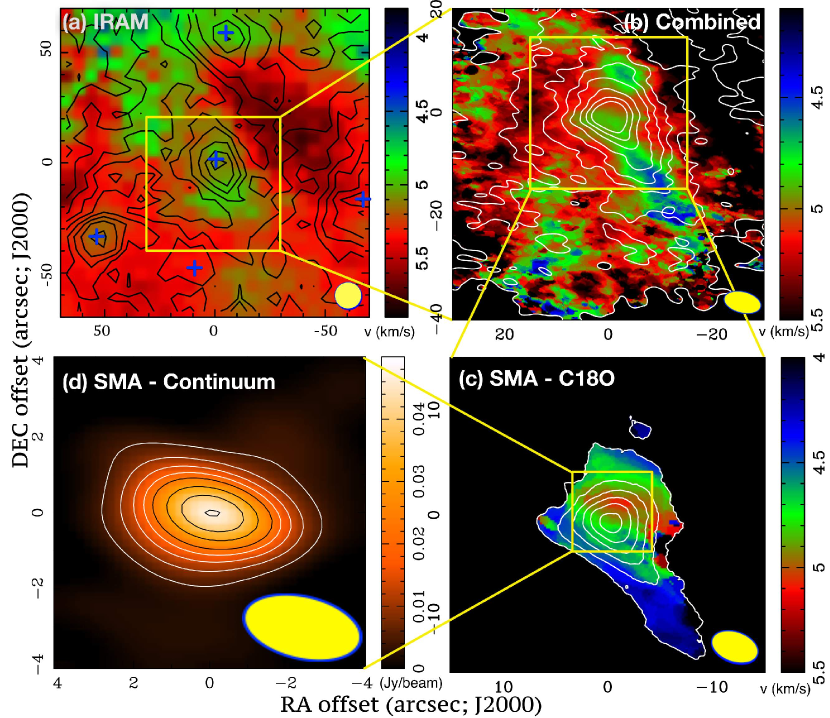
Figure 2.— (a) IRAM-30m C¹⁸O (2–1) single-dish moment 0 map (contour) overlaid on the moment 1 map (color) around L1455 IRS1. (b) As in (a) but for the SMA-IRAM-combined data, zooming in onto the yellow square in (a). (c) As in (a) but for SMA C¹⁸O (2–1). (d) SMA 1.3mm continuum map. A filled ellipse in the bottom right corner in each panel denotes the beam size. Crosses show the protostellar positions. Contour levels are from 5$\sigma$ in steps of 5$\sigma$ in (a) and from 3$\sigma$ in steps of 3$\sigma$ in (c), where 1$\sigma$ is 0.034 K km s^-1 in (a) and 100 mJy beam^-1 km s^-1 in (c), respectively. Contours start from 3$\sigma$ in steps of 3$\sigma$ in (b), where 1$\sigma$ is 92 mJy beam^-1 km s^-1, and contours are 3$\sigma$ to 15$\sigma$ in steps of 3$\sigma$, and then in 5$\sigma$ in (d), where 1$\sigma$ is 1.55 mJy beam^-1.

III.1.2 ¹²CO (2–1) Emission

Figure 3 displays the SMA ¹²CO (2–1) line emission in L1455 IRS1. A V-shaped structure is revealed in the red-shifted wing with an opening angle of $\sim$45^∘. The blue-shifted wing is also converging to the protostellar position, with a less pronounced geometry but a likely opening angle similar to its red-shifted counterpart. The blue-shifted wing extends to the southwest over $\sim 25^{\prime\prime}$ in length ($\sim$6250 AU). The shorter ($\sim 10^{\prime\prime}$) red-shifted wing is pointing to the northeast.

The ¹²CO emission likely outlines the collimated bipolar outflow as observed previously in H₂ (Davis et al., 1997a) and ¹²CO (3–2) with the JCMT (Curtis et al., 2010b). Their single-dish maps suggest a $\sim$40^∘ P.A. of the outflow axis, while the recent interferometric observation by Hull et al. (2014) with CARMA shows a slightly larger P.A. of $\sim$66^∘ (measured counter-clockwise from north). Our ¹²CO emission map with the SMA aligns closely with the CARMA result. We, therefore, adopt 66^∘ as the outflow axis P.A. in the following analyses.

Figure 3.— ¹²CO (2-1) moment 0 map with blue contours integrated from $v=−4.6$ km s^-1 to $v=3.8$ km s^-1 and red contours from $v=5.9$ km s^-1 to $v=14.4$ km s^-1. A filled ellipse in the bottom right corner denotes the synthesized beam size. A cross shows the protostellar position. Contour levels are from 3$\sigma$ in steps of 3$\sigma$, where 1$\sigma$ is 1 Jy beam^-1 km s^-1.

III.1.3 C¹⁸O (2–1) Emission

Figure 2(c) shows the integrated-intensity (i.e., moment 0) map (contours) overlaid on the intensity-weighted mean velocity (i.e., moment 1) map (color) of the C¹⁸O (2–1) emission in L1455 IRS1. Generally, the emission delineates a compact morphology with a size of $\sim$1000 AU. The emission above 6$\sigma$ shows a clear velocity gradient perpendicular to the ¹²CO (2–1) outflow axis (Figure 3). A two-dimensional Gaussian is fitted to the central compact region with intensity $>5\sigma$ giving a deconvolved size of $\sim 6^{\prime\prime}$. Furthermore, another velocity gradient is present in the northwestern part, with a gradient opposite to the one across the innermost region. A protrusion extending toward the southwest is lying approximately perpendicularly to the larger-scale velocity gradient. Given its direction that is roughly aligned with the outflow axis, this could be an outflow contamination. A second smaller protrusion is found to the north.

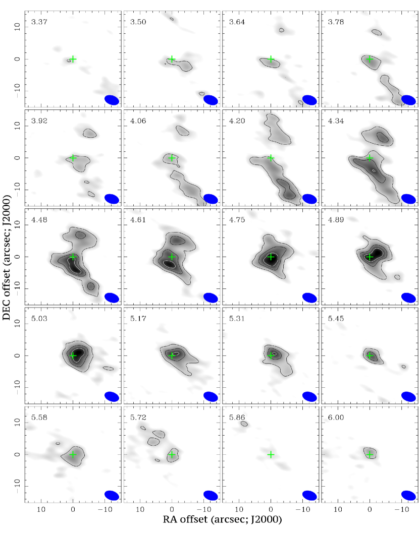
Figure 4.— SMA velocity channel maps of C¹⁸O (2–1) emission in L1455 IRS1 (two channels binned). The velocity of each channel is shown in the upper left corner in each panel. A filled ellipse in the bottom right corner in each panel denotes the beam size. Crosses show the IRS1 protostellar position. Contour levels are from 3$\sigma$ in steps of 3$\sigma$, where 1$\sigma$ is 115 mJy beam^-1.

Figure 4 shows the SMA velocity channel maps of C¹⁸O (2–1) centered on L1455 IRS1. We bin two channels for higher signal-to-noise ratio. 20 channels have a maximum emission above a 3$\sigma$ level, with velocities ranging from $3.26$ km s^-1 to $6.13$ km s^-1. At velocities $\lesssim 4.8$ km s^-1, the emission indicates a compact object located south to the protostellar position. In the range $4.8\lesssim v\lesssim 5.3$ km s^-1, this emission is shifted north. Around the systemic velocity of about 4.7 km s^-1, the emission stretches to the north and the southwest, along the outflow axis. For velocities larger than $\sim$5.3 km s^-1, however, the emission shows no significant spatial offsets. This demonstrates an asymmetrical velocity distribution along the possible rotational axis, likely due to the two protrusions joining the compact object from the north and the west.

III.2. IRAM - C¹⁸O (2–1) Emission

Figure 2(a) displays moment 0 and moment 1 C¹⁸O (2–1) overlaid maps observed with the IRAM-30m telescope. The map includes the central protostar L1455 IRS1, and partly covers two more protostars, L1455 IRS4 and IRS5, and two possible starless cores, HRF40 (Hatchell et al., 2007; Curtis et al., 2010a) and CoreW (this paper). We present C¹⁸O (2–1) velocity channel maps (5 channels are binned for presentation) in Figure 5. In the regions between the cores, significant emission is detected that appears to form filamentary structures and bridges connecting the individual cores. The central component observed in the moment 0 map is best described by a core size of $\sim 40^{\prime\prime}$ from two-dimensional Gaussian fitting.

Figure 5.— IRAM-30m C¹⁸O (2–1) velocity channel maps around L1455 IRS1 (five channels binned). The central velocity of the five binned channels is shown in the upper left corner in each panel. A filled circle in the bottom right corner in each panel denotes the beam size. Red crosses show the protostellar position of L1455 IRS1, green ones indicate the positions of IRS4, IRS5, HRF40, and CoreW. A blue box in the middle left panel indicates the location of the filamentary structure in between IRS1 and HRF40. Contour levels are from 3$\sigma$ in steps of 3$\sigma$, where 1$\sigma$ is 0.107 K.

Multiple velocity components can be seen at and connecting to the locations of L1455 IRS4 and IRS5. At the location of IRS4, a first component around $v\sim 4.8$ km s^-1 is likely a protostellar core, whereas a second component around $v\sim$5.8 km s^-1 might correspond to a larger structure which extends to the southwest. Indeed, most studies in the literature measure a systemic velocity for L1455 IRS4 of $\sim$4.9 km s^-1, and not 5.8 km s^-1 (Juan et al., 1993; Kirk et al., 2007; Friesen et al., 2013). Towards L1455 IRS5, a bridge protruding from CoreW can be readily seen from $v\sim 5.5$ km s^-1 to $\sim 6.2$ km s^-1. From JCMT ¹³CO observations (Curtis et al., 2010a), this bridge appears to be linked to IRS5 because it doest not stretch further across its position. However, a second more compact and uniform (in shape) component with a centroid velocity of $\sim$4.4 km s^-1 lies on the IRS5 protostellar position as well.

L1455 IRS1 appears to be marginally elongated along a north-south axis. A unique velocity gradient linking IRS1 and HRF40, with a P.A. $\sim$164^∘, occurs from $v\sim 4.8$ km s^-1 (IRS1) to $\sim$5.0 km s^-1 (Section V.2). In the IRAM-30m C¹⁸O emission, this is the only manifest large-scale structure that is connected with IRS1 in both space and velocity. Although clear in velocity, it is mixed spatially with surrounding structures, particularly the triangular zone around IRS1. The SMA C¹⁸O emission shows no clear corresponding structure, implying that this large-scale structure is either resolved out by the SMA or it is not associated with the inner structures directly.

III.3. SMA-IRAM-Combined C¹⁸O (2–1) Emission

Figure 6 shows the flux comparison for the C¹⁸O (2–1) emission in the central $5\farcs 6\times 5\farcs 6$ region from the SMA, IRAM-30m, and the SMA-IRAM-combined maps. The SMA has about 70% missing flux in velocities $\gtrsim$4.8 km s^-1. The combined map recovers roughly all the flux as observed by the IRAM-30m.

The SMA-IRAM-combined moment 0 and moment 1 maps of C¹⁸O (2–1) are overlaid in Figure 2(b). In the innermost region, the velocity gradient perpendicular to the outflow direction seen in the SMA-only map (Figure 2(c)) is still present but less distinct. The large gradient seen in the IRAM-only map extending to the south (from IRS1 to HRF40, Section V.2) can be seen in the combined map as the blue-green region connecting towards the central SMA component. While both gradients are observed in the combined map, it is obvious that the combination process has added more detailed information that, in this case, tends to blur features that are clearly detected in the SMA- and IRAM-only maps. This is explained by noticing that the IRS1 disk and the filament are well captured by the separate scales probed by the SMA and IRAM-30m, respectively. This is not obvious from the beginning and will generally depend on a source size and its distance. Additionally, the combined map demonstrates that there are only smaller-scale but no coherent larger-scale structures that could bias identification and interpretation of the large filament connecting towards IRS1 (Section V.2).

Figure 6.— C¹⁸O (2–1) spectra in the central $5\farcs 6\times 5\farcs 6$ (IRAM central pixel) of L1455 IRS1 with respect to velocity. The solid red curve shows the spectrum of the SMA-IRAM-combined map. The blue dashed and orange dotted curves are the IRAM- and SMA-only spectra.

IV. Analysis

IV.1. Position-Velocity Diagrams: Rotation in L1455 IRS1

Figure 7.— Left panels: Comparison between the SMA 1.3 mm continuum (black) and the SMA blue- and red-shifted C¹⁸O (2-1) emission. Right panels: Corresponding images of the Keplerian model. (a) High-velocity emission, (b) low-velocity emission. The velocity ranges (relative to $V_{\text{sys}}$) are 0.7–1.0 km s^-1 and $<0.7$ km s^-1 for high- and low-velocity, respectively. The continuum beam is shown at the bottom left corner. The larger ellipse shows the beam size for the C¹⁸O emission. Crosses show the protostellar position. Contour levels are from 5$\sigma$ in steps of 5$\sigma$ for continuum, 2$\sigma$ for C¹⁸O (2-1).

YSOs evolve via accreting material. The usually accompanying outflows are believed to be the removal mechanism for excessive angular momentum (e.g., McKee & Ostriker (2007)). Due to the distinct outflows in L1455 IRS1, detected in ¹²CO (2–1) (Figure 3), we expect that the core is also associated with a disk that we assume to be rotating in a plane orthogonal to the outflow axis. The optical depth of the C¹⁸O (2-1) emission in L1455 IRS1 is estimated to be $\sim 0.2$ on average in a velocity channel in the central 2${}^{\prime\prime}\times 2^{\prime\prime}$ region of the combined map, where the excitation temperature is taken to be 12.6K (Curtis et al., 2010a). The emission is, thus, optically thin and tracing the innermost parts in the envelope. In conclusion, the C¹⁸O (2-1) emission is indicative of the motions near the protostar.

The left panel in Figure 7(a) presents a comparison between the 1.3 mm continuum and the high-velocity C¹⁸O (2–1) emission. The blue- and red-shifted high-velocity components and the protostar are well aligned along the axis perpendicular to the outflow direction, hinting the existence of a rotational motion. Figure 8 displays Position-Velocity (P-V) diagrams of the C¹⁸O (2-1) emission of the SMA map of L1455 IRS1. The center of the P-V diagrams is the protostellar position. The P-V cuts are along P.A.$=66^{\circ}$ in Figure 8(a), and P.A.$=156^{\circ}$ in Figure 8(b), which are the angles along and perpendicular to the outflow axis (see section III.1.2).

Figure 8.— Position-Velocity diagrams of the C¹⁸O (2–1) SMA map of L1455 IRS1, (a) along and (b) perpendicular to the outflow axis. The absence of velocity gradients in (a) implies the absence of non-rotational motions along the radial direction of the disk. The blue and red points in (b) stand for blue- and red-shifted velocities with respect to the systemic velocity. Contour levels are from 3$\sigma$ in steps of 1$\sigma$, where 1$\sigma$ is 115 mJy beam^-1.

Since the line-of-sight velocity of a purely rotating disk is zero along the minor axis, any velocity variation along this axis must be non-rotational. In other words, the velocity profile along the minor axis can be a measure for infalling motions or outflow contamination. If there is infalling motion, we expect a velocity gradient along the minor axis. Therefore, the lack of a significant velocity gradient in Figure 8(a) suggests that there is no clear infalling motion in IRS1. On the other hand, for any disk that is not face-on, i.e., with an inclination angle different from $90^{\circ}$, the velocity profile along the major axis represents rotational disk features. Thus, we are aiming at measuring velocity profiles as a function of rotational radius along each axis. Figure 8(b) infers a differential velocity increase from larger to smaller rotational radii. Combining these findings, we conclude on the existence of a dominant rotating structure in this region (e.g., Belloche (2013)). We quantify this rotation in the subsequent section, following the technique outlined in Yen et al. (2013).

We note that because of asymmetric envelope features (see Section IV.3 below), it is difficult to reproduce all the observed patterns with a simple model. As we will show in section IV.3, these structures cannot be described by a flat disk model. In the P-V diagrams described here, most of these structures either lie outside of the diagram (i.e., located at $>5^{\prime\prime}$ from the center), or they are much weaker in terms of emission intensity as compared to the rotational feature.

IV.2. Existence of Disk

We assume a velocity profile for rotation that follows a power law

$$v_{\text{rot}}(r)\propto r^{p},$$ (2)

where $v_{\text{rot}}$ is the rotational velocity at a radius $r$, and $p$ is the power law index. Projected on the plane-of-sky, $p$ does not change, but the rotational velocity and radius are replaced by the projected relative velocity ($\equiv V$) and positional offset in the P-V diagram. We, thus, fit the representative points in Figure 8(a) with Equation (2) to derive $p$ and measure the disk rotation.

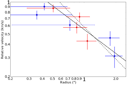
Figure 9.— Projected velocity profile of L1455 IRS1 as a function of radius $r$ in log-log scale. Blue and red points stand for blue- and red-shifted velocities with respect to the systemic velocity. The best-fit power law index is $p=-0.75\pm 0.16$ with a systemic velocity $V_{sys}=4.70$ km s^-1 (black solid line). The black dashed line indicates the best-fit result for a fixed value $p=-1$ for the outer 6 points.

The systemic velocity is found by fitting Gaussian profiles to the spectra used for Figure 6. The SMA and IRAM-30m spectra give 4.70 km s^-1 and 4.99 km s^-1, respectively. This implies that the two maps are tracing different gas components. This further explains why rotation is not evident in the combined map in Figure 2(b). The larger scale components with higher velocities in the IRAM-30m map are likely structures that are not directly associated with the inner rotating SMA component. Consequently, components from outer regions cannot be used to analyzing rotation. We, therefore, do not include the IRAM-30m map for more outer data points in the P-V diagrams, and we consider only the SMA map be tracing the rotational motion in the inner region. Hence, the systemic velocity ($\equiv V_{\text{sys}}$) is fixed to 4.70 km s^-1. Error bars in velocities are set to be the channel width.

To determine the profile, we fit a Gaussian in each velocity channel to get a centroid position which is then regarded as the rotational radius at that rotational velocity. A two-dimensional orthogonal distance regression is applied to find the best-fit parameters as shown in Figure 9. As a result, the observed motion can be best represented by a power law with $p=-0.75\pm 0.16$. This suggests that the rotational features seen in the P-V diagram are likely caused by a spin-up rotation.

Observations show that protostellar disks can possess two distinct motions (e.g., Murillo et al. (2013); Yen et al. (2015)): infalling (and rotating) motion with conserved angular momentum ($p=-1$), and pure Keplerian rotation ($p=-0.5$). A power law index in between these two values is possibly caused by insufficient instrumental resolution, blending the two types of motion and rendering them indistinguishable (e.g., Lee (2010)). Indeed, flattened inner data points can be seen in the velociy profile. This is also observed in L1527 IRS, and possibly indicates the existence of such a transition (Ohashi et al., 2014). To provide further evidence, we fit another power law only to the outer 6 points, obtaining an index of $-0.9\pm 0.3$, which is suggestive of an infalling (and rotating) envelope with conserved angular momentum. Thus, assuming the rotation indeed has a constant angular momentum, we force $p=-1.0$ and fit for the outermost 6 data points. The result is shown in Figure 9, likely hinting the presence of a Keplerian disk with a radius $\lesssim 0\farcs 8$ ($=$200AU) in IRS1. We note that this radius is consistent with the deconvolved size of the SMA 1.3mm continuum image (Section III.1.1), and hence we adopt a disk radius of 0$\farcs$8. As will be discussed below, the inclination angle of L1455 IRS1 is likely in the range of $22.5^{\circ}$ to $67.5^{\circ}$. Assuming it to be $45^{\circ}$, the best-fit profile gives a specific angular momentum $j=(1.0\pm 0.09)\times 10^{-3}$ km s^-1 pc. Moreover, for the inner disk radius of $0\farcs 8$, the protostellar mass ($\equiv M_{\ast}$) can be calculated following Keplerian motion, $v_{\text{rot}}=\sqrt{GM_{\ast}/r}$, which gives $M_{\ast}=(0.28\pm 0.05)M_{\sun}$.

IV.3. Asymmetric Envelope Features

In section IV.2, we conclude that the rotation in L1455 IRS1 is hinting a disk that is likely of Keplerian nature in its inner part. In this section, we further examine the properties of the envelope of L1455 IRS1. We construct a simple Keplerian disk model, which is parametrized by four physical quantities: inclination angle ($\equiv i$), position angle of the major axis ($\equiv\theta$), two-dimensional intensity distribution on the plane-of-sky, and rotational velocity distribution. Since the red- and blue-shifted wings of the ¹²CO (2-1) outflow do not overlap spatially except for the central compact structure, the permitted range of inclination angles can be inferred based on geometrical arguments. Figure 10 illustrates the ideas. Suppose the outflow wings are perfect cones. Hence, the opening angle projected on any plane is the same as that on the plane-of-sky. From the geometry of the integrated intensity map, the opening angle is estimated to be about $45^{\circ}$. By noticing that the outflow axis is orthogonal to the disk major axis, the inclination angle can be constrained from the distribution of red- and blue-shifted emission on the plane-of-sky. The wings start to overlap in velocity (Figure 10(b)) if the disk is nearly edge-on, i.e., $i\geqslant 90^{\circ}-45^{\circ}/2=67.5^{\circ}$. They are spatially overlapped along the line-of-sight (Figure 10(c)) if $i\leqslant 45^{\circ}/2=22.5^{\circ}$. Otherwise the two wings are completely separated, both in terms of spatial distribution and velocity (Ulrich, 1976).

Figure 10.— Schematics of outflow wings. The opening angle projected on the plane is $\sim 45^{\circ}$. (a) The observed outflows show two distinctive separate wings, red- and blue-shifted. (b) If $i$ is larger than $67.5^{\circ}$, each wing shows both red- and blue-shifted emission. (c) The wings near the central part on the plane-of-sky overlap. They, thus, appear as overlapping red- and blue-shifted emission in the central region, if $i$ is less than $22.5^{\circ}$.

We set $i=45^{\circ}$, because the geometrical appearance of the C¹⁸O (2-1) moment 0 map (Figure 2(b)) is neither round nor thin, and the red- and blue-shifted emission barely overlap in the central part. Specific angular momentum and protostellar mass are then $j=(1.0\pm 0.09)\times 10^{-3}$ km s^-1 pc and $M_{\ast}=0.28\pm 0.05M_{\sun}$ (Section IV.2). The slight overlapping of the red- and blue-shifted wings is likely due to insufficient spatial resolution, as a result of beam convolution. The position angle is fixed to $156^{\circ}$, as also used for the P-V diagrams. The deconvolved size of the two-dimensional Gaussian of the central part of the SMA C¹⁸O (2-1) integrated intensity map (Figure 2(c), Section III.1.3) is adopted as the intensity distribution for the disk model. By doing so, we assume that the disk is completely axisymmetric and most of the emission is dominated by the disk. With this, a simple Keplerian model is constructed with the MIRIAD tasks velmodel and velimage, where the rotational velocity profile is determined by the above $M_{\ast}$.

The results are illustrated in Figure 7. A comparison between observations and the model for high-velocity emission (Figure 7(a)) shows an overall consistency: The blue- and red-shifted high-velocity components are likely tracing the rotation of the inner Keplerian disk. On the other hand, the low-velocity channels (Figure 7(b)) present the asymmetric envelope: In both red- and blue-shifted components, an elongated structure lying approximately along the outflow direction can be seen. This feature is likely caused by outflow contamination. A northern clump extending along the disk major axis to $\sim 6^{\prime\prime}$ away from the protostellar position is evident in the blue-shifted channels. As mentioned in section III.1.3, this feature shows a velocity gradient inverse to the one across the disk. It, therefore, likely is independent of the rotating disk. These structures are, thus, features in the surrounding envelope, which cannot be explained by a simple Keplerian rotation.

V. Discussion

V.1. Fast Rotation in Small Core

Figure 11.— PV diagram of the IRAM C¹⁸O (2–1) emission along P.A.$=164^{\circ}$. The protostar L1455 IRS1 lies on the left side, whereas the peak on the right side is the starless core HRF40. A filamentary structure linking the two cores is marked by the magenta points, which indicate the velocity gradient along the filament. The velocity gradient is 8.1$\pm$0.8 km s^-1 pc^-1. The contours are from 3$\sigma$ to 9$\sigma$ in step of 1$\sigma$, where 1$\sigma$ is 0.156K.

To quantify rotation in the IRS1 core, we measure the centroid velocities of the core along P.A.$=156^{\circ}$ (i.e., along the disk major axis), by fitting Gaussian functions to the spectra at radii from 0 to $\sim 2000$AU in the IRAM-30m data. A linear velocity gradient is fitted to the profile, yielding (7.8$\pm$5.2) km s^-1 pc^-1. This gradient suggests a rotation with the same direction as the disk and envelope (Section IV). Assuming the core follows a rigid body rotation, the specific angular momentum $j$ amounts to $(4.6\pm 3.1)\times 10^{-3}$ km s^-1 pc, at the radius of the core (i.e., 5000AU, see Section III.2). Goodman et al. (1993) find a power-law relation between core sizes and specific angular momenta in complex dense cores, following $j=10^{-0.7\pm 0.2}R^{1.6\pm 0.2}$, where $j$ and $R$ are in units of km s^-1 pc and pc, respectively. Specifically, for a core similar in size to IRS1 ($R=5000$AU$\sim 0.024$pc), the relation predicts $j=(5.2\pm 4.5)\times 10^{-4}$ km s^-1. Tobin et al. (2011) have observed velocity gradients of $\sim 1$ km s^-1 pc^-1, perpendicular to outflow axes in typical Class 0 cores. These measured gradients indicate $j\sim 6\times 10^{-4}$ km s^-1 pc on a 5000AU scale, consistent with the relation of Goodman et al. (1993). Hence, our observed value is one order of magnitude larger than expected. This suggests that the core possesses an uncommonly large specific angular momentum for its size. As we discuss in the following section, the surrounding filamentary structure might be responsible for this larger than average momentum.

V.2. Connection to Large-Scale Filament

Figure 12.— (a) Measured velocity gradient as a function of position angle extending from IRS1. (b) Mass infalling rate along each position angle of the filament. Colored lines indicate the best-fit gradient and the corresponding mass infalling rate. Dark gray shaded areas show error bounds from the fitting. A projection effect of $45^{\circ}\pm 15^{\circ}$ is represented by the light gray area.

Figure 11 is the P-V diagram along the structure extending from L1455 IRS1 (Figure 5). This structure shows emission above $5\sigma$, with a linear gradient in the region between the two protostellar cores IRS1 and HRF40. We fit for centroid velocities at each positional offset to get a velocity profile. The extracted profile either changes sign in its slope (towards IRS1) or it flattens (towards HRF40). We interpret the linear section of the gradient as a filament of length $\sim 0.034$pc (e.g., Hacar & Tafalla (2011); Kirk et al. (2013)). Best-fit magnitudes of gradients along a range of position angles are displayed in Figure 12(a), with a peak around the P.A. connecting IRS1 and HRF40, which we adopt as the direction of the filament. The maximum gradient is 8.1 $\pm$ 0.8 km s^-1 pc^-1. If we suppose the filament is a cylinder with uniform density, with material flowing towards IRS1, we can deduce a mass inflow rate $\dot{M}$ as (e.g., Kirk et al. (2013))

$$\left(\frac{\dot{M}}{M_{\odot}\text{Myr}^{-1}}\right)=1.02\left(\frac{\nabla V}{\text{km s}^{-1}\text{ pc}^{-1}}\right)\left(\frac{M_{\text{fila}}}{M_{\odot}}\right)$$ (3)

where $\nabla V$ is the velocity gradient. $M_{\text{fila}}$ is the mass of the filament, which can be estimated by calculating a column density enclosed in the filament, as

$$\left(\frac{M_{\text{enc}}}{M_{\odot}}\right) =1.13\times 10^{-4}\mu_{\text{H${}_{2}$}}$$

$$\left(\frac{m_{\text{H}}}{\text{kg}}\right)\left(\frac{D}{\text{pc}}\right)^{2}\left(\frac{A}{\text{arcsec}^{2}}\right)\left(\frac{N(\text{H${}_{2}$})}{\text{cm}^{-2}}\right)$$ (4)

where the enclosed mass is denoted as $M_{\text{enc}}$. $m_{\text{H}}$ is the atomic weight of hydrogen, $D$ is the distance ($=$250pc), and $A$ is the enclosed area. $N$ indicates the column density of H₂. The abundance ratio of H₂ and C¹⁸O in the L1455 region is estimated to be $N(\text{H${}_{2}$})=1\times 10^{7}N(\text{C${}^{18}$O})$ (Curtis et al., 2010a; Lee et al., 2014). The mean molecular weight of gas, $\mu_{\text{H${}_{2}$}}$, is 2.7 per H₂ (Nishimura et al., 2015). Thus, the filament has a mass $M_{\text{fila}}=0.34M_{\odot}$, where we have adopted an excitation temperature of 12.6K (Curtis et al., 2010a).

Figure 12(b) illustrates the mass inflow rate (Equation 3) against different P.A. Along the filament, we find $\dot{M}=2.8$ M_⊙ Myr^-1. Since a velocity gradient is clearly detected over an extended spatial area, the filament is unlikely in the plane-of-sky or aligned with the line-of-sight. For a projection angle in the range between $30^{\circ}$ to $60^{\circ}$, the mass infalling rate is a few solar masses per Myr. On the other hand, the accretion rate towards IRS1 can also be inferred from the bolometric luminosity of the protostar if the gravitational energy of the infalling material is fully converted into radiation when reaching the star. This is given by $L_{\text{bol}}=GM_{\ast}\dot{M}/R_{\ast}$, where the subscripted asterisks denote quantities of the protostar, yielding

$$\dot{M}=3.20\times 10^{-2}\left(\frac{M_{\ast}}{M_{\odot}}\right)^{-1}\left(\frac{R_{\ast}}{R_{\odot}}\right)\left(\frac{L_{\text{bol}}}{L_{\odot}}\right).$$ (5)

For $L_{bol}$=3.6$L_{\odot}$ (Dunham et al., 2013) and $R_{\ast}\approx$ 3–5$R_{\odot}$ (Stahler et al., 1980), we have $\dot{M}\approx 1-2$ M_⊙ Myr^-1. This is on the same order as calculated for the large-scale filament. Therefore, the detected filament could be the reservoir and feeding source for the protostellar system, providing significant infalling material. Since the time scale of a typical Class $\mathrm{0}/\mathrm{I}$ protostars is $\sim 10^{5}-10^{6}$ Myr (e.g., André et al. (2000)), and the mass of the dense core is 0.54M_⊙, this mechanism, if maintained, can provide a similar amount of mass through the Class $\mathrm{0}/\mathrm{I}$ stages.

We can further estimate the kinetic energy of the infalling material as $E_{\text{k}}=M_{\text{fila}}V_{\text{inf}}^{2}/2$, where $V_{\text{inf}}$ is the weighted mean infalling velocity of the filament with respect to the systemic velocity. For $V_{\text{sys}}=4.70$ km s^-1 (Section IV.2), $V_{\text{inf}}=0.22$ km s^-1. On the other hand, assuming a constant specific angular momentum for the dense core in IRS1 and assuming the core to be an isothermal sphere, the rotational energy is $E_{\text{R}}=1/2I\omega^{2}$ where $\omega$ is the angular velocity of the rotating core and $I=2/9M_{\text{IRS1}}R^{2}$ is its moment of inertia, where the mass of the dense core ($\equiv M_{\text{IRS1}}$) encompassing L1455 IRS1 is 0.54M_⊙. The ratio of the two energies is then $E_{\text{k}}/E_{\text{R}}\sim 3.5$. This indicates that the filament is dynamically not negligible, but can possibly have significant impact on the core rotation. We note that $I\propto M_{\text{IRS1}}R^{2}$ can vary by a factor of a few for different mass distributions. In conclusion, the faster-than-average envelope rotation seen in L1455 IRS1 could be related to the feeding from the associated filament. In return, this could play a crucial role in the evolution of IRS1, by effectively adding extra angular momentum to its rotational motion.

V.3. Sample Trends: Competing Energies

Dust polarization observations in L1455 IRS1 reveal an alignment between magnetic (B) field and outflow axis on the core scale ($\sim$1pc), while the two axes become perpendicular on the envelope scale ($\sim$1000AU, Matthews et al. (2009); Hull et al. (2014)). MHD simulations show that such a change in field orientation can be due to the interplay between B-fields and gas motions (e.g., Machida et al. (2006)). Despite that such a change of orientations is seen in several sources (e.g., Hull et al. (2013, 2014)), unambiguous observational evidence to connect this to gas motions remains scarce (e.g., Yen et al. (2015)). Nevertheless, with the increasing resolution in the study of gas kinematics in Class 0, 0/I sources (e.g., Choi et al. (2010); Murillo et al. (2013); Ohashi et al. (2014)), the relation between B-fields and dynamics in protostars can now be discussed more systematically. To that purpose, we compile a sample of Class 0, 0/I protostars where sufficient data – from large and small scales, and from magnetic field morphologies – are available. We find 8 sources that satisfy these criteria (Table V.3). We choose 5 cores (L1455 IRS1, L1448 IRS2, L1448 IRS 3B, L1157 mm, L1527 IRS) which have both single-dish and interferometric data. Three addtional sources are selected that show either resolved disks (NGC1333 IRAS 4A and VLA 1623A) or a clear hint of the presence of a rotating disk (L1448 mm). All 8 sources have polarization observations. In Section V.3.1, we exemplify our analysis on L1455 IRS1 and discuss possible implications on its disk formation. Sample trends are presented in Section V.3.2.

Table 2Source Sample

Source	Protostellar Position		Distance	$L_{\text{bol}}$	$T_{\text{bol}}$	Reference
(Class)	(J2000)		(pc)	($L_{\sun}$)	(K)
L1455 IRS1	03h27m39s1	30∘13${}^{\prime}03\farcs 0$	250	3.6	65	1,2
(0)
L1448 IRS2	03h25m22s4	30∘45${}^{\prime}13\farcs 3$	250	2.1	53	2,3
(0/I)
L1448 IRS 3B	03h25m36s3	30∘45${}^{\prime}14\farcs 9$	250	4.3	90	2,3
(0/I)
L1157 mm	20h39m06s2	68∘02${}^{\prime}16\farcs 6$	250	4.1	35	2,3
(0)
L1527 IRS	04h39m53s9	26∘03${}^{\prime}09\farcs 8$	140	2.8	56	2,4
(0/I)
NGC1333 IRAS 4A	03h29m10s4	31∘13${}^{\prime}32\farcs 5$	250	4.2	51	2,3
(0)
L1448 mm	03h25m38s9	30∘44${}^{\prime}05\farcs 4$	250	4.4	69	2,3
(0)
VLA 1623A	16h26m26s4	-24∘24${}^{\prime}30\farcs 7$	120	1.1	10	5,6
(0)

References. — (1) This work; (2) Yen et al. (2015); (3) Enoch et al. (2009); (4) Tobin et al. (2011); (5) Murillo et al. (2013); (6) Murillo & Lai (2013)

V.3.1 Magnetic Field vs. Rotation: Change of Field Orientation Exemplified on L1455 IRS1

Based on ideal MHD equations under strict flux-freezing conditions, the B-field strength $B$ is found to be $\propto n^{2/3}$ (Mestel, 1966), where $n$ is the gas volume density. The B-field strength is estimated to be $\sim 5$ mG in the low-mass star forming region NGC1333 IRAS 4A, where n(H₂)$=4.3\times 10^{7}$ cm^-3 (Girart et al., 2006). Adopting this as a typical value for Class 0, $\mathrm{0}/\mathrm{I}$ sources, we deduce the field strengths in IRS1 according to the power law relation:

$$\left(\frac{B}{\text{$\mu$G}}\right)=2.6\times 10^{-2}\left(\frac{n(H_{2})}{\text{cm}^{-3}}\right)^{2/3}.$$ (6)

We note that with this scaling we are able to reproduce field strength values similar to Zeeman measurements (Troland & Crutcher, 2008) for the clouds ($\sim$0.5 pc) embedding NGC1333 IRAS 4A, L1455 IRS1, and L1448 IRS2, IRS 3B. Likewise, the observational estimate on a $\sim$1000 AU scale in L1157 mm (Stephens et al., 2013) also shows agreement. From Equation 6, we can calculate the B-field energy $E_{\text{B}}=VB^{2}/8\pi$, where $V$ is the volume. In the previous section, we have computed kinetic and rotational energies for the filament and the rotating core. Moreover, the rotational energy of a Keplerian disk can be expressed as $E_{\text{R}_{\text{d}}}=2j_{\text{d}}^{2}M_{\text{d}}/R_{\text{d}}^{2}$ assuming a uniformly distributed disk mass $M_{\text{d}}$, where $j_{\text{d}}$ is the specific angular momentum at the disk edge of radius $R_{\text{d}}$. With this, we find that the ratio $E_{\text{B}}/E_{\text{R}}$ changes from 3–4 on the filament/core scale to $E_{\text{B}}/E_{\text{R}_{\text{d}}}\sim 0.17$ on the disk scale (Table 3). Thus, the significance of the magnetic fields towards smaller scales evolves from dominant to minor. This hints that the rotational motion starts to be more important than the B-field in the innermost region where the disk is present. This supports the scenario that initially parallel field lines are dragged and bent by the rotating disk, and aligned along the disk major axis.

V.3.2 Sample Analysis: Changes from Core to Disk Scale

In this section, we inspect whether there are common trends among the 8 Class 0, $\mathrm{0}/\mathrm{I}$ sources in our sample. The limited available data allow us only to compare energies on the two characteristic scales: disk (infalling envelope) and core. Additionally, since the role of gravity is ignored in the previous discussion, we proceed to also compare B-field and rotational energy with gravitational energy. We assume uniform mass distributions on each scale and rigid-body rotation for cores. The energies on the core scale are calculated in a shell with the outer radius being the core radius, and the inner one being much larger than the rotating disk. This division ensures that inner spin-up motions as well as higher densities in the innermost regions do not mimic or overweigh any core dynamics at larger scales that are relevant in our comparison. The rotational and gravitational energies for disk and core are, therefore, given by

$$\left\{\begin{matrix}E_{\text{R}_{\text{d}}}=&\frac{2j_{\text{d}}^{2}M_{\text{d}}}{R_{\text{d}}^{2}}=\frac{2GM_{\ast}M}{R}\\ E_{\text{R}_{\text{c}}}=&\frac{1}{2}I\omega^{2}=\frac{1}{2}\frac{M_{\text{enc}}(R_{\text{c}}^{2}+R_{\text{m}}^{2})}{2}\frac{j_{\text{c}}^{2}}{R_{\text{c}}^{4}}\end{matrix}\right.$$ (7)

where the subscripts ’d’ and ’c’ denote values for disk and cores, respectively, and $R_{\text{m}}$ is the inner radius of the shell, and

$$\left\{\begin{matrix}E_{\text{G}_{\text{d}}}=&\frac{3}{2}\frac{GM_{\ast}M_{\text{d}}}{R_{\text{d}}}+\frac{3}{5}\frac{GM_{\text{d}}^{2}}{R_{\text{d}}}\\ E_{\text{G}_{\text{c}}}=&\frac{G(M_{\text{m}}+M_{\ast})}{R_{\text{c}}}M_{\text{enc}}\end{matrix}\right.$$ (8)

where the energy is added from both self-gravitating potential and the central protostar, and $M_{\text{m}}+M_{\ast}$ is the total mass encompassed by the inner shell radius (gas and star), for the total gravitational energy exerted on the shell by all the mass inside. The B-field energies $E_{B}$ are computed in the same way as in the previous section.

Figure 13.— Energy comparisons on disk and core scales in Class 0, $\mathrm{0}/\mathrm{I}$ sources. The gray-shaded region indicates the disk (envelope) scale ($<1000$ AU), and the right-half is the core scale. The error bars are obtained by adopting a factor of two uncertainties in $E_{B}$ and $M$ (e.g., $M\cdot 2^{\pm 1}$), and assuming equal uncertainties in $M$ for all energies.

The results are summarized in Table 3, Table Protostar L1455 IRS1: Rotating Disk Connecting to Filamentary Network and illustrated in Figure 13. Generally, the energy ratio $E_{B}/E_{R}$ shows a decline from core to disk scale, consistent with what we find for IRS1, i.e., the rotational energy gains in significance from large to small scale, where it can be comparable or dominating over the B-field energy. On the contrary, $E_{B}/E_{G}$ looks generally flat, with most values smaller than one. This trend probably indicates that we are not yet tracing the even larger scales where the B-field could be dominating and preventing collapse. Finally, we see an increasing importance of rotational energy as compared to gravitational energy with smaller scales. In particular, we note that, on the disk (envelope) scale, $E_{R}/E_{G}\sim 1$, which conforms with the expectation that the disks are rotationally supported and thus, prevent further infalling motions.

Finally, we note that, in our calculations we have assumed that B-field strengths scale following Equation 6), cores follow a rigid-body rotation, and mass is uniformly distributed. Although we have seen that the B-field strengths from independent observations give roughly the same values (Section V.3.1), the uncertainties can still be very large, and they are non-trivial to estimate. Therefore, besides uncertainties given by fitting results of rotations (i.e., for $j$), we include another factor of two uncertainties for $E_{B}$ and $M$, assuming that all the mass estimates are correlated, i.e., identical mass uncertainties apply to all energies. They are depicted in Figure 13 as error bars. While some sources show large error bars extending to zero, general trends are still apparent even in the presence of these large uncertainties.

VI. Summary and Conclusion

We present new SMA and IRAM-30m single-dish observations toward the Class 0/I protostar L1455 IRS1 and its surrounding. Our main results are summarized in the following.

1. SMA High-Resolution Observations. The SMA 1.3 mm continuum observation with a resolution of about $3^{\prime\prime}$ reveals a compact dust component centered on IRS1 with a size around 300 AU. Its mass is estimated to be about $0.01M_{\odot}$. With a spatial and velocity resolution around $4^{\prime\prime}$ and 0.069 km s^-1 in C¹⁸O (2–1), a clear velocity gradient of $\sim$150 km s^-1 pc^-1 is detected over a compact component of 1500 AU. A clear outflow perpendicular to this gradient is seen in ¹²CO, extending out to about 6000 AU. Additionally seen asymmetric features probably belong to a larger-scale envelope.

2. IRAM-30m Larger-Scale Observation. With a resolution of about $12^{\prime\prime}$, the IRAM-30m observation in C¹⁸O (2–1) over an area of about 0.2-by-0.2 pc captures the surroundings of IRS1 and partly also includes the protostars IRS4 and IRS5, and the starless cores HRF40 and CoreW. A network of complex structures, possibly bridges and filaments, in between these cores is apparent in the channel maps. IRS1 is found embedded in a dense core of about 0.05 pc in size with $0.35M_{\odot}$.

3. Rotation and Disk in L1455 IRS1. The C¹⁸O (2–1) emission towards IRS1 is optically thin, thus tracing the motion near the protostar. The lack of a clear gradient along the outflow direction in the P-V-diagram rules out significant infall motion. Fitting of the velocity gradient over the full range in the P-V-diagram perpendicular to the outflow direction is consistent with a rotational motion $v\sim r^{p}$ with a power-law index $p=-0.75$. Due to the limited instrumental resolution and the resulting blending of motions, this is likely indicative of a spin-up rotation, transitioning between an outer infalling and rotating motion with conserved angular momentum (observed with $p=-1$ when restricting the fitting to the largest scales, $\sim 300$ to 500 AU, in the P-V-diagram) and the innermost detected scales between 100 to 200 AU where the slope of the velocity profile flattens. All this hints the likely presence of a Keplerian disk with a radius smaller than 200 AU and a protostellar mass of $0.28M_{\odot}$.

4. Core Rotation and Filament Connection. A velocity gradient of about 8 km s^-1 pc^-1 is found from the IRAM-30m C¹⁸O (2–1) emission over the core scale. Assuming the IRS1 core follows a rigid-body rotation, this leads to a specific angular momentum of about $5\times 10^{-3}$ km s^-1 pc at the core radius around 5000 AU. This is about one order of magnitude larger than expected from a core-size-momentum scaling relation. Significant emission and structure is detected between the two cores IRS1 and HRF40. Probing a range of directions around IRS1 shows a maximum velocity gradient of 8 km s^-1 pc^-1 precisely towards HRF40. Interpreting this as a gradient along the filamentary connection between the two cores yields a mass inflow of $\dot{M}=1.8$ M_⊙ Myr^-1, similar to the accretion rate onto IRS1 derived from its bolometric luminosity. The resulting kinetic energy of the inflowing material is significant, a few times the core’s rotational energy. The filament is, thus, dynamically important, a main gas reservoir and possibly responsible for the larger-than-average core rotation.

5. Magnetic Field and Trends in Class 0/I Protostar Sample. In IRS1 the observed magnetic field orientation changes from parallel to the outflow axis on core scale to perpendicular on disk scale. This can be explained by our measured core and disk rotational energy which, compared to the magnetic field energy, grows from minor on large scale to dominating on small scale. The disk rotation is, thus, significant enough to bend the field lines and align them with the disk velocity gradient. This growing importance of rotation on the disk scale is generally observed in our sample of 8 Class 0/I protostellar sources. Moreover, the ratio of rotational-to-gravitational energy grows across the entire sample from large to small scale, approaching unity on disk scale which is consistent with the expectation of rotationally supported Keplerian disks. The magnetic-to-gravitational energy ratio remains roughly constant, smaller than one, over our tested scales.

Table 3Energy Comparison in Class 0, 0/I Sources

Source	Scale	$E_{B}$/$E_{R}$	$E_{B}$/$E_{G}$	$E_{R}$/$E_{G}$	$\Delta\theta_{\text{core}}$	$\Delta\theta_{\text{env}}$
(Class)
L1455 IRS1	disk	0.17(0.13)	0.22(0.19)	1.3(1.3)	6∘	84∘
($\mathrm{0}/\mathrm{I}$)	core	4.5(6.9)	0.49(0.41)	0.11(0.18)
	filament	2.7(2.0)	–	–
L1448 IRS2	disk	0.56(0.42)	0.52(0.43)	0.92(0.91)	15∘	3∘
($\mathrm{0}/\mathrm{I}$)	core	147(191)	0.18(0.15)	0.0012(0.0018)
L1448 IRS 3B	disk	0.069(0.050)	0.077(0.064)	1.12(1.10)	82∘	79∘
($\mathrm{0}/\mathrm{I}$)	core	2.7(2.1)	0.16(0.13)	0.059(0.059)
L1157 mm	envelope	76(94)	1.4(1.2)	0.019(0.026)	14∘	3∘
($\mathrm{0}$)	core	1800(2900)	0.64(0.53)	0.00035(0.00061)
L1527 IRS	disk	0.61(0.46)	0.54(0.45)	0.90(0.90)	32∘	87∘
($\mathrm{0}/\mathrm{I}$)	core	1200(1100)	0.56(0.46)	0.00048(0.00054)
NGC1333 IRAS 4A	disk	1.1(0.86)	0.65(0.54)	0.58(0.57)	37∘	$\sim 90^{\circ}$
($\mathrm{0}$)	core	–	0.16(0.14)	–
L1448 mm	disk	0.52(0.33)	0.54(0.45)	1.0(1.2)	44∘	45∘
($\mathrm{0}$)	core	–	0.27(0.23)	–
VLA 1623A	disk	0.20(0.05)	0.26(0.21)	1.30(1.29)	60∘	83∘
($\mathrm{0}$)	core	–	0.18(0.15)	–

. .

Note. — The values in parentheses are the uncertainties assuming a factor of two uncertainties in $E_{B}$ and $M$, and including errors from $j$ (see Table Protostar L1455 IRS1: Rotating Disk Connecting to Filamentary Network). The field orientations on core and envelope scale, $\Delta\theta_{\text{core}}$ and $\Delta\theta_{\text{env}}$, are the weighted averages from Hull et al. (2014)

Appendix A Combining SMA and IRAM-30m data: Reliability Test

Figure 14.— Schematic flow chart to test combination process. An image with characteristics similar to our source is adopted as the real sky. The central black, red, and blue boxes denote the simulated observed images of the real sky. The bottom two are simulated SMA and single-dish images. The validity of the combination process is evaluated by the significance of the residual between combined and expected image.

In order to check if the combination process by which we generate SMA-IRAM-combined maps does not remove real structures nor create artificial ones, we simulate the process as described below. The idea is illustrated in Figure 14. First, we choose a map to represent the real sky. The real sky is then converted into a simulated SMA and a simulated single-dish image (denoted simulated 30m image in Figure 14). After this, the two simulated images are combined through the above outlined method. To assess the quality of this combined map, we generate another simulated image, which is the (simulated) observed map with a synthesized beam of size equal to that of the combined map. Finally, this (simulated) observed map is compared with the combined map.

Since size and geometry of a source will generally affect what the source looks like in interferometric maps, we use the moment 0 of the combined map (Figure 2(b)) as the real sky. Furthermore, we are assured that the simulation does not produce non-ignorable artificial structures, which were present in Yen et al. (2011) because of the gap between their single-dish and the SMA uv-coverages. To simulate observations of the SMA, we multiply the real sky by the primary beam response of the SMA and convolve it with the SMA synthesized beam. For the single-dish IRAM-30m, the real sky is convolved with the 30m beam and then resampled onto the Nyquist grid as the real 30m map ($5\farcs 602$). The combination of the two subsequently gives a ”combined synthesized beam”, which is used to simulate the observed map of the real sky (indicated by the dashed arrow in Figure 14).

Finally, the (simulated) observed map is subtracted from the combined map, giving an absolute residual map (Figure 15(c)). Dividing this residual map by the observed map gives a map in unit of percentage, showing how significant the relative difference is (Figure 15(d)). The results are shown in Figure 15. Except for the inner most region, the combined map is consistent with the observed map within a 1$\sigma$ difference. In regions where the intensity is greater than 6$\sigma$, we find less than 10% flux deviation.

Figure 15.— (a) Real sky chosen for simulation. (b) Simulated observed image (blue contours) overlaid on combined map (red contours). Contour levels are from 3$\sigma$ in steps of 3$\sigma$ in (a) and (b). (c) Residual of combined map, subtracting observed one from (b). Contour levels are in steps of 0.5$\sigma$ of the observed map. Dashed lines indicate negative values. (d) Percentage with respect to the observed map. Overlaid are the observed contours (blue). The region with intensity lower than 3$\sigma$ of the observed map is masked (blank region). Contour levels are -10%, 10%, and 20% respectively. A cross-hatched ellipse in the bottom right corner in each panel denotes the synthesized beam size.

In conclusion, the simulation assures that the combination of the SMA and the IRAM-30m maps is credible. We note that the best weighting for reproducing the best non-distorted image varies from case to case. Since uv-samplings and beam sizes determine how well structures are recovered in combined maps, one should be careful when combining multiple data sets for different sources, with varying structures. We note, however, that it is impossible to perfectly reproduce the real-sky structures, due to the same reasons. We believe that a $<$10% loss in the central region is acceptable, given that the SMA usually has the same level of uncertainty in flux.

Table 4Properties of Class 0, 0/I Sources

Source	$M_{\ast}$	$R_{\text{d}}$	R	$M_{\text{enc}}$	N(H2)	$\mathbf{B}$	$j$	$E_{B}$	$E_{R}$	$E_{G}$	Ref.
(Class)	($M_{\sun}$)	(AU)	(AU)	($M_{\odot}$)	($\times 10^{5}$)	(mG)	($\times 10^{-4}$)	($\times 10^{40}$)	($\times 10^{40}$)	($\times 10^{40}$)
					(cm${}^{-3})$		(km s-1 pc)	(erg)	(erg)	(erg)
L1455 IRS1	0.28	180	140	0.011	700	7.0	10(0.9)	14	79(56)	60(84)	1,2,3,4
($\mathrm{0}/\mathrm{I}$)			6125-4900	0.35	0.52	0.06	46(31)	40	8.7(13)	81(110)
			10000	0.34	0.81	0.08	–	44	16	–
L1448 IRS2	0.18	260	340	0.046	190	2.9	8.7(0.7)	37	65(46)	70(98)	2,3,4,5
($\mathrm{0}/\mathrm{I}$)			7750-4900	0.56	0.27	0.04	15(7.9)	50	0.34(0.43)	280(390)
L1448 IRS 3B	1.5	530	700	0.068	33	0.90	38(1.5)	30	440(310)	390(540)	2,3,4,5
($\mathrm{0}/\mathrm{I}$)			6125-4900	3.7	5.4	0.27	130(13)	890	330(240)	5500(7700)
L1157 mm	0.05	$<$5	370	0.13	430	5.0	$<$0.5(0.25)	140	1.8(2.2)	9.5(13)	2,5,6
($\mathrm{0}$)			4900-3500	0.22	0.49	0.05	2.1(1.5)	25	0.014(0.022)	39(54)
L1527 IRS	0.16	110	70	0.036	17000	60	5.2(0.6)	130	210(160)	240(330)	2,5,6
($\mathrm{0}/\mathrm{I}$)			4200-2750	0.71	2.3	0.16	4.1(1.1)	140	0.12(0.10)	250(340)
NGC1333 IRAS 4A	0.14	680	160	0.56	24000	74	15(0.5)	2300	2000(1400)	3500(4800)	2,3,4
($\mathrm{0}$)			5000	7.8	10	0.42	–	2300	–	14000(20000)
L1448 mm	0.21	150	110	0.11	15000	54	7.9(2.3)	380	730(660)	700(970)	2,3,4
($\mathrm{0}$)			6750	1.9	1.0	0.089	–	260	–	960(1300)
VLA 1623A	0.22	150	150	0.008	390	4.8	8.3(–)	8.1	41(29)	32(44)	3,4,7
($\mathrm{0}$)			14000	0.24	0.015	0.005	–	8.3	–	45(63)

Note. — The values in parentheses are the uncertainties assuming a factor of two uncertainties in $E_{B}$ and $M$, and including errors from $j$. Error bars for disk $j$ are half of the best-fit results in Yen et al. (2015)’s model. The radius is determined from the mean value of the FWHM size of disk or core. Estimation of $M$ and N(H₂) assumes the same abundance ratio as in L1455 IRS1.

References. — (1) This paper, (2) Yen et al. (2015), (3) Enoch et al. (2009), (4) Enoch et al. (2006), (5) H.-W. Yen, (private communication), (6) Motte & André (2001), (7) Murillo et al. (2013).

References

- André et al. (2000) André, P., Ward-Thompson, D., & Barsony, M. 2000, Protostars and Planets IV, 59
- André et al. (2010) André, P., Men’shchikov, A., Bontemps, S., et al. 2010, A&A, 518, L102
- Anglada et al. (1989) Anglada, G., Rodriguez, L. F., Torrelles, J. M., et al. 1989, ApJ, 341, 208
- Arce et al. (2010) Arce, H. G., Borkin, M. A., Goodman, A. A., Pineda, J. E., & Halle, M. W. 2010, ApJ, 715, 1170
- Baars et al. (1987) Baars, J. W. M., Hooghoudt, B. G., Mezger, P. G., & de Jonge, M. J. 1987, A&A, 175, 319
- Bachiller & Cernicharo (1986) Bachiller, R., & Cernicharo, J. 1986, A&A, 166, 283
- Bally et al. (1997) Bally, J., Devine, D., Alten, V., & Sutherland, R. S. 1997, ApJ, 478, 603
- Bally et al. (2008) Bally, J., Walawender, J., Johnstone, D., Kirk, H., & Goodman, A. 2008, The Perseus Cloud, ed. B. Reipurth, 308
- Beckwith et al. (1990) Beckwith, S. V. W., Sargent, A. I., Chini, R. S., & Guesten, R. 1990, AJ, 99, 924
- Belloche (2013) Belloche, A. 2013, in EAS Publications Series, Vol. 62, EAS Publications Series, ed. P. Hennebelle & C. Charbonnel, 25
- Bergin & Tafalla (2007) Bergin, E. A., & Tafalla, M. 2007, ARA&A, 45, 339
- C̆ernis (1993) C̆ernis, K. 1993, Baltic Astronomy, 2, 214
- Choi et al. (2010) Choi, M., Tatematsu, K., & Kang, M. 2010, ApJ, 723, L34
- Cohen (1980) Cohen, M. 1980, AJ, 85, 29
- Cox et al. (2015) Cox, E. G., Harris, R. J., Looney, L. W., et al. 2015, ApJ, 814, L28
- Curtis et al. (2010a) Curtis, E. I., Richer, J. S., & Buckle, J. V. 2010a, MNRAS, 401, 455
- Curtis et al. (2010b) Curtis, E. I., Richer, J. S., Swift, J. J., & Williams, J. P. 2010b, MNRAS, 408, 1516
- Davis et al. (1997a) Davis, C. J., Eisloeffel, J., Ray, T. P., & Jenness, T. 1997a, A&A, 324, 1013
- Davis et al. (1997b) Davis, C. J., Ray, T. P., Eisloeffel, J., & Corcoran, D. 1997b, A&A, 324, 263
- Davis et al. (2008) Davis, C. J., Scholz, P., Lucas, P., Smith, M. D., & Adamson, A. 2008, MNRAS, 387, 954
- de Zeeuw et al. (1999) de Zeeuw, P. T., Hoogerwerf, R., de Bruijne, J. H. J., Brown, A. G. A., & Blaauw, A. 1999, AJ, 117, 354
- Di Francesco (2012) Di Francesco, J. 2012, in Astronomical Society of India Conference Series, Vol. 4, Astronomical Society of India Conference Series, 13
- Di Francesco et al. (2007) Di Francesco, J., Evans, II, N. J., Caselli, P., et al. 2007, Protostars and Planets V, 17
- Dunham et al. (2014) Dunham, M. M., Arce, H. G., Mardones, D., et al. 2014, ApJ, 783, 29
- Dunham et al. (2013) Dunham, M. M., Arce, H. G., Allen, L. E., et al. 2013, AJ, 145, 94
- Enoch et al. (2009) Enoch, M. L., Evans, II, N. J., Sargent, A. I., & Glenn, J. 2009, ApJ, 692, 973
- Enoch et al. (2006) Enoch, M. L., Young, K. E., Glenn, J., et al. 2006, ApJ, 638, 293
- Evans et al. (2009) Evans, N. J. I., Dunham, M. M., Jørgensen, J. K., et al. 2009, The Astrophysical Journal Supplement Series, 181, 321
- Frerking et al. (1982) Frerking, M. A., Langer, W. D., & Wilson, R. W. 1982, ApJ, 262, 590
- Friesen et al. (2013) Friesen, R. K., Kirk, H. M., & Shirley, Y. L. 2013, ApJ, 765, 59
- Girart et al. (2006) Girart, J. M., Rao, R., & Marrone, D. P. 2006, Science, 313, 812
- Goldsmith et al. (1984) Goldsmith, P. F., Snell, R. L., Hemeon-Heyer, M., & Langer, W. D. 1984, ApJ, 286, 599
- Goodman et al. (1993) Goodman, A. A., Benson, P. J., Fuller, G. A., & Myers, P. C. 1993, ApJ, 406, 528
- Hacar & Tafalla (2011) Hacar, A., & Tafalla, M. 2011, A&A, 533, A34
- Hatchell et al. (2007) Hatchell, J., Fuller, G. A., Richer, J. S., Harries, T. J., & Ladd, E. F. 2007, A&A, 468, 1009
- Hatchell et al. (2005) Hatchell, J., Richer, J. S., Fuller, G. A., et al. 2005, A&A, 440, 151
- Helou & Walker (1988) Helou, G., & Walker, D. W., eds. 1988, Infrared astronomical satellite (IRAS) catalogs and atlases. Volume 7: The small scale structure catalog, Vol. 7
- Ho et al. (2004) Ho, P. T. P., Moran, J. M., & Lo, K. Y. 2004, ApJ, 616, L1
- Hull et al. (2013) Hull, C. L. H., Plambeck, R. L., Bolatto, A. D., et al. 2013, ApJ, 768, 159
- Hull et al. (2014) Hull, C. L. H., Plambeck, R. L., Kwon, W., et al. 2014, ApJS, 213, 13
- Johnstone et al. (2004) Johnstone, D., Di Francesco, J., & Kirk, H. 2004, ApJ, 611, L45
- Jørgensen et al. (2008) Jørgensen, J. K., Johnstone, D., Kirk, H., et al. 2008, ApJ, 683, 822
- Jørgensen et al. (2006) Jørgensen, J. K., Harvey, P. M., Evans, II, N. J., et al. 2006, ApJ, 645, 1246
- Jørgensen et al. (2007) Jørgensen, J. K., Bourke, T. L., Myers, P. C., et al. 2007, ApJ, 659, 479
- Juan et al. (1993) Juan, J., Bachiller, R., Koempe, C., & Martin-Pintado, J. 1993, A&A, 270, 432
- Kirk et al. (2007) Kirk, H., Johnstone, D., & Tafalla, M. 2007, ApJ, 668, 1042
- Kirk et al. (2013) Kirk, H., Myers, P. C., Bourke, T. L., et al. 2013, The Astrophysical Journal, 766, 115
- Kirk et al. (2005) Kirk, J. M., Ward-Thompson, D., & André, P. 2005, MNRAS, 360, 1506
- Lee (2010) Lee, C.-F. 2010, ApJ, 725, 712
- Lee et al. (2014) Lee, M.-Y., Stanimirović, S., Wolfire, M. G., et al. 2014, ApJ, 784, 80
- Levreault (1988) Levreault, R. M. 1988, ApJS, 67, 283
- Lynds (1962) Lynds, B. T. 1962, ApJS, 7, 1
- Machida et al. (2006) Machida, M. N., Matsumoto, T., Hanawa, T., & Tomisaka, K. 2006, The Astrophysical Journal, 645, 1227
- Matthews et al. (2009) Matthews, B. C., McPhee, C. A., Fissel, L. M., & Curran, R. L. 2009, ApJS, 182, 143
- McKee & Ostriker (2007) McKee, C. F., & Ostriker, E. C. 2007, ARA&A, 45, 565
- Mestel (1966) Mestel, L. 1966, MNRAS, 133, 265
- Motte & André (2001) Motte, F., & André, P. 2001, A&A, 365, 440
- Murillo & Lai (2013) Murillo, N. M., & Lai, S.-P. 2013, ApJ, 764, L15
- Murillo et al. (2013) Murillo, N. M., Lai, S.-P., Bruderer, S., Harsono, D., & van Dishoeck, E. F. 2013, A&A, 560, A103
- Nishimura et al. (2015) Nishimura, A., Tokuda, K., Kimura, K., et al. 2015, ApJS, 216, 18
- Ohashi et al. (2014) Ohashi, N., Saigo, K., Aso, Y., et al. 2014, ApJ, 796, 131
- Padoan et al. (1999) Padoan, P., Bally, J., Billawala, Y., Juvela, M., & Nordlund, Å. 1999, ApJ, 525, 318
- Piétu et al. (2007) Piétu, V., Dutrey, A., & Guilloteau, S. 2007, A&A, 467, 163
- Ridge et al. (2006) Ridge, N. A., Di Francesco, J., Kirk, H., et al. 2006, AJ, 131, 2921
- Sadavoy et al. (2010) Sadavoy, S. I., Di Francesco, J., Bontemps, S., et al. 2010, ApJ, 710, 1247
- Sancisi et al. (1974) Sancisi, R., Goss, W. M., Anderson, C., Johansson, L. E. B., & Winnberg, A. 1974, A&A, 35, 445
- Sargent (1979) Sargent, A. I. 1979, ApJ, 233, 163
- Sault et al. (1995) Sault, R. J., Teuben, P. J., & Wright, M. C. H. 1995, in Astronomical Society of the Pacific Conference Series, Vol. 77, Astronomical Data Analysis Software and Systems IV, ed. R. A. Shaw, H. E. Payne, & J. J. E. Hayes, 433
- Scoville et al. (1993) Scoville, N. Z., Carlstrom, J. E., Chandler, C. J., et al. 1993, PASP, 105, 1482
- Sepúlveda et al. (2011) Sepúlveda, I., Anglada, G., Estalella, R., et al. 2011, A&A, 527, A41
- Simon (2009) Simon, T. 2009, The Astrophysical Journal, 693, 1803
- Stahler et al. (1980) Stahler, S. W., Shu, F. H., & Taam, R. E. 1980, ApJ, 241, 637
- Stephens et al. (2013) Stephens, I. W., Looney, L. W., Kwon, W., et al. 2013, ApJ, 769, L15
- Sun et al. (2006) Sun, K., Kramer, C., Ossenkopf, V., et al. 2006, A&A, 451, 539
- Tafalla & Hacar (2015) Tafalla, M., & Hacar, A. 2015, A&A, 574, A104
- Tapia et al. (1997) Tapia, M., Persi, P., Bohigas, J., & Ferrari-Toniolo, M. 1997, AJ, 113, 1769
- Tobin et al. (2011) Tobin, J. J., Hartmann, L., Chiang, H.-F., et al. 2011, ApJ, 740, 45
- Troland & Crutcher (2008) Troland, T. H., & Crutcher, R. M. 2008, ApJ, 680, 457
- Ulrich (1976) Ulrich, R. K. 1976, ApJ, 210, 377
- Ungerechts & Thaddeus (1985) Ungerechts, H., & Thaddeus, P. 1985, in Bulletin of the American Astronomical Society, Vol. 17, Bulletin of the American Astronomical Society, 607
- Walker-Smith et al. (2014) Walker-Smith, S. L., Richer, J. S., Buckle, J. V., Hatchell, J., & Drabek-Maunder, E. 2014, MNRAS, 440, 3568
- Ward-Thompson et al. (2007) Ward-Thompson, D., André, P., Crutcher, R., et al. 2007, Protostars and Planets V, 33
- Wilson et al. (1996) Wilson, T. L., Gaume, R. A., Johnston, K. J., & Schmid-Burgk, J. 1996, in Science with Large Millimetre Arrays, ed. P. A. Shaver, 177
- Wu et al. (2007) Wu, J., Dunham, M. M., Evans, II, N. J., Bourke, T. L., & Young, C. H. 2007, AJ, 133, 1560
- Yen et al. (2015) Yen, H.-W., Koch, P. M., Takakuwa, S., et al. 2015, ApJ, 799, 193
- Yen et al. (2011) Yen, H.-W., Takakuwa, S., & Ohashi, N. 2011, ApJ, 742, 57
- Yen et al. (2013) Yen, H.-W., Takakuwa, S., Ohashi, N., & Ho, P. T. P. 2013, ApJ, 772, 22
- Young et al. (2015) Young, K. E., Young, C. H., Lai, S.-P., Dunham, M. M., & Evans, II, N. J. 2015, AJ, 150, 40