Array imaging of localized objects in homogeneous and heterogeneous media

Abstract

We present a comprehensive study of the resolution and stability properties of sparse promoting optimization theories applied to narrow band array imaging of localized scatterers. We consider homogeneous and heterogeneous media, and multiple and single scattering situations. When the media is homogeneous with strong multiple scattering between scatterers, we give a non-iterative formulation to find the locations and reflectivities of the scatterers from a nonlinear inverse problem in two steps, using either single or multiple illuminations. We further introduce an approach that uses the top singular vectors of the response matrix as optimal illuminations, which improves the robustness of sparse promoting optimization with respect to additive noise. When multiple scattering is negligible, the optimization problem becomes linear and can be reduced to a hybrid-$\ell_{1}$ method when optimal illuminations are used. When the media is random, and the interaction with the unknown inhomogeneities can be primarily modeled by wavefront distortions, we address the statistical stability of these methods. We analyze the fluctuations of the images obtained with the hybrid-$\ell_{1}$ method, and we show that it is stable with respect to different realizations of the random medium provided the imaging array is large enough. We compare the performance of the hybrid-$\ell_{1}$ method in random media to the widely used Kirchhoff migration and the multiple signal classification methods.

AMS classification scheme numbers. 34B27, 78A46, 78A48

Keywords. array imaging, multiple scattering, random media, sparse promoting optimization, robustness, statistical stability

1 Introduction

The recent mathematical theory of compressed sensing [18, 19, 20, 11, 12] has been shown to be very promising in a number of areas as diverse as medicine [29], biomedicine [37], geophysics [39], radar [3], astronomy [6], or microscopy [40]. Most inverse problems in these areas are considered to be underdetermined, meaning that we do not have unique solutions and, therefore, it is apparently impossible to identify which one is indeed the correct one. What makes compressed sensing at once interesting is that, often, the sought solution is known to be structured in the sense that it is sparse or compressible, which means that it depends upon a small number of parameters. This additional information changes the imaging problem dramatically because we can exploit the sparsity of the image and look for the simplest one that tends to be the right one.

In this paper, we study narrow-band, active array imaging of a small number of localized scatterers using both single and multiple illuminations. The goal is to determine the positions and reflectivities of the scatterers from the echoes recorded at an array of sensors when a few narrow band signals are sent to probe the medium. By localized scatterers we mean scatterers whose diameter is small compared to the wavelength. Hence, the Foldy-Lax approximation to the wave equation can be used to model wave propagation in the medium [26, 27, 28]. The number of scatterers is small because only a small portion of the region of interest is occupied by scatterers and, thus, the image we wish to recover is sparse. We study the case in which the interaction between the scatterers is strong so that multiple scattering is important, and the case in which the interaction is small so that multiple scattering is negligible. We consider imaging in homogeneous media and imaging in randomly inhomogeneous media with significant scattering from the inhomogeneities. We restrict this study to the case in which the full waveform at the array is available for imaging, which means that in the frequency domain both amplitudes and phases can be measured and recorded. For the case in which the phases cannot be recorded we refer to [15, 22, 23, 13, 14, 32, 31].

In this work we consider narrow-band array systems and, therefore, the frequency diversity content of the data measured at the array is very limited. There is an extensive literature on imaging techniques that deal with this problem. Kirchhoff migration [4], matched field imaging [1], and Multiple Signal Classification (MUSIC) [36] are among the most used techniques. As in narrow-band array imaging the data is scarce, and hence, there are infinitely many configurations of scatterers that match the data set, we formulate active array imaging as an optimization problem with constraints [16, 17]. When multiple scattering between the scatterers is important, the resulting problem is nonlinear, and therefore, it is apparently impossible to solve the optimization problem non-iteratively [17]. We show, however, that the nonlinearity can be avoided through a two-step process that effectively linearizes the inverse problem. In the first step, we treat the scatterers as equivalent sources and we recover their locations and strengths. In the second step, once the locations of the scatterers are fixed, we recover their true reflectivities using a known relationship between the source strengths and the scatterer reflectivities. This is an explicit relation that comes from the Foldy-Lax equations, given the scatterer locations and the illumination.

When multiple scattering is significant some scatterers may be obscured due to screening effects. Therefore, not all the scatterers may be recovered from data generated by a single illumination. Indeed, given an array illumination, multiple scattering may reduce the effective illumination at certain locations due to destructive interferences of secondary sources coming from all the scatterers. To mitigate this additional problem of multiple scattering, we will discuss the use of multiple illuminations. The resulting optimization problem with multiple illuminations will be formulated as a joint sparsity recovery problem where we seek an unknown matrix whose columns share the same support. Thus, we seek for solution vectors corresponding to different illuminations that have a common support but have possibly different nonzero values.

The key point of the proposed two-step approach is the possibility of exact recovery of the locations of the equivalent sources in the first step. We give conditions on the array imaging setup and the measurement noise level under which the locations of the sources can be recovered exactly. The uniqueness and stability of the solution are analyzed, showing that the errors are proportional to the amount of noise in the data with a proportionality factor that depends on the sparsity of the solution and the mutual coherence of the sensing matrix [17]. These conditions are given for general imaging configurations. Conditions on the resolution of the images that guarantee exact recovery in the paraxial regime are derived in [21] for scatterers whose range is known. A more general paraxial model with scatterers at different ranges from the array is considered in [10]. The interesting case of imaging scatterers with small off-grid displacements are studied in [24, 10]. In [24], a simple perturbation method is proposed to reduce the gridding error for off-grid scatterers. The authors in [10] also present a very nice discussion on how to interpret the results obtained with $\ell_{1}$ minimization when modeling errors due to off-grid displacements are significant.

For the case in which multiple scattering can be ignored, we introduce a hybrid approach that combines the use of the singular value decomposition (SVD) of the data matrix with $\ell_{1}$ minimization [16]. We use the top right singular vectors of this matrix as illumination vectors to collect the data. Then, we project the data onto the subspace spanned by the top left singular vectors to filter out the unnecessary data and the noise, and to reduce the dimension of the linear system. Finally, $\ell_{1}$ optimization is applied to this reduced linear system to obtain the sparsest solution. This hybrid-$\ell_{1}$ method turns out to be very useful when imaging in random media.

Imaging in random media is fundamentally different from imaging in homogeneous or smoothly varying media. When the medium is inhomogeneous we know, at best, the large scale, but we cannot known the small scale structure. Hence, when the small structure of a medium is important we model it as a random spatial process. In these cases, it is essential to take into consideration the statistical stability of the images, which refers to the robustness of the imaging methods with respect to different realizations of the medium. In fact, many of the usual imaging methods used in homogeneous (or smoothly varying) media fail, even for broadband signals and large arrays, because the images become noisy and change unpredictably with the detailed features of the fluctuations of the medium. This is the case, for example, of the images obtained with Kirchhoff migration that depend on the particular realization of the random medium, and thus, they become unstable. Statistical stability typically holds only in broadband, we refer to [7, 8, 9] for details. Here, we consider narrow-band array systems. We show that, in these cases, large arrays are essential to stabilize the images when the medium is random. In particular, we show that the hybrid-$\ell_{1}$ method and MUSIC are efficient and robust when the arrays are large enough. We compare, using numerical simulations, the images obtained with these methods with those obtained with Kirchhoff migration. The numerical simulations show that the hybrid-$\ell_{1}$ method becomes stable faster than MUSIC as the array size increases. Kirchhoff migration is, as expected, unstable even for very large arrays.

The analysis of imaging in random media is done using a relatively simple random phase model for the effects of the random medium. This model characterizes wave propagation in the high-frequency regime in random media with weak fluctuations and small correlation lengths compared to the wavelength. It is widely used, for example, in adaptive optics to compensate for rapidly changing distortions in the received wavefronts due to the atmospheric turbulence caused by changing temperature and wind conditions.

The paper is organized as follows. In §2, we formulate the array imaging problem in homogeneous media when the multiple scattering is important. In §3, we describe the optimization methods that determine the locations and reflectivities of scatterers using a two-step non-iterative approach, with and without multiple illuminations. In §4, we consider the case where multiple scattering is negligible, and we give a hybrid-$\ell_{1}$ method that improves the resolution of the image. In §5, we consider imaging in random media. Using the simple random phase model, we show that the hybrid-$\ell_{1}$ and the MUSIC methods are statistically stable provided the arrays are large. The effectiveness of all the methods is illustrated in various numerical examples with comparisons to other imaging methods in each of the sections. Section 6 contains our conclusions. The proofs of the theoretical results are given in the appendix.

2 Data model

Figure 1: Schematic. $(a)$ A linear array with $N=8$ transducers probe a medium sending a spherical wave from $\mbox{\boldmath{$x$}}_{s}$; the illumination vector is $\mbox{\boldmath{$\widehat{f}$}}=[0,0,0,0,0,\widehat{f}_{6},0,0]$. The medium is either homogeneous or inhomogeneous and the corresponding Green’s function is $\widehat{G}(\mbox{\boldmath{$x$}},\mbox{\boldmath{$y$}})$. (b) There are $M=3$ point-like scatterers with reflectivities $\alpha_{j}$ at positions $\mbox{\boldmath{$y$}}_{n_{j}}$, $j=1,2,3$. The interaction between them is strong creating effective (or secondary) sources $\gamma_{n_{j}}=\alpha_{j}\widehat{\psi}^{e}_{j}$ that depend on all the scatterers’ positions and their reflectivities. If those are known, the effective fields $\widehat{\psi}^{e}_{j}$ can be computed by solving the Foldy-Lax equations described in Appendix A. (c) The response received at $\mbox{\boldmath{$x$}}_{r}$ is the superposition of all the scattered waves $\widehat{\psi}^{s}_{j}=\alpha_{j}\widehat{G}(\mbox{\boldmath{$y$}}_{n_{j}},\mbox{\boldmath{$x$}}_{r})\widehat{\psi}^{e}_{j}$ from the scatterers.

Probing of the medium can be done with many different types of arrays, transmitters and recording devices. Also transducers that can both sense and transmit are usually employed. Besides, the geometric layout of the arrays depend on the application (acoustics, seismology, radar, …) and they may be arranged in a transmission or a backscattering configuration. To fix ideas, we will consider an active array consisting of $N$ transducers located at positions $\mbox{\boldmath{$x$}}_{i}$, $i=1,\dots,N$, placed in front of the medium to be probed (see Fig. 1 (a)). Here, and in the rest of the paper, we use boldface lower case letters for vectors, capital letters in boldface for matrices, and the correponding letters, without boldface, for the entries of the matrices. To ensure that the transducers behave like an array of aperture $a=(N-1)h$, and not like separate entities, they are separated by a distance $h$ of the order of wavelength $\lambda=\frac{2\pi c_{0}}{\omega}$ of the probing signals, where $c_{0}$ is the wave speed in homogeneous medium and $\omega$ is the corresponding frequency.

We will assume that the object we wish to image consists of $M$ randomly positioned point-like scatterers. The medium can be homogeneous or inhomogeneous. Multiple scattering among the scatterers may or may not be important. All the scatterers, with unknown reflectivities $\alpha_{j}\in\mathbb{C}$, where $\mathbb{C}$ stands for the complex field, and positions $\mbox{\boldmath{$y$}}_{n_{j}}$, $j=1,\ldots,M$, are within a region of interest called the image window (IW), which is centered at a distance $L$ from the array. We discretize the IW using a uniform grid of points $\mbox{\boldmath{$y$}}_{j}$, $j=1,\ldots,K$, and we introduce the true reflectivity vector

$$\mbox{\boldmath{$\rho$}}_{0}=[\rho_{01},\ldots,\rho_{0K}]^{T}\in\mathbb{C}^{K}\,,$$

such that $\rho_{0k}=\sum_{j=1}^{M}\alpha_{j}\delta_{\mbox{\boldmath{$y$}}_{n_{j}}\mbox{\boldmath{$y$}}_{k}},\,\,k=1,\ldots,K,$ where $\delta_{\cdot\cdot}$ is the classical Kronecker delta and $\cdot^{T}$ is the transpose only operation, while $\cdot^{\ast}$ stands for the conjugate transpose. We further assume that each scatterer is located at one of the $K$ grid points, so $\{\mbox{\boldmath{$y$}}_{n_{1}},\ldots,\mbox{\boldmath{$y$}}_{n_{M}}\}\subset\{\mbox{\boldmath{$y$}}_{1},\ldots,\mbox{\boldmath{$y$}}_{K}\}$. For a study of off-grid scatterers we refer to [24, 10].

To write the data received on the array in a compact form, we define the Green’s function vector

$$\mbox{\boldmath{$\widehat{g}$}}(\mbox{\boldmath{$y$}};\omega)=[\widehat{G}(\mbox{\boldmath{$x$}}_{1},\mbox{\boldmath{$y$}};\omega),\widehat{G}(\mbox{\boldmath{$x$}}_{2},\mbox{\boldmath{$y$}};\omega),\ldots,\widehat{G}(\mbox{\boldmath{$x$}}_{N},\mbox{\boldmath{$y$}};\omega)]^{T}\,$$ (1)

at location $y$ in the IW, where $\widehat{G}(\mbox{\boldmath{$x$}},\mbox{\boldmath{$y$}};\omega)$ denotes the free-space Green’s function of the (homogeneous or inhomogeneous) medium that characterizes the propagation of a signal of angular frequency $\omega$ from point $y$ to point $x$. When the medium is homogeneous,

$$\widehat{G}(\mbox{\boldmath{$x$}},\mbox{\boldmath{$y$}};\omega)=\widehat{G}_{0}(\mbox{\boldmath{$x$}},\mbox{\boldmath{$y$}};\omega)=\frac{\exp(\mathrm{i}\kappa|\mbox{\boldmath{$x$}}-\mbox{\boldmath{$y$}}|)}{4\pi|\mbox{\boldmath{$x$}}-\mbox{\boldmath{$y$}}|}\,,\quad\kappa=\frac{\omega}{c_{0}}\,,$$ (2)

and we have the Green’s function vector in a homogeneous medium as

$$\mbox{\boldmath{$\widehat{g}$}}_{0}(\mbox{\boldmath{$y$}};\omega)=[\widehat{G}_{0}(\mbox{\boldmath{$x$}}_{1},\mbox{\boldmath{$y$}};\omega),\widehat{G}_{0}(\mbox{\boldmath{$x$}}_{2},\mbox{\boldmath{$y$}};\omega),\ldots,\widehat{G}_{0}(\mbox{\boldmath{$x$}}_{N},\mbox{\boldmath{$y$}};\omega)]^{T}.$$

If $\mbox{\boldmath{$\widehat{f}$}}=[\widehat{f}_{1},\ldots,\widehat{f}_{N}]^{T}$ is the illumination vector whose entries are the signals sent from the transmitters in the array, then $\mbox{\boldmath{$\widehat{g}$}}(\mbox{\boldmath{$y$}};\omega)\mbox{\boldmath{$\widehat{f}$}}$ gives the field at position $y$ in a free-space.

We further introduce the $N\times K$ sensing matrix

$$\mbox{\boldmath{${\cal G}$}}(\omega)=[\mbox{\boldmath{$\widehat{g}$}}(\mbox{\boldmath{$y$}}_{1};\omega)\,\cdots\,\mbox{\boldmath{$\widehat{g}$}}(\mbox{\boldmath{$y$}}_{K};\omega)]\,$$ (3)

that maps a distribution of sources in the IW to the data received on the array. With this notation, the full response matrix, can be written as

$$\mbox{\boldmath{$\widehat{P}$}}=\mbox{\boldmath{${\cal G}$}}\mathrm{diag}(\mbox{\boldmath$\rho$}_{0})\mathbf{Z}^{-1}(\mbox{\boldmath$\rho$}_{0})\mbox{\boldmath{${\cal G}$}}^{T}=\mbox{\boldmath{${\cal G}$}}\mathrm{diag}(\mbox{\boldmath$\rho$}_{0})\mbox{\boldmath{${\cal G}$}}_{FL}^{T}(\mbox{\boldmath{$\rho$}}_{0}).$$ (4)

Here, and in all that follows, we drop the dependence of waves and measurements on the frequency $\omega$. In (4), $\mathbf{Z}^{-1}(\mbox{\boldmath$\rho$}_{0})$ denotes the inverse of the Foldy-Lax matrix which depends on the unknown reflectivity vector $\mbox{\boldmath$\rho$}_{0}$ (see Appendix A). To motivate (4), consider an illumination vector $\mbox{\boldmath{$\widehat{f}$}}=[\widehat{f}_{1},\ldots,\widehat{f}_{N}]^{T}$ (see Fig. 1). Then, $\mbox{\boldmath{${\cal G}$}}_{FL}^{T}(\mbox{\boldmath{$\rho$}}_{0})\mbox{\boldmath{$\widehat{f}$}}$ gives the total field at each grid point of the IW, including multiple scattering between the scatterers and the interaction with the unknown inhomogeneities of the medium. The total field $\mbox{\boldmath{${\cal G}$}}_{FL}^{T}(\mbox{\boldmath{$\rho$}}_{0})\mbox{\boldmath{$\widehat{f}$}}$ is reflected by the scatterers on the grid that have reflectivities given by the vector $\mbox{\boldmath$\rho$}_{0}$, and then it is backpropagated to the array by the matrix ${\cal G}$. All the available information for imaging is contained in the array response matrix (4). If transmitters and receivers are located at the same positions, then (4) is symmetric.

For a fixed array configuration, wave propagation is completely described by the full response matrix $\widehat{P}$ (4). Indeed, the data received on the array due to an illumination vector $\widehat{f}$ is given by

$$\mbox{\boldmath{$b$}}=\mbox{\boldmath{$\widehat{P}$}}\mbox{\boldmath{$\widehat{f}$}}.$$ (5)

3 Active array imaging in homogeneous media

In this section, we formulate the inverse problem of active array imaging when the medium is homogeneous and, therefore, the wavefronts are not distorted. In this case, the response matrix can be written as

$$\mbox{\boldmath{$\widehat{P}$}}=\mbox{\boldmath{${\cal G}$}}_{0}\mathrm{diag}(\mbox{\boldmath$\rho$}_{0})\mathbf{Z}^{-1}(\mbox{\boldmath$\rho$}_{0})\mbox{\boldmath{${\cal G}$}}_{0}^{T}=\mbox{\boldmath{${\cal G}$}}_{0}\mathrm{diag}(\mbox{\boldmath$\rho$}_{0})\mbox{\boldmath{${\cal G}$}}_{0FL}^{T}(\mbox{\boldmath{$\rho$}}_{0})\,,$$ (6)

where $\mbox{\boldmath{${\cal G}$}}_{0}=[\mbox{\boldmath{$\widehat{g}$}}_{0}(\mbox{\boldmath{$y$}}_{1})\,\cdots\,\mbox{\boldmath{$\widehat{g}$}}_{0}(\mbox{\boldmath{$y$}}_{K})]$ denotes the sensing matrix in a homogeneous medium, and $\mathbf{Z}^{-1}(\mbox{\boldmath$\rho$}_{0})$ is the inverse of the Foldy-Lax matrix (58) with $\widehat{G}(\mbox{\boldmath{$y$}}_{i},\mbox{\boldmath{$y$}}_{j})=\widehat{G}_{0}(\mbox{\boldmath{$y$}}_{i},\mbox{\boldmath{$y$}}_{j})$ (see Appendix A). The object to be imaged is an ensemble of small but strong scatterers whose mutual interaction cannot be ignored. To determine their positions and reflectivities we use the collected data using a single illumination $\widehat{f}$ in subsection 3.1, and using multiple illuminations $\mbox{\boldmath{$\widehat{f}$}}^{j}$, $j=1,\dots,\upsilon$, in subsections 3.2 and 3.3. In signal processing literature, the corresponding problems are called Single Measurement Vector (SMV) and Multiple Measurement Vector (MMV) problems, respectively.

3.1 Imaging using single illumination

For a given illumination vector $\widehat{f}$, we define the operator $\mbox{\boldmath{${\cal A}$}}_{\widehat{f}}$ via

$$\mbox{\boldmath{${\cal A}$}}_{\widehat{f}}[\mbox{\boldmath$\rho$}_{0}]\mbox{\boldmath$\rho$}_{0}=\mbox{\boldmath{$\widehat{P}$}}\mbox{\boldmath{$\widehat{f}$}},$$

which maps the reflectivity vector $\mbox{\boldmath$\rho$}_{0}$ to the data (5). From (6) it follows that

$$\mbox{\boldmath{${\cal A}$}}_{\widehat{f}}[\mbox{\boldmath$\rho$}]=[\widehat{g}_{\widehat{f}}(\mbox{\boldmath{$y$}}_{1})\mbox{\boldmath{$\widehat{g}$}}_{0}(\mbox{\boldmath{$y$}}_{1})\,\cdots\,\widehat{g}_{\widehat{f}}(\mbox{\boldmath{$y$}}_{K})\mbox{\boldmath{$\widehat{g}$}}_{0}(\mbox{\boldmath{$y$}}_{K})],$$ (7)

where $\widehat{g}_{\widehat{f}}(\mbox{\boldmath{$y$}}_{j})=\mbox{\boldmath{$\widehat{g}$}}^{T}_{FL}(\mbox{\boldmath{$y$}}_{j})\mbox{\boldmath{$\widehat{f}$}}$, $j=1,\ldots,K$, are scalars meaning the total field at the grid points $\mbox{\boldmath{$y$}}_{j}$ due to the illumination $\widehat{f}$, with $\mbox{\boldmath{$\widehat{g}$}}_{FL}(\mbox{\boldmath{$y$}}_{j})$ being the $j^{\mathrm{th}}$ column of the matrix $\mbox{\boldmath{${\cal G}$}}_{0FL}$. Using this notation, active array imaging with a single illumination amounts to finding the unknown reflectivity vector $\mbox{\boldmath$\rho$}_{0}\in\mathbb{C}^{K}$ from the system of $N$ equations

$$\mbox{\boldmath{${\cal A}$}}_{\widehat{f}}[\mbox{\boldmath$\rho$}]\mbox{\boldmath$\rho$}=\mbox{\boldmath{$b$}}.$$ (8)

In a typical array imaging configuration, the number of transducers $N$ is much smaller than the number of the grid points $K$ in the IW and, hence, (8) is underdetermined. Furthermore, due to the multiple scattering, $\widehat{g}_{\widehat{f}}(\mbox{\boldmath{$y$}}_{j})$, $j=1,\ldots,K$, depend on the unknown reflectivity vector $\mbox{\boldmath$\rho$}_{0}$, which makes (8) nonlinear with respect to $\rho$. Such nonlinearity makes us think that non-iterative inversion is inapplicable to solve (8). However, by rearranging the terms in these equations, we can reformulate the problem to solve for the locations of scatterers directly, without any iteration, and then to recover the reflectivities of each scatterer in a second single step, as we explain next.

3.1.1 Support recovery

The localization problem is by far much more difficult than the estimation of reflectivities, which is a straightforward inversion if the former is exact. To localize the scatterers without any iteration, we introduce the effective source vector

$$\mbox{\boldmath$\gamma$}_{\widehat{f}}=\mathrm{diag}(\mbox{\boldmath$\rho$})\mathbf{Z}^{-1}(\mbox{\boldmath$\rho$})\mbox{\boldmath{${\cal G}$}}_{0}^{T}\mbox{\boldmath{$\widehat{f}$}}\,,$$ (9)

and seek for its support. Then, according to (6) $\mbox{\boldmath{${\cal A}$}}_{\widehat{f}}[\mbox{\boldmath$\rho$}]\mbox{\boldmath$\rho$}=\mbox{\boldmath{${\cal G}$}}_{0}\mbox{\boldmath$\gamma$}_{\widehat{f}}$, and (8) becomes

$$\mbox{\boldmath{${\cal G}$}}_{0}\mbox{\boldmath$\gamma$}_{\widehat{f}}=\mbox{\boldmath{$b$}}\,,$$ (10)

which is linear for the new unknown $\mbox{\boldmath$\gamma$}_{\widehat{f}}$. Note that in the formulation (8) the operator $\mbox{\boldmath{${\cal A}$}}_{\widehat{f}}[\mbox{\boldmath$\rho$}]$ depends on the illumination $\widehat{f}$, whereas in (10) the unknown $\mbox{\boldmath$\gamma$}_{\widehat{f}}$ is the one which depends on $\widehat{f}$.

It is important to emphasize that due to the existence of multiple scattering, the solution of (10) may not give all the support of $\mbox{\boldmath$\rho$}_{0}$. This is not a flaw of the new formulation, but an implicit problem of array imaging when multiple scattering is important. Indeed, it is possible that one or several scalars $\widehat{g}_{\widehat{f}}(\mbox{\boldmath{$y$}}_{j})$, $j=1,\ldots,K$, are very small or even zero, and hence, the corresponding scatterers become dark. This is the well-known screening effect which makes scatterers undetectable, and that is manifested in our formulation making some components of the effective source vector $\mbox{\boldmath$\gamma$}_{\widehat{f}}$ arbitrarily small.

Since (10) is underdetermined and the effective source vector $\mbox{\boldmath$\gamma$}_{\widehat{f}}$ is sparse because $M\ll N\ll K$, we solve the $\ell_{1}$ minimization problem

$$\min\|\mbox{\boldmath$\gamma$}_{\widehat{f}}\|_{\ell_{1}}\qquad\text{s.t.}\qquad\mbox{\boldmath{${\cal G}$}}_{0}\mbox{\boldmath$\gamma$}_{\widehat{f}}=\mbox{\boldmath{$b$}}$$ (11)

when data is noiseless. When the data is contaminated by a noise vector $e$ with finite energy, we then solve the relaxed problem

$$\min\|\mbox{\boldmath$\gamma$}_{\widehat{f}}\|_{\ell_{1}}\qquad\text{s.t.}\qquad\|\mbox{\boldmath{${\cal G}$}}_{0}\mbox{\boldmath$\gamma$}_{\widehat{f}}-\mbox{\boldmath{$b$}}\|_{\ell_{2}}<\delta\,,$$ (12)

for some given positive constant $\delta$. In (11) and (12), $\|\mbox{\boldmath$\gamma$}\|_{\ell_{1}}=\sum_{i=1}^{K}|\gamma_{i}|$ and $\|\mbox{\boldmath$\gamma$}\|_{\ell_{2}}=\sqrt{\sum_{i=1}^{K}|\gamma_{i}|^{2}}$.

The following theorem gives conditions under which (11) recovers the positions and the strengths of the effective sources exactly if the data is noiseless. The proof follows that in [16, 17].

Theorem 3.1.

Assume that the resolution of the IW is such that

$$\max_{i\neq j}\left|\frac{\mbox{\boldmath{$\widehat{g}$}}_{0}^{\ast}(\mbox{\boldmath{$y$}}_{i})\mbox{\boldmath{$\widehat{g}$}}_{0}(\mbox{\boldmath{$y$}}_{j})}{\|\mbox{\boldmath{$\widehat{g}$}}_{0}(\mbox{\boldmath{$y$}}_{i})\|_{\ell_{2}}\|\mbox{\boldmath{$\widehat{g}$}}_{0}(\mbox{\boldmath{$y$}}_{j})\|_{\ell_{2}}}\right|<\epsilon\,.$$ (13)

If the number of effective sources $M$ is such that $\epsilon\,M<1/2$, then $\mbox{\boldmath$\gamma$}_{0\widehat{f}}=\mathrm{diag}(\mbox{\boldmath$\rho$}_{0})\mathbf{Z}^{-1}(\mbox{\boldmath$\rho$}_{0})\mbox{\boldmath{${\cal G}$}}_{0}^{T}\mbox{\boldmath{$\widehat{f}$}}$ is the unique solution to (11) with support fully contained by that of $\mbox{\boldmath$\rho$}_{0}$.

Remark 3.2.

The condition (13) of the sensing matrix $\mbox{\boldmath{${\cal G}$}}_{0}$ is determined by the array imaging configuration. It is a measure of how linearly independent the columns of the sensing matrix are and it is related to the array geometry as shown in [17].

Remark 3.3.

It turns out that to prove the result in Theorem 3.1, the condition (13) has to be satisfied only on the support of $\mbox{\boldmath$\gamma$}_{0\widehat{f}}$. This means that if the distance between the effective sources is known a priori to be large so (13) holds for the set of indices corresponding to its support, the discretization of the IW can be as small as we want.

The next theorem provides an important stability result for the problem (12), the proof of which is given by Theorem $4.3$ in [17].

Theorem 3.4.

For a given array imaging configuration, with resolution condition given by (13), the solution $\mbox{\boldmath$\gamma$}_{\star\widehat{f}}$ to (12) satisfies

$$\|\mbox{\boldmath$\gamma$}_{\star\widehat{f}}-\mbox{\boldmath$\gamma$}_{0\widehat{f}}\|_{\ell_{2}}\leq\frac{\delta}{\sqrt{1-(M-1)\epsilon}},$$ (14)

provided $\delta\geq\|\mbox{\boldmath{$e$}}\|_{\ell_{2}}\sqrt{1+\frac{M(1-(M-1)\epsilon)}{(1-2M\epsilon+\epsilon)^{2}}}$, where $e$ is the noise vector added to the data. Moreover, the support of $\mbox{\boldmath$\gamma$}_{\star\widehat{f}}$ is fully contained in that of $\mbox{\boldmath$\gamma$}_{0\widehat{f}}$, and all the components satisfying

$$|(\mbox{\boldmath$\gamma$}_{0\widehat{f}})_{j}|>\delta/\sqrt{1-(M-1)\epsilon}$$ (15)

are within the support of $\mbox{\boldmath$\gamma$}_{\star\widehat{f}}$.

3.1.2 Reflectivity estimation

Optimization (11) (or (12)) gives the effective source vector $\mbox{\boldmath$\gamma$}_{\widehat{f}}$. In a second step, we compute the true reflectivities from the solution of this problem at once. Let $\Lambda_{\star}$ be the support of the recovered solution such that $|\Lambda_{\star}|=M^{\prime}\leq M$, and $\mbox{\boldmath$\gamma$}_{\widehat{f},M^{\prime}}$ be the solution vector on $\Lambda_{\star}$. From (9), we have

$$\mbox{\boldmath$\gamma$}_{\widehat{f},M^{\prime}}=\mathrm{diag}(\mathbf{Z}^{-1}(\mbox{\boldmath$\rho$}_{M^{\prime}})\mbox{\boldmath{${\cal G}$}}_{0}^{T}\mbox{\boldmath{$\widehat{f}$}})\mbox{\boldmath$\rho$}_{M^{\prime}}=\mathrm{diag}(\widehat{g}_{\widehat{f}}(\mbox{\boldmath{$y$}}_{n_{1}}),\ldots,\widehat{g}_{\widehat{f}}(\mbox{\boldmath{$y$}}_{n_{M^{\prime}}}))\mbox{\boldmath$\rho$}_{M^{\prime}}\,,$$

where $\widehat{g}_{\widehat{f}}(\mbox{\boldmath{$y$}}_{n_{j}})=\mbox{\boldmath{$\widehat{g}$}}^{T}_{0FL}(\mbox{\boldmath{$y$}}_{n_{j}})\mbox{\boldmath{$\widehat{f}$}}$. Note that the scalars $\widehat{g}_{\widehat{f}}(\mbox{\boldmath{$y$}}_{n_{j}})$ are the exciting fields at the scatterers’ positions, and that the effective sources $\gamma_{n_{j}}$ are the true reflectivities $\rho_{n_{j}}$ multiplied by the exciting fields (see Fig. 1 (b)). Hence, using (55) we can compute $\widehat{g}_{\widehat{f}}(\mbox{\boldmath{$y$}}_{n_{j}})$ explicitly as follows

$$\widehat{g}_{\widehat{f}}(\mbox{\boldmath{$y$}}_{n_{j}})=\mbox{\boldmath{$\widehat{g}$}}_{0}^{T}(\mbox{\boldmath{$y$}}_{n_{j}})\mbox{\boldmath{$\widehat{f}$}}+\sum_{k=1,k\neq j}^{M^{\prime}}\gamma_{k}\widehat{G}_{0}(\mbox{\boldmath{$y$}}_{n_{j}},\mbox{\boldmath{$y$}}_{n_{k}}),\quad j=1,\ldots,{M^{\prime}}.$$ (16)

Then, the true reflectivities of the scatterers are recovered by

$$\rho_{n_{j}}=\gamma_{n_{j}}/\widehat{g}_{\widehat{f}}(\mbox{\boldmath{$y$}}_{n_{j}}),\quad j=1,\ldots,{M^{\prime}}.$$ (17)

When the data contains additive noise, we choose the support $\Lambda_{\star}$ of the solution recovered by (12) such that all the components of $\mbox{\boldmath$\gamma$}_{\widehat{f},M^{\prime}}$ satisfy (15).

3.2 Imaging using multiple arbitrary illuminations

Imaging with a single illumination can be very sensitive to additive noise, especially when the noise level is high. Moreover, the screening effect can cause the failure of recovering some of the scatterers. Note that, for a fixed imaging configuration, the screening effect depends on the illumination vector $\widehat{f}$ and the amount of noise in the data. When the effective source at $\mbox{\boldmath{$y$}}_{j}$ is below the noise level because $\widehat{g}_{\widehat{f}}(\mbox{\boldmath{$y$}}_{j})$ is small, the corresponding scatterer cannot be detected. This motives us to consider active array imaging with multiple illuminations. In this case, active array imaging is modeled as a joint sparsity recovery problem, in which we seek for a matrix solution ${X}$ whose columns share the same support. By increasing the diversity of illuminations, we are able to minimize the screening effect and have higher chance of locating all the scatterers more stably.

3.2.1 Support recovery

Instead of simply stacking multiple data vectors $\mbox{\boldmath{$b$}}^{j}$ obtained from different illuminations $\mbox{\boldmath{$\widehat{f}$}}^{j}$, $j=1,\ldots,\upsilon$, and solving the corresponding augmented linear system as in §3.1, we formulate the problem using the MMV approach where the unknown vectors $\mbox{\boldmath$\gamma$}^{j}$ corresponding to each illumination $\mbox{\boldmath{$\widehat{f}$}}^{j}$ are arranged into a matrix. More precisely, let $\mathbf{B}=[\mbox{\boldmath{$b$}}^{1},\ldots,\mbox{\boldmath{$b$}}^{\upsilon}]$ be the matrix whose columns are the data vectors generated by all the illuminations, and $\mbox{\boldmath{${X}$}}=[\mbox{\boldmath$\gamma$}^{1},\ldots,\mbox{\boldmath$\gamma$}^{\upsilon}]$ be the unknown matrix whose $j^{\mathrm{th}}$ column corresponds to the effective source vector $\mbox{\boldmath$\gamma$}^{j}$ under illumination $\mbox{\boldmath{$\widehat{f}$}}^{j}$. Thus, we formulate the problem of active array imaging with multiple measurements as solving the matrix-matrix equation

$$\mbox{\boldmath{${\cal G}$}}_{0}\mbox{\boldmath{${X}$}}=\mathbf{B}\,$$ (18)

for ${X}$. The sparsity of the matrix variable ${X}$ is characterized by the number of nonzero rows. Thus, we define the row-support of a given matrix ${X}$ by

$$\mathrm{rowsupp}(\mbox{\boldmath{${X}$}})=\{i:\,\,\exists\,j\,\,\text{s.t.}\,\,{X}_{ij}\neq 0\}.$$

When the matrix ${X}$ degenerates to a column vector, the row-support reduces to the support of that vector. Similar to the $\ell_{1}$ norm relaxation used in the SMV problem in §3.1, the sparsest solution using multiple illuminations is given by the solution to the convex problem

$$\min\Xi_{1}(\mbox{\boldmath{${X}$}})\qquad\text{s.t.}\qquad\mbox{\boldmath{${\cal G}$}}_{0}\mbox{\boldmath{${X}$}}=\mathbf{B},$$ (19)

where $\Xi_{1}$ is a convenient convex relaxation of the size of $\mathrm{rowsupp}(\mbox{\boldmath{${X}$}})$. As in [17], we take

$$\Xi_{1}(\mbox{\boldmath{${X}$}})=\sum_{i=1}^{N}\|{X}_{i\cdot}\|_{\ell_{2}},$$ (20)

where ${X}_{i\cdot}$ is the $i^{\mathrm{th}}$ row of the matrix. When the data vectors are contaminated with additive noise vectors $\mbox{\boldmath{$e$}}^{j}$, $j=1,\ldots,\upsilon$, we have the matrix-matrix equation

$$\mbox{\boldmath{${\cal G}$}}_{0}\mbox{\boldmath{${X}$}}=\mathbf{B}+\mbox{\boldmath{${\cal E}$}},$$ (21)

where $\mbox{\boldmath{${\cal E}$}}=[\mbox{\boldmath{$e$}}^{1}\cdots\mbox{\boldmath{$e$}}^{\upsilon}]$, and we seek a solution to

$$\min\Xi_{1}(\mbox{\boldmath{${X}$}})\qquad\text{s.t.}\qquad\|\mbox{\boldmath{${\cal G}$}}_{0}\mbox{\boldmath{${X}$}}-\mathbf{B}\|_{F}<\delta,$$ (22)

for a pre-specified constant $\delta$, where the Frobenius norm is given by

$$\|\mbox{\boldmath{${X}$}}\|_{F}=\left(\sum_{i=1}^{N}\sum_{j=1}^{K}|{X}_{ij}|^{2}\right)^{\frac{1}{2}}.$$

Remark 3.5.

Similar to Theorems 3.1 and 3.4 for array imaging with a single illumination, we have results regarding the exact recovery and stability of the solution to (19) and (22) for imaging using multiple illuminations. These results are proved in [17]. We note, however, that these results do not provide a quantitative improvement when the number of measurements $\upsilon$ increases. Intuitively, this lack of improvement is justifiable since the measurements obtained from randomly chosen illuminations could be rather ineffective. There is no guarantee that randomly picked illuminations bring more information useful for imaging. In practive, however, we do observe a general improvement in the images formed with multiple random illuminations. In §3.3, we use selective illuminations, obtained from the SVD of the array response matrix $\widehat{P}$ to increase the efficiency of the MMV approach.

3.2.2 Reflectivity estimation

Once we obtain the matrix $\mbox{\boldmath{${X}$}}_{\star}$ from (19) (or (22)), whose columns are the effective sources corresponding to the different illuminations, we compute in a second step the true reflectivities as follows. For each component $i$ in the support such that the stability condition in Theorem $4.3$ in [17] is satisfied, we compute the reflectivities $\rho^{j}_{i}$ corresponding to each illumination $j$ by applying (16) and (17). Then, we take the average $\frac{1}{\upsilon}\sum_{j=1}^{\upsilon}\rho_{i}^{j}$ as the estimated reflectivity.

3.3 Imaging using optimal illuminations

To further improve the efficiency, and especially the robustness of (22), we propose to use selective illuminations as multiple illumination vectors [17]. The optimal set of illumination vectors can be obtained systematically from the SVD of the full response matrix $\widehat{P}$. If the full array response matrix is not available, they can be obtained from an iterative time reversal process as discussed in [16]. Let the SVD of $\widehat{P}$ be

$$\mbox{\boldmath{$\widehat{P}$}}=\mbox{\boldmath{$\widehat{U}$}}\mbox{\boldmath{$\Sigma$}}\mbox{\boldmath{$\widehat{V}$}}^{\ast}=\sum_{j=1}^{\tilde{M}}\sigma_{j}\widehat{U}_{\cdot j}\widehat{V}_{\cdot j}^{\ast},$$

where $\widehat{U}_{\cdot j}$ and $\widehat{V}_{\cdot j}$ are the left and right singular vectors, respectively, and the nonzero singular values $\sigma_{j}$ are given in descending order as $\sigma_{1}\geq\sigma_{2}\geq\cdots\geq\sigma_{\tilde{M}}>0$, with $\tilde{M}\geq M$. When there is no noise in the data, $\tilde{M}=M$. Now, let the illumination vectors be the top right singular vectors, i.e. $\mbox{\boldmath{$\widehat{f}$}}^{j}=\widehat{V}_{\cdot j}$, $j=1,\ldots,\upsilon\leq\tilde{M}$. Then, we have

$$\mbox{\boldmath{${\cal G}$}}_{0}\mbox{\boldmath{${X}$}}_{V}=\mathbf{B}_{opt}=\mbox{\boldmath{$\widehat{P}$}}\mbox{\boldmath{$\widehat{V}$}}_{\cdot,1:\upsilon}=[\sigma_{1}\widehat{U}_{\cdot 1}\cdots\sigma_{\upsilon}\widehat{U}_{\cdot\upsilon}]+\mbox{\boldmath{$\widetilde{{\cal E}}$}}\,,$$ (23)

where the data matrix $\mathbf{B}_{opt}$ contains all the essential information for imaging the scatterers. The improvement of the efficiency, when using optimal illuminations, comes from the fact that illuminations using singular vectors deliver most of the energy around the scatterers, even when multiple scattering is non-negligible. Therefore, taking a few top singular vectors is enough to focus around the scatterers that contribute to the data received on the imaging array.

3.4 Numerical experiments

We now present numerical simulations in two dimensions. In all the simulations shown below with a single illumination, we use the iterative shrinkage-thresholding algorithm GelMa proposed in [30] due to its flexibility with respect to the choice of the regularization parameter used in the algorithm. In the simulations with multiple illuminations we use an extension of this algorithm described in [17].

Figure 2 shows five scatterers placed within an IW of size $41\lambda\times 41\lambda$, which is at a distance $L=100\lambda$ from a linear array with $100$ transducers that are one wavelength $\lambda$ apart (the spatial units of all the images is $\lambda$). The amplitudes of the reflectivities of the scatterers $|\alpha_{j}|$ are $2.96$, $2.76$, $2.05$, $1.54$ and $1.35$. Their phases are set randomly in each realization. Note that for a given illumination $\widehat{f}$ and a scatterer configuration $\mbox{\boldmath{$\rho$}}_{0}$ with fixed amplitudes, the amount of multiple scattering depends on the realization of the phases in $\mbox{\boldmath{$\rho$}}_{0}$. For the amplitudes of the reflectivities chosen here, the amount of multiple scattering over single scattering ranges between $50\%$ and $100\%$.

Figure 2: Original configuration of the scatterers in a $41\times 41$ image window with grid points separated by $1$.

Figure 3 shows the images obtained by $\ell_{1}$ norm minimization with $0\%$ (left), $10\%$ (middle), and $20\%$ noise (right) when a single illumination probes the medium. When there is no noise in the data, $\ell_{1}$ norm minimization recovers the positions and reflectivities of the scatterers exactly (the true locations are indicated with small white dots). However, when the data is corrupted by $10\%$ and $20\%$ of additive noise (middle and right images of Figure 3), $\ell_{1}$ norm minimization fails. Some ghosts appear in the images and some scatterers are missing because of screening effect.

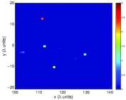
Figure 3: Images reconstructed by solving (11) and (12) when single illumination is used. From left to right, there is $0\%$, $10\%$, and $20\%$ additive noise in the data.

When multiple illuminations are used we expect a general improvement in the images. Figure 4 shows the results of the MMV algorithm when $5$ random illuminations are used. By multiple random illuminations we mean a set of illuminations coming, each one, from only one of the transducers on the array at a time, i.e., $\widehat{f}_{p}=1$ and $\widehat{f}_{q}=0$ for $q\neq p$, with $p$ chosen randomly at a time. The set of illuminations used in each image of Figure 4 is different. The data contain $10\%$ (left), $20\%$ (middle) and $50\%$ (right) of additive noise. We observe that the images obtained with multiple illuminations are more stable with respect to additive noise. However, we still see some missing scatterers in the right image ($50\%$ of noise), and therefore, for this particular set of randomly chosen illuminations, imaging is still affected by screening effect.

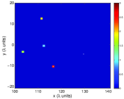
Figure 4: Images reconstructed by solving (22) when $5$ random illuminations are used. From left to right, there is $10\%$, $20\%$, and $50\%$ noise in the data.

Figure 4 shows the necessity of using “good” illuminations that maximize the information content of the data, especially when the signal-to-noise ratio (SNR) is low. Figure 5 displays the images obtained with $1$ (left), $2$ (middle), and $3$ (right), optimal illuminations associated to the singular vectors $\mbox{\boldmath{$\widehat{f}$}}^{j}=\widehat{V}_{\cdot j}$, with $j=1,2,3$. It is remarkable that only a few of them ($2$ or $3$) are enough to obtain very good images, even with $50\%$ of additive noise in the data.

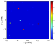
Figure 5: Images reconstructed by solving (22) when optimal illuminations are used. From left to right, the images are reconstructed by using $1$, $2$, and $3$ top singular vectors as illumination vectors. There is $50\%$ noise in the data.

4 Single scattering as a special case: The hybrid-$\ell_{1}$ method

In situations where the scatterers are weak and/or are very far apart, the incident wave undergoes only one scattering event before coming back to the array. In these cases, the inverse of the Foldy-Lax matrix $\mathbf{Z}^{-1}(\mbox{\boldmath$\rho$})$ in (6) becomes the identity matrix, and the array response matrix under the so called Born approximation becomes

$$\widehat{\mbox{\boldmath$\Pi$}}=\mbox{\boldmath{${\cal G}$}}_{0}\mathrm{diag}(\mbox{\boldmath$\rho$}_{0})\mbox{\boldmath{${\cal G}$}}_{0}^{T}\,.$$

Then, the data received on the array when an illumination vector $\widehat{f}$ probes the medium is given by $\mbox{\boldmath{$b$}}=\widehat{\mbox{\boldmath$\Pi$}}\mbox{\boldmath{$\widehat{f}$}}$. Similar to (8), we can model the data $b$ as applying the operator $\mbox{\boldmath{${\cal A}$}}_{\widehat{f}}$ to the unknown reflectivity vector $\mbox{\boldmath$\rho$}_{0}$. Because multiple scattering is negligible, $\widehat{g}_{\widehat{f}}(\mbox{\boldmath{$y$}}_{j})=\mbox{\boldmath{$\widehat{g}$}}^{T}_{0}(\mbox{\boldmath{$y$}}_{j})\mbox{\boldmath{$\widehat{f}$}}$ in (7), and thus, (8) is now linear in $\mbox{\boldmath$\rho$}_{0}$, which we denote as $\mbox{\boldmath{${\cal A}$}}_{0\widehat{f}}$. Therefore, array imaging of localized scatterers in homogeneous media when multiple scattering is negligible amounts to solving the linear optimization problem

$$\min\|\mbox{\boldmath$\rho$}\|_{\ell_{1}}\qquad\text{s.t.}\qquad\mbox{\boldmath{${\cal A}$}}_{0\widehat{f}}\mbox{\boldmath$\rho$}=\mbox{\boldmath{$b$}}.$$ (24)

In (24) we assume that the data is noiseless. If the data contains noise, we solve

$$\min\|\mbox{\boldmath$\rho$}\|_{\ell_{1}}\qquad\text{s.t.}\qquad\|\mbox{\boldmath{${\cal A}$}}_{0\widehat{f}}\mbox{\boldmath$\rho$}-\mbox{\boldmath{$b$}}\|_{\ell_{2}}<\delta\,.$$ (25)

Because of the linearity of the equations, a single-step process is sufficient to recover both the locations and reflectivities of the scatterers from (24) or (25). Moreover, when multiple scattering is negligible, there is no screening effect, and hence, solving the set of equations generated from a single illumination alone can produce reliable images. Note that Theorems 3.1 and 3.4 can be applied to problems (24) and (25) as well.

Similarly to the case where multiple scattering was important, we can use multiple illuminations and the MMV approach to find the reflectivity vector $\mbox{\boldmath$\rho$}_{0}$. Furthermore, imaging using optimal illuminations has a simpler form and weaker requirements on the imaging configuration when multiple scattering is negligible. Indeed, assume that the data is noiseless, and let the SVD of array response matrix be $\widehat{\mbox{\boldmath$\Pi$}}=\mbox{\boldmath{$\widehat{U}$}}\mbox{\boldmath{$\Sigma$}}\mbox{\boldmath{$\widehat{V}$}}^{\ast}$, with $M$ singular values $\{\sigma_{j}\}_{j=1}^{M}$ greater than $0$. Following the MMV formulation in §3.2, we have $\mbox{\boldmath{$b$}}^{j}=\widehat{\mbox{\boldmath$\Pi$}}\widehat{V}_{\cdot j}=\sigma_{j}\widehat{U}_{\cdot j}$ for $j=1,\ldots,M$. On the other hand, $\mbox{\boldmath{$b$}}^{j}={\cal A}_{0\widehat{V}_{\cdot j}}\mbox{\boldmath$\rho$}_{0}=\mbox{\boldmath{${\cal G}$}}_{0}\mbox{\boldmath$\gamma$}_{0}^{j}$, where $\mbox{\boldmath$\gamma$}_{0}^{j}=\mathrm{diag}(\widehat{g}_{\widehat{V}_{\cdot j}}(\mbox{\boldmath{$y$}}_{k}))\mbox{\boldmath$\rho$}_{0}$ is linear in $\mbox{\boldmath$\rho$}_{0}$, which is the major difference from (9). Now consider (23) with $\mbox{\boldmath{$\widetilde{{\cal E}}$}}=\mbox{\boldmath{$0$}}$ for symplicity, and project $\mbox{\boldmath{$B$}}_{opt}$ onto the space spanned by the top left singular vectors corresponding to the significant singular values. Denoting $\mbox{\boldmath{$\mathcal{U}$}}=[\widehat{U}_{\cdot 1},\ldots,\widehat{U}_{\cdot M}]$ and $\mbox{\boldmath{${X}$}}_{V}=[\mbox{\boldmath$\gamma$}^{1},\ldots,\mbox{\boldmath$\gamma$}^{M}]$, we get

$$\mbox{\boldmath{$\mathcal{U}$}}^{\ast}\mbox{\boldmath{${\cal G}$}}_{0}\mbox{\boldmath{${X}$}}_{V} = \left[\begin{array}[]{cccc}\widehat{U}_{\cdot 1}^{\ast}\mbox{\boldmath{${\cal G}$}}_{0}\mbox{\boldmath$\gamma$}^{1}&\widehat{U}_{\cdot 1}^{\ast}\mbox{\boldmath{${\cal G}$}}_{0}\mbox{\boldmath$\gamma$}^{2}&\cdots&\widehat{U}_{\cdot 1}^{\ast}\mbox{\boldmath{${\cal G}$}}_{0}\mbox{\boldmath$\gamma$}^{M}\\ \widehat{U}_{\cdot 2}^{\ast}\mbox{\boldmath{${\cal G}$}}_{0}\mbox{\boldmath$\gamma$}^{1}&\widehat{U}_{\cdot 2}^{\ast}\mbox{\boldmath{${\cal G}$}}_{0}\mbox{\boldmath$\gamma$}^{2}&\cdots&\widehat{U}_{\cdot 2}^{\ast}\mbox{\boldmath{${\cal G}$}}_{0}\mbox{\boldmath$\gamma$}^{M}\\ \vdots&\vdots&\vdots&\vdots\\ \widehat{U}_{\cdot M}^{\ast}\mbox{\boldmath{${\cal G}$}}_{0}\mbox{\boldmath$\gamma$}^{1}&\widehat{U}_{\cdot M}^{\ast}\mbox{\boldmath{${\cal G}$}}_{0}\mbox{\boldmath$\gamma$}^{2}&\cdots&\widehat{U}_{\cdot M}^{\ast}\mbox{\boldmath{${\cal G}$}}_{0}\mbox{\boldmath$\gamma$}^{M}\end{array}\right]$$ (30)

$$= \mbox{\boldmath{$\mathcal{U}$}}^{\ast}\mbox{\boldmath{$B$}}_{opt}=\mathrm{diag}(\sigma_{1},\ldots,\sigma_{M}).$$ (31)

In (30), there are $M$ unknowns $\mbox{\boldmath$\gamma$}^{1},\ldots,\mbox{\boldmath$\gamma$}^{M}$, and $M^{2}$ equations. However, when multiple scattering is negligible we can associate a nonzero singular value to each scatterer and the corresponding singular vector is given by

$$\widehat{U}_{\cdot j}=\overline{\widehat{V}_{\cdot j}}\propto\frac{\mbox{\boldmath{$\widehat{g}$}}_{0}(\mbox{\boldmath{$y$}}_{j})}{\|\mbox{\boldmath{$\widehat{g}$}}_{0}(\mbox{\boldmath{$y$}}_{j})\|_{\ell_{2}}},\qquad j=1,\ldots,M,$$ (32)

up to an arbitrary complex constant of modulus $1$. Therefore, the rank-$1$ matrices $\widehat{V}_{\cdot j}\widehat{U}_{\cdot i}^{\ast}$ have a (non-trivial) eigenvalue different from zero only when $i=j$. That is, only the diagonal blocks of the matrix $\mbox{\boldmath{$\mathcal{U}$}}^{\ast}\mbox{\boldmath{${\cal G}$}}_{0}\mbox{\boldmath{${X}$}}_{V}$ contribute in (30), and hence, we can simplify (30) further as a set of $M$ equations. Using (32) and

$$\widehat{U}_{\cdot i}^{\ast}\mbox{\boldmath{${\cal G}$}}_{0}\mbox{\boldmath$\gamma$}^{j}=\sum_{k=1}^{N}\big{(}\widehat{U}_{\cdot i}^{\ast}\mbox{\boldmath{$\widehat{g}$}}_{0}(\mbox{\boldmath{$y$}}_{k})\big{)}\big{(}\mbox{\boldmath{$\widehat{g}$}}_{0}(\mbox{\boldmath{$y$}}_{k})^{\ast}\widehat{V}_{\cdot j}\big{)}\rho_{0k}=\sum_{k=1}^{N}\mbox{\boldmath{$\widehat{g}$}}_{0}^{\ast}(\mbox{\boldmath{$y$}}_{k})\big{(}\widehat{V}_{\cdot j}\widehat{U}_{\cdot i}^{\ast}\big{)}\mbox{\boldmath{$\widehat{g}$}}_{0}(\mbox{\boldmath{$y$}}_{k})\rho_{0k}\,,$$

we can write (30) as a set of $M$ equations linear in $\mbox{\boldmath$\rho$}_{0}$ such that

$$\mbox{\boldmath{${\cal B}$}}\mbox{\boldmath$\rho$}_{0}=[\sigma_{1},\ldots,\sigma_{M}]^{T}\,,$$ (33)

where

$$\mbox{\boldmath{${\cal B}$}}=\left[\begin{array}[]{ccc}\overline{\mbox{\boldmath{$\widehat{g}$}}_{0}^{\ast}(\mbox{\boldmath{$y$}}_{1})\widehat{U}_{\cdot 1}}\mbox{\boldmath{$\widehat{g}$}}_{0}^{T}(\mbox{\boldmath{$y$}}_{1})\widehat{V}_{\cdot 1}&\cdots&\overline{\mbox{\boldmath{$\widehat{g}$}}_{0}^{\ast}(\mbox{\boldmath{$y$}}_{K})\widehat{U}_{\cdot 1}}\mbox{\boldmath{$\widehat{g}$}}_{0}^{T}(\mbox{\boldmath{$y$}}_{K})\widehat{V}_{\cdot 1}\\ \cdots&\ddots&\cdots\\ \overline{\mbox{\boldmath{$\widehat{g}$}}_{0}^{\ast}(\mbox{\boldmath{$y$}}_{1})\widehat{U}_{\cdot M}}\mbox{\boldmath{$\widehat{g}$}}_{0}^{T}(\mbox{\boldmath{$y$}}_{1})\widehat{V}_{\cdot M}&\cdots&\overline{\mbox{\boldmath{$\widehat{g}$}}_{0}^{\ast}(\mbox{\boldmath{$y$}}_{K})\widehat{U}_{\cdot M}}\mbox{\boldmath{$\widehat{g}$}}_{0}^{T}(\mbox{\boldmath{$y$}}_{K})\widehat{V}_{\cdot M}\\ \end{array}\right].$$

Therefore, the hybrid-$\ell_{1}$ method is to solve for $\mbox{\boldmath$\rho$}_{0}$ from the SMV problem

$$\min\|\mbox{\boldmath$\rho$}\|_{\ell_{1}}\qquad\text{s.t.}\qquad\mbox{\boldmath{${\cal B}$}}\mbox{\boldmath$\rho$}=[\sigma_{1},\ldots,\sigma_{M}]^{T}\,.$$ (34)

The advantage of hybrid-$\ell_{1}$ method compared to the MMV formulation is its simpler form and lower dimensionality. Moreover, the hybrid $\ell_{1}$ method guarantees exact recovery, the sufficient condition for which also implies that it can form images with higher resolution (see [16] for details).

Theorem 4.1.

Assume that the scatterers are far part such that (32) is satisfied. Let $E$ be the submatrix of ${\cal B}$ formed by normalized columns corresponding to the scatterers’ location and $S$ be the submatrix formed by the remaining normalized columns of ${\cal B}$. If $\|\mbox{\boldmath{$S$}}\|_{1\rightarrow 1}<1-\|\mbox{\boldmath{$E$}}-\mbox{\boldmath{$I$}}\|_{1\rightarrow 1}$, where $\|\cdot\|_{1\rightarrow 1}$ is the matrix $1$-norm induced by the vector $\ell_{1}$ norm, and $I$ is the identity matrix, then $\mbox{\boldmath$\rho$}_{0}$ is the unique solution to (34).

4.1 Numerical experiments

Now we present the results of a numerical experiment that shows the performance of the hybrid-$\ell_{1}$ method compared to those obtained with KM and MUSIC. We consider the same imaging set-up as in subsection 3.4. KM is a simple and robust imaging method (with respect to additive noise) which propagates the imaging data received on the array back to the medium. Under the setup of imaging in §2, the KM imaging functional can be written as

$$\mbox{\boldmath$\rho$}_{KM}=\mbox{\boldmath{${\cal A}$}}_{0\widehat{f}}^{\ast}\mbox{\boldmath{$b$}}.$$ (35)

MUSIC, on the other hand, is a subspace projection algorithm that uses the SVD of the array response matrix. The idea of MUSIC is to project the reference illumination vectors $\mbox{\boldmath{$\widehat{g}$}}_{0}(\mbox{\boldmath{$y$}}_{j})$, $j=1,\dots,M$, onto the noise space using the projection operator

$$\mathcal{P}\mbox{\boldmath{$\widehat{g}$}}_{0}(\mbox{\boldmath{$y$}})=\sum_{j=1}^{M}(\widehat{U}^{\ast}_{\cdot j}\mbox{\boldmath{$\widehat{g}$}}_{0}(\mbox{\boldmath{$y$}}))\widehat{U}_{\cdot j}-\mbox{\boldmath{$\widehat{g}$}}_{0}(\mbox{\boldmath{$y$}}).$$ (36)

Then, according to (32), the normalized functional

$$\mathcal{I}_{MUSIC}(\mbox{\boldmath{$y$}}_{k})=\frac{\min_{1\leq j\leq K}\|\mathcal{P}\mbox{\boldmath{$\widehat{g}$}}_{0}(\mbox{\boldmath{$y$}}_{j})\|_{\ell_{2}}}{\|\mathcal{P}\mbox{\boldmath{$\widehat{g}$}}_{0}(\mbox{\boldmath{$y$}}_{k})\|_{\ell_{2}}},\quad k=1,\ldots,K,$$ (37)

will peak at the search points $\mbox{\boldmath{$y$}}_{k}$ only at locations where there is a scatterer. Imaging with MUSIC (37) only locates of the scatterer’s positions. Their reflectivities are usually obtained using a separate procedure after the locations are known.

Figure 6 shows the simulation results with $100\%$ of additive noise in the data. From left to right, we display the images obatined with KM, MUSIC and the hybrid-$\ell_{1}$ method. In the simulations for MUSIC and hybrid-$\ell_{1}$ we assume that the top $5$ singular vectors have been obtained. In the simulations for KM we use $5$ random illuminations. It is apparent that the image created by the hybrid-$\ell_{1}$ method is better than the other two. The hybrid-$\ell_{1}$ method forms a clear image with perfect recovery of the location of the scatterers, and accurate estimates of their reflectivities. The robustness of the hybrid-$\ell_{1}$ method relies on the selection of the top singular values so that the noise in the subspace formed by singular vectors associated with small singular values is filtered out.

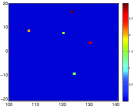
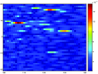
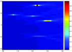
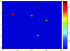
Figure 6: Images obtained using KM (left), MUSIC (middle), and hybrid-$\ell_{1}$ (right) with $100\%$ noise in data. We use $5$ illuminations in KM.

5 Active array imaging in random media

Many natural media vary randomly in space, and therefore, waves propagating in these media also fluctuate in space. Thus the data collected on the array inherit the uncertainty of the fluctuations of the medium resulting in wave distortion. Because wave distortion effects induced by the inhomogeneities are very different from additive uncorrelated noise, imaging through random media is very different from that in homogeneous media. For example, the images obtained by Kirchhoff migration become noisy and change unpredictably with the detailed features of the medium, and thus, are useless. In this section, we use a simple random phase model to analyze the performance of the hybrid-$\ell_{1}$ and MUSIC methods in random media. Both methods use the SVD of the response matrix. The random phase model distorts the wavefronts but keeps the amplitude of the waves unchanged and is valid in the regime of geometrical optics.

5.1 Random phase model

In random media, the Green’s function that characterizes the wave propagation from $x$ to $y$ is given by the wave equation

$$\Delta\widehat{G}(\mbox{\boldmath{$x$}},\mbox{\boldmath{$y$}})+\kappa^{2}n^{2}(\mbox{\boldmath{$x$}})\widehat{G}(\mbox{\boldmath{$x$}},\mbox{\boldmath{$y$}})=\delta(\mbox{\boldmath{$x$}}-\mbox{\boldmath{$y$}}),$$ (38)

where $n(\mbox{\boldmath{$x$}})=\frac{c_{0}}{c(\mbox{\boldmath{$x$}})}$ is the random index of refraction of the medium with local wave speed $c(\mbox{\boldmath{$x$}})$. In a homogeneous medium, we have $c(\mbox{\boldmath{$x$}})\equiv c_{0}$ for any location $x$, and hence, $\widehat{G}_{0}(\mbox{\boldmath{$x$}},\mbox{\boldmath{$y$}})$ defined in (2) is the solution to (38). In random media, however, the wave speed $c(\mbox{\boldmath{$x$}})$ depends on the position $x$. In this paper, we consider random fluctuations of the wave speed satisfying the model

$$\frac{1}{c^{2}(\mbox{\boldmath{$x$}})}=\frac{1}{c_{0}^{2}}\bigg{(}1+\sigma\mu(\frac{\mbox{\boldmath{$x$}}}{l})\bigg{)}\,,$$ (39)

where $l$ is the correlation length of the medium, $\sigma$ determines the strength of the flucutation around the constant speed $c_{0}$, and $\mu(\cdot)$ is a stationary random process with zero mean and normalized autocorrelation function $R(|\mbox{\boldmath{$x$}}-\mbox{\boldmath{$x$}}^{\prime}|)=\mathbb{E}(\mu(\mbox{\boldmath{$x$}})\mu(\mbox{\boldmath{$x$}}^{\prime}))$, so $R(0)=1$. Here, we only consider weak fluctuations such that $\sigma\ll 1$.

When the index of refraction $n(\mbox{\boldmath{$x$}})$ is random, there is no analytic solution to (38), and hence, numerical schemes are often used to obtained an approximated numerical solution. This can be time consuming, especially for large distances $L$. Instead, the random phase model provides an analytical approximation for the Green’s function between two points at a distance of order $L\gg l\gg\lambda$ from each other, given by

$$\widehat{G}(\mbox{\boldmath{$x$}},\mbox{\boldmath{$y$}})=\widehat{G}_{0}(\mbox{\boldmath{$x$}},\mbox{\boldmath{$y$}})\exp{\left[\mathrm{i}\sigma\kappa|\mbox{\boldmath{$x$}}-\mbox{\boldmath{$y$}}|\int_{0}^{1}\mu(\frac{\mbox{\boldmath{$x$}}}{l}+\frac{s}{l}(\mbox{\boldmath{$y$}}-\mbox{\boldmath{$x$}}))\,\mathrm{d}s\right]}.$$ (40)

This approximation is valid when (i) the wavelength $\lambda$ is much smaller than the correlation length $l$ so the geometric optics approximation holds, (ii) the correlation length $l$ is much smaller than the propagation distance $L$ so the statistics of the phase is Gaussian, and (iii) the strength of the fluctuation $\sigma$ is small so the amplitude of the wave is kept unchanged, but large enough to ensure that the perturbations of the phases are not negligible. The last condition holds when $\frac{\sigma^{2}L^{3}}{l^{3}}\ll\frac{\lambda^{2}}{\sigma^{2}lL}\leq 1$ (for details, see [38, 35, 9]). Note that although we take weak fluctuations, the distortion of the wavefronts by the inhomogeneities of the medium is observable because the wave travels long distances.

Comparing (40) to the homogeneous Green’s function (2) we see that, in this regime, only the phase is perturbed by the random medium and the magnitude remains unchanged. The following result shows that the second order moment of (40) is close to the expected value.

Proposition 5.1.

Assume that the autocorrelation function $R\in\mathbb{L}_{2}(\mathbb{R}_{+})$ is differentiable and its derivative $\dot{R}$ satisfies $\frac{\dot{R}(t)}{t}\in\mathbb{L}(\mathbb{R}_{+})$ with exponential decay. Let $\mbox{\boldmath{$y$}}_{1}$ and $\mbox{\boldmath{$y$}}_{2}$ be two points on the same plane at a distance $L$ from point $x$, such that $\lambda\ll|\mbox{\boldmath{$y$}}_{1}-\mbox{\boldmath{$y$}}_{2}|\ll L$. Then, for the Green’s function (40) we have

$$\mathbb{E}\bigg{(}\widehat{G}(\mbox{\boldmath{$x$}},\mbox{\boldmath{$y$}}_{1})\overline{\widehat{G}(\mbox{\boldmath{$x$}},\mbox{\boldmath{$y$}}_{2})}\bigg{)}\approx\widehat{G}_{0}(\mbox{\boldmath{$x$}},\mbox{\boldmath{$y$}}_{1})\overline{\widehat{G}_{0}(\mbox{\boldmath{$x$}},\mbox{\boldmath{$y$}}_{2})}\mathrm{e}^{-\frac{\kappa^{2}a_{e}^{2}}{2L^{2}}|\mbox{\boldmath{$y$}}_{1}-\mbox{\boldmath{$y$}}_{2}|^{2}},$$ (41)

with

$$a_{e}=\sigma L\left(-1-\frac{2L}{3l}\int_{0}^{\infty}\frac{\dot{R}(t)}{t}\,\mathrm{d}t\right)^{\frac{1}{2}}.$$ (42)

According to Proposition 5.1, the back-propagated signal in random media is equal to that in a homogeneous medium times a Gaussian factor with variance $\frac{L^{2}}{\kappa^{2}a_{e}^{2}}$. The length $a_{e}$ is an intrinsic property of the random media. It depends on the propagation distance $L$ and the statistics of the random fluctuations of the medium. According to (41), as $a_{e}$ increases, the refocused spot size for time reversal in random media is tighter. Using the moment estimate (41), we immediately have the following variance estimate.

Corollary 5.2.

Under the same conditions given in Proposition 5.1, we have for (40)

$$\mathbb{E}\left|\widehat{G}(\mbox{\boldmath{$x$}},\mbox{\boldmath{$y$}}_{1})\overline{\widehat{G}(\mbox{\boldmath{$x$}},\mbox{\boldmath{$y$}}_{2})}-\mathbb{E}\left(\widehat{G}(\mbox{\boldmath{$x$}},\mbox{\boldmath{$y$}}_{1})\overline{\widehat{G}(\mbox{\boldmath{$x$}},\mbox{\boldmath{$y$}}_{2})}\right)\right|^{2}\approx\frac{1-\mathrm{e}^{-\frac{\kappa^{2}a_{e}^{2}}{L^{2}}|\mbox{\boldmath{$y$}}_{1}-\mbox{\boldmath{$y$}}_{2}|^{2}}}{16\pi^{2}|\mbox{\boldmath{$x$}}-\mbox{\boldmath{$y$}}_{1}|^{2}|\mbox{\boldmath{$x$}}-\mbox{\boldmath{$y$}}_{2}|^{2}}.$$ (43)

This property of the Green’s function (40) is generally referred to as self-averaging, which means that a time-reversed, back-propagated signal in a random medium refocuses near the source independently of the particular realization of the random medium. Self-averaging properties of back-propagated signals in random media have been shown under broad-band settings, see for example [25, 5, 2, 33, 34], but are not true, in general, for narrow-band signals. Corollary 5.2 states that the Green’s function corresponding to the phase random model (40) exhibits the same properties, even for narrow-band pulses.

The next result states that a single realization of a back-propagated signal via the Green’s function vector $\mbox{\boldmath{$\widehat{g}$}}(\mbox{\boldmath{$y$}})$ (1) is stable when the aperture of the imaging array becomes infinity, in the sense that its value is close to the back-propagated signal averaged over multiple realizations.

Proposition 5.3.

For a large aperture size $a$, the signal sent from $\mbox{\boldmath{$y$}}_{1}$, recorded at the array, and back-propagated at $\mbox{\boldmath{$y$}}_{2}$ is statistically stable for (40) in the sense that

$$\frac{\mathbb{E}|\mbox{\boldmath{$\widehat{g}$}}^{\ast}(\mbox{\boldmath{$y$}}_{1})\mbox{\boldmath{$\widehat{g}$}}(\mbox{\boldmath{$y$}}_{2})-\mathbb{E}(\mbox{\boldmath{$\widehat{g}$}}^{\ast}(\mbox{\boldmath{$y$}}_{1})\mbox{\boldmath{$\widehat{g}$}}(\mbox{\boldmath{$y$}}_{2}))|^{2}}{\mathbb{E}\|\mbox{\boldmath{$\widehat{g}$}}(\mbox{\boldmath{$y$}}_{1})\|^{2}\mathbb{E}\|\mbox{\boldmath{$\widehat{g}$}}(\mbox{\boldmath{$y$}}_{2})\|^{2}}\rightarrow 0,\qquad a\rightarrow\infty.$$ (44)

Furthermore, as shown in Appendix B, the decay rate of (44) is bounded by

$$\left(1-\mathrm{e}^{-\frac{\kappa^{2}}{L^{2}}|\mbox{\boldmath{$y$}}_{1}-\mbox{\boldmath{$y$}}_{2}|^{2}a_{e}^{2}}\right)\left(\frac{l^{2}}{L^{2}\log\left(1+\frac{a^{2}}{4L^{2}}\right)}\right)$$ (45)

for any aperture size $a$. Thus, for short distances so $L$ is of order $a$, the decay rate is only logarithmic in $a$. However, when the distance is large such that $L\gg a$ (e.g. the remote sensing regime), we can use a linear approximation on the logarithm function and obtain, up to a constant, the approximated decay rate

$$\left(1-\mathrm{e}^{-\frac{\kappa^{2}}{L^{2}}|\mbox{\boldmath{$y$}}_{1}-\mbox{\boldmath{$y$}}_{2}|^{2}a_{e}^{2}}\right)\left(\frac{l}{a}\right)^{2},$$ (46)

which implies a quadratic decay rate in $a$. Such quadratic decay rate in $a$ can also be justified by using the paraxial approximation when $L\gg a$. As it is noted in Remark B.2, the decay rate in the paraxial approximation is given by (66), so the bound in (46) coincides with the paraxial approximation up to oscillations caused by the $\mathrm{sinc}$ function.

We emphasize that, although (45) indicates little improvement in the refocused spot size when the physical aperture of the array $a$ is large, Proposition 5.3 implies that large arrays stabilize refocusing of narrow-band pulses in random media. The fact that large arrays improve the quality of imaging in cluttered media has been recognized for long time in radar and seismic imaging. The theoretical results obtained here using the random phase model support this empirical observation.

Next, we give a result that is essential for the performance of hybrid-$\ell_{1}$ and MUSIC methods in random media. When imaging in random media, the Green’s function vector $\mbox{\boldmath{$\widehat{g}$}}(\mbox{\boldmath{$y$}})$ is random and not known. The best we can do is to use the deterministic Green’s function vector $\mbox{\boldmath{$\widehat{g}$}}_{0}(\mbox{\boldmath{$y$}})$ which is, in general, quite different from the random one. Furthermore, replacement of $\mbox{\boldmath{$\widehat{g}$}}(\mbox{\boldmath{$y$}})$ by $\mbox{\boldmath{$\widehat{g}$}}_{0}(\mbox{\boldmath{$y$}})$ might give good results for some realizations of the random medium but not for others. The next result tells us that a single realization of a narrow-band backpropagated signal $\mbox{\boldmath{$\widehat{g}$}}_{0}^{\ast}(\mbox{\boldmath{$y$}}_{1})\mbox{\boldmath{$\widehat{g}$}}(\mbox{\boldmath{$y$}}_{2})$, with the Green’s function corresponding to the phase random model, is stable as the aperture of the array becomes infinity, which means that its value is close to the back-propagated signal averaged over multiple realizations.

Proposition 5.4.

Let $\mbox{\boldmath{$y$}}_{1}$ and $\mbox{\boldmath{$y$}}_{2}$ be two points satisfying $\lambda\ll|\mbox{\boldmath{$y$}}_{1}-\mbox{\boldmath{$y$}}_{2}|\ll L$. Then, for the Green’s function (40), we asymptotically have

$$\mbox{\boldmath{$\widehat{g}$}}^{\ast}(\mbox{\boldmath{$y$}}_{1})\mbox{\boldmath{$\widehat{g}$}}(\mbox{\boldmath{$y$}}_{2})\rightarrow 0\,,\qquad a\rightarrow\infty,$$ (47)

and for the mixed inner products

$$\mbox{\boldmath{$\widehat{g}$}}_{0}^{\ast}(\mbox{\boldmath{$y$}}_{1})\mbox{\boldmath{$\widehat{g}$}}(\mbox{\boldmath{$y$}}_{2})\rightarrow 0\,,\qquad a\rightarrow\infty\,,$$ (48)

where the limit is under probability measure $\mathbb{P}$ induced by $\mu(\cdot)$. Moreover, the mixed inner product is also statistically stable in the sense that

$$\frac{\mathbb{E}\left|\mbox{\boldmath{$\widehat{g}$}}_{0}^{\ast}(\mbox{\boldmath{$y$}}_{1})\mbox{\boldmath{$\widehat{g}$}}(\mbox{\boldmath{$y$}}_{2})-\mathbb{E}(\mbox{\boldmath{$\widehat{g}$}}_{0}^{\ast}(\mbox{\boldmath{$y$}}_{1})\mbox{\boldmath{$\widehat{g}$}}(\mbox{\boldmath{$y$}}_{2}))\right|^{2}}{\|\mbox{\boldmath{$\widehat{g}$}}_{0}(\mbox{\boldmath{$y$}}_{1})\|^{2}\mathbb{E}\|\mbox{\boldmath{$\widehat{g}$}}(\mbox{\boldmath{$y$}}_{2})\|^{2}}\rightarrow 0,\quad a\rightarrow\infty.$$ (49)

Proposition 5.4 implies that imaging in random media, i.e., a narrow-band pulse $\mbox{\boldmath{$\widehat{g}$}}(\mbox{\boldmath{$y$}}_{2})$ back-propagated via $\mbox{\boldmath{$\widehat{g}$}}_{0}(\mbox{\boldmath{$y$}}_{1})$ in the medium, is statistically stable for large arrays, and the pulse heading to the point $\mbox{\boldmath{$y$}}_{1}$ will focus around the correct location $\mbox{\boldmath{$y$}}_{2}$.

5.2 The hybrid-$\ell_{1}$ method

Assume that multiple scattering between the scatterers is negligible, and wave distortion is well described by the random phase model (40). Then, the response matrix has the form

$$\mbox{\boldmath{$\widehat{P}$}}=\sum_{j=1}^{M}\alpha_{j}\mbox{\boldmath{$\widehat{g}$}}(\mbox{\boldmath{$y$}}_{n_{j}})\mbox{\boldmath{$\widehat{g}$}}^{T}(\mbox{\boldmath{$y$}}_{n_{j}})\,,$$ (50)

with random Green’s function vectors $\mbox{\boldmath{$\widehat{g}$}}(\mbox{\boldmath{$y$}})=[\widehat{G}(\mbox{\boldmath{$x$}}_{1},\mbox{\boldmath{$y$}}),\ldots,\widehat{G}(\mbox{\boldmath{$x$}}_{N},\mbox{\boldmath{$y$}})]^{T}$, where $\widehat{G}(\mbox{\boldmath{$x$}},\mbox{\boldmath{$y$}})$ is given by (40). Because multiple scattering is not important, the transformation $\mbox{\boldmath{${\cal A}$}}_{\widehat{f}}\mbox{\boldmath$\rho$}=\mbox{\boldmath{$b$}}$ that relates the reflectivity vector $\mbox{\boldmath$\rho$}_{0}$ with the data measured at the array $b$ is linear. However, when the medium contains random inhomogeneities, this linear transformation is random because the column vectors of the operator $\mbox{\boldmath{${\cal A}$}}_{\widehat{f}}$ are random functions. Therefore, to solve for the reflectivity vector $\mbox{\boldmath$\rho$}_{0}$, we have to approximate the unknown Green’s function vectors $\mbox{\boldmath{$\widehat{g}$}}(\mbox{\boldmath{$y$}})$ by the ones for a homogeneous medium, after which, $\mbox{\boldmath{${\cal A}$}}_{\widehat{f}}$ becomes the linear operator $\mbox{\boldmath{${\cal A}$}}_{0\widehat{f}}$ given in §4. The substitution of $\mbox{\boldmath{$\widehat{g}$}}(\mbox{\boldmath{$y$}})$ by $\mbox{\boldmath{$\widehat{g}$}}_{0}(\mbox{\boldmath{$y$}})$ introduces a discrepancy between model and data, and thus, we must solve the $\ell_{1}$ minimization problem (25) with an inequality constraint when data from a single illumination is available. We note that to estimate the error bound of such discrepancy is nontrivial due to the existing correlation in the measurement noise in random media.

According to Proposition 5.4, when the scatterers are far apart, the random Green’s function vectors $\mbox{\boldmath{$\widehat{g}$}}(\mbox{\boldmath{$y$}}_{n_{j}})$, $j=1,\dots,M$, are approximately orthogonal in probability as the size of the imaging array becomes large. In this case, we can associate to each of the $M$ scatterers a nonzero singular value $\sigma_{j}=\alpha_{j}\|\mbox{\boldmath{$\widehat{g}$}}(\mbox{\boldmath{$y$}}_{n_{j}})\|_{\ell_{2}}^{2}$ with singular vectors

$$\widehat{U}_{\cdot j}=\frac{\mbox{\boldmath{$\widehat{g}$}}(\mbox{\boldmath{$y$}}_{n_{j}})}{\|\mbox{\boldmath{$\widehat{g}$}}(\mbox{\boldmath{$y$}}_{n_{j}})\|_{\ell_{2}}},\quad\widehat{V}_{\cdot j}=\overline{\frac{\mbox{\boldmath{$\widehat{g}$}}(\mbox{\boldmath{$y$}}_{n_{j}})}{\|\mbox{\boldmath{$\widehat{g}$}}(\mbox{\boldmath{$y$}}_{n_{j}})\|_{\ell_{2}}}}\,,\qquad j=1,\dots,M.$$ (51)

If the full array response matrix $\widehat{P}$ (or its SVD) is available, we can use the hybrid-$\ell_{1}$ as follows. We use the right singular vectors of $\widehat{P}$ as the illumination vectors, and we project the data to the space spanned by the left singular vectors in the same way as shown in §4. Thus, we form the same hybrid-$\ell_{1}$ optimization given in (34) and there is no need to estimate the error bound of the discrepancy between model and data. Recall that $(ij)^{\mathrm{th}}$ entry of the hybrid-$\ell_{1}$ matrix ${\cal B}$ is related to the singular vectors in the form of $\overline{\mbox{\boldmath{$\widehat{g}$}}_{0}^{\ast}(\mbox{\boldmath{$y$}}_{j})\widehat{U}_{\cdot i}}\mbox{\boldmath{$\widehat{g}$}}_{0}^{T}(\mbox{\boldmath{$y$}}_{j})\widehat{V}_{\cdot i}$, and the singular vectors of the response matrix $\widehat{P}$ are related to the random Green’s function vectors as in (51). Hence, each entry is the mixed inner product (48) between $\mbox{\boldmath{$\widehat{g}$}}_{0}(\mbox{\boldmath{$y$}}_{j})$ and $\mbox{\boldmath{$\widehat{g}$}}(\mbox{\boldmath{$y$}}_{i})$.

Without loss of generality, assume that the $M$ scatterers correspond to the first $M$ columns in ${\cal B}$, i.e. $n_{j}=j$, $j=1,\ldots,M$. We can write ${\cal B}$ in the form of block matrices as $\mbox{\boldmath{${\cal B}$}}=[\mbox{\boldmath{${\cal B}$}}_{M\times M}\ \ \mbox{\boldmath{$S$}}]$, where the columns in $S$ correspond to grid points where there is no scatterers. Due to Proposition 5.4, the submatrix $\mbox{\boldmath{${\cal B}$}}_{M\times M}$ is a diagonal matrix $D$ perturbed by a matrix $E$ with $\|\mbox{\boldmath{$E$}}\|_{1\rightarrow 1}\ll 1$. The value of $\|\mbox{\boldmath{$E$}}\|_{1\rightarrow 1}$ depends on the minimal distance between any two scatterers, and is close to zero if they are well separated. Due to the incomplete phase cancellation in the mixed inner products, $D$ is composed of complex values but, as long as the scatterers are far apart, $\mbox{\boldmath{$D$}}+\mbox{\boldmath{$E$}}$ is diagonal dominated. Furthermore, because of the statistical stability of the mixed inner product (49), if $\|\mbox{\boldmath{$D$}}^{-1}\mbox{\boldmath{$S$}}\|_{1\rightarrow 1}<1-\|\mbox{\boldmath{$D$}}^{-1}\mbox{\boldmath{$E$}}\|_{1\rightarrow 1}$, (34) gives the right solution even though there exists (correlated) noise in the data caused by the random media. This saves computational time by eliminating the need for difficult error bounds testing.

5.3 MUSIC

In random media, the exact knowledge of the reference illumination $\mbox{\boldmath{$\widehat{g}$}}(\mbox{\boldmath{$y$}})$ is unknown, and therefore imaging using MUSIC amounts to approximate the unknow illumination with that in homogeneous context, i.e.

$$\mathcal{I}^{RM}_{MUSIC}(\mbox{\boldmath{$y$}}_{k})=\frac{\min_{1\leq j\leq K}\|\mathcal{P}\mbox{\boldmath{$\widehat{g}$}}_{0}(\mbox{\boldmath{$y$}}_{j})\|_{\ell_{2}}}{\|\mathcal{P}\mbox{\boldmath{$\widehat{g}$}}_{0}(\mbox{\boldmath{$y$}}_{k})\|_{\ell_{2}}},\quad k=1,\ldots,K.$$ (52)

According to (51) and (48), the proxy $\mbox{\boldmath{$\widehat{g}$}}_{0}(\mbox{\boldmath{$y$}})$ will focus around the scatterers when the imaging array is large enough. However, the image obtained by (52) will have lower resolution compared to the ideal case of (37), since the random phase in $\mbox{\boldmath{$\widehat{g}$}}(\mbox{\boldmath{$y$}})$ cannot be fully cancelled out using the homogenous Green’s function vector $\mbox{\boldmath{$\widehat{g}$}}_{0}(\mbox{\boldmath{$y$}})$.

5.4 Numerical experiments

Figure 7: Original configuration of the scatterers in a $41\times 41$ image window with grid points separated by $1$.

We now present numerical simulations in two dimensions to illustrate the performance of the MUSIC and hybrid-$\ell_{1}$ imaging methods in random media. We consider a random medium with correlation length $l=20\lambda$, and standard deviation of the fluctuations $\sigma=0.1\%$. For comparison purposes we also show images obtained by Kirchhoff migration with a single illumination sent from the central transducer of the array.

We consider a small and a large array, both consisting of $501$ transducers uniformily distributed over the aperture. The small array has an aperture of $25l$, and the large array an aperture of $100l$. Four scatterers are placed within an IW of size $41\lambda\times 41\lambda$, which is at a distance $L=50l$ from the linear array, see Figure 7. We discretize the IW using a uniform grid with points separated by one wavelength $\lambda$ (the spatial unit in all the figures is $\lambda$). The amplitudes of the reflectivities of the scatterers, $|\alpha_{j}|$, are $0.8$, $1.0$, $0.5$, and $0.7$. The phases are set randomly in each realization. We compute the array data (50) using the Green’s function given by (40). The line integral of the random field in (40) is approximated by a quadrature rule.

As a reference, we show in Figure 8 the images obtained in a homogeneous medium using KM (left column), MUSIC (center column), and hybrid-$\ell_{1}$ methods (right column) with noiseless data. The top and bottom rows show the results for the small array and the large array, respectively. As expected, the resolution of the KM images improves greatly for large arrays. On the other hand, in a homogeneous medium, MUSIC and hybrid-$\ell_{1}$ achieve an excellent resolution, even for small arrays. The images shown in Figure 8 do not change too much when the data is corrupted with up to $100\%$ of additive noise [16].

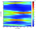
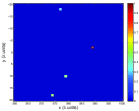
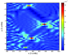
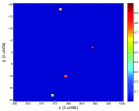
Figure 8: Top row: small array. Bottom row: large array. KM (left column), MUSIC (center column) and hybrid-$\ell_{1}$ (right column) images in homogeneous media. There is no additive noise in the data.

The situation changes when there is correlated noise in the data because the signals propagate through a random medium with a complex structure. This is illustrated in Figure 9, where we show the images produced by these imaging methods using a small array ($a=25l$). The three imaging methods show different behaviors though. Kirchhoff migration completely fails to image the scatterers, as can be seen in the top row the figure. There is not only degradation in the resolution, but also loss of stability. Observe that the images obtained with KM are significantly different from one realization to another.

The images obtained with MUSIC (middle row of Figure 9) are also blurred compared to those obtained in a homogeneous medium. Furthermore, the images change from one realization of the random medium to another and, therefore, MUSIC is also unstable if the array size is small. The hybrid-$\ell_{1}$ method also produces images that change from one realization to another (bottom row of Figure 9), but tries to keep a good resolution to provide a sparse solution. Observe that the detected scatterers dance along the cross-range direction around the true locations indicated in the figure with white dots. The images obtained with the hybrid-$\ell_{1}$ method also show some ghosts.

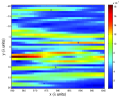
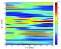
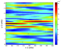
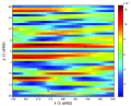
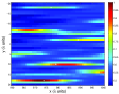
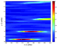
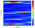
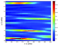
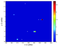
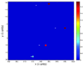
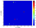
Figure 9: Small array. KM (top row) , MUSIC (center row) and hybrid-$\ell_{1}$ (bottom row) images in the same four realizations of a random medium.

These problems are overcome when the array is large ($a=100l$), see Figure 10. As expected, the resolution of the images obtained by KM and MUSIC improve a lot. However, KM still fails to image in random media as it produces clutter noise in the images from which it is hard or impossible to identify the location of the four scatterers. On the other hand, MUSIC and the hybrid-$\ell_{1}$ method are able to recover the sparse solution. We observe, though, that the performance of the hybrid-$\ell_{1}$ method is better. The locations of the four scatterers are found exactly by this method.

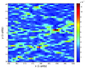
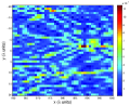
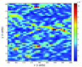
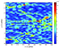
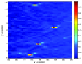
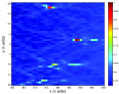
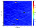
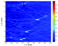
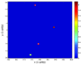
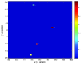
Figure 10: Large array. KM (top row) , MUSIC (center row) and hybrid-$\ell_{1}$ (bottom row) images in the same four realizations of a random medium.

6 Conclusions

We present a comprehensive study of optimization based methods applied to narrow band array imaging of localized scatterers. We have considered homogeneous and heterogeneous media. When the media is homogeneous but multiple scattering between the scatterers is important, we give a non-iterative formulation of the nonlinear inverse problem that allows us to determine the locations and reflectivities of the scatterers non-iteratively using sparsity promoting optimization. We also propose to apply optimal illuminations to improve the robustness of the imaging methods and the resolution of the images. When multiple scattering is negligible, the optimization problem becomes linear. In this case, our formulation can be reduced to a hybrid-$\ell_{1}$ method that uses the optimal illuminations and $\ell_{1}$ minimization. This method reduces the dimensionality of the problem, filters out the noise, and keeps all the essential properties of $\ell_{1}$ minimization.

When the media is random, we study the important concept of statistical stability which relates to the robustness of the imaging methods with respect to different realizations of the random media. Provided the imaging array is large enough, we show that the hybrid-$\ell_{1}$ method gives very accurate results and is statistically stable.

We illustrate the theoretical results with various numerical examples and compared the performance of the proposed optimization based methods to the widely used Kirchhoff migration and the MUSIC methods.

Appendix

Appendix A Foldy-Lax model

Multiple scattering between point-like scatterers is modeled by means of the Foldy-Lax equations [26, 27, 28]. Under this framework, the scattered wave received at transducer $\mbox{\boldmath{$x$}}_{r}$ due to a narrow band signal of angular frequency $\omega$ sent from $\mbox{\boldmath{$x$}}_{s}$ can be written as the superposition of all scattered waves from the $M$ scatterers at $\{\mbox{\boldmath{$y$}}_{n_{1}},\ldots,\mbox{\boldmath{$y$}}_{n_{M}}\}$ (see Fig. 1 (c)), so

$$\widehat{P}(\mbox{\boldmath{$x$}}_{r},\mbox{\boldmath{$x$}}_{s})=\sum_{j=1}^{M}\hat{\psi}_{j}^{s}(\mbox{\boldmath{$x$}}_{r};\mbox{\boldmath{$y$}}_{n_{1}},\ldots,\mbox{\boldmath{$y$}}_{n_{M}}).$$ (53)

Here, $\hat{\psi}_{j}^{s}(\mbox{\boldmath{$x$}}_{r};\mbox{\boldmath{$y$}}_{n_{1}},\ldots,\mbox{\boldmath{$y$}}_{n_{M}})$ represents the scattered wave observed at $\mbox{\boldmath{$x$}}_{r}$ due to the emaniting wave from the scatterer at position $\mbox{\boldmath{$y$}}_{n_{j}}$. It depends on the positions of all the scatterers and is given by

$$\hat{\psi}_{j}^{s}(\mbox{\boldmath{$x$}}_{r};\mbox{\boldmath{$y$}}_{n_{1}},\ldots,\mbox{\boldmath{$y$}}_{n_{M}})=\alpha_{j}\widehat{G}(\mbox{\boldmath{$x$}}_{r},\mbox{\boldmath{$y$}}_{n_{j}})\hat{\psi}_{j}^{e}(\mbox{\boldmath{$y$}}_{n_{1}},\ldots,\mbox{\boldmath{$y$}}_{n_{M}}),$$ (54)

where $\hat{\psi}_{j}^{e}(\mbox{\boldmath{$y$}}_{n_{1}},\ldots,\mbox{\boldmath{$y$}}_{n_{M}})$ represents the exciting field at the scatterer located at $\mbox{\boldmath{$y$}}_{n_{j}}$. Ignoring the self-interacting fields, the exciting field at $\mbox{\boldmath{$y$}}_{n_{j}}$ is equal to the sum of the incident field $\hat{\psi}^{inc}_{j}:=\hat{\psi}^{inc}(\mbox{\boldmath{$y$}}_{n_{j}},\mbox{\boldmath{$x$}}_{s})$ at $\mbox{\boldmath{$y$}}_{n_{j}}$ and the scattered fields at $\mbox{\boldmath{$y$}}_{n_{j}}$ due to all scatterers except for the one at $\mbox{\boldmath{$y$}}_{n_{j}}$. Hence, it is given by

$$\hat{\psi}_{j}^{e}(\mbox{\boldmath{$y$}}_{n_{1}},\ldots,\mbox{\boldmath{$y$}}_{n_{M}})=\hat{\psi}^{inc}(\mbox{\boldmath{$y$}}_{n_{j}},\mbox{\boldmath{$x$}}_{s})+\sum_{k\neq j}\alpha_{k}\widehat{G}(\mbox{\boldmath{$y$}}_{n_{j}},\mbox{\boldmath{$y$}}_{n_{k}})\hat{\psi}_{k}^{e}(\mbox{\boldmath{$y$}}_{n_{1}},\ldots,\mbox{\boldmath{$y$}}_{n_{M}}),$$ (55)

for $j=1,2,\ldots,M$. This is a self-consistent system of $M$ equations for the $M$ unknown exciting fields

$$\hat{\psi}_{1}^{e}:=\hat{\psi}_{1}^{e}(\mbox{\boldmath{$y$}}_{n_{1}},\ldots,\mbox{\boldmath{$y$}}_{n_{M}}),\ldots,\hat{\psi}_{M}^{e}:=\hat{\psi}_{M}^{e}(\mbox{\boldmath{$y$}}_{n_{1}},\ldots,\mbox{\boldmath{$y$}}_{n_{M}}).$$

We write (55) in matrix form as

$$\mathbf{Z}_{M}(\mbox{\boldmath{$\alpha$}})\,\mathbf{\Phi}^{e}=\mathbf{\Phi}^{inc}\,\,,$$ (56)

where $\mathbf{\Phi}^{e}=[\hat{\psi}^{e}_{1},\ldots,\hat{\psi}^{e}_{M}]^{T}$ and $\mathbf{\Phi}^{inc}=[\hat{\psi}^{inc}_{1},\ldots,\hat{\psi}^{inc}_{M}]^{T}$ are vectors whose components are the exciting and incident fields on the $M$ scatterers, respectively, and

$$\big{(}Z_{M}(\mbox{\boldmath{$\alpha$}})\big{)}_{ij}=\begin{cases}1&i=j\\ -\alpha_{j}\widehat{G}(\mbox{\boldmath{$y$}}_{n_{i}},\mbox{\boldmath{$y$}}_{n_{j}})&i\neq j\end{cases}$$ (57)

is the $M\times M$ Foldy-Lax matrix which depends on the reflectivities $\mbox{\boldmath{$\alpha$}}=[\alpha_{1},\ldots,\alpha_{M}]^{T}$, and on the positions of the scatterers $\mbox{\boldmath{$y$}}_{n_{j}}$. With the solution of (56), we use (54) and (53) to compute the scattered data received at the array.

We extend the $M\times M$ matrix $\mathbf{Z}_{M}(\mbox{\boldmath{$\alpha$}})$, defined only for pairwise combinations of scatterers at $\mbox{\boldmath{$y$}}_{n_{j}}$, to a larger $K\times K$ matrix

$$\big{(}Z(\mbox{\boldmath{$\rho$}}_{0})\big{)}_{ij}=\begin{cases}1,&i=j\\ -\rho_{0j}\widehat{G}(\mbox{\boldmath{$y$}}_{i},\mbox{\boldmath{$y$}}_{j}),&i\neq j\end{cases}$$ (58)

which includes all pairwise combinations of the $K$ grid points $\mbox{\boldmath{$y$}}_{j}$ in the IW. Using (58) and (3), we can write the response matix as (4).

Appendix B Proof of results in §5

In order to prove Proposition 5.1, we need to show the following lemma first.

Lemma B.1.

Assume the autocorrelation function $R$ of the random field in $\mathbb{L}_{2}(\mathbb{R}_{+})$ with derivative $\dot{R}$ such that $\frac{\dot{R}(t)}{t}\in\mathbb{L}(\mathbb{R}_{+})$ and both $R$ and $\dot{R}$ decay exponentially. Then

$$\int_{0}^{\infty}\frac{\dot{R}(t)}{t}\,\mathrm{d}t<0.$$

Proof. Since $R\in\mathbb{L}_{2}(\mathbb{R}_{+})$, the Fourier transform exists, i.e.

$$\widehat{R}(|\mbox{\boldmath{$k$}}|)=\int_{\mathbb{R}^{3}}R(|\mbox{\boldmath{$x$}}|)\mathrm{e}^{\mathrm{i}\mbox{\boldmath{$k$}}\cdot\mbox{\boldmath{$x$}}}\,\mathrm{d}\mbox{\boldmath{$x$}}\,.$$

Moreover, $\widehat{R}(\cdot)\geq 0$. Using spherical coordinate $(r,\phi,\theta)$ we obtain

$$\widehat{R}(|\mbox{\boldmath{$k$}}|) = \int_{0}^{2\pi}\int_{0}^{\pi}\int_{0}^{\infty}R(r)r^{2}\sin\phi\,\mathrm{e}^{\mathrm{i}|\mbox{\boldmath{$k$}}|r\cos\phi}\,\mathrm{d}r\,\mathrm{d}\phi\,\mathrm{d}\theta$$

$$= 2\pi\int_{0}^{\infty}R(r)r^{2}\int_{0}^{\pi}\sin\phi\,\mathrm{e}^{\mathrm{i}|\mbox{\boldmath{$k$}}|r\cos\phi}\,\mathrm{d}r\,\mathrm{d}\phi$$

$$= 4\pi\int_{0}^{\infty}R(r)r\frac{\sin|\mbox{\boldmath{$k$}}|r}{|\mbox{\boldmath{$k$}}|}\,\mathrm{d}r$$

Since the correlation function $R(\cdot)$ is defined only on $[0,+\infty)$, we extend it symmetrically to the whole real line by $R(-\cdot)=R(\cdot)$ for any value in $(-\infty,0)$. Then, the above integral becomes

$$\widehat{R}(|\mbox{\boldmath{$k$}}|)=\frac{2\pi}{|\mbox{\boldmath{$k$}}|}\int_{-\infty}^{\infty}R(r)r\sin|\mbox{\boldmath{$k$}}|r\,\mathrm{d}r=-\frac{2\pi}{|\mbox{\boldmath{$k$}}|^{3}}\int_{-\infty}^{\infty}\dot{R}(r)(\sin|\mbox{\boldmath{$k$}}|r-|\mbox{\boldmath{$k$}}|r\cos|\mbox{\boldmath{$k$}}|r)\,\mathrm{d}r,$$

where the last equality holds due to integration by parts and the exponential decay of $R(\cdot)$. Then, with Riemann Lebesgue lemma, the following limit is

$$\lim_{K\rightarrow\infty}\int_{0}^{K}|\mbox{\boldmath{$k$}}|^{3}\widehat{R}(|\mbox{\boldmath{$k$}}|)\,\mathrm{d}|\mbox{\boldmath{$k$}}|=-2\pi\int_{-\infty}^{\infty}\frac{\dot{R}(r)}{r}\,\mathrm{d}r.$$

The symmetric extension of $R(\cdot)$ implies that $\dot{R}(r)=-\dot{R}(-r)$ when $r<0$. Therefore,

$$\int_{0}^{\infty}r^{3}\widehat{R}(r)\,\mathrm{d}r=\lim_{K\rightarrow\infty}\int_{0}^{K}|\mbox{\boldmath{$k$}}|^{3}\widehat{R}(|\mbox{\boldmath{$k$}}|)\,\mathrm{d}|\mbox{\boldmath{$k$}}|=-4\pi\int_{0}^{\infty}\frac{\dot{R}(r)}{r}\,\mathrm{d}r\,,$$

which implies that the integral on the right hand side is not positive. $\blacksquare$

Note that the conditions on the autocorrelation function $R$ in Lemma B.1 are not restrictive. Many autocorrelation functions satisfy those conditions, as for example, $R(|\mbox{\boldmath{$x$}}|)=\mathrm{e}^{-\frac{1}{2}|\mbox{\boldmath{$x$}}|^{2}}$ for a Gaussian random field and the power law function $R(|\mbox{\boldmath{$x$}}|)=(1+|\mbox{\boldmath{$x$}}|)\mathrm{e}^{-|\mbox{\boldmath{$x$}}|}$. With this lemma, we can now prove Proposition 5.1.

Proof of Proposition 5.1.  To simplify the notation, we first define the path integral of the random process function $\mu(\cdot)$ as

$$\nu(\mbox{\boldmath{$x$}},\mbox{\boldmath{$y$}})=\int_{0}^{1}\mu\left(\frac{\mbox{\boldmath{$x$}}}{l}+s\frac{\mbox{\boldmath{$y$}}-\mbox{\boldmath{$x$}}}{l}\right)\,\mathrm{d}s,$$

and

$$\vartheta(\mbox{\boldmath{$x$}},\mbox{\boldmath{$y$}})=|\mbox{\boldmath{$x$}}-\mbox{\boldmath{$y$}}|\nu(\mbox{\boldmath{$x$}},\mbox{\boldmath{$y$}}).$$

We need to compute moment estimation

$$\mathbb{E}(\widehat{G}(\mbox{\boldmath{$x$}},\mbox{\boldmath{$y$}}_{1})\overline{\widehat{G}(\mbox{\boldmath{$x$}},\mbox{\boldmath{$y$}}_{2})})=\widehat{G}_{0}(\mbox{\boldmath{$x$}},\mbox{\boldmath{$y$}}_{1})\overline{\widehat{G}_{0}(\mbox{\boldmath{$x$}},\mbox{\boldmath{$y$}}_{2})}E\,,$$

where

$$E=\mathbb{E}\left(\mathrm{e}^{-\mathrm{i}\kappa\sigma(|\mbox{\boldmath{$x$}}-\mbox{\boldmath{$y$}}_{1}|\nu(\mbox{\boldmath{$x$}},\mbox{\boldmath{$y$}}_{1})-|\mbox{\boldmath{$x$}}-\mbox{\boldmath{$y$}}_{2}|\nu(\mbox{\boldmath{$x$}},\mbox{\boldmath{$y$}}_{2}))}\right)=\mathrm{e}^{-\frac{1}{2}\kappa^{2}\sigma^{2}\mathbb{E}\left(\vartheta(\mbox{\boldmath{$x$}},\mbox{\boldmath{$y$}}_{1})-\vartheta(\mbox{\boldmath{$x$}},\mbox{\boldmath{$y$}}_{2})\right)^{2}}.$$ (59)

Because $|\mbox{\boldmath{$y$}}_{1}-\mbox{\boldmath{$y$}}_{2}|\ll L$ we can write

$$|\mbox{\boldmath{$x$}}-\mbox{\boldmath{$y$}}_{2}|=|\mbox{\boldmath{$x$}}-\mbox{\boldmath{$y$}}_{1}|+\frac{(\mbox{\boldmath{$x$}}-\mbox{\boldmath{$y$}}_{1})^{T}}{|\mbox{\boldmath{$x$}}-\mbox{\boldmath{$y$}}_{1}|}(\mbox{\boldmath{$y$}}_{2}-\mbox{\boldmath{$y$}}_{1})+o(|\mbox{\boldmath{$y$}}_{2}-\mbox{\boldmath{$y$}}_{1}|),$$

and then

$$\nu(\mbox{\boldmath{$x$}},\mbox{\boldmath{$y$}}_{2})=\nu(\mbox{\boldmath{$x$}},\mbox{\boldmath{$y$}}_{1})+\nabla_{\mbox{\boldmath{$y$}}_{1}}^{T}\nu(\mbox{\boldmath{$x$}},\mbox{\boldmath{$y$}}_{1})(\mbox{\boldmath{$y$}}_{2}-\mbox{\boldmath{$y$}}_{1})+o(|\mbox{\boldmath{$y$}}_{2}-\mbox{\boldmath{$y$}}_{1}|).$$

Dropping terms of order $2$ or higher, we estimate the expectation in the exponent as

$$\mathbb{E}\Big{(}\vartheta(\mbox{\boldmath{$x$}},\mbox{\boldmath{$y$}}_{1})-\vartheta(\mbox{\boldmath{$x$}},\mbox{\boldmath{$y$}}_{2})\Big{)}^{2}$$

$$\hskip-28.45274pt\approx\mathbb{E}\left(\nu(\mbox{\boldmath{$x$}},\mbox{\boldmath{$y$}}_{1})\frac{(\mbox{\boldmath{$x$}}-\mbox{\boldmath{$y$}}_{1})^{T}}{|\mbox{\boldmath{$x$}}-\mbox{\boldmath{$y$}}_{1}|}(\mbox{\boldmath{$y$}}_{2}-\mbox{\boldmath{$y$}}_{1})+|\mbox{\boldmath{$x$}}-\mbox{\boldmath{$y$}}_{1}|\nabla_{\mbox{\boldmath{$y$}}_{1}}^{T}\nu(\mbox{\boldmath{$x$}},\mbox{\boldmath{$y$}}_{1})(\mbox{\boldmath{$y$}}_{2}-\mbox{\boldmath{$y$}}_{1})\right)^{2}.$$

For simplicity, we consider $\mbox{\boldmath{$y$}}_{1}$ and $\mbox{\boldmath{$y$}}_{2}$ on the same plane, at a distance $L$ from point $\mbox{\boldmath{$x$}}=(0,0,0)$, so $\mbox{\boldmath{$y$}}_{1}=(0,0,L)$ and$\mbox{\boldmath{$y$}}_{2}=(\xi,\eta,L)$. Then, $(\mbox{\boldmath{$y$}}_{2}-\mbox{\boldmath{$y$}}_{1})^{T}(\mbox{\boldmath{$x$}}-\mbox{\boldmath{$y$}}_{1})=0$ and the variance is reduced to the estimation of

$$\begin{split}\mathbb{E}&\left(\nabla^{T}_{\mbox{\boldmath{$y$}}}\nu(\mbox{\boldmath{$x$}},\mbox{\boldmath{$y$}})(\mbox{\boldmath{$y$}}^{\prime}-\mbox{\boldmath{$y$}})\right)^{2}\\ &=\xi^{2}\mathbb{E}\left(\frac{\partial}{\partial y_{1}}\nu(\mbox{\boldmath{$x$}},\mbox{\boldmath{$y$}})\right)^{2}+\eta^{2}\mathbb{E}\left(\frac{\partial}{\partial y_{2}}\nu(\mbox{\boldmath{$x$}},\mbox{\boldmath{$y$}})\right)^{2}+2\xi\eta\mathbb{E}\left(\frac{\partial}{\partial y_{1}}\nu(\mbox{\boldmath{$x$}},\mbox{\boldmath{$y$}})\frac{\partial}{\partial y_{2}}\nu(\mbox{\boldmath{$x$}},\mbox{\boldmath{$y$}})\right)\\ &=\left(\xi^{2}\frac{\partial}{\partial y_{1}}\frac{\partial}{\partial y^{\prime}_{1}}\mathbb{E}(\nu(\mbox{\boldmath{$x$}},\mbox{\boldmath{$y$}})\nu(\mbox{\boldmath{$x$}},\mbox{\boldmath{$y$}}^{\prime}))+\eta^{2}\frac{\partial}{\partial y_{2}}\frac{\partial}{\partial y^{\prime}_{2}}\mathbb{E}(\nu(\mbox{\boldmath{$x$}},\mbox{\boldmath{$y$}})\nu(\mbox{\boldmath{$x$}},\mbox{\boldmath{$y$}}^{\prime}))\right.\\ &\hskip 56.9055pt\left.\left.+2\xi\eta\frac{\partial}{\partial y_{1}}\frac{\partial}{\partial y^{\prime}_{2}}\mathbb{E}(\nu(\mbox{\boldmath{$x$}},\mbox{\boldmath{$y$}})\nu(\mbox{\boldmath{$x$}},\mbox{\boldmath{$y$}}^{\prime}))\right)\right|_{\mbox{\boldmath{$y$}}^{\prime}=\mbox{\boldmath{$y$}}},\end{split}$$ (60)

where $\frac{\partial}{\partial y_{i}}$ means the derivative with respect to the $i^{\mathrm{th}}$ component of vector $y$.

Denote $\tilde{y^{\prime}}=[\xi,\eta]^{T}$ and $\tilde{y}=[0,0]^{T}$, such that $\mbox{\boldmath{$y$}}=[\tilde{y}^{T},L]^{T}$ and $\mbox{\boldmath{$y$}}^{\prime}=[{\tilde{y^{\prime}}}^{T},L]^{T}$, and let $\varsigma=\sqrt{\frac{1}{l^{2}}|s\tilde{y}-s^{\prime}\tilde{y}^{\prime}|^{2}+\frac{L^{2}}{l^{2}}(s-s^{\prime})^{2}}$. We compute the derivatives of the expectations

$$\mathbb{E}(\nu(\mbox{\boldmath{$x$}},\mbox{\boldmath{$y$}})\nu(\mbox{\boldmath{$x$}},\mbox{\boldmath{$y$}}^{\prime}))=\int_{0}^{1}\int_{0}^{1}R(\varsigma)\,\mathrm{d}s^{\prime}\,\mathrm{d}s$$

in (60) as follows:

$$\frac{\partial}{\partial y_{1}}\mathbb{E}(\nu(\mbox{\boldmath{$x$}},\mbox{\boldmath{$y$}})\nu(\mbox{\boldmath{$x$}},\mbox{\boldmath{$y$}}^{\prime}))=\int_{0}^{1}\int_{0}^{1}\dot{R}(\varsigma)\frac{s}{\varsigma l^{2}}(sy_{1}-s^{\prime}y^{\prime}_{1})\,\mathrm{d}s^{\prime}\,\mathrm{d}s\,,$$

$$\begin{split}\frac{\partial^{2}}{\partial y^{\prime}_{1}\partial y_{1}}&\mathbb{E}(\nu(\mbox{\boldmath{$x$}},\mbox{\boldmath{$y$}})\nu(\mbox{\boldmath{$x$}},\mbox{\boldmath{$y$}}^{\prime}))\\ &=\int_{0}^{1}\int_{0}^{1}\left(\dot{R}(\varsigma)\frac{ss^{\prime}(sy_{1}-s^{\prime}y^{\prime}_{1})^{2}}{\varsigma^{3}l^{4}}-\dot{R}(\varsigma)\frac{ss^{\prime}}{\varsigma l^{2}}-\ddot{R}(\varsigma)\frac{ss^{\prime}}{\varsigma^{2}l^{4}}(sy_{1}-s^{\prime}y^{\prime}_{1})^{2}\right)\,\mathrm{d}s^{\prime}\,\mathrm{d}s\,,\end{split}$$

$$\frac{\partial^{2}}{\partial y_{1}\partial y^{\prime}_{2}}\mathbb{E}(\nu(\mbox{\boldmath{$x$}},\mbox{\boldmath{$y$}})\nu(\mbox{\boldmath{$x$}},\mbox{\boldmath{$y$}}^{\prime}))=\int_{0}^{1}\int_{0}^{1}\frac{ss^{\prime}}{\varsigma^{2}l^{4}}\left(\frac{\dot{R}(\varsigma)}{\varsigma}-\ddot{R}(\varsigma)\right)(sy_{1}-s^{\prime}y^{\prime}_{1})(sy_{2}-s^{\prime}y^{\prime}_{2})\,\mathrm{d}s^{\prime}\,\mathrm{d}s.$$

Taking $\mbox{\boldmath{$y$}}=\mbox{\boldmath{$y$}}^{\prime}=(0,0,L)$ in the above second order derivatives, we obtain that

$$\mathbb{E}\Big{(}\frac{\partial}{\partial y_{1}}\nu(\mbox{\boldmath{$x$}},\mbox{\boldmath{$y$}})\frac{\partial}{\partial y_{2}}\nu(\mbox{\boldmath{$x$}},\mbox{\boldmath{$y$}})\Big{)}=0\,,$$

so that

$$\mathbb{E}\left(\nabla^{T}_{\mbox{\boldmath{$y$}}}\nu(\mbox{\boldmath{$x$}},\mbox{\boldmath{$y$}})(\mbox{\boldmath{$y$}}^{\prime}-\mbox{\boldmath{$y$}})\right)^{2}=(\xi^{2}+\eta^{2})\mathbb{E}\Big{(}\frac{\partial}{\partial y_{1}}\nu(\mbox{\boldmath{$x$}},\mbox{\boldmath{$y$}})\Big{)}^{2}\,.$$

Next, we compute

$$\mathbb{E}\left(\frac{\partial}{\partial y_{1}}\nu(\mbox{\boldmath{$x$}},\mbox{\boldmath{$y$}})\right)^{2} = -\int_{0}^{1}\int_{0}^{1}\dot{R}\left(\frac{L|s-s^{\prime}|}{l}\right)\frac{ss^{\prime}}{lL|s-s^{\prime}|}\,\mathrm{d}s^{\prime}\,\mathrm{d}s$$

$$= \frac{2l^{2}}{3L^{4}}\int_{0}^{L/l}sR(s)\mathrm{d}s-\frac{2}{3lL}\int_{0}^{L/l}\frac{\dot{R}(t)}{t}\,\mathrm{d}t+\frac{2}{3L^{2}}R\left(\frac{L}{l}\right)-\frac{R(0)}{L^{2}}$$

$$\approx \frac{1}{L^{2}}\left(-1-\frac{2L}{3l}\int_{0}^{\infty}\frac{\dot{R}(t)}{t}\,\mathrm{d}t\right),$$

where the last approximation is based on the condition $l\ll L$ and $R(\cdot)$ has exponential decay with normalization $R(0)=1$. Now, let $a_{e}^{2}=\sigma^{2}L^{4}\mathbb{E}\left(\frac{\partial}{\partial y_{1}}\nu(\mbox{\boldmath{$x$}},\mbox{\boldmath{$y$}})\right)^{2}$. We then have

$$\mathbb{E}(\vartheta(\mbox{\boldmath{$x$}},\mbox{\boldmath{$y$}}_{1})-\vartheta(\mbox{\boldmath{$x$}},\mbox{\boldmath{$y$}}_{2}))^{2}\approx|\mbox{\boldmath{$x$}}-\mbox{\boldmath{$y$}}_{1}|^{2}\mathbb{E}(\nabla^{T}_{\mbox{\boldmath{$y$}}}\nu(\mbox{\boldmath{$x$}},\mbox{\boldmath{$y$}}_{1})(\mbox{\boldmath{$y$}}_{2}-\mbox{\boldmath{$y$}}_{1}))^{2}\approx\frac{|\mbox{\boldmath{$y$}}_{1}-\mbox{\boldmath{$y$}}_{2}|^{2}}{\sigma^{2}L^{2}}a_{e}^{2}\,,$$ (61)

and using (59)

$$\mathbb{E}(\widehat{G}(\mbox{\boldmath{$x$}},\mbox{\boldmath{$y$}}_{1})\overline{\widehat{G}(\mbox{\boldmath{$x$}},\mbox{\boldmath{$y$}}_{2})})=\widehat{G}_{0}(\mbox{\boldmath{$x$}},\mbox{\boldmath{$y$}}_{1})\overline{\widehat{G}_{0}(\mbox{\boldmath{$x$}},\mbox{\boldmath{$y$}}_{2})}E\approx\widehat{G}_{0}(\mbox{\boldmath{$x$}},\mbox{\boldmath{$y$}}_{1})\overline{\widehat{G}_{0}(\mbox{\boldmath{$x$}},\mbox{\boldmath{$y$}}_{2})}\mathrm{e}^{-\frac{\kappa^{2}a_{e}^{2}}{2L^{2}}|\mbox{\boldmath{$y$}}_{1}-\mbox{\boldmath{$y$}}_{2}|^{2}},$$

i.e. the moment estimate (41). $\blacksquare$

Proof of Corollary 5.2.  The result is a direct application of Proposition 5.1. Let $\mathcal{C}=\frac{1}{(4\pi|\mbox{\boldmath{$x$}}-\mbox{\boldmath{$y$}}_{1}|)^{2}(4\pi|\mbox{\boldmath{$x$}}-\mbox{\boldmath{$y$}}_{2}|)^{2}}$. Using (41), we have

$$\begin{split}\mathbb{E}&\left|\widehat{G}(\mbox{\boldmath{$x$}},\mbox{\boldmath{$y$}}_{1})\overline{\widehat{G}(\mbox{\boldmath{$x$}},\mbox{\boldmath{$y$}}_{2})}-\mathbb{E}\left(\widehat{G}(\mbox{\boldmath{$x$}},\mbox{\boldmath{$y$}}_{1})\overline{\widehat{G}(\mbox{\boldmath{$x$}},\mbox{\boldmath{$y$}}_{2})}\right)\right|^{2}\\ &\approx\mathbb{E}\left|\widehat{G}_{0}(\mbox{\boldmath{$x$}},\mbox{\boldmath{$y$}}_{1})\overline{\widehat{G}_{0}(\mbox{\boldmath{$x$}},\mbox{\boldmath{$y$}}_{2})}\left(\mathrm{e}^{\mathrm{i}\kappa\sigma\left(\vartheta(\mbox{\boldmath{$x$}},\mbox{\boldmath{$y$}}_{1})-\vartheta(\mbox{\boldmath{$x$}},\mbox{\boldmath{$y$}}_{2})\right)}-\mathrm{e}^{-\frac{1}{2}\kappa^{2}\frac{a_{e}^{2}}{L^{2}}|\mbox{\boldmath{$y$}}_{1}-\mbox{\boldmath{$y$}}_{2}|^{2}}\right)\right|^{2}\\ &=\mathcal{C}\mathbb{E}\big{(}1+\mathrm{e}^{-\frac{\kappa^{2}a_{e}^{2}}{L^{2}}|\mbox{\boldmath{$y$}}_{1}-\mbox{\boldmath{$y$}}_{2}|^{2}}-\mathrm{e}^{-\frac{\kappa^{2}a_{e}^{2}}{2L^{2}}|\mbox{\boldmath{$y$}}_{1}-\mbox{\boldmath{$y$}}_{2}|^{2}}(\mathrm{e}^{\mathrm{i}\kappa\sigma(\vartheta(\mbox{\boldmath{$x$}},\mbox{\boldmath{$y$}}_{1})-\vartheta(\mbox{\boldmath{$x$}},\mbox{\boldmath{$y$}}_{2}))}+\mathrm{e}^{-\mathrm{i}\kappa\sigma(\vartheta(\mbox{\boldmath{$x$}},\mbox{\boldmath{$y$}}_{1})-\vartheta(\mbox{\boldmath{$x$}},\mbox{\boldmath{$y$}}_{2}))})\big{)}\\ &=\mathcal{C}\big{(}1+\mathrm{e}^{-\frac{\kappa^{2}a_{e}^{2}}{L^{2}}|\mbox{\boldmath{$y$}}_{1}-\mbox{\boldmath{$y$}}_{2}|^{2}}-2\mathrm{e}^{-\frac{\kappa^{2}a_{e}^{2}}{2L^{2}}|\mbox{\boldmath{$y$}}_{1}-\mbox{\boldmath{$y$}}_{2}|^{2}}\mathrm{e}^{-\frac{1}{2}\kappa^{2}\sigma^{2}\mathbb{E}(\vartheta(\mbox{\boldmath{$x$}},\mbox{\boldmath{$y$}}_{1})-\vartheta(\mbox{\boldmath{$x$}},\mbox{\boldmath{$y$}}_{2}))^{2}}\big{)}\\ &\approx\mathcal{C}\big{(}1-\mathrm{e}^{-\kappa^{2}\frac{a_{e}^{2}}{L^{2}}|\mbox{\boldmath{$y$}}_{1}-\mbox{\boldmath{$y$}}_{2}|^{2}}\big{)},\end{split}$$

where we use the estimate (61) in the last step. $\blacksquare$

Proof of Proposition 5.3.  For simplicity, we use the same configuration as in the proof of Proposition 5.1, where $\mbox{\boldmath{$y$}}_{1}=[0,0,L]^{T}$ and $\mbox{\boldmath{$y$}}_{2}=[\xi,\eta,L]^{T}$. We first look at the denominator of the ratio in (44)

$$\|\mbox{\boldmath{$\widehat{g}$}}(\mbox{\boldmath{$y$}}_{1})\|^{2}=\sum_{j=1}^{N}\Big{|}\widehat{G}(\mbox{\boldmath{$x$}}_{j},\mbox{\boldmath{$y$}}_{1})\Big{|}^{2}=\sum_{j=1}^{N}\Big{|}\widehat{G}_{0}(\mbox{\boldmath{$x$}}_{j},\mbox{\boldmath{$y$}}_{1})\Big{|}^{2}=\|\mbox{\boldmath{$\widehat{g}$}}_{0}(\mbox{\boldmath{$y$}}_{1})\|^{2}.$$ (62)

Using the same approach as in the proof in [16], under continuous limit, we have

$$\|\mbox{\boldmath{$\widehat{g}$}}(\mbox{\boldmath{$y$}}_{1})\|^{2}\approx\frac{1}{(4\pi h)^{2}}\int_{\Omega(\mbox{\boldmath{$x$}})}\frac{\mathrm{d}\mbox{\boldmath{$x$}}}{|\mbox{\boldmath{$x$}}-\mbox{\boldmath{$y$}}|^{2}}=\frac{1}{16\pi h^{2}}\log\Big{(}1+\frac{a^{2}}{4L^{2}}\Big{)}.$$

On the other hand, the numerator can be computed as follows

$$\begin{split}\mathbb{E}&\left|\mbox{\boldmath{$\widehat{g}$}}^{\ast}(\mbox{\boldmath{$y$}}_{1})\mbox{\boldmath{$\widehat{g}$}}(\mbox{\boldmath{$y$}}_{2})-\mathbb{E}\left(\mbox{\boldmath{$\widehat{g}$}}^{\ast}(\mbox{\boldmath{$y$}}_{1})\mbox{\boldmath{$\widehat{g}$}}(\mbox{\boldmath{$y$}}_{2})\right)\right|^{2}\\ &=\mathbb{E}\left|\sum_{j=1}^{N}\widehat{G}_{0}(\mbox{\boldmath{$x$}}_{j},\mbox{\boldmath{$y$}}_{1})\overline{\widehat{G}_{0}(\mbox{\boldmath{$x$}}_{j},\mbox{\boldmath{$y$}}_{2})}\left(\mathrm{e}^{\mathrm{i}\kappa\sigma(\vartheta(\mbox{\boldmath{$x$}}_{j},\mbox{\boldmath{$y$}}_{1})-\vartheta(\mbox{\boldmath{$x$}}_{j},\mbox{\boldmath{$y$}}_{2}))}-\mathrm{e}^{-\frac{\kappa^{2}a^{2}_{e}}{2L^{2}}|\mbox{\boldmath{$y$}}_{1}-\mbox{\boldmath{$y$}}_{2}|^{2}}\right)\right|^{2}\\ &=\sum_{j,j^{\prime}=1}^{N}\widehat{G}_{0}(\mbox{\boldmath{$x$}}_{j},\mbox{\boldmath{$y$}}_{1})\overline{\widehat{G}_{0}(\mbox{\boldmath{$x$}}_{j},\mbox{\boldmath{$y$}}_{2})}\overline{\widehat{G}_{0}(\mbox{\boldmath{$x$}}_{j^{\prime}},\mbox{\boldmath{$y$}}_{1})}\widehat{G}_{0}(\mbox{\boldmath{$x$}}_{j^{\prime}},\mbox{\boldmath{$y$}}_{2})\\ &\ \ \ \ \ \times\mathbb{E}\big{(}\mathrm{e}^{\mathrm{i}\kappa\sigma(\vartheta(\mbox{\boldmath{$x$}}_{j},\mbox{\boldmath{$y$}}_{1})-\vartheta(\mbox{\boldmath{$x$}}_{j},\mbox{\boldmath{$y$}}_{2})-\vartheta(\mbox{\boldmath{$x$}}_{j^{\prime}},\mbox{\boldmath{$y$}}_{1})+\vartheta(\mbox{\boldmath{$x$}}_{j^{\prime}},\mbox{\boldmath{$y$}}_{2}))}\\ &\ \ \ \ \ \ \ \ \ -\mathrm{e}^{-\frac{\kappa^{2}a^{2}_{e}}{2L^{2}}|\mbox{\boldmath{$y$}}_{1}-\mbox{\boldmath{$y$}}_{2}|^{2}}\,\mathrm{e}^{-\mathrm{i}\kappa\sigma(\vartheta(\mbox{\boldmath{$x$}}_{j^{\prime}},\mbox{\boldmath{$y$}}_{1})-\vartheta(\mbox{\boldmath{$x$}}_{j^{\prime}},\mbox{\boldmath{$y$}}_{2}))}\\ &\ \ \ \ \ \ \ \ \ -\mathrm{e}^{-\frac{\kappa^{2}a^{2}_{e}}{2L^{2}}|\mbox{\boldmath{$y$}}_{1}-\mbox{\boldmath{$y$}}_{2}|^{2}}\,\mathrm{e}^{-\mathrm{i}\kappa\sigma(\vartheta(\mbox{\boldmath{$x$}}_{j},\mbox{\boldmath{$y$}}_{1})-\vartheta(\mbox{\boldmath{$x$}}_{j},\mbox{\boldmath{$y$}}_{2}))}+\mathrm{e}^{-\frac{\kappa^{2}a_{e}^{2}}{L^{2}}|\mbox{\boldmath{$y$}}_{1}-\mbox{\boldmath{$y$}}_{2}|^{2}}\big{)}\\ &=\sum_{j,j^{\prime}=1}^{N}\widehat{G}_{0}(\mbox{\boldmath{$x$}}_{j},\mbox{\boldmath{$y$}}_{1})\overline{\widehat{G}_{0}(\mbox{\boldmath{$x$}}_{j},\mbox{\boldmath{$y$}}_{2})}\overline{\widehat{G}_{0}(\mbox{\boldmath{$x$}}_{j^{\prime}},\mbox{\boldmath{$y$}}_{1})}\widehat{G}_{0}(\mbox{\boldmath{$x$}}_{j^{\prime}},\mbox{\boldmath{$y$}}_{2})\\ &\ \ \ \ \ \times\mathrm{e}^{-\frac{\kappa^{2}a_{e}^{2}}{L^{2}}|\mbox{\boldmath{$y$}}_{1}-\mbox{\boldmath{$y$}}_{2}|^{2}}\left(\mathrm{e}^{\kappa^{2}\sigma^{2}\mathbb{E}(\vartheta(\mbox{\boldmath{$x$}}_{j},\mbox{\boldmath{$y$}}_{1})-\vartheta(\mbox{\boldmath{$x$}}_{j},\mbox{\boldmath{$y$}}_{2}))(\vartheta(\mbox{\boldmath{$x$}}_{j^{\prime}},\mbox{\boldmath{$y$}}_{1})-\vartheta(\mbox{\boldmath{$x$}}_{j^{\prime}},\mbox{\boldmath{$y$}}_{2}))}-1\right).\end{split}$$

From the above expression, we can see the variance of $\mbox{\boldmath{$\widehat{g}$}}^{\ast}(\mbox{\boldmath{$y$}}_{1})\mbox{\boldmath{$\widehat{g}$}}(\mbox{\boldmath{$y$}}_{2})$ is close to the denominator up to the factor

$$\mathrm{e}^{-\frac{\kappa^{2}a_{e}^{2}}{L^{2}}|\mbox{\boldmath{$y$}}_{1}-\mbox{\boldmath{$y$}}_{2}|^{2}}\left(\mathrm{e}^{\kappa^{2}\sigma^{2}\mathbb{E}(\vartheta(\mbox{\boldmath{$x$}}_{j},\mbox{\boldmath{$y$}}_{1})-\vartheta(\mbox{\boldmath{$x$}}_{j},\mbox{\boldmath{$y$}}_{2}))(\vartheta(\mbox{\boldmath{$x$}}_{j^{\prime}},\mbox{\boldmath{$y$}}_{1})-\vartheta(\mbox{\boldmath{$x$}}_{j^{\prime}},\mbox{\boldmath{$y$}}_{2}))}-1\right).$$ (63)

The expectation

$$\mathbb{E}(\vartheta(\mbox{\boldmath{$x$}}_{j},\mbox{\boldmath{$y$}}_{1})-\vartheta(\mbox{\boldmath{$x$}}_{j},\mbox{\boldmath{$y$}}_{2}))(\vartheta(\mbox{\boldmath{$x$}}_{j^{\prime}},\mbox{\boldmath{$y$}}_{1})-\vartheta(\mbox{\boldmath{$x$}}_{j^{\prime}},\mbox{\boldmath{$y$}}_{2}))$$

is nonzero only when there is strong correlation between the path starting from $\mbox{\boldmath{$x$}}_{j}$ and $\mbox{\boldmath{$x$}}_{j^{\prime}}$. This is controlled by the correlation length $l$ of the random medium. When those paths are within $l$, the value of (63) is reduced to $1-\mathrm{e}^{-\frac{\kappa^{2}a_{e}^{2}}{L^{2}}|\mbox{\boldmath{$y$}}_{1}-\mbox{\boldmath{$y$}}_{2}|^{2}},$ and otherwise (63) is equal to zero. Thus in the continuous limit, the value of numerator can be approximated by

$$\begin{split}\mathbb{E}|\mbox{\boldmath{$\widehat{g}$}}^{\ast}(\mbox{\boldmath{$y$}}_{1})\mbox{\boldmath{$\widehat{g}$}}(\mbox{\boldmath{$y$}}_{2})&-\mathbb{E}\left(\mbox{\boldmath{$\widehat{g}$}}^{\ast}(\mbox{\boldmath{$y$}}_{1})\mbox{\boldmath{$\widehat{g}$}}(\mbox{\boldmath{$y$}}_{2})\right)|^{2}\approx\frac{1}{h^{4}}\Big{(}1-\mathrm{e}^{-\frac{\kappa^{2}a_{e}^{2}}{L^{2}}|\mbox{\boldmath{$y$}}_{1}-\mbox{\boldmath{$y$}}_{2}|^{2}}\Big{)}\\ &\times\int_{\Omega(\mbox{\boldmath{$x$}})}\widehat{G}_{0}(\mbox{\boldmath{$x$}},\mbox{\boldmath{$y$}}_{1})\overline{\widehat{G}_{0}(\mbox{\boldmath{$x$}},\mbox{\boldmath{$y$}}_{2})}\,\mathrm{d}\mbox{\boldmath{$x$}}\overline{\int_{B(\mbox{\boldmath{$0$}},l)}\widehat{G}_{0}(\mbox{\boldmath{$x$}}^{\prime},\mbox{\boldmath{$y$}}_{1})\overline{\widehat{G}_{0}(\mbox{\boldmath{$x$}}^{\prime},\mbox{\boldmath{$y$}}_{2})}\,\mathrm{d}\mbox{\boldmath{$x$}}^{\prime}},\end{split}$$ (64)

where $B(\mbox{\boldmath{$0$}},l)$ is a ball centered at $\mathrm{𝟎}$ with radius $l$ within which factor (63) is not equal to zero.

Therefore the ratio on the left handside of (44) is bounded by

$$\left|\frac{\mathbb{E}|\mbox{\boldmath{$\widehat{g}$}}^{\ast}(\mbox{\boldmath{$y$}}_{1})\mbox{\boldmath{$\widehat{g}$}}(\mbox{\boldmath{$y$}}_{2})-\mathbb{E}(\mbox{\boldmath{$\widehat{g}$}}^{\ast}(\mbox{\boldmath{$y$}}_{1})\mbox{\boldmath{$\widehat{g}$}}(\mbox{\boldmath{$y$}}_{2}))|^{2}}{\|\mbox{\boldmath{$\widehat{g}$}}(\mbox{\boldmath{$y$}}_{1})\|^{2}\|\mbox{\boldmath{$\widehat{g}$}}(\mbox{\boldmath{$y$}}_{2})\|^{2}}\right|\\ \begin{aligned} &\approx\frac{256\pi^{2}\Big{(}1-\mathrm{e}^{-\frac{\kappa^{2}a_{e}^{2}}{L^{2}}|\mbox{\boldmath{$y$}}_{1}-\mbox{\boldmath{$y$}}_{2}|^{2}}\Big{)}}{\log^{2}\Big{(}1+\frac{a^{2}}{4L^{2}}\Big{)}}\left|\int_{\Omega(\mbox{\boldmath{$x$}})}\widehat{G}_{0}(\mbox{\boldmath{$x$}},\mbox{\boldmath{$y$}}_{1})\overline{\widehat{G}_{0}(\mbox{\boldmath{$x$}},\mbox{\boldmath{$y$}}_{2})}\,\mathrm{d}\mbox{\boldmath{$x$}}\right|\\ &\ \ \ \ \ \ \times\left|\int_{B(\mbox{\boldmath{$0$}},l)}\widehat{G}_{0}(\mbox{\boldmath{$x$}}^{\prime},\mbox{\boldmath{$y$}}_{1})\overline{\widehat{G}_{0}(\mbox{\boldmath{$x$}}^{\prime},\mbox{\boldmath{$y$}}_{2})}\,\mathrm{d}\mbox{\boldmath{$x$}}^{\prime}\right|\\ &\leq\frac{\Big{(}1-\mathrm{e}^{-\frac{\kappa^{2}a_{e}^{2}}{L^{2}}|\mbox{\boldmath{$y$}}_{1}-\mbox{\boldmath{$y$}}_{2}|^{2}}\Big{)}}{\log^{2}\Big{(}1+\frac{a^{2}}{4L^{2}}\Big{)}}\int_{B(\mbox{\boldmath{$0$}},l)}\frac{\mathrm{d}\mbox{\boldmath{$x$}}}{|\mbox{\boldmath{$x$}}-\mbox{\boldmath{$y$}}|^{2}}\int_{\Omega(\mbox{\boldmath{$x$}})}\frac{\mathrm{d}\mbox{\boldmath{$x$}}}{|\mbox{\boldmath{$x$}}-\mbox{\boldmath{$y$}}|^{2}}\\ &\approx\frac{l^{2}\Big{(}1-\mathrm{e}^{-\frac{\kappa^{2}a_{e}^{2}}{L^{2}}|\mbox{\boldmath{$y$}}_{1}-\mbox{\boldmath{$y$}}_{2}|^{2}}\Big{)}}{L^{2}\log\Big{(}1+\frac{a^{2}}{4L^{2}}\Big{)}}.\end{aligned}$$

When size of array $a$ increases, we have $\frac{\mathbb{E}|\mbox{\boldmath{$\widehat{g}$}}^{\ast}(\mbox{\boldmath{$y$}}_{1})\mbox{\boldmath{$\widehat{g}$}}(\mbox{\boldmath{$y$}}_{2})-\mathbb{E}(\mbox{\boldmath{$\widehat{g}$}}^{\ast}(\mbox{\boldmath{$y$}}_{1})\mbox{\boldmath{$\widehat{g}$}}(\mbox{\boldmath{$y$}}_{2}))|^{2}}{\|\mbox{\boldmath{$\widehat{g}$}}(\mbox{\boldmath{$y$}}_{1})\|^{2}\|\mbox{\boldmath{$\widehat{g}$}}(\mbox{\boldmath{$y$}}_{2})\|^{2}}$ goes to $0$ logarithmically. $\blacksquare$

Remark B.2.

The result in Proposition 5.3 holds for any regime no matter $a\ll L$ or $L\lessapprox a$. When $a\ll L$, i.e. in the paraxial regime, we can use parabolic approximation to compute the approximate value for the ratio on the lefthand side of (44). Let $\mbox{\boldmath{$x$}}=[x_{1},x_{2},0]^{T}$. Then we have

$$|\mbox{\boldmath{$x$}}-\mbox{\boldmath{$y$}}_{1}|=\sqrt{x_{1}^{2}+x_{2}^{2}+L^{2}}\approx L+\frac{x_{1}^{2}+x_{2}^{2}}{2L}$$

and

$$|\mbox{\boldmath{$x$}}-\mbox{\boldmath{$y$}}_{2}|=\sqrt{L^{2}+(x_{1}-\xi)^{2}+(x_{2}-\eta)^{2}}=L+\frac{(x_{1}-\xi)^{2}+(x_{2}-\eta)^{2}}{2L}.$$

Since $|\mbox{\boldmath{$y$}}_{1}-\mbox{\boldmath{$y$}}_{2}|\leq a\ll L$, we approximate in denominator

$$|\mbox{\boldmath{$x$}}-\mbox{\boldmath{$y$}}_{1}|\approx|\mbox{\boldmath{$x$}}-\mbox{\boldmath{$y$}}_{2}|\approx L,$$

and for the two integrals in (64),

$$\int_{\Omega(\mbox{\boldmath{$x$}})}\widehat{G}_{0}(\mbox{\boldmath{$x$}},\mbox{\boldmath{$y$}}_{1})\overline{\widehat{G}_{0}(\mbox{\boldmath{$x$}},\mbox{\boldmath{$y$}}_{2})}\,\mathrm{d}\mbox{\boldmath{$x$}} \approx \frac{\mathrm{e}^{-\mathrm{i}\kappa\frac{\xi^{2}+\eta^{2}}{2L}}}{L^{2}}\int_{\Omega(\mbox{\boldmath{$x$}})}\mathrm{e}^{\mathrm{i}\kappa\frac{x_{1}\xi+x_{2}\eta}{L}}\,\mathrm{d}\mbox{\boldmath{$x$}}$$

$$= \frac{\mathrm{e}^{-\mathrm{i}\kappa\frac{\xi^{2}+\eta^{2}}{2L}}}{L^{2}}\int_{-a/2}^{a/2}\mathrm{e}^{\mathrm{i}\kappa\frac{x_{1}\xi}{L}}\,\mathrm{d}x_{1}\int_{-a/2}^{a/2}\mathrm{e}^{\mathrm{i}\kappa\frac{x_{2}\eta}{L}}\,\mathrm{d}x_{2}$$

$$= \frac{a^{2}\mathrm{e}^{-\mathrm{i}\kappa\frac{\xi^{2}+\eta^{2}}{2L}}}{\pi L^{2}}\mathrm{sinc}\Big{(}\frac{a\xi}{\lambda L}\Big{)}\mathrm{sinc}\Big{(}\frac{a\eta}{\lambda L}\Big{)},$$

and similarly,

$$\int_{B(\mbox{\boldmath{$0$}},l)}\widehat{G}_{0}(\mbox{\boldmath{$x$}},\mbox{\boldmath{$y$}}_{1})\overline{\widehat{G}_{0}(\mbox{\boldmath{$x$}},\mbox{\boldmath{$y$}}_{2})}\,\mathrm{d}\mbox{\boldmath{$x$}}\approx\frac{a^{2}\mathrm{e}^{-\mathrm{i}\kappa\frac{\xi^{2}+\eta^{2}}{2L}}}{\pi L^{2}}\mathrm{sinc}\Big{(}\frac{l\xi}{\lambda L}\Big{)}\mathrm{sinc}\Big{(}\frac{l\eta}{\lambda L}\Big{)}.$$

Note that when $a\ll L$, we can approximate linearly $\log\Big{(}1+\frac{a^{2}}{4L^{2}}\Big{)}\approx\frac{a^{2}}{4L^{2}}.$ Therefore, the lefthand side of (44) is approximately equal to

$$\frac{\mathbb{E}\left|\mbox{\boldmath{$\widehat{g}$}}^{\ast}(\mbox{\boldmath{$y$}}_{1})\mbox{\boldmath{$\widehat{g}$}}(\mbox{\boldmath{$y$}}_{2})-\mathbb{E}\left(\mbox{\boldmath{$\widehat{g}$}}^{\ast}(\mbox{\boldmath{$y$}}_{1})\mbox{\boldmath{$\widehat{g}$}}(\mbox{\boldmath{$y$}}_{2})\right)\right|^{2}}{\|\mbox{\boldmath{$\widehat{g}$}}(\mbox{\boldmath{$y$}}_{1})\|^{2}\|\mbox{\boldmath{$\widehat{g}$}}(\mbox{\boldmath{$y$}}_{2})\|^{2}}\\ \begin{aligned} &\approx\frac{a^{2}l^{2}\Big{(}1-\mathrm{e}^{-\frac{\kappa^{2}a^{2}_{e}}{L^{2}}|\mbox{\boldmath{$y$}}_{1}-\mbox{\boldmath{$y$}}_{2}|^{2}}\Big{)}\mathrm{sinc}\Big{(}\frac{\xi a}{\lambda L}\Big{)}\mathrm{sinc}\Big{(}\frac{\eta a}{\lambda L}\Big{)}\mathrm{sinc}\Big{(}\frac{\xi l}{\lambda L}\Big{)}\mathrm{sinc}\Big{(}\frac{\eta l}{\lambda L}\Big{)}}{\frac{L^{4}\pi^{2}}{256\pi^{2}}\frac{a^{2}}{4L^{2}}\frac{a^{2}}{4L^{2}}}\\ &\approx 256\pi^{2}\Big{(}1-\mathrm{e}^{-\frac{\kappa^{2}a_{e}^{2}}{L^{2}}|\mbox{\boldmath{$y$}}_{1}-\mbox{\boldmath{$y$}}_{2}|^{2}}\Big{)}\Big{(}\frac{l}{a}\Big{)}^{2}\mathrm{sinc}\Big{(}\frac{\xi a}{\lambda L}\Big{)}\mathrm{sinc}\Big{(}\frac{\eta a}{\lambda L}\Big{)}\mathrm{sinc}\Big{(}\frac{\xi l}{\lambda L}\Big{)}\mathrm{sinc}\Big{(}\frac{\eta l}{\lambda L}\Big{)}.\end{aligned}$$ (66)

This matches the result of logarithmic decay bound in general.

Proof of Proposition 5.4.  We first look at (47) for back-propagation in the true random media scenario. It has been shown in Proposition 5.3 that when size of array is large, the single realization will approach the average value. Therefore, it is enough to show the average value goes to zero as points $\mbox{\boldmath{$y$}}_{1}$ and $\mbox{\boldmath{$y$}}_{2}$ are far apart and the result is true due to the Chebyshev inequality under probability measure $\mathbb{P}$ induced from random field $\mu(\cdot)$. Using the moment formula, we have

$$\mathbb{E}(\mbox{\boldmath{$\widehat{g}$}}^{\ast}(\mbox{\boldmath{$y$}}_{1})\mbox{\boldmath{$\widehat{g}$}}(\mbox{\boldmath{$y$}}_{2}))=\sum_{j=1}^{N}\overline{\widehat{G}_{0}(\mbox{\boldmath{$x$}}_{j},\mbox{\boldmath{$y$}}_{1})}\widehat{G}_{0}(\mbox{\boldmath{$x$}}_{j},\mbox{\boldmath{$y$}}_{2})\mathrm{e}^{-\frac{\kappa^{2}a_{e}^{2}}{2L^{2}}|\mbox{\boldmath{$y$}}_{1}-\mbox{\boldmath{$y$}}_{2}|^{2}}.$$

Since the multiplier factor $\mathrm{e}^{-\frac{\kappa^{2}a_{e}^{2}}{2L^{2}}|\mbox{\boldmath{$y$}}_{1}-\mbox{\boldmath{$y$}}_{2}|^{2}}<1$ and goes to zero as $\frac{|\mbox{\boldmath{$y$}}_{1}-\mbox{\boldmath{$y$}}_{2}|}{\lambda}$ increases, we thus have

$$\mathbb{E}(\mbox{\boldmath{$\widehat{g}$}}^{\ast}(\mbox{\boldmath{$y$}}_{1})\mbox{\boldmath{$\widehat{g}$}}(\mbox{\boldmath{$y$}}_{2}))\rightarrow 0,\qquad\frac{|\mbox{\boldmath{$y$}}_{1}-\mbox{\boldmath{$y$}}_{2}|}{\lambda}\rightarrow\infty$$

especially when size of array $a$ becomes large. When $a_{e}$ is large in random media, average value will decay to zero faster than that in homogeneous media. This is why in random media better resolution can be achieved.

Next, we look at (48). First, we compute the expectation of $\nu^{2}(\mbox{\boldmath{$x$}},\mbox{\boldmath{$y$}})$

$$\mathbb{E}\nu^{2}(\mbox{\boldmath{$x$}},\mbox{\boldmath{$y$}})=2\int_{0}^{1}\int_{0}^{s}R\left(\frac{|\mbox{\boldmath{$y$}}-\mbox{\boldmath{$x$}}|}{l}(s-s^{\prime})\right)\,\mathrm{d}s^{\prime}\,\mathrm{d}s=\frac{2l}{|\mbox{\boldmath{$y$}}-\mbox{\boldmath{$x$}}|}\int_{0}^{1}\int_{0}^{\frac{|\mbox{\boldmath{$y$}}-\mbox{\boldmath{$x$}}|}{l}s}R(s^{\prime})\,\mathrm{d}s^{\prime}\,\mathrm{d}s$$

Under $l\ll L$ and symmetric extension of $R(\cdot)$ to negative real line, we have

$$\mathbb{E}\nu^{2}(\mbox{\boldmath{$x$}},\mbox{\boldmath{$y$}})\approx\frac{2l}{|\mbox{\boldmath{$y$}}-\mbox{\boldmath{$x$}}|}\int_{0}^{\infty}R(s)\,\mathrm{d}s=\frac{l\widehat{R}(0)}{|\mbox{\boldmath{$y$}}-\mbox{\boldmath{$x$}}|}.$$

Then it is easy to calculate the expectation of mixed inner product as

$$\mathbb{E}(\mbox{\boldmath{$\widehat{g}$}}^{\ast}_{0}(\mbox{\boldmath{$y$}}_{1})\mbox{\boldmath{$\widehat{g}$}}(\mbox{\boldmath{$y$}}_{2})) = \sum_{j=1}^{N}\overline{\widehat{G}_{0}(\mbox{\boldmath{$x$}}_{j},\mbox{\boldmath{$y$}}_{1})}\widehat{G}_{0}(\mbox{\boldmath{$x$}}_{j},\mbox{\boldmath{$y$}}_{2})\mathbb{E}\mathrm{e}^{\mathrm{i}\kappa\sigma|\mbox{\boldmath{$x$}}_{j}-\mbox{\boldmath{$y$}}_{2}|\nu(\mbox{\boldmath{$x$}}_{j},\mbox{\boldmath{$y$}}_{2})}$$

$$= \sum_{j=1}^{N}\overline{\widehat{G}_{0}(\mbox{\boldmath{$x$}}_{j},\mbox{\boldmath{$y$}}_{1})}\widehat{G}_{0}(\mbox{\boldmath{$x$}}_{j},\mbox{\boldmath{$y$}}_{2})\mathrm{e}^{-\frac{1}{2}\kappa^{2}\sigma^{2}_{0}|\mbox{\boldmath{$x$}}_{j}-\mbox{\boldmath{$y$}}_{2}|^{2}\mathbb{E}\nu^{2}(\mbox{\boldmath{$x$}}_{j},\mbox{\boldmath{$y$}}_{2})}$$

$$\approx \sum_{j=1}^{N}\overline{\widehat{G}_{0}(\mbox{\boldmath{$x$}}_{j},\mbox{\boldmath{$y$}}_{1})}\widehat{G}_{0}(\mbox{\boldmath{$x$}}_{j},\mbox{\boldmath{$y$}}_{2})\mathrm{e}^{-\frac{1}{2}\kappa^{2}\sigma^{2}_{0}l\widehat{R}(0)|\mbox{\boldmath{$x$}}_{j}-\mbox{\boldmath{$y$}}_{2}|}.$$

Because $\widehat{R}(0)\geq 0$, it implies $\mathbb{E}(\mbox{\boldmath{$\widehat{g}$}}^{\ast}_{0}(\mbox{\boldmath{$y$}}_{1})\mbox{\boldmath{$\widehat{g}$}}(\mbox{\boldmath{$y$}}_{2}))$ is approximately equal to $\mbox{\boldmath{$\widehat{g}$}}_{0}^{\ast}(\mbox{\boldmath{$y$}}_{1})\mbox{\boldmath{$\widehat{g}$}}_{0}(\mbox{\boldmath{$y$}}_{2})$ multiplied by a factor less that $1$ and therefore

$$\mathbb{E}(\mbox{\boldmath{$\widehat{g}$}}^{\ast}_{0}(\mbox{\boldmath{$y$}}_{1})\mbox{\boldmath{$\widehat{g}$}}(\mbox{\boldmath{$y$}}_{2}))\rightarrow 0,\quad\frac{|\mbox{\boldmath{$y$}}_{1}-\mbox{\boldmath{$y$}}_{2}|}{\lambda}\rightarrow\infty.$$

To show the statistical stability of the mixed inner product, we first compute the bound of the numerator similar to that in the proof of Proposition 5.4.

$$\begin{split}\mathbb{E}\Big{|}\mbox{\boldmath{$\widehat{g}$}}^{\ast}_{0}(\mbox{\boldmath{$y$}}_{1})\mbox{\boldmath{$\widehat{g}$}}(\mbox{\boldmath{$y$}}_{2})&-\mathbb{E}\mbox{\boldmath{$\widehat{g}$}}_{0}^{\ast}(\mbox{\boldmath{$y$}}_{1})\mbox{\boldmath{$\widehat{g}$}}(\mbox{\boldmath{$y$}}_{2})\Big{|}^{2}\\ &\approx\mathbb{E}\left|\sum_{j=1}^{N}\overline{\widehat{G}_{0}(\mbox{\boldmath{$x$}}_{j},\mbox{\boldmath{$y$}}_{1})}\widehat{G}_{0}(\mbox{\boldmath{$x$}}_{j},\mbox{\boldmath{$y$}}_{2})\Big{(}\mathrm{e}^{\mathrm{i}\kappa\sigma\vartheta(\mbox{\boldmath{$x$}}_{j},\mbox{\boldmath{$y$}}_{2})}-\mathrm{e}^{-\frac{1}{2}\kappa^{2}\sigma^{2}l\widehat{R}(0)|\mbox{\boldmath{$x$}}_{j}-\mbox{\boldmath{$y$}}_{2}|}\Big{)}\right|^{2}\\ &=\sum_{j,j^{\prime}=1}^{N}\overline{\widehat{G}_{0}(\mbox{\boldmath{$x$}}_{j},\mbox{\boldmath{$y$}}_{1})}\widehat{G}_{0}(\mbox{\boldmath{$x$}}_{j},\mbox{\boldmath{$y$}}_{2})\widehat{G}_{0}(\mbox{\boldmath{$x$}}_{j^{\prime}},\mbox{\boldmath{$y$}}_{1})\overline{\widehat{G}_{0}(\mbox{\boldmath{$x$}}_{j^{\prime}},\mbox{\boldmath{$y$}}_{2})}\\ &\qquad\times\mathrm{e}^{-\frac{1}{2}\kappa^{2}\sigma^{2}l\widehat{R}(0)(|\mbox{\boldmath{$x$}}_{j}-\mbox{\boldmath{$y$}}_{2}|+|\mbox{\boldmath{$x$}}_{j^{\prime}}-\mbox{\boldmath{$y$}}_{2}|)}\left(\mathrm{e}^{\kappa^{2}\sigma^{2}\mathbb{E}\vartheta(\mbox{\boldmath{$x$}},\mbox{\boldmath{$y$}}_{2})\vartheta(\mbox{\boldmath{$x$}}_{j^{\prime}},\mbox{\boldmath{$y$}}_{2})}-1\right).\end{split}$$

The correlation term $\vartheta(\mbox{\boldmath{$x$}}_{j},\mbox{\boldmath{$y$}}_{2})\vartheta(\mbox{\boldmath{$x$}}_{j^{\prime}},\mbox{\boldmath{$y$}}_{2})$ is nonzero only when the paths connecting $\mbox{\boldmath{$x$}}_{j}$, $\mbox{\boldmath{$x$}}_{j^{\prime}}$ with $\mbox{\boldmath{$y$}}_{2}$ are within the correlation length $l$. Also according to Cauchy-Schwartz inequality,

$$\mathbb{E}(\vartheta(\mbox{\boldmath{$x$}}_{j},\mbox{\boldmath{$y$}}_{2})\vartheta(\mbox{\boldmath{$x$}}_{j^{\prime}},\mbox{\boldmath{$y$}}_{2}))\leq\frac{1}{2}\left(\mathbb{E}\vartheta^{2}(\mbox{\boldmath{$x$}}_{j},\mbox{\boldmath{$y$}}_{2})+\mathbb{E}\vartheta^{2}(\mbox{\boldmath{$x$}}_{j^{\prime}},\mbox{\boldmath{$y$}}_{2})\right).$$

Therefore the numerator is approximately bounded by continuous limit

$$\begin{split}\mathbb{E}\Big{|}&\mbox{\boldmath{$\widehat{g}$}}^{\ast}_{0}(\mbox{\boldmath{$y$}}_{1})\mbox{\boldmath{$\widehat{g}$}}(\mbox{\boldmath{$y$}}_{2})-\mathbb{E}\mbox{\boldmath{$\widehat{g}$}}_{0}^{\ast}(\mbox{\boldmath{$y$}}_{1})\mbox{\boldmath{$\widehat{g}$}}(\mbox{\boldmath{$y$}}_{2})\Big{|}^{2}\\ &\lessapprox\frac{1}{h^{4}}\Big{(}1-\mathrm{e}^{-\kappa^{2}\sigma^{2}Ll\widehat{R}(0)}\Big{)}\left|\int_{\Omega(\mbox{\boldmath{$x$}})}\overline{\widehat{G}_{0}(\mbox{\boldmath{$x$}},\mbox{\boldmath{$y$}}_{1})}\widehat{G}_{0}(\mbox{\boldmath{$x$}},\mbox{\boldmath{$y$}}_{2})\,\mathrm{d}\mbox{\boldmath{$x$}}\right|\left|\int_{B(\mbox{\boldmath{$0$}},l)}\overline{\widehat{G}_{0}(\mbox{\boldmath{$x$}},\mbox{\boldmath{$y$}}_{1})}\widehat{G}_{0}(\mbox{\boldmath{$x$}},\mbox{\boldmath{$y$}}_{2})\,\mathrm{d}\mbox{\boldmath{$x$}}\right|\\ &\lessapprox\frac{1}{256\pi^{2}h^{4}}\Big{(}1-\mathrm{e}^{-\kappa^{2}\sigma^{2}Ll\widehat{R}(0)}\Big{)}\log\Big{(}1+\frac{a^{2}}{4L^{2}}\Big{)}\log\Big{(}1+\frac{l^{2}}{4L^{2}}\Big{)}.\end{split}$$

The denominator is norm of the Green function vector which has been calculated in the proof of Proposition 5.3. Thus the ratio in (49) is bounded by

$$\frac{\mathbb{E}\left|\mbox{\boldmath{$\widehat{g}$}}_{0}^{\ast}(\mbox{\boldmath{$y$}}_{1})\mbox{\boldmath{$\widehat{g}$}}(\mbox{\boldmath{$y$}}_{2})-\mathbb{E}(\mbox{\boldmath{$\widehat{g}$}}_{0}^{\ast}(\mbox{\boldmath{$y$}}_{1})\mbox{\boldmath{$\widehat{g}$}}(\mbox{\boldmath{$y$}}_{2}))\right|^{2}}{\|\mbox{\boldmath{$\widehat{g}$}}_{0}(\mbox{\boldmath{$y$}}_{1})\|^{2}\|\mbox{\boldmath{$\widehat{g}$}}(\mbox{\boldmath{$y$}}_{2})\|^{2}}\lessapprox\Big{(}1-\mathrm{e}^{-\kappa^{2}\sigma^{2}Ll\widehat{R}(0)}\Big{)}\frac{\log\Big{(}1+\frac{l^{2}}{4L^{2}}\Big{)}}{\log\Big{(}1+\frac{a^{2}}{4L^{2}}\Big{)}}.$$

When $a\rightarrow\infty$, the right handside goes to zero. The decay rate is again controlled by the logrithmic factor of $a$ and when $a\ll L$, the decay rate is quadratic of $a$ which is the same as that in Proposition 5.3. Due to the statistical stability, the mixed inner product satisfies (48). $\blacksquare$

References

- [1] Baggeroer A, Kuperman W and Mikhalevsky P 1993 An overview of matched field methods in ocean acoustics IEEE Journal of Oceanic Engineering 18 401–24
- [2] Bal G, Papanicolaou G and Ryzhik L 2002 Self-averaging in time reversal for the parabolic wave equation Stochastics and Dynamics 2 507–531
- [3] Baraniuk R and Steeghs P 2007 Compressive radar imaging Radar Conference, 2007 IEEE 128–33
- [4] Biondi B 2006 3D seismic imaging (Society of Exploration Geophysicists 14)
- [5] Blomgren P, Papanicolaou G and Zhao H 2002 Super-Resolution in Time-Reversal Acoustics J. Acoust. Soc. Am. 111 230–48
- [6] Bobin J, Starck J and Ottensamer R 2008 Compressed Sensing in Astronomy IEEE Journal of Selected Topics in Signal Processing 2 718–26
- [7] Borcea L, Papanicolaou G and Tsogka C 2005 Interferometric array imaging in clutter Inverse Problems 21 1419–60
- [8] Borcea L, Papanicolaou G and Tsogka C 2006 Adaptive interferometric imaging in clutter and optimal illumination Inverse Problems 22 1405–36
- [9] Borcea L, Garnier J, Papanicolaou G and Tsogka C 2011 Enhance statistical stability in coherent interferometric imaging Inverse Problems 27 085004
- [10] Borcea L and Kocyigit I 2015 Resolution analysis of imaging with optimization SIAM J. Imaging Sci. in press
- [11] Candès E, Romberg J and Tao T 2006 Robust uncertainty principles: Exact signal reconstruction from highly incomplete frequency information IEEE Trans. Inf. Theory 52(2) 489–509
- [12] Candès EJ and Tao T 2006 Near optimal signal recovery from random projections: Universal encoding strategies? IEEE Trans. Inf. Theory 52(12) 5406–25
- [13] Candès EJ, Eldar YC, Strohmer T, and Voroninski V 2013 Phase retrieval via matrix completion SIAM J. Imaging Sci. 6 199-225
- [14] Candès EJ, Strohmer T, and Voroninski V 2013 PhaseLift: exact and stable signal recovery from magnitude measurements via convex programming Communications on Pure and Applied Mathematics 66 1241–1274
- [15] Chai A, Moscoso M and Papanicolaou G 2011 Array imaging using intensity-only measurements Inverse Problems 27(1) 015005
- [16] Chai A, Moscoso M and Papanicolaou G 2013 Robust imaging of localized scatterers using the singular value decomposition and minimization Inverse Problems 29(2) 025016
- [17] Chai A, Moscoso M and Papanicolaou G 2014 Imaging strong localized scatterers with sparcity promoting optimization SIAM J. Imaging Sci. 7(2) 1358–87
- [18] Donoho D and Stark P 1989 Uncertainty principles and signal recovery SIAM J. Appl. Math. 49(3) 906–31
- [19] Donoho D and Logan B 1992 Signal recovery and the large sieve SIAM J. Appl. Math. 52(2) 577–91
- [20] Donoho D 2006 Compressed sensing IEEE Trans. Inf. Theory 52(4) 1289–1306
- [21] Fannjiang A, Strohmer T and Yan P 2010 Compressed remote sensing of sparse objects SIAM J. Imaging Sci. 3 595–618
- [22] Fannjiang A 2012 Uniqueness of phase retrieval with random illumination Inverse Problems 28 075008 (2012)
- [23] Fannjiang A and Liao W 2012 Phase retrieval with random phase illumination J. Opt. Soc. A 29 1847-1859
- [24] Fannjiang A and Tseng HC 2013 Compressive radar with off-grid targets: a perturbation approach Inverse Problems 29 054008
- [25] Fink M 1993 Time reversal mirrors J. Phys. D: Appl. Phys. 26 1330–50
- [26] Foldy L 1945 The multiple scattering of waves Pyhs. Rev. 67 107–19
- [27] Lax M 1951 Multiple scattering of waves Rev. Modern. Phys. 23 287–310
- [28] Lax M 1952 Multiple scattering of waves II, The effective field in dense systems Phys. Rev. 85 261–9
- [29] Lustig M, Donoho D and Pauly J 2007 Sparse MRI: The application of compressed sensing for rapid MR imaging Magn Reson Med 58(6) 1182–95
- [30] Moscoso M, Novikov A Papanicolaou G and Ryzhik L 2012 A differential equations approach to -minimization with applications to array imaging Inverse Problems 28(10) 105001
- [31] Moscoso M, Novikov A and Papanicolaou G 2015 Coherent imaging without phases arXiv preprint arXiv:1510.04158
- [32] Novikov A, Moscoso M and Papanicolaou G 2015 Illumination strategies for intensity-only imaging SIAM J. Imaging Sci. 8(3) 1547–73
- [33] Papanicolaou G, Ryzhik L and Solna K 2004 Statistical stability in time reversal SIAM J. Appl. Math. 64 1133–55
- [34] Prada C, Manneville S, Spolianski D and Fink M 1996 Decomposition of the time reversal operator: detection and selective focusing on two scattereres J. Acoust. Soc. Am. 99 2067–76
- [35] Rytov S M, Kravtsov Y A, Tatarskii V I 1989 Principles of statistical radiophysics. 4. Wave Propagation through random media (Springer Verlag, Berlin)
- [36] Schmidt R 1986 Multiple emitter location and signal parameter estimation IEEE Transactions on Antennas and Propagation 34(3) 276–80
- [37] Studer V, Bobin J, Chahid M, Moussavi H, Candès E and Dahan M 2012 Compressive fluorescence microscopy for biological and hyperspectral imaging Proceedings of the National Academy of Sciences USA 109(26) E1679–87
- [38] Tatarski V I 1961 Wave propagation in a turbulent medium (Dover, New York)
- [39] Taylor H, Banks S and McCoy J 1979 Deconvolution with the norm Geophysics 44(1) 39–52
- [40] Wu Y, Ye P, Mirza I, Arce G and Prather D 2009 Experimental demonstration of anoptical-sectioning compressive sensing microscope (CSM) Opt. Express 18 24565–78