UNIVERSAL PREDICTION DISTRIBUTION FOR SURROGATE MODELS

Abstract

The use of surrogate models instead of computationally expensive simulation codes is very convenient in engineering. Roughly speaking, there are two kinds of surrogate models: the deterministic and the probabilistic ones. These last are generally based on Gaussian assumptions. The main advantage of probabilistic approach is that it provides a measure of uncertainty associated with the surrogate model in the whole space. This uncertainty is an efficient tool to construct strategies for various problems such as prediction enhancement, optimization or inversion.

In this paper, we propose a universal method to define a measure of uncertainty suitable for any surrogate model either deterministic or probabilistic. It relies on Cross-Validation (CV) sub-models predictions. This empirical distribution may be computed in much more general frames than the Gaussian one. So that it is called the Universal Prediction distribution (UP distribution). It allows the definition of many sampling criteria. We give and study adaptive sampling techniques for global refinement and an extension of the so-called Efficient Global Optimization (EGO) algorithm. We also discuss the use of the UP distribution for inversion problems. The performances of these new algorithms are studied both on toys models and on an engineering design problem.

keywords Surrogate models, Design of experiments, Bayesian optimization

1 Introduction

Surrogate modeling techniques are widely used and studied in engineering and research. Their main purpose is to replace an expensive-to-evaluate function $s$ by a simple response surface $\hat{s}$ also called surrogate model or meta-model. Notice that $s$ can be a computation-intensive simulation code. These surrogate models are based on a given training set of $n$ observations $z_{j}=(x_{j},y_{j})$ where $1\leq j\leq n$ and $y_{j}=s(x_{j})$. The accuracy of the surrogate model relies, inter alia, on the relevance of the training set. The aim of surrogate modeling is generally to estimate some features of the function $s$ using $\hat{s}$. Of course one is looking for the best trade-off between a good accuracy of the feature estimation and the number of calls of $s$. Consequently, the design of experiments (DOE), that is the sampling of $(x_{j})_{1\leq j\leq n}$, is a crucial step and an active research field.

There are two ways to sample: either drawing the training set $(x_{j})_{1\leq j\leq n}$ at once or building it sequentially. Among the sequential techniques, some are based on surrogate models. They rely on the feature of $s$ that one wishes to estimate. Popular examples are the EGO [17] and the Stepwise Uncertainty Reduction (SUR) [3]. These two methods use Gaussian process regression also called kriging model. It is a widely used surrogate modeling technique. Its popularity is mainly due to its statistical nature and properties. Indeed, it is a Bayesian inference technique for functions. In this stochastic frame, it provides an estimate of the prediction error distribution. This distribution is the main tool in Gaussian surrogate sequential designs. For instance, it allows the introduction and the computation of different sampling criteria such as the Expected Improvement (EI) [17] or the Expected Feasibility (EF) [4]. Away from the Gaussian case, many surrogate models are also available and useful. Notice that none of them including the Gaussian process surrogate model are the best in all circumstances [14]. Classical surrogate models are for instance support vector machine [36], linear regression [5], moving least squares [22]. More recently a mixture of surrogates has been considered in [38, 13]. Nevertheless, these methods are generally not naturally embeddable in some stochastic frame. Hence, they do not provide any prediction error distribution. To overcome this drawback, several empirical design techniques have been discussed in the literature. These techniques are generally based on resampling methods such as bootstrap, jackknife, or cross-validation. For instance, Gazut et al. [10] and Jin et al. [15] consider a population of surrogate models constructed by resampling the available data using bootstrap or cross-validation. Then, they compute the empirical variance of the predictions of these surrogate models. Finally, they sample iteratively the point that maximizes the empirical variance in order to improve the accuracy of the prediction. To perform optimization, Kleijnen et al. [20] use a bootstrapped kriging variance instead of the kriging variance to compute the expected improvement. Their algorithm consists in maximizing the expected improvement computed through bootstrapped kriging variance. However, most of these resampling method-based design techniques lead to clustered designs [2, 15].

In this paper, we give a general way to build an empirical prediction distribution allowing sequential design strategies in a very broad frame. Its support is the set of all the predictions obtained by the cross-validation surrogate models. The novelty of our approach is that it provides a prediction uncertainty distribution. This allows a large set of sampling criteria. Furthermore, it leads naturally to non-clustered designs as explained in Section 4.

The paper is organized as follows. We start by presenting in Section 2 the background and notations. In Section 3 we introduce the Universal Prediction (UP) empirical distribution. In Sections 4 and 5, we use and study features estimation and the corresponding sampling schemes built on the UP empirical distribution. Section 4 is devoted to the enhancement of the overall model accuracy. Section 5 concerns optimization. In Section 6, we study a real life industrial case implementing the methodology developed in Section 4. Section 7 deals with the inversion problem. In Section 8, we conclude and discuss the possible extensions of our work. All proofs are postponed to Section 9.

2 Background and notations

2.1 General notation

To begin with, let $s$ denote a real-valued function defined on $\mathbb{X}$, a nonempty compact subset of the Euclidean space $\mathbb{R}^{p}$ ($p\in\mathbb{N}^{\star}$). In order to estimate $s$, we have at hand a sample of size $n$ ($n\geq 2$): $\mathbf{X_{n}}=\begin{pmatrix}\mathbf{x_{1}},&\dots,&\mathbf{x_{n}}\end{pmatrix}^{\top}$ with $\mathbf{x_{j}}\in\mathbb{X}$, $j\in\llbracket 1;n\rrbracket$ and $\mathbf{Y_{n}}=\begin{pmatrix}y_{1},&\dots,&y_{n}\end{pmatrix}^{\top}$ where $y_{j}=s(\mathbf{x_{j}})$ for $j\in\llbracket 1;n\rrbracket$. We note $\mathbf{Y_{n}}=s(\mathbf{X_{n}})$.

Let $\mathbf{Z_{n}}$ denote the observations: $\mathbf{Z_{n}}:=\{(\mathbf{x_{j}},y_{j}),j\in\llbracket 1;n\rrbracket\}$. Using $\mathbf{Z_{n}}$, we build a surrogate model $\hat{s}_{n}$ that mimics the behaviour of $s$. For example, $\hat{s}_{n}$ can be a second order polynomial regression model. For $i\in\{1\ldots n\}$, we set $\mathbf{Z}_{n,-i}:=\{(\mathbf{x_{j}},y_{j}),j=1,\ldots,n,j\neq i\}$ and so $\hat{s}_{n,-i}$ is the surrogate model obtained by using only the dataset $\mathbf{Z}_{n,-i}$. We will call $\hat{s}_{n}$ the master surrogate model and $(\hat{s}_{n,-i})_{i=1\ldots n}$ its sub-models.

Further, let $d(.,.)$ denote a given distance on $\mathbb{R}^{p}$ (typically the Euclidean one). For $\mathbf{x}\in\mathbb{X}$ and $A\subset\mathbb{X}$, we set: $\underline{d}_{A}(\mathbf{x})=\inf\{d(\mathbf{x},\mathbf{x^{\prime}}):\mathbf{x^{\prime}}\in A\}$ and if $A=\{\mathbf{x^{\prime}_{1}},\ldots,\mathbf{x^{\prime}_{m}}\}$ is finite ($m\in\mathbb{N}^{\star}$), for $i\in 1,\dots,m$ let $A_{-i}$ denote $\{\mathbf{x^{\prime}_{j}},j=1\ldots m,j\neq i\}$. Finally, we set $\bar{d}(A)=\max\{\underline{d}_{A_{-i}}(\mathbf{x^{\prime}_{i}}):i=1,\ldots,m\}$, the largest distance of an element of $A$ to its nearest neighbor.

2.2 Cross-validation

Training an algorithm and evaluating its statistical performances on the same data yields an optimistic result [1]. It is well known that it is easy to over-fit the data by including too many degrees of freedom and so inflate the fit statistics. The idea behind Cross-validation (CV) is to estimate the risk of an algorithm splitting the dataset once or several times. One part of the data (the training set) is used for training and the remaining one (the validation set) is used for estimating the risk of the algorithm. Simple validation or hold-out [8] is hence a cross-validation technique. It relies on one splitting of the data. Then one set is used as training set and the second one is used as validation set. Some other CV techniques consist in a repetitive generation of hold-out estimator with different data splitting [11]. One can cite, for instance, the Leave-One-Out Cross-Validation (LOO-CV) and the $K$-Fold Cross-Validation (KFCV). KFCV consists in dividing the data into $k$ subsets. Each subset plays the role of validation set while the remaining $k-1$ subsets are used together as the training set. LOO-CV method is a particular case of KFCV with $k=n$.

The sub-models $\hat{s}_{n,-i}$ introduced in paragraph 2.1 are used to compute LOO estimator of the master surrogate model $\hat{s}_{n}$. In fact, the LOO errors are $\varepsilon_{i}=\hat{s}_{n,-i}(\mathbf{x_{i}})-y_{i}$. Notice that the sub-models are used to estimate a feature of the master surrogate model. In our study, we will be interested in the distribution of the local predictor for all $\mathbf{x}\in\mathbb{X}$ ($\mathbf{x}$ is not necessarily a design point) and we will also use the sub-models to estimate this feature. Indeed, this distribution will be estimated by using LOO-CV predictions leading to the definition of the Universal Prediction (UP) distribution.

3 Universal Prediction distribution

3.1 Overview

As discussed in the previous section, cross-validation is used as a method for estimating the prediction error of a given model. In our case, we introduce a novel use of cross-validation in order to estimate the local uncertainty of a surrogate model prediction. In fact, we assume, in Equation (1), that CV errors are an approximation of the errors of the master model. The idea is to consider CV prediction as realizations of $\hat{s}$.

Hence, for a given surrogate model $\hat{s}$ and for any $\mathbf{x}\in\mathbb{X}$, $\hat{s}_{n,-1}(\mathbf{x}),\dots,$ $\hat{s}_{n,-n}(\mathbf{x})$ define an empirical distribution of $\hat{s}(\mathbf{x})$ at $\mathbf{x}$. In the case of an interpolating surrogate model and a deterministic simulation code $s$, it is natural to enforce a zero variance at design points. Consequently, when predicting on a design point $\mathbf{x_{i}}$ we neglect the prediction $\hat{s}_{n,-i}$. This can be achieved by introducing weights on the empirical distribution. These weights avoid the pessimistic sub-model predictions that might occur in a region while the global surrogate model fits the data well in that region. Let $\hat{F}_{n,\mathbf{x}}^{(0)}$ be the weighted empirical distribution based on the $n$ different predictions of the LOO-CV sub-models $\{\hat{s}_{n,-i}(\mathbf{x})\}_{1\leq i\leq n}$ and weighted by $w_{i,n}(\mathbf{x})$ defined in Equation (1):

$$w_{i,n}^{0}(\mathbf{x})=\left\{\begin{aligned} \frac{1}{n-1}&&\text{if }\mathbf{x_{i}}\neq\arg\min\{d(\mathbf{x},\mathbf{x_{i}}),i=1,\dots,n\}\\ 0&&\text{otherwise}\end{aligned}\right.$$ (1)

Such binary weights lead to unsmooth design criteria. In order to avoid this drawback, we introduce smoothed weights. Direct smoothing based on convolution product would lead to computations on Voronoi cells. We prefer to use the simpler smoothed weights defined in Equation (2).

$$w_{i,n}(\mathbf{x})=\frac{1-e^{-\frac{d((\mathbf{x},\mathbf{x_{i}}))^{2}}{\rho^{2}}}}{\sum\limits_{j=1}^{n}\Big{(}1-e^{-\frac{d(\mathbf{x},\mathbf{x_{j}})^{2}}{\rho^{2}}}\Big{)}}$$ (2)

Notice that $w_{i,n}(\mathbf{x})$ increases with the distance between the $i^{th}$ design point $\mathbf{x_{i}}$ and $\mathbf{x}$. In fact, the least weighted predictions is $\hat{s}_{n,-p_{nn}(\mathbf{x})}$ where $p_{nn}(\mathbf{x})$ is the index of the nearest design point to $\mathbf{x}$. In general, the prediction $\hat{s}_{n,-i}$ is locally less reliable in a neighborhood of $\mathbf{x_{i}}$. The proposed weights determine the local relative confidence level of a given sub-model predictions. The term “relative” means that the confidence level of one sub-model prediction is relative to the remaining sub-models predictions due to the normalization factor in Equation (2). The smoothing parameter $\rho$ tunes the amount of uncertainty of $\hat{s}_{n,-i}$ in a neighborhood of $\mathbf{x_{i}}$. Several options are possible to choose $\rho$. We suggest setting $\rho=\bar{d}(\mathbf{X_{n}})$. Indeed, this is a well suited choice for practical cases.

Definition 3.1.

The Universal Prediction distribution (UP distribution) is the weighted empirical distribution:

$$\mu_{(n,\mathbf{x})}(dy)=\sum\limits_{i=1}^{n}w_{i,n}(\mathbf{x})\delta_{\hat{s}_{n,-i}(\mathbf{x})}(dy).$$ (3)

This probability measure is nothing more than the empirical distribution of all the predictions provided by cross-validation sub-models weighted by local smoothed masses.

Definition 3.2.

For $\mathbf{x}\in\mathbb{X}$ we call $\hat{\sigma}^{2}_{n}(\mathbf{x})$ (Equation (5)) the local UP variance and $\hat{m}_{n}(\mathbf{x})$ (Equation (4)) the UP expected value.

$$\hat{m}_{n}(\mathbf{x})=\int y\mu_{(n,\mathbf{x})}(dy)=\sum\limits_{i=1}^{n}w_{i,n}(\mathbf{x})\hat{s}_{n,-i}(\mathbf{x})$$ (4)

$$\hat{\sigma}^{2}_{n}(\mathbf{x})=\int(y-\hat{m}_{n}(\mathbf{x}))^{2}\,\mu_{(n,\mathbf{x})}(dy)=\sum\limits_{i=1}^{n}w_{i,n}(\mathbf{x})(\hat{s}_{n,-i}(\mathbf{x})-\hat{m}_{n}(\mathbf{x}))^{2}$$ (5)

3.2 Illustrative example

Let us consider the Viana function defined over $[-3,3]$

$$f(\mathbf{x})=\frac{10\cos(2x)+15-5x+x^{2}}{50}$$ (6)

Let $\mathbf{Z_{n}}=(\mathbf{X_{n}},\mathbf{Y_{n}})$ be the design of experiments such that $\mathbf{X_{n}}=(x_{1}=-2.4,\mathbf{x}_{2},=-1.2,x_{3}=0,x_{4}=1.2,x_{5}=1.4,x_{6}=2.4,x_{7}=3)$ and $\mathbf{Y_{n}}=(y_{1},\dots,y_{7})$ their image by $f$. We used a Gaussian process regression [27, 21, 18] with constant trend function and Matérn 5/2 covariance function $\hat{s}$. We display in Figure 1 the design points, the cross-validation sub-models predictions $\hat{s}_{n,-i}$, $i=1,\dots 7$ and the master model prediction $\hat{s}_{n}$.

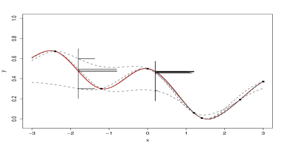
Figure 1: Illustration of the UP distribution. Dashed lines: CV sub-models predictions, solid red line: master model prediction, horizontal bars: local UP distribution at $x_{a}=-1.8$ and $x_{b}=0.2$, black squares: design points.

Notice that in the interval $[1,3]$ (where we have 4 design points) the discrepancy between the master model and the CV sub-models predictions is smaller than in the remaining space. Moreover, we displayed horizontally the UP distribution at $x_{a}=-1.8$ and $x_{b}=0.2$ to illustrate the weighting effect. One can notice that:

• At $x_{a}$ the least weighted predictions are $\hat{s}_{n,-1}(x_{a})$ and $\hat{s}_{n,-2}(x_{a})$. These predictions do not use the two closest design points to $x_{a}$ : ($x_{1}$, respectively $x_{2}$).

• At $x_{b}$, $\hat{s}_{n,-3}(x_{b})$ is the least weighted prediction.

Furthermore, we display in Figure 2 the master model prediction and region delimited by $\hat{s}_{n}(\mathbf{x})+3\hat{\sigma}_{n}(\mathbf{x})$ and $\hat{s}_{n}(\mathbf{x})-3\hat{\sigma}_{n}(\mathbf{x})$.

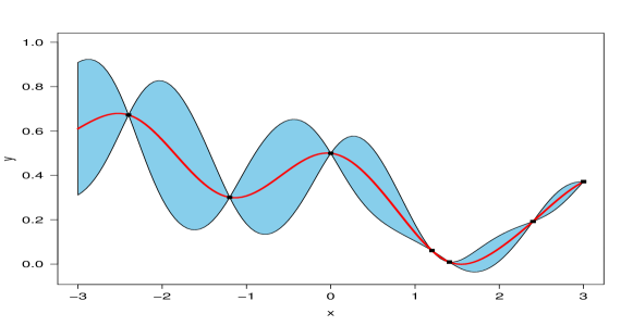
Figure 2: Uncertainty quantification based on the UP distribution. Red solid line: master model prediction $\hat{s}_{n}(\mathbf{x})$, blue area: region delimited by $\hat{s}_{n}(\mathbf{x})\pm 3\hat{\sigma}_{n}(\mathbf{x})$.

One can notice that the standard deviation is null at design points. In addition, its local maxima in the interval $[1,3]$ (where we have more design points density) are smaller than its maxima in the remaining space region.

4 Sequential Refinement

In this section, we use the UP distribution to define an adaptive refinement technique called the Universal Prediction-based Surrogate Modeling Adaptive Refinement Technique UP-SMART.

4.1 Introduction

The main goal of sequential design is to minimize the number of calls of a computationally expensive function. Gaussian surrogate models [18] are widely used in adaptive design strategies. Indeed, Gaussian modeling gives a Bayesian framework for sequential design. In some cases, other surrogate models might be more accurate although they do not provide a theoretical framework for uncertainty assessment. We propose here a new universal strategy for adaptive sequential design of experiments. The technique is based on the UP distribution. So, it can be applied to any type of surrogate model.

In the literature, many strategies have been proposed to design the experiments (for an overview, the interested reader is referred to [12, 40, 34]). Some strategies, such as Latin Hypercube Sampling (LHS) [28], maximum entropy design [35], and maximin distance designs [16] are called one-shot sampling methods. These methods depend neither on the output values nor on the surrogate model. However, one would naturally expect to design more points in the regions with high nonlinear behavior. This intuition leads to adaptive strategies. A DOE approach is said to be adaptive when information from the experiments (inputs and responses) as well as information from surrogate models are used to select the location of the next point.

By adopting this definition, adaptive DOE methods include for instance surrogate model-based optimization algorithms, probability of failure estimation techniques and sequential refinement techniques. Sequential refinement techniques aim at creating a more accurate surrogate model. For example, Lin et al. [25] use Multivariate Adaptive Regression Splines (MARS) and kriging models with Sequential Exploratory Experimental Design (SEED) method. It consists in building a surrogate model to predict errors based on the errors on a test set. Goel et al. [13] use an ensemble of surrogate models to identify regions of high uncertainty by computing the empirical standard deviation of the predictions of the ensemble members. Our method is based on the predictions of the CV sub-models. In the literature, several cross-validation-based techniques have been discussed. Li et al. [23] propose to add the design point that maximizes the Accumulative Error (AE). The AE on $\mathbf{x}\in\mathbb{X}$ is computed as the sum of the LOO-CV errors on the design points weighted by influence factors. This method could lead to clustered samples. To avoid this effect, the authors [24] propose to add a threshold constraint in the maximization problem. Busby et al. [6] propose a method based on a grid and CV. It affects the CV prediction errors at a design point to its containing cell in the grid. Then, an entropy approach is performed to add a new design point. More recently, Xu et al. [41] suggest the use of a method based on Voronoi cells and CV. Kleijnen et al.[19] propose a method based on the Jackknife’s pseudo values predictions variance. Jin et al. [15] present a strategy that maximizes the product between the deviation of CV sub-models predictions with respect to the master model prediction and the distance to the design points. Aute et al. [2] introduce the Space-Filling Cross-Validation Trade-off (SFCVT) approach. It consists in building a new surrogate model over LOO-CV errors and then add a point that maximizes the new surrogate model prediction under some space-filling constraints. In general cross-validation-based approaches tend to allocate points close to each other resulting in clustering [2]. This is not desirable for deterministic simulations.

4.2 UP-SMART

The idea behind UP-SMART is to sample points where the UP distribution variance (Equation (5)) is maximal. Most of the CV-based sampling criteria use CV errors. Here, we use the local predictions of the CV sub-models. Moreover, notice that the UP variance is null on design points for interpolating surrogate models. Hence, UP-SMART does not naturally promote clustering.

However, $\hat{\sigma}^{2}_{n}(\mathbf{x})$ can vanish even if $\mathbf{x}$ is not a design points. To overcome this drawback, we add a distance penalization. This leads to the UP-SMART sampling criterion $\gamma_{n}$ (Equation (7)).

$$\gamma_{n}(\mathbf{x})=\hat{\sigma}^{2}_{n}(\mathbf{x})+\delta\underline{d}_{\mathbf{X_{n}}}(\mathbf{x})$$ (7)

where $\delta>0$ is called exploration parameter. One can set $\delta$ as a small percentage of the global variation of the output. UP-SMART is the adaptive refinement algorithm consisting in adding at step $n$ a point $x_{n+1}\in\arg\max\limits_{\mathbf{x}\in\mathbb{X}}(\gamma_{n}(\mathbf{x}))$.

4.3 Performances on a set of test functions

In this subsection, we present the performance of the UP-SMART. We present first the used surrogate-models.

4.3.1 Used surrogate models

Kriging

Kriging  [27] or Gaussian process regression is an interpolation method.

Universal Kriging fits the data using a deterministic trend and governed by prior covariances. Let $k(\mathbf{x},\mathbf{x^{\prime}})$, be a covariance function on $\mathbb{X}\times\mathbb{X}$, and let $(h_{i})_{1\leq i\leq p}$ be the basis functions of the trend. Let us denote $\mathbf{h}(\mathbf{x})$ the vector $(h_{1}(\mathbf{x}),..,h_{p}(\mathbf{x}))^{\top}$ and let $H$ be the matrix with entries $h_{ij}=h_{j}(\mathbf{x_{i}}),1\leq i,j\leq n$. Furthermore, let $\mathbf{k_{n}}(\mathbf{x})$ be the vector $(k(\mathbf{x},\mathbf{x_{1}}),..,k(\mathbf{x},\mathbf{x_{n}}))^{\top}$ and $K_{n}$ the matrix with entries $k_{i,j}=k(\mathbf{x_{i}},\mathbf{x_{j}})$, for $1\leq i,j\leq n$.

Then, the conditional mean of the Gaussian process with covariance $k(\mathbf{x},\mathbf{x^{\prime}})$ and its variance are given in Equations ((8),(9))

$$m_{G_{n}}(\mathbf{x}) =\mathbf{h}(\mathbf{x})^{\top}\hat{\beta}+\mathbf{k_{n}}(\mathbf{x})^{\top}K_{n}^{-1}(Y-H^{\top}\hat{\beta})$$ (8)

$$\sigma^{2}_{GP_{n}}(\mathbf{x}) =k(\mathbf{x},\mathbf{x})-\mathbf{k_{n}}(\mathbf{x})^{\top}K_{n}^{-1}\mathbf{k_{n}}(\mathbf{x})^{\top}+\mathbf{V}(\mathbf{x})^{\top}(H^{\top}K_{n}^{-1}H)^{-1}\mathbf{V}(\mathbf{x})$$ (9)

$$\hat{\beta} =(H^{\top}K_{n}^{-1}H)^{-1}H^{\top}K_{n}^{-1}Y\text{ and }\mathbf{V}(\mathbf{x})=\mathbf{h}(\mathbf{x})^{\top}+\mathbf{k_{n}}(\mathbf{x})^{\top}K_{n}^{-1}H$$ (10)

Note that the conditional mean is the prediction of the Gaussian process regression. Further, we used two kriging instances with different sampling schemes in our test bench. Both use constant trend function and a Matérn 5/2 covariance function. The first design is obtained by maximizing the UP distribution variance (Equation (5)). And the second one is obtained by maximizing the kriging variance $\sigma^{2}_{GP_{n}}(\mathbf{x})$.

Genetic aggregation

The genetic aggregation response surface is a method that aims at selecting the best response surface for a given design of experiments. It solves several surrogate models, performs aggregation and selects the best response surface according to the cross-validation errors.

The use of such response surface, in this test bench, aims at checking the universality of the UP distribution: the fact that it can be applied for all types of surrogate models.

4.3.2 Test bench

In order to test the performances of the method we launched different refinement processes for the following set of test functions:

• Branin: $f_{b}(x_{1},x_{2})=(x_{2}-(\frac{5.1}{4\pi^{2}})x_{1}^{2}+(\frac{5}{\pi})x_{1}-6)^{2}+10(1-(\frac{1}{8\pi}))\cos(x_{1})+10$.

• Six-hump camel: $f_{c}(x_{1},x_{2})=\left(4-2.1x_{1}^{2}+\frac{x_{1}^{4}}{3}\right)x_{1}^{2}+x_{1}x_{2}+x_{2}^{2}(4x_{2}^{2}-4)$.

• Hartmann6: $f_{h}(\mathbf{X}=(x_{1},\dots,x_{6}))=-\sum\limits_{i=1}^{4}\alpha_{i}\exp\Big{(}-\sum\limits_{j=0}^{6}A_{ij}(x_{j}-P_{ij})^{2}\Big{)}$. $A$,$P$ and $\alpha$ can be found in [9].

• Viana: (Equation (6))

For each function we generated by optimal Latin hyper sampling design the number of initial design points $n_{0}$, the number of refinement points $N_{max}$. We also generated a set of $N_{t}$ test points and their response $Z^{(t)}=(X^{(t)},Y^{(t)})$. The used values are available in Table 1.

Table 1: Used test functions

Function	dimension $d$	$n_{0}$	$N_{max}$	$N_{t}$
Viana	1	5	7	500
Branin	2	10	10	1600
Camel	2	20	10	1600
Hartmann6	6	60	150	10000

We fixed $n_{0}$ in order to get non-accurate surrogate models at the first step. Usually, one follows the rule-of-thumb $n_{0}=10\times d$ proposed in [26]. However, for Branin and Viana functions, this rule leads to a very good initial fit. Therefore, we choose lower values.

• Kriging variance-based refinement process (Equation (9)) as refinement criterion.

• Kriging using the UP-SMART: UP-variance as refinement criterion (Equation (7)).

• Genetic aggregation using the UP-SMART: UP-variance as refinement criterion (Equation (7)).

4.3.3 Results

For each function, we compute at each iteration the Q squared ($Q^{2}$) of the predictions of the test set $Z^{(t)}$ where $Q^{2}(\hat{s},Z^{(t)})=1-\frac{\sum\limits_{i=1}^{N_{t}}(y_{i}^{(t)}-\hat{s}(\mathbf{x_{i}}^{(t)}))^{2}}{\sum\limits_{i=1}^{N_{t}}(y_{i}^{(t)}-\bar{y})^{2}}$ and $\bar{y}=\frac{1}{N_{t}}\sum\limits_{i=1}^{N_{t}}y_{i}^{(t)}$. We display in Figure 3 the performances of the three different techniques described above for Viana (Figure 3a), Branin (Figure 3b) and Camel (Figure 3c) functions measured by $Q^{2}$ criterion.

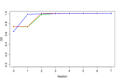
(a)

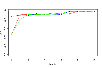
(b)

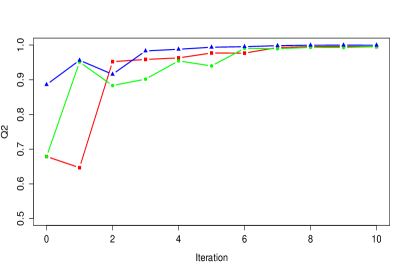
(c)

Figure 3: Performance of three refinement strategies on three test functions measured by the $Q^{2}$ criterion on a test set. x axis: number of added refinement points. y axis: $Q^{2}$. UP-SMART with kriging in green, UP-SMART with genetic aggregation in blue and kriging variance-based technique in red.

For these tests, the three techniques have comparable performances. The $Q^{2}$ converges for all of them. It appears that the UP variance criterion refinement process gives at least as good a result as the kriging variance criterion. This may be due to the high kriging uncertainty on the boundaries. In fact, minimizing kriging variance sampling algorithm generates, in general, more points on the boundaries for a high dimensional problem. For instance, let us focus on the Hartmann function (dimension 6). We present, in Figure 4, the results after 150 iterations of the algorithms. It is clear that the UP-SMART gives a better result for this function.

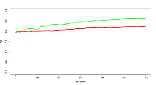
Figure 4: Performance of two refinement strategies on Hartmann function measured by the $Q^{2}$ criterion on a test set. x axis: number of added refinement points. y axis: $Q^{2}$. UP-SMART with kriging in green and kriging variance-based technique in red.

The results show that:

• UP-SMART gives a better global response surface accuracy than the maximization of the variance. This shows the usefulness of the method.

• UP-SMART is a universal method. Here, it has been applied with success to an aggregation of response surfaces. Such usage highlights the universality of the strategy.

5 Empirical Efficient Global optimization

In this section, we introduce UP distribution-based Efficient Global Optimization (UP-EGO) algorithm. This algorithm is an adaptation of the well known EGO algorithm.

5.1 Overview

Surrogate model-based optimization refers to the idea of speeding optimization processes using surrogate models. In this section, we present an adaptation of the well-known efficient global optimization (EGO) algorithm [17]. Our method is based on the weighted empirical distribution UP distribution. We show that asymptotically, the points generated by the algorithm are dense around the optimum. For the EGO al The proof has been done by Vazquez et al. [37] for the EGO algorithm.

The basic unconstrained surrogate model-based optimization scheme can be summarized as follows [30]

• Construct a surrogate model from a set of known data points.

• Define a sampling criterion that reflects a possible improvement.

• Optimize the criterion over the design space.

• Evaluate the true function at the criterion optimum/optima.

• Update the surrogate model using new data points.

• Iterate until convergence

Several sampling criteria have been proposed to perform optimization. The Expected Improvement (EI) is one of the most popular criteria for surrogate model-based optimization. Sasena et al. [33] discussed some sampling criteria such as the threshold-bounded extreme, the regional extreme, the generalized expected improvement and the minimum surprises criterion. Almost all of the criteria are computed in practice within the frame of Gaussian processes. Consequently, among all possible response surfaces, Gaussian surrogate models are widely used in surrogate model-based optimization. Recently, Viana et al. [39] performe multiple surrogate assisted optimization by importing Gaussian uncertainty estimate.

5.2 UP-EGO Algorithm

Here, we use the UP distribution to compute an empirical expected improvement. Then, we present an optimization algorithm similar to the original EGO algorithm that can be applied with any type of surrogate models. Without loss of generality, we consider the minimization problem:

$$\underset{\mathbf{x}\in\mathbb{X}}{\text{minimize}} s(\mathbf{x})$$

Let $(y(\mathbf{x}))_{\mathbf{x}\in\mathbb{X}}$ be a Gaussian process model. $m_{G_{n}}$ and $\sigma^{2}_{GP_{n}}$ denote respectively the mean and the variance of the conditional process $y(\mathbf{x})\mid\mathbf{Z_{n}}$. Further, let $y_{n}^{\star}$ be the minimum value at step $n$ when using observations $\mathbf{Z_{n}}=(z_{1},\dots,z_{n})$ where $z_{i}=(\mathbf{x_{i}},y_{i})$. ($y_{n}^{\star}=\min\limits_{i=1..n}{y_{i}}$). The EGO algorithm [17] uses the expected improvement $EI_{n}$ (Equation (11)) as sampling criterion:

$$EI_{n}(\mathbf{x})=\mathbb{E}[\max(y_{n}^{\star}-y(\mathbf{x}),0)\mid\mathbf{Z_{n}}]$$ (11)

The EGO algorithm adds the point that maximizes $EI_{n}$ . Using some Gaussian computations, Equation (11) is equivalent to Equation (12).

$$EI_{n}(\mathbf{x})=\left\{\begin{aligned} (y_{n}^{\star}-m_{G_{n}}(\mathbf{x}))\Phi\left(\frac{y_{n}^{\star}-m_{G_{n}}(\mathbf{x})}{\sigma_{GP_{n}}(\mathbf{x})}\right)+\sigma_{GP_{n}}(\mathbf{x})\phi\left(\frac{y_{n}^{\star}-m_{G_{n}}(\mathbf{x})}{\sigma_{GP_{n}}(\mathbf{x})}\right)&&\text{if }\sigma_{GP_{n}}(\mathbf{x})\neq 0\\ 0&&\text{otherwise}\\ \end{aligned}\right.$$ (12)

We introduce a similar criterion based on the UP distribution. With the notations of Sections 2 and 3, $EEI_{n}$ (Equation (13)) is called the empirical expected improvement.

$$EEI_{n}(\mathbf{x}) =\int\max(y_{n}^{\star}-y,0)\mu_{(n,\mathbf{x})}(dy)$$ (13)

$$=\sum\limits_{i=1}w_{i,n}(\mathbf{x})\max(y_{n}^{\star}-\hat{s}_{n,-i}(\mathbf{x}),0)$$

We can remark that $EEI_{n}(\mathbf{x})$ can vanish even if $\mathbf{x}$ is not a design point. This is one of the limitations of the empirical UP distribution. To overcome this drawback, we suggest the use of the Universal Prediction Expected Improvement (UP-EI) $\kappa_{n}$ (Equation (14) )

$$\kappa_{n}(\mathbf{x})=EEI_{n}(\mathbf{x})+\xi_{n}(\mathbf{x})$$ (14)

where $\xi_{n}(\mathbf{x})$ is a distance penalization. We use $\xi_{n}(\mathbf{x})=\delta\underline{d}_{\mathbf{X_{n}}}(\mathbf{x})$ where $\delta>0$ is called the exploration parameter. One can set $\delta$ as a small percentage of the global variation of the output for less exploration. Greater value of $\delta$ means more exploration. $\delta$ fixes the wished trade-off between exploration and local search.

Furthermore, notice that $\kappa_{n}$ has the desirable property also verified by the usual EI:

Proposition 5.1.

$\forall n>1,\forall\mathbf{Z_{n}}=(\mathbf{X_{n}}=(\mathbf{x_{1}},\dots,\mathbf{x_{n}})^{\top},\mathbf{Y_{n}}=s(\mathbf{X_{n}})),$ if the used model interpolates the data then $\kappa_{n}(\mathbf{x_{i}})=0$, for $i=1,\dots,n$

The UP distribution-based Efficient Global Optimization (UP-EGO) (Algorithm 1 ) consists in sampling at each iteration the point that maximize $\kappa_{n}$. The point is then added to the set of observations and the surrogate model is updated.

Algorithm 1.

UP-EGO(${\hat{s}}$)
     Inputs: $\mathbf{Z}_{n_{0}}=(X_{n_{0}},Y_{n_{0}})$, $n_{0}\in\mathbb{N}\setminus\{0,1\}$ and a deterministic function $s$
$\text{ }\hskip 15.0pt(1)$ $m:=n_{0}$, $\mathbf{S}_{m}:=X_{n_{0}}$, $Y_{m}:=Y_{n_{0}}$
$\text{ }\hskip 15.0pt(2)$ Compute the surrogate model $\hat{s}_{\mathbf{Z}_{m}}$
$\text{ }\hskip 15.0pt(3)$ Stop_conditions $:=$ False
$\text{ }\hskip 15.0pt(4)$While Stop_conditions are not satisfied

$\text{ }\hskip 40.0pt(4.1)$ Select $\mathbf{x_{m+1}}\in arg\max\limits_{\mathbb{X}}(\kappa_{m}(\mathbf{x}))$

$\text{ }\hskip 40.0pt(4.2)$ Evaluate $y_{m+1}:=s(\mathbf{x_{m+1}})$

$\text{ }\hskip 40.0pt(4.3)$ $\mathbf{S}_{m+1}:=\mathbf{S}_{m}\cup\{\mathbf{x_{m+1}}\}$, $Y_{m+1}:=Y_{m}\cup\{y_{m+1}\}$

$\text{ }\hskip 40.0pt(4.4)$ $\mathbf{Z}_{m+1}:=(\mathbf{S}_{m+1},Y_{m+1})$,$m:=m+1$

$\text{ }\hskip 40.0pt(4.5)$ Update the surrogate model

$\text{ }\hskip 40.0pt(4.6)$ Check Stop_conditions
        end loop
    Outputs: $\mathbf{Z}_{m}:=(\mathbf{S}_{m},Y_{m})$, surrogate model $\hat{s}_{\mathbf{Z}_{m}}$

5.3 UP-EGO convergence

We first recall the context. $\mathbb{X}$ is a nonempty compact subset of the Euclidean space $\mathbb{R}^{p}$ where $p\in\mathbb{N}^{\star}$. $s$ is an expensive-to-evaluate function. The weights of the UP distribution are computed as in Equation (2) with $\rho>0$ a fixed real parameter. Moreover, we consider the asymptotic behaviour of the algorithm so that, here, the number of iterations goes to infinity.

Let $\mathbf{x^{\star}}\in\operatorname*{arg\,min}\{s(\mathbf{x}),\mathbf{x}\in\mathbb{X}\}$ and $\hat{s}$ be a continuous interpolating surrogate model bounded on $\mathbb{X}$. Let $\mathbf{Z}_{n_{0}}=(X_{n_{0}}=(\mathbf{x_{1}},\dots,\mathbf{x_{n_{0}}})^{\top},Y_{n_{0}})$ be the initial data. For all $k>n_{0}$, $\mathbf{x_{k}}$ denotes the point generated by the UP-EGO algorithm at step $k-n_{0}$. Let $\mathbf{S}_{m}$ denote the set $\{\mathbf{x_{i}},i\leq m\}$ and $S=\{\mathbf{x_{i}},i>0\}$. Finally, $\forall m>n_{0}$ we note $\kappa_{m}$ the UP-EI of $\hat{s}_{\mathbf{Z}_{m}}$. We are going to prove that $\mathbf{x^{\star}}$ is adherent to the sequence $S$ generated by the UP-EGO($\hat{s}$) algorithm.

Lemma 5.2.

$\exists\theta>0$, $\forall m\geq n_{0}$, $\forall\mathbf{x}\in\mathbb{X}$, $\forall i\in 1,\dots,m$, $\forall n>m$, $w_{i,n}(\mathbf{x})\leq\theta d(\mathbf{x},\mathbf{x_{i}})^{2}$.

Definition 5.3.

A surrogate model $\hat{s}$ is called an interpolating surrogate model if for all $n\in\mathbb{N}^{\star}$ and for all $\mathbf{Z_{n}}=(\mathbf{X_{n}},\mathbf{Y_{n}})\in\mathbb{X}^{n}\times\mathbb{R}^{n}$, $\hat{s}_{\mathbf{Z_{n}}}(\mathbf{x})=s(\mathbf{x})$ if $\mathbf{x}\in\mathbf{X_{n}}$.

Definition 5.4.

A surrogate model $\hat{s}$ is called bounded on $\mathbb{X}$ if for all $s$ a continuous function on $\mathbb{X}$, $\exists L,U$, such that for all $n>1$ and for all $\mathbf{Z_{n}}=(\mathbf{X_{n}},\mathbf{Y_{n}}=s(\mathbf{X_{n}}))\in\mathbb{X}^{n}\times\mathbb{R}^{n}$, $\forall\mathbf{x}\in\mathbb{X}$, $L\leq\hat{s}_{\mathbf{Z_{n}}}(\mathbf{x})\leq U$

Definition 5.5.

A surrogate model $\hat{s}$ is called continuous if $\forall n_{0}>1$ $\forall\mathbf{x}\in\mathbb{X}$ $\forall\varepsilon>0$, $\exists\delta>0$, $\forall n\geq n_{0}$, $\forall\mathbf{Z_{n}}=(\mathbf{X_{n}},\mathbf{Y_{n}})\in\mathbb{X}^{n}\times\mathbb{R}^{n}$, $\forall\mathbf{x^{\prime}}\in\mathbb{X}$, $d(\mathbf{x},\mathbf{x^{\prime}})<\delta\implies\left|\hat{s}_{\mathbf{Z_{n}}}(\mathbf{x})-\hat{s}_{\mathbf{Z_{n}}}(\mathbf{x^{\prime}})\right|<\varepsilon$

Theorem 5.6.

Let $s$ be a real function defined on $\mathbb{X}$ and let $\mathbf{x^{\star}}\in\arg\min\{s(\mathbf{x}),\mathbf{x}\in\mathbb{X}\}$. If $\hat{s}$ is an interpolating continuous surrogate model bounded on $\mathbb{X}$, then $\mathbf{x^{\star}}$ is adherent to the sequence of points $S$ generated by UP-EGO(${\hat{s}}$).

The proofs (Section 9) show that the exploration parameter is important for this theoretical result. In our implementation, we scale the input spaces to be the hypercube $\big{[}-1,1]$ and we set $\delta$ to $0.005\%$ of the output variation. Hence, the exploratory effect only slightly impacts the UP-EI criterion in practical cases.

5.4 Numerical examples

Let us consider the set of test functions (Table 2).

Table 2: Optimization test functions

function $f^{(i)}$	Dimension $d^{(i)}$	Number of initial points $n_{0}^{(i)}$	Number of iterations $N_{max}^{(i)}$
Branin	2	5	40
Ackley	2	10	30
Six-hump Camel	2	10	30
Hartmann6	6	20	40

We launched the optimization process for these functions with three different optimization algorithms:

• EGO [17]: Implementation of the R package DiceOptim [32] using the default parameters.

• UP-EGO algorithm applied to a universal kriging surrogate model $\hat{s_{k}}$ that uses Matérn 5/2 covariance function and a constant trend function. We denote this algorithm UP-EGO($\hat{s_{k}}$)

• UP-EGO algorithm applied to the genetic aggregation $\hat{s_{a}}$. It is then denoted UP-EGO($\hat{s_{a}}$).

For each function $f^{(i)}$, we launched each optimization process for $N_{max}^{(i)}$ iterations starting with $N_{seed}=20$ different initial design of experiments of size $n_{0}^{(i)}$ generated by an optimal space-filling sampling. The results are given using boxplots in Appendix Appendix: Optimization test results. We also display the mean best value evolution in Figure 5.

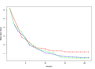
(a)

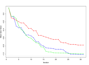
(b)

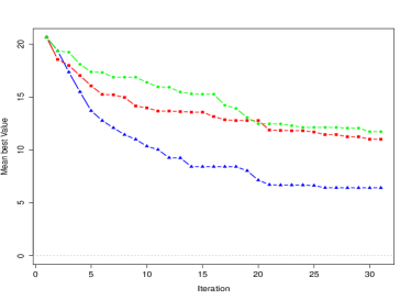
(c)

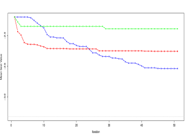
(d)

Figure 5: Comparison of three surrogate-based optimization strategies. Mean over $N_{seed}$ of the best value as a function of the number of iterations. UP-EGO with kriging in green, UP-EGO with genetic aggregation in blue, EGO in red and theoretical minimum in dashed gray.

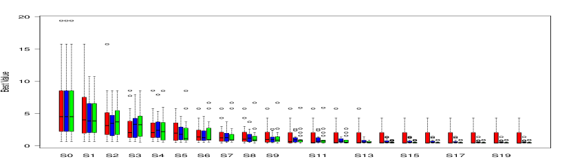
Figure 8: Branin: Box plots convergence

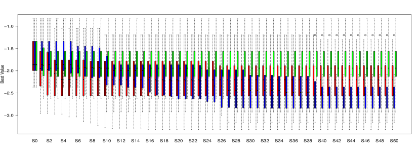
Figure 11: Hartmann6: Box plots convergence

The results shows that the UP-EGO algorithms give better results than the EGO algorithm for Branin and Camel functions. These cases illustrate the efficiency of the method. Moreover, for Ackley and Harmtann6 functions the best results are given by UP-EGO using the genetic aggregation. Even if this is related to the nature of the surrogate model, it underlines the efficient contribution of the universality of UP-EGO. Further, let us focus on the boxplots of the last iterations of Figures 8 and 11 (Appendix Appendix: Optimization test results). It is important to notice that UP-EGO results for Branin function depend slightly on the initial design points. On the other hand, let us focus on the Hartmann function case. The results of UP-EGO using the genetic aggregation depend on the initial design points. In fact, more optimization iterations are required for a full convergence. However, compared to the EGO algorithm, UP-EGO algorithm has good performances for both cases:

• Full convergence

• Limited-budget optimization.

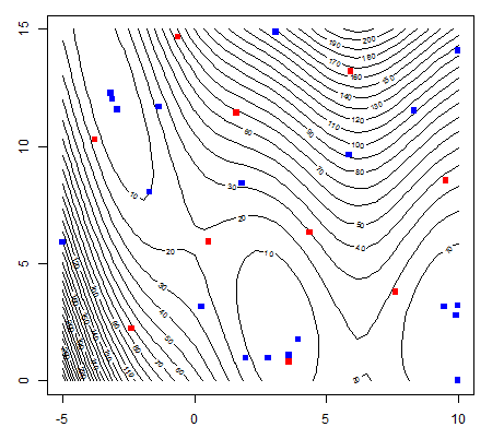
Figure 6: Example of sequence generated by by the UP-EGO(kriging) algorithm on Branin function. Initial design points are in red, added points are in blue.

Otherwise, the Branin function has multiple solutions. We are interested in checking whether the UP-EGO algorithm would focus on one local optimum or on the three possible regions. We present in Figure 6 the spatial distribution of the generated points by the UP-EGO(kriging) algorithm for the Branin function. We can notice that UP-EGO generated points around the three local minima.

6 Fluid Simulation Application: Mixing Tank

The problem addressed here concerns a static mixer where hot and cold fluid enter at variable velocities. The objective of this analysis is generally to find inlet velocities that minimize pressure loss from the cold inlet to the outlet and minimize the temperature spread at the outlet. In our study, we are interested in a better exploration of the design using an accurate cheap-to-evaluate surrogate model.

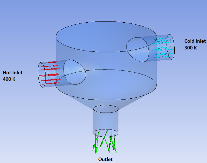
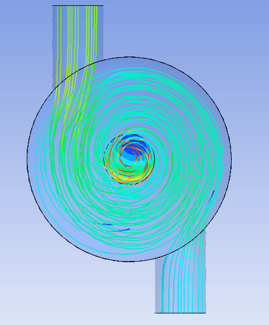
Figure 7: Mixing tank

The simulations are computed within ANSYS Workbench environment and we used DesignXplorer to perform surrogate-modeling. We started the study using 9 design points generated by a central composite design. We produced also a set of $N_{t}=80$ test points $Z_{t}=(X_{t}=(x_{1}^{(t)}),\dots,\mathbf{x}_{N_{t}}^{(t)}),Y_{t}=(y_{1}^{(t)}),\dots,y_{N_{t}}^{(t)}))$. We launched UP-SMART applied to the genetic aggregation response surface (GARS) in order to generate 10 suitable design points and a kriging-based refinement strategy. The genetic aggregation response surface (GARS) developed by DesignXplorer creates a mixture of surrogate models including support vector machine regression, Gaussian process regression, moving Least Squares and polynomial regression. We computed the root mean square error (Equation (15)), the relative root mean square error (Equation (16)) and the relative average absolute error (Equation (17)) before and after launching the refinement processes.

$$RMSE_{Z^{(t)}}(\hat{s}) =\frac{1}{N^{t}}\sum\limits_{i=1}^{N_{t}}(y_{i}^{(t)}-\hat{s}(\mathbf{x_{i}}^{(t)}))^{2}$$ (15)

$$RRMSE_{Z^{(t)}}(\hat{s}) =\frac{1}{N^{t}}\sum\limits_{i=1}^{N_{t}}\left(\frac{y_{i}^{(t)}-\hat{s}(\mathbf{x_{i}}^{(t)})}{y_{i}^{(t)}}\right)^{2}$$ (16)

$$RAAE_{Z^{(t)}}(\hat{s}) =\frac{1}{N^{t}}\sum\limits_{i=1}^{N_{t}}\frac{\mid y_{i}^{(t)}-\hat{s}(\mathbf{x_{i}}^{(t)})\mid}{\sigma_{Y}}$$ (17)

We give in Table 3 the obtained quality measures for the temperature spread output. In fact, the pressure loss is nearly linear and every method gives a good approximation.

Table 3: Quality measures of different response surfaces of static mixer simulations

Surrogate model	RRMSE	RMSE	RAAE
GARS Initial	0.16	0.10	0.50
GARS Final	0.10	0.07	0.31
Kriging Initial	0.16	0.11	0.48
Kriging Final	0.16	0.11	0.50

The results show that UP-SMART gives a better approximation. Here, it is used with a genetic aggregation of several response surface. Even if the good quality may be due to the response surface itself, it highlights the fact that UP-SMART made the use of such surrogate model-based refinement strategy possible.

7 Empirical Inversion

7.1 Empirical inversion criteria adaptation

Inversion approaches consist in the estimation of contour lines, excursion sets or probability of failure. These techniques are specially used in constrained optimization and reliability analysis.

Several iterative sampling strategies have been proposed to handle these problems. The empirical distribution $\mu_{n,\mathbf{x}}$ can be used for inversion problems. In fact, we can compute most of the well-known criteria such as the Bichon’s criterion [4] or the Ranjan’s criterion [31] using the UP distribution. In this section, we discuss some of these criteria: the targeted mean square error $TMSE$ [29], Bichon [4] and the Ranjan criteria [31]. The reader can refer to Chevalier et al. [7] for an overview.

Let us consider the contour line estimation problem : let $T$ be a fixed threshold. We are interested in enhancing the surrogate model accuracy in $\{\mathbf{x}\in\mathbb{X},s(\mathbf{x})=T\}$ and in its neighborhood.

Targeted MSE (TMSE)

The targeted Mean Square Error (TMSE) [29] aims at decreasing the mean square error where the kriging prediction is close to T.

It is the probability that the response lies inside the interval $\big{[}T-\varepsilon,T+\varepsilon\big{]}$ where the parameter $\varepsilon>0$ tunes the size of the window around the threshold $T$. High values make the criterion more exploratory while low values concentrate the evaluation around the contour line.

We can compute an estimation of the value of this criterion using the UP distribution (Equation (18)).

$$TMSE_{T,n}(\mathbf{x}) =\sum\limits_{i=1}^{n}w_{i,n}(\mathbf{x})1_{\big{[}T-\varepsilon,T+\varepsilon\big{]}}\big{(}\hat{s}_{n,-i}(\mathbf{x})\big{)}$$ (18)

$$=\sum\limits_{i=1}^{n}w_{i,n}(\mathbf{x})1_{\big{[}-\varepsilon,\varepsilon\big{]}}\big{(}\hat{s}_{n,-i}(\mathbf{x})-T\big{)}$$

Notice that the last criterion takes into account neither the variability of the predictions at $\mathbf{x}$ nor the magnitude of the distance between the predictions and $T$.

Bichon criterion

The expected feasibility defined in [4] aims at indicating how well the true value of the response is expected to be close to the threshold $T$.

The bounds are defined by $\varepsilon_{\mathbf{x}}$ which is proportional to the kriging standard deviation $\hat{\sigma}(\mathbf{x})$. Bichon proposes using $\varepsilon_{\mathbf{x}}=2\hat{\sigma}(\mathbf{x})$ [4].

This criterion can be extended to the case of the UP distribution. We define in Equation (19) $EF_{n}$ the empirical Bichon’s criterion where $\varepsilon_{\mathbf{x}}$ is proportional to the empirical standard deviation $\hat{\sigma}^{2}_{n}(\mathbf{x})$ (Equation (5)).

$$EF_{n}(\mathbf{x}) =\sum\limits_{i=1}^{n}w_{i,n}(\mathbf{x})(\varepsilon_{\mathbf{x}}-|T-\hat{s}_{n,-i}(\mathbf{x})|)1_{\big{[}-\varepsilon_{\mathbf{x}},\varepsilon_{\mathbf{x}}\big{]}}(\hat{s}_{n,-i}(\mathbf{x})-T)$$ (19)

Ranjan criterion

Ranjan et al. [31] proposed a criterion that quantifies the improvement $I_{Ranjan}(\mathbf{x})$ defined in Equation (20)

$$I_{Ranjan}(\mathbf{x})=\left(\varepsilon^{2}_{\mathbf{x}}-(y(\mathbf{x})-T)^{2}\right)1_{[-\varepsilon_{\mathbf{x}},\varepsilon_{\mathbf{x}}]}(y(\mathbf{x})-T)$$ (20)

where $\varepsilon_{\mathbf{x}}=\alpha\hat{\sigma}(\mathbf{x})$, and $\alpha>0$. $\varepsilon_{\mathbf{x}}$ defines the size of the neighborhood around the contour $T$.

It is possible to compute the UP distribution-based Ranjan’s criterion (Equation (21)). Note that we set $\varepsilon_{\mathbf{x}}=\alpha\hat{\sigma}^{2}_{n}(\mathbf{x})$.

$$\mathbb{E}\Big{[}I_{Ranjan}(\mathbf{x})\Big{]} =\sum\limits_{i=1}^{n}w_{i,n}(\mathbf{x})\Big{(}\varepsilon_{\mathbf{x}}^{2}-(\hat{s}_{n,-i}(\mathbf{x})-T)^{2}\Big{)}1_{[-\varepsilon_{\mathbf{x}},\varepsilon_{\mathbf{x}}]}(\hat{s}_{n,-i}(\mathbf{x})-T)$$ (21)

7.2 Discussion

The use of the pointwise criteria (Equations (18), (19), (21)) might face problems when the region of interest is relatively small to the prediction jumps. In fact, as the cumulative distribution function of the UP distribution is a step function, the probability of the prediction being inside an interval can vanish even if it is around the mean value. For instance $\mu_{n,\mathbf{x}}\big{(}y(\mathbf{x})\in[T-\varepsilon,T+\varepsilon]\big{)}$ can be zero. This is one of the drawbacks of the empirical distribution. Some regularization techniques are possible to overcome this problem. For instance, the technique that consists in defining the region of interest by a Gaussian density $\mathcal{N}(0,\sigma^{2}_{\varepsilon})$ [29]. Let $g_{\varepsilon}$ be this Gaussian probability distribution function.

The new $TMSE$ denoted $TMSE^{(2)}_{T,n}(\mathbf{x})$ criterion is then as in Equation (22).

$$TMSE^{(2)}_{T,n}(\mathbf{x})=\sum\limits_{i=1}^{n}w_{i,n}(\mathbf{x})g_{\varepsilon}\big{(}\hat{s}_{n,-i}(\mathbf{x})-T\big{)}$$ (22)

The use of the Gaussian density to define the targeted region seems more relevant when using the UP local varaince. Similarly, we can apply the same method to the Ranjan’s and Bichon’s criteria.

8 Conclusion

To perform surrogate model-based sequential sampling, several relevant techniques require to quantify the prediction uncertainty associated to the model. Gaussian process regression provides directly this uncertainty quantification. This is the reason why Gaussian modeling is quite popular in sequential sampling. In this work, we defined a universal approach for uncertainty quantification that could be applied for any surrogate model. It is based on a weighted empirical probability measure supported by cross-validation sub-models predictions.

Hence, one could use this distribution to compute most of the classical sequential sampling criteria. As examples, we discussed sampling strategies for refinement, optimization and inversion. Further, we showed that, under some assumptions, the optimum is adherent to the sequence of points generated by the optimization algorithm UP-EGO. Moreover, the optimization and the refinement algorithms were successfully implemented and tested both on single and multiple surrogate models. We also discussed the adaptation of some inversion criteria. The main drawback of UP distribution is that it is supported by a finite number of points. To avoid this, we propose to regularize this probability measure. In a future work, we will study and implement such regularization scheme and study the case of multi-objective constrained optimization.

9 Proofs

We present in this section the proofs of Proposition 5.1, Lemma 5.2 and Theorem 5.6. Here, we use the notations of Section 5.3.

Proposition 5.1.

Let $n>1$, $\mathbf{Z_{n}}=(\mathbf{X_{n}}=(\mathbf{x_{1}},\dots,\mathbf{x_{n}})^{\top},\mathbf{Y_{n}}=s(\mathbf{X_{n}})),$ and $\hat{s}$ a model that interpolates the data i.e $\forall i\in 1,\dots,n$, $\hat{s}_{\mathbf{Z_{n}}}(\mathbf{x_{i}})=s(\mathbf{x_{i}})=y_{i}$.

First, we have $\xi_{n}(\mathbf{x_{i}})=\delta\underline{d}_{\mathbf{X_{n}}}(\mathbf{x_{i}})$. Since $\mathbf{x_{i}}\in\mathbf{X_{n}}$ then $\xi_{n}(\mathbf{x_{i}})=0$ . Further, $EEI_{n}(\mathbf{x_{i}})=w_{i,n}(\mathbf{x_{i}})\max(y_{n}^{\star}-\hat{s}_{n,-i}(\mathbf{x_{i}}),0)+\sum\limits_{\begin{subarray}{c}j=1\\ j\neq i\end{subarray}}^{n}w_{j,n}(\mathbf{x_{i}})\max(y_{n}^{\star}-y_{i},0)$. Notice that $w_{i,n}(\mathbf{x_{i}})=0$ and $\max(y_{n}^{\star}-y_{i},0)=0$

Then $EEI_{n}(\mathbf{x_{i}})=0$. Finally, $\kappa_{n}(\mathbf{x_{i}})=EEI_{n}(\mathbf{x_{i}})+\xi_{n}(\mathbf{x_{i}})=0$. ∎

Lemma 5.2.

Let us note :

• $\phi_{\rho}(\mathbf{x},\mathbf{x^{\prime}})=1-e^{-\frac{d((\mathbf{x},\mathbf{x^{\prime}}))^{2}}{\rho^{2}}}$.

• $w_{i,n}(\mathbf{x})=\frac{\phi_{\rho}(\mathbf{x},\mathbf{x_{i}})}{\sum\limits_{k=1}^{n}\phi_{\rho}(\mathbf{x},\mathbf{x_{k}})}$.

Convex inequality gives $\forall a\in\mathbb{R}$, $1-e^{-a}<a$ then $\phi_{\rho}(\mathbf{x},\mathbf{x_{k}})\leq\frac{d((\mathbf{x},\mathbf{x_{k}}))^{2}}{\rho^{2}}$. Further, let $\mathbf{x_{k_{1}}},\mathbf{x_{k_{2}}}$ be two different design points of $X_{n_{0}}$, $\forall\mathbf{x}\in\mathbb{X}$, $\max\limits_{i\in\{1,2\}}\{d(\mathbf{x},\mathbf{x_{k_{i}}})\}\geq\frac{d(\mathbf{x_{k_{1}}},\mathbf{x_{k_{2}}})}{2}$ otherwise the triangular inequality would be violated. Consequently,

$\forall n>n_{0}$, $\sum\limits_{k=1}^{n}\phi_{\rho}(\mathbf{x},\mathbf{x_{k}})\geq\phi_{\rho}(\mathbf{x},\mathbf{x_{k_{1}}})+\phi_{\rho}(\mathbf{x},\mathbf{x_{k_{2}}})\geq\phi_{2\rho}(\mathbf{x_{k_{1}}},\mathbf{x_{k_{2}}})>0$

$\forall n>n_{0}$, $\forall\mathbf{x}\in\mathbb{X}$: $w_{i,n}(\mathbf{x})=\frac{\phi_{i,n}(\mathbf{x})}{\sum\limits_{k=1}^{n}\phi_{k,n}(\mathbf{x})}\leq\frac{\phi_{i,n}(\mathbf{x})}{\phi_{2\rho}(\mathbf{x_{k_{1}}},\mathbf{x_{k_{2}}})}\leq\frac{d((\mathbf{x},\mathbf{x_{i}}))^{2}}{\rho^{2}\phi_{2\rho}(\mathbf{x_{k_{1}}},\mathbf{x_{k_{2}}})}$

Considering $\theta=\frac{1}{\rho^{2}\phi_{2\rho}(\mathbf{x_{k_{1}}},\mathbf{x_{k_{2}}})}$ ends the proof. ∎

Theorem 5.6.

$\mathbb{X}$ is compact so $S$ has a convergent sub-sequence in $\mathbb{X}^{\mathbb{N}}$ (Bolzano-Weierstrass theorem ). Let $(x_{\psi(n)})$ denote that sub-sequence and $\mathbf{x_{\infty}}\in\mathbb{X}$ its limit. We can assume by considering a sub-sequence of $\psi$ and using the continuity of the surrogate model $\hat{s}$ that:

• $d(\mathbf{x_{\infty}},\mathbf{x}_{\psi(n)})\leq\frac{1}{n}$ for all $n>0$

• $\exists\nu_{n}\geq d(\mathbf{x_{\infty}},\mathbf{x}_{\psi(n)})$ such that $\forall\mathbf{x^{\prime}}\in\mathbb{X}$, $d(\mathbf{x^{\prime}},\mathbf{x_{\infty}})\leq\nu_{n}\implies\left|\hat{s}_{m,-i}(\mathbf{x_{\infty}})-\hat{s}_{m,-i}(\mathbf{x^{\prime}})\right|\leq\frac{1}{n},$ $\forall i\in 1,\dots,m$, where $m>n_{0}$.

For all $k>1$, we note $v_{k}=\psi(k+1)-1$, the step at which UP-EGO algorithm selects the point $\mathbf{x}_{\psi(k+1)}$. So, $\kappa_{v_{k}}(\mathbf{x}_{\psi(k+1)})=\max\limits_{\mathbf{x}\in\mathbb{X}}\{\kappa_{v_{k}}(\mathbf{x})\}$.

Notice first that for all $n>0$, $\mathbf{x}_{\psi(n)},\mathbf{x}_{\psi(n+1)}\in\mathcal{B}(\mathbf{x_{\infty}},\frac{1}{n})$ where $\mathcal{B}(\mathbf{x_{\infty}},\frac{1}{n})$ is the closed ball of center $\mathbf{x_{\infty}}$ and radius $\frac{1}{n}$. So:

$$\xi_{v_{n}}(\mathbf{x}_{\psi(n+1)})=\delta\underline{d}_{X_{v_{n}}}(\mathbf{x}_{\psi(n+1)})\leq\delta d(\mathbf{x_{\psi(n)}},\mathbf{x}_{\psi(n+1)})\leq\frac{2\delta}{n}$$ (i)

According to Lemma 5.2, $w_{\psi(n),v_{n}}\leq\theta\left(d(\mathbf{x}_{\psi(n+1)},\mathbf{x}_{\psi(n)})\right)^{2}$ so $w_{\psi(n),v_{n}}\leq\frac{4\theta}{n^{2}}$. Consequently:

$$w_{\psi(n),v_{n}}(\mathbf{x}_{\psi(n+1)})\max(y_{v_{n}}^{\star}-\hat{s}_{v_{n},-\psi(n)}(\mathbf{x}_{\psi(n+1)}),0)\leq\frac{4\theta(U-L)}{n^{2}}$$ (ii)

Further, $\forall i\in 1,\dots,v_{n}$, $i\neq\psi(n)$, $\hat{s}_{v_{n},-i}(\mathbf{x}_{\psi(n)})=y_{\psi(n)}$ since the surrogate model is an interpolating one. hence $\hat{s}_{v_{n},-i}(\mathbf{x}_{\psi(n)})\geq y_{v_{n}}^{\star}$ and so $\max(y_{v_{n}}^{\star}-\hat{s}_{v_{n},-i},0)\leq\max(\hat{s}_{v_{n},-i}(\mathbf{x}_{\psi(n)})-\hat{s}_{v_{n},-i}(\mathbf{x}_{\psi(n+1)}),0)\leq\left|\hat{s}_{v_{n},-i}(\mathbf{x}_{\psi(n)})-\hat{s}_{v_{n},-i}(\mathbf{x}_{\psi(n+1)})\right|$. Triangular inequality gives: $\max(y_{v_{n}}^{\star}-\hat{s}_{v_{n},-i},0)\leq\left|\hat{s}_{v_{n},-i}(\mathbf{x}_{\psi(n)})-\hat{s}_{v_{n},-i}(\mathbf{x}_{\infty})\right|+\left|\hat{s}_{v_{n},-i}(\mathbf{x}_{\infty})-\hat{s}_{v_{n},-i}(\mathbf{x}_{\psi(n+1)})\right|$ and finally:

$$\max(y_{v_{n}}^{\star}-\hat{s}_{v_{n},-i},0)\leq\frac{2}{n}$$ (iii)

We have:

$$\left|\kappa_{v_{n}}(\mathbf{x}_{\psi(n+1)})\right| =\xi_{v_{n}}(\mathbf{x}_{\psi(n+1)})+\sum\limits_{i=1}^{v_{n}}w_{i,v_{n}}(\mathbf{x}_{\psi(n+1)})\max(y_{v_{n}}^{\star}-\hat{s}_{v_{n},-i}(\mathbf{x}_{\psi(n+1)}),0)$$

$$=\xi_{v_{n}}(\mathbf{x}_{\psi(n+1)})+w_{\psi(n),v_{n}}(\mathbf{x}_{\psi(n+1)})\max(y_{v_{n}}^{\star}-\hat{s}_{v_{n},-\psi(n)}(\mathbf{x}_{\psi(n+1)}),0)$$

$$+\sum\limits_{\begin{subarray}{c}i=1\\ i\neq\psi(n)\end{subarray}}^{v_{n}}w_{i,v_{n}}(\mathbf{x}_{\psi(n+1)})\max(y_{v_{n}}^{\star}-\hat{s}_{v_{n},-i}(\mathbf{x}_{\psi(n+1)}),0)$$

$$\leq\frac{2\delta}{n}+\frac{4\theta(U-L)}{n^{2}}+\frac{2}{n}$$

Considering (i),(ii) and (iii) :

$$\left|\kappa_{v_{n}}(\mathbf{x}_{\psi(n+1)})\right|\leq\frac{2\delta}{n}+\frac{4\theta(U-L)}{n^{2}}+\frac{2}{n}\\$$

Notice that:
$\kappa_{v_{n}}(\mathbf{x}_{\psi(n+1)})=\max\limits_{\mathbf{x}\in\mathbb{X}}\{\kappa_{v_{n}}(\mathbf{x})\}$ and $\delta\underline{d}_{\mathbf{S}_{v_{n}}}(\mathbf{x^{\star}})=\xi_{v_{n}}(\mathbf{x^{\star}})$ $\leq\kappa_{v_{n}}(\mathbf{x^{\star}})\leq\kappa_{v_{n}}(\mathbf{x}_{\psi(n)})$. Since $\lim\limits_{n\to\infty}\left|\kappa_{v_{n}}(\mathbf{x}_{\psi(n+1)})\right|=0$ so $\lim\limits_{n\to\infty}\underline{d}_{\mathbf{S}_{v_{n}}}(\mathbf{x^{\star}})\to 0$. ∎

10 Acknowledgment

We gratefully acknowledge the French National Association for Research and Technology (ANRT, CIFRE grant number 2015/1349).

Appendix: Optimization test results

In this section, we use boxplots to display the evolution of the best value of the optimization test bench. For each iteration, we display: left: EGO in red., middle UP-EGO using genetic aggregation in blue, right: UP-EGO using kriging in green.

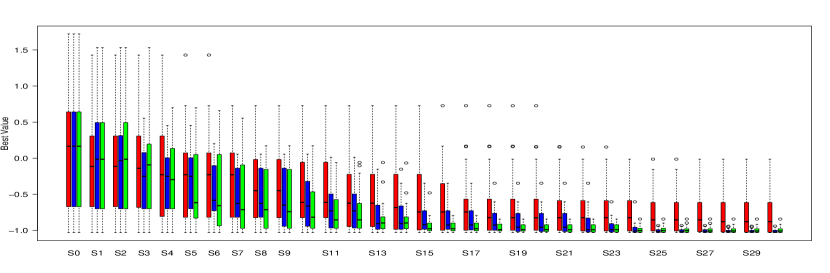
Figure 9: Six-hump camel: Box plots convergence

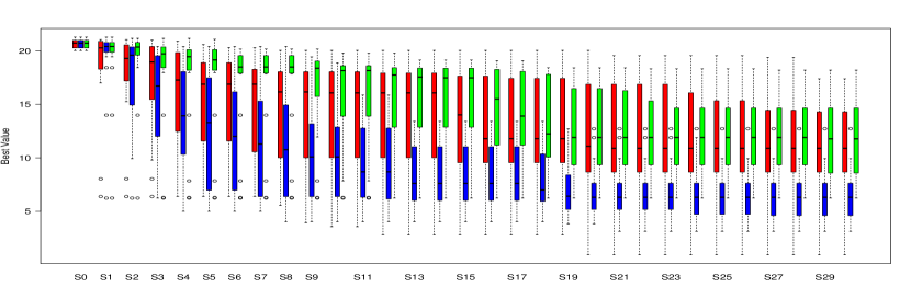
Figure 10: Ackley: Box plots convergence

References

- [1] S. Arlot and A. Celisse, A survey of cross-validation procedures for model selection, Statist. Surv., 4 (2010), pp. 40–79.
- [2] V. Aute, K. Saleh, O. Abdelaziz, S. Azarm, and R. Radermacher, Cross-validation based single response adaptive design of experiments for kriging metamodeling of deterministic computer simulations, Struct. Multidiscipl. Optim., 48 (2013), pp. 581–605.
- [3] J. Bect, D. Ginsbourger, L. Li, V. Picheny, and E. Vazquez, Sequential design of computer experiments for the estimation of a probability of failure, Stat. Comput., 22 (2012), pp. 773–793.
- [4] B. J. Bichon, M. S. Eldred, L.P. Swiler, S. Mahadevan, and J. M. McFarland, Efficient global reliability analysis for nonlinear implicit performance functions, AIAA journal, 46 (2008), pp. 2459–2468.
- [5] G.E.P. Box, W.G. Hunter, and J.S. Hunter, Statistics for experimenters: an introduction to design, data analysis, and model building, Wiley New York, 1978.
- [6] D. Busby, C.L. Farmer, and A. Iske, Hierarchical nonlinear approximation for experimental design and statistical data fitting, SIAM J. Sci. Comput., 29 (2007), pp. 49–69.
- [7] C. Chevalier, V. Picheny, and D. Ginsbourger, Kriginv: An efficient and user-friendly implementation of batch-sequential inversion strategies based on kriging, Comput. Statist. Data Anal., 71 (2014), pp. 1021 – 1034.
- [8] L.P. Devroye and T.J. Wagner, Distribution-free performance bounds for potential function rules, IEEE Trans. Inform. Theory, 25 (1979), pp. 601–604.
- [9] L.C.W. Dixon and G.P. Szegö, Towards global optimisation 2, North-Holland Amsterdam, 1978.
- [10] S. Gazut, J.-M. Martinez, G. Dreyfus, and Y. Oussar, Towards the optimal design of numerical experiments, IEEE Trans. Neural. Netw., 19 (2008), pp. 874–882.
- [11] S. Geisser, The predictive sample reuse method with applications, J. Amer. Statist. Assoc., 70 (1975), pp. 320–328.
- [12] A.A. Giunta, S.F. Wojtkiewicz, and M. S. Eldred, Overview of modern design of experiments methods for computational simulations, in Proceedings of the 41st AIAA aerospace sciences meeting and exhibit, AIAA-2003-0649, 2003.
- [13] T. Goel, R.T. Haftka, W. Shyy, and N.V. Queipo, Ensemble of surrogates, Struct. Multidiscip. Optim., 33 (2007), pp. 199–216.
- [14] D. Gorissen, T. Dhaene, and F. De Turck, Evolutionary model type selection for global surrogate modeling, J. Mach. Learn. Res., 10 (2009), pp. 2039–2078.
- [15] R. Jin, W. Chen, and A. Sudjianto, On sequential sampling for global metamodeling in engineering design, in Proc. ASME Des. Autom. Conf., American Society of Mechanical Engineers, 2002, pp. 539–548.
- [16] M.E. Johnson, L.M. Moore, and D. Ylvisaker, Minimax and maximin distance designs, J. Statist. Plann. Inference, 26 (1990), pp. 131–148.
- [17] D.R. Jones, M. Schonlau, and W.J. Welch, Efficient global optimization of expensive black-box functions, J. Global Optim., 13 (1998), pp. 455–492.
- [18] J.P.C. Kleijnen, Kriging metamodeling in simulation: A review, European J. Oper. Res., 192 (2009), pp. 707–716.
- [19] J.P.C Kleijnen and W.C.M. Van Beers, Application-driven sequential designs for simulation experiments: Kriging metamodeling, J. Oper. Res. Soc., 55 (2004), pp. 876–883.
- [20] J.P.C. Kleijnen, W. van Beers, and I. van Nieuwenhuyse, Expected improvement in efficient global optimization through bootstrapped kriging, J. Glob. Optim., 54 (2012), pp. 59–73.
- [21] D. G. Krige, A Statistical Approach to Some Basic Mine Valuation Problems on the Witwatersrand, J. South. Afr. Inst. Min. Metall., 52 (1951), pp. 119–139.
- [22] P Lancaster and K. Salkauskas, Surfaces generated by moving least squares methods, Math. Comp., 37 (1981), pp. 141–158.
- [23] G. Li and S. Azarm, Maximum accumulative error sampling strategy for approximation of deterministic engineering simulations, in Proc. AIAA-ISSMO Multidiscip. Anal. Optim. Conf., 2006.
- [24] G. Li, S. Azarm, A. Farhang-Mehr, and A.R. Diaz, Approximation of multiresponse deterministic engineering simulations: a dependent metamodeling approach, Struct. Multidiscipl. Optim., 31 (2006), pp. 260–269.
- [25] Y. Lin, F. Mistree, J.K. Allen, K.L Tsui, and V. Chen, Sequential metamodeling in engineering design, in Proc. AIAA-ISSMO Multidiscip. Anal. Optim. Conf., 2004.
- [26] Jason L Loeppky, Jerome Sacks, and William J Welch, Choosing the sample size of a computer experiment: A practical guide, Technometrics, 51 (2009).
- [27] G. Matheron, Principles of geostatistics, Econ. Geol., 58 (1963), pp. 1246–1266.
- [28] M.D. McKay, R.J. Beckman, and W.J. Conover, Comparison of three methods for selecting values of input variables in the analysis of output from a computer code, Technometrics, 21 (1979), pp. 239–245.
- [29] V. Picheny, D. Ginsbourger, O. Roustant, R.T. Haftka, and N.H. Kim, Adaptive designs of experiments for accurate approximation of a target region, AMSE. J. Mech. Des., 132 (2010), pp. 071008–071008–9.
- [30] N.V. Queipo, R.T. Haftka, W. Shyy, T. Goel, R. Vaidyanathan, and P.K. Tucker, Surrogate-based analysis and optimization, Prog. Aerosp. Sci., 41 (2005), pp. 1–28.
- [31] P. Ranjan, D. Bingham, and G. Michailidis, Sequential experiment design for contour estimation from complex computer codes, Technometrics, 50 (2008).
- [32] O. Roustant, D. Ginsbourger, and Y. Deville, Dicekriging, diceoptim: Two r packages for the analysis of computer experiments by kriging-based metamodeling and optimization, J. Stat. Softw., 51 (2012), pp. 1–55.
- [33] M. J. Sasena, P.Y. Papalambros, and P. Goovaerts, Metamodeling sampling criteria in a global optimization framework, in 8th Symp Multidiscip. Anal. Optim., American Institute of Aeronautics and Astronautics, 2000.
- [34] T. Shao and S. Krishnamurty, A clustering-based surrogate model updating approach to simulation-based engineering design, AMSE. J. Mech. Des., 130 (2008), pp. 041101–041101–13.
- [35] M.C. Shewry and H.P. Wynn, Maximum entropy sampling, J. Appl. Stat., 14 (1987), pp. 165–170.
- [36] A.J. Smola and B. Schölkopf, A tutorial on support vector regression, Stat. Comput., 14 (2004), pp. 199–222.
- [37] E Vazquez and J. Bect, Convergence properties of the expected improvement algorithm with fixed mean and covariance functions, J. Stat. Plan. Inference., 140 (2010), pp. 3088–3095.
- [38] F.A.C. Viana, R.T Haftka, and V. Steffen, Multiple surrogates: how cross-validation errors can help us to obtain the best predictor, Struct. Multidiscipl. Optim., 39 (2009), pp. 439–457.
- [39] F.A.C. Viana, R.T. Haftka, and L.T. Watson, Efficient global optimization algorithm assisted by multiple surrogate techniques, J. Glob. Optim., 56 (2013), pp. 669–689.
- [40] G.G. Wang and S. Shan, Review of metamodeling techniques in support of engineering design optimization, AMSE. J. Mech. Des., 129 (2007), pp. 370–380.
- [41] S. Xu, H. Liu, X. Wang, and X. Jiang, A robust error-pursuing sequential sampling approach for global metamodeling based on voronoi diagram and cross validation, AMSE. J. Mech. Des., 136 (2014), p. 071009.