Linear-Time Fitting of a $k$-Step Function

Abstract

Given a set of $n$ weighted points on the $x$-$y$ plane, we want to find a step function consisting of $k$ horizontal steps such that the maximum weighted vertical distance from any point to a step is minimized. Using the prune-and-search technique, we solve this problem in $O(n)$ time when $k$ is a constant. Our approach can be applied directly or with small modifications to solve other similar problems, such as the maximum error histogram problem and the line-constrained $k$-center problem, in $O(n)$ time when $k$ is a constant.

1 Introduction

Given an integer $k>0$ and a set $P$ of $n$ weighted points in the plane, our objective is to fit a $k$-step function to them so that the maximum weighted vertical distance of the points to the step function is minimized. We call this problem the $k$-step function problem. It has applications in areas such as geographic information systems, digital image analysis, data mining, facility locations, and data representation (histogram), etc.

In the unweighted case, if the points are presorted, Fournier and Vigneron [8] showed that the problem can be solved in linear time using the results of [10, 11, 12]. Later they showed that the weighted version of the problem can also be solved in $O(n\log n)$ time [9], using Megiddo’s parametric search technique [17]. Prior to these results, the problem had been discussed by several researchers [5, 7, 15, 16, 19].

Guha and Shim [13] considered this problem in the context of histogram construction. In database research, it is known as the maximum error histogram problem. In the weighted case, this problem is to partition the given points into $k$ buckets based on their $x$-coordinates, such that the maximum $y$-spread in each bucket is minimized. This problem is of interest to the data mining community as well (see [13] for references). Guha and Shim [13] computed the optimum histogram of size $k$, minimizing the maximum error. They present algorithms which run in linear time when the points are unweighted, and in $O(n\log n+k^{2}\log^{6}n)$ time and $O(n\log n)$ space when the points are weighted.

Our objective is to improve the above result to $O(n)$ time when $k$ is a constant. We show that we can optimally fit a $k$-step function to unsorted weighted points in linear time. We earlier suggested a possible approach to this problem at an OR workshop [3]. Here we flesh it out, presenting a complete and rigorous algorithm and proofs. Our algorithm exploits the well-known properties of prune-and-search along the lines in [2].

This paper is organized as follows. Section 2 introduces the notations used in the rest of this paper. It also briefly discusses how the prune-and-search technique can be used to optimally fit a $1$-step function (one horizontal line) to a given set of weighted points. We then consider in Section 3 a variant of the 2-step function problem, called the anchored 2-step function problem. We discuss a “big partition” in the context of the $k$-partition of a point set corresponding to a $k$-step function in Section 4. Section 5 presents our algorithm for the optimal $k$-step function problem. Section 6 concludes the paper, mentioning some applications of our results.

2 Preliminaries

2.1 Model

Let $P=\{p_{1},p_{2},\ldots,p_{n}\}$ be a set of $n$ weighted points in the plane. For $1\leq i\leq n$ let $p_{i}.x$ (resp. $p_{i}.y$) denote the $x$-coordinate (resp. $y$-coordinate) of point $p_{i}$, and let $w(p_{i})$ denote its weight. The points in $P$ are not sorted, except that $p_{1}.x\leq p_{i}.x\leq p_{n}.x$ holds for any $i=1,\ldots,n$. Let $F_{k}(x)$ denote a generic $k$-step function, whose $j^{th}$ segment (=step) is denoted by $s_{j}$. For $1\leq j\leq k-1$, segment $s_{j}$ represents a half-open horizontal interval $[s_{j}^{(l)},s_{j}^{(r)})$ between two points $s_{j}^{(l)}$ and $s_{j}^{(r)}$. The last segment $s_{k}$ represents a closed horizontal interval $[s_{k}^{(l)},s_{k}^{(r)}]$. Note that $s_{j}^{(l)}.y=s_{j}^{(r)}.y$, which we denote by $s_{j}.y$. We assume that for any $k$-step function $F_{k}(x)$, segments $s_{1}$ and $s_{k}$ satisfy $s_{1}^{(l)}.x=p_{1}.x$ and $s_{k}^{(r)}.x=p_{n}.x$, respectively. Segment $s_{j}$ is said to span a set of points $Q\subseteq P$, if $s_{j}^{(l)}.x\leq p.x<s_{j}^{(r)}.x$ holds for each $p\in Q$. A $k$-step function $F_{k}(x)$ gives rise to a $k$-partition of $P$, ${\cal P}=\{P_{j}\mid j=1,2,\ldots,k\}$, such that segment $s_{i}$ spans $P_{i}$. It satisfies the contiguity condition in the sense that for each partition $P_{j}$, if $a.x\leq b.x$ for $a,b\in P_{j}$, then every point $p$ with $a.x\leq p.x\leq b.x$ also belongs to $P_{j}$. In the rest of this paper, we consider only partitions that satisfy the contiguity condition. Fig. 1 shows an example of fitting a 4-step function $F_{4}(x)$.

Figure 1: Fitting a 4-step function.

Given a step function $F(x)$, defined over an $x$-range that contains $p.x$, let $d(p,F(x))$ denote the vertical distance of $p$ from $F(x)$. We define the cost of $p$ with respect to $F(x)$ by the weighted distance

$$D(p,F(x))\triangleq d(p,F(x))w(p).$$ (1)

We generalize the cost definition for a set $Q\subseteq P$ of points by

$$D(Q,F(x))\triangleq\max_{p\in Q}\{D(p,F(x))\}.$$ (2)

Point $p_{h}$ is said to be critical with respect to $F(x)$ if

$$D(p_{h},F(x))=D(P,F(x)).$$ (3)

Note that there can be more than one critical point with respect to a given step function. We similarly define a critical point with respect to a single segment of $F(x)$ as a point that has the maximum vertical weighted distance to it.

For a set of weighted points in the plane or on a line, the point that minimizes the maximum weighted distance to them is called the weighted 1-center [2]. Given a $k$-partition of $P$, ${\cal P}=\{P_{j}\mid j=1,2,\ldots,k\}$, it is clear that $\exists P_{i}\in{\cal P}$ such that $|P_{i}|\geq\lfloor n/k\rfloor$. We call any such partition a big partition. A big partition spanned by a segment in an optimal solution plays an important role. (See Procedure Big$({\cal P},k)$ in Sec. 4.3.)

2.2 Bisector

If we map each point $p_{i}\in P$ onto the $y$-axis, the cost of (or the weighted distance from) $p_{i}$ grows linearly from 0 at $p_{i}.y$ in each direction as a function of $y$. Consider arbitrary two points $p$ and $q$. Their costs intersect at either one or two points, one of which always lies between $p.y$ and $q.y$. If there are two intersections, the other intersection lies outside interval $[p.y,q.y]$ on the $y$-axis. If $p.y\not=q.y$ and $w(p)=w(q)$ hold then there is only one intersection. Let $a$ (resp. $b$) be the $y$-coordinate of the upper (resp. lower) intersection point, where $b\leq a$. We call the horizontal line $y=a$ (resp. $y=b$) the upper (resp. lower) bisector of $p$ and $q$. If there are only one intersection, we pretend that there were two at $b=a$, which lies between $p.y$ and $q.y$. (Note that the $y$-axis is shown horizontally in Figs. 2 and 3 below, where $y$ increases to the right.)

Let $\wp$ denote the $\lceil n/2\rceil$ pairs, formed by pairing up the points in $P$ arbitrarily. The cost lines of the points in each pair $(p,q)$ intersect as shown in Figs. 2.

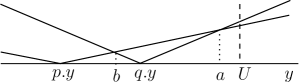
Figure 2: 1/3 of upper intersections are at $y<U$: (a) $p$ can be ignored at $y>U$; (b) $q$ can be ignored at $y>U$.

Let $y=U$ be the line at or above which at least 2/3 of the upper bisectors lie, and at or below which at least 1/3 of the upper bisectors lie. We use $\wp^{U}_{2/3}$ and $\wp^{U}_{1/3}$ to name the subsets of $\wp$ that have these two sets of bisectors, respectively. Note that $|\wp^{U}_{2/3}|\geq n/2\times 2/3=n/3$ and $|\wp^{U}_{1/3}|\geq n/2\times 1/3=n/6$. Similarly, let $y=L$ be the line at or below which at least 2/3 of the lower bisectors lie, and at or above which at least 1/3 of the bisectors lie. We use $\wp^{L}_{2/3}$ and $\wp^{L}_{1/3}$ to name the subsets of $\wp$ that have these two sets of bisectors, respectively. Note that $|\wp^{L}_{2/3}|\geq n/2\times 2/3=n/3$ and $|\wp^{L}_{1/3}|\geq n/2\times 1/3=n/6$.

Lemma 1.

We can identify $n/6$ points that can be removed without affecting the weighted 1-center for the values of their $y$-coordinates.

Proof.

Consider the following three possibilities.

1. The weighted 1-center lies above $U$.

2. The weighted 1-center lies below $L$.

3. The weighted 1-center lies between $U$ and $L$, including $U$ and $L$.

In case (i), there are two subcases, which are shown in Fig. 2(a) and (b), respectively. Since the center lies above $U$, we are interested in the upper envelope of the costs in the $y$-region given by $y>U$. In the case shown in Fig. 2(a), the costs of points $p$ and $q$ satisfy $d(y,p.y)w(p)<d(y,q.y)w(q)$ for $y>U$. Thus we can ignore $p$. In the case shown in Fig. 2(b), the costs of points $p$ and $q$ satisfy $d(y,p.y)w(p)>d(y,q.y)w(q)$ for $y>U$. Thus we can ignore $q$. Since $|\wp^{U}_{1/3}|\geq n/6$, in either case, one point from each such pair can be ignored, i.e., 1/6 of the points in $P$ can be eliminated, because it cannot affect the weighted 1-center. In case (ii) a symmetric argument proves that 1/6 of the points in $P$ can be discarded.

Figure 3: 2/3 of upper bisectors are at $y>U$.

In case (iii) see Fig. 3. The costs of each pair in $\wp^{U}_{2/3}$ (of the $2n/3$ pairs) as functions of $y$ intersect at most once at $y<U$. The cost functions of each pair in $\wp^{L}_{2/3}$ ($2n/3$ pairs) intersect at most once at $y>L$. Therefore, $\wp^{U}_{2/3}\cap\wp^{L}_{2/3}$ ($n/3$ pairs must be common to both,) i.e., both intersections of each such pair occur outside of the $y$-interval $[L,U]$. $|\wp^{U}_{2/3}\cap\wp^{L}_{2/3}|=n/2\times 1/3=n/6$. This implies that their cost functions do not intersect within in $[L,U]$, i.e., one of each pair lies above that of the other in $[L,U]$, and can be discarded. ∎

2.3 Optimal 1-step function

This problem is equivalent to finding the weighted center for $n$ points on a line. We pretend that all the points had the same $x$-coordinate. Then the problem becomes that of finding a weighted 1-center on a line, i.e., on the $y$-axis. This can be solved in linear time using Megiddo’s prune-and-search method [2, 4, 17]. In [18] Megiddo presents a linear time algorithm in the case where the points are unweighted. For the weighted case we now present a more technical algorithm that we can apply later to solve other related problems. The following algorithm uses a parameter $c$ which is a small integer constant.

Algorithm 1.

: 1-Step$(P)$

1. Pair up the points of $P$ arbitrarily.

2. For each such pair $(p,q)$ determine their horizontal bisector lines.

3. Determine a horizontal line, $y=U$ such that $|\wp^{U}_{2/3}|\geq n/3$ and $|\wp^{U}_{1/3}|\geq n/6$ hold.

4. Determine a horizontal line, $y=L$ such that $L$ $|\wp^{L}_{2/3}|\geq n/3$ and $|\wp^{L}_{1/3}|\geq n/6$ hold.

5. Determine the critical points for $U$ and $L$.

6. If there exist critical points for $U$ on both sides of (above and below) $U$, then $y=U$ defines an optimal 1-step function, $F^{*}_{1}(x)$; Stop. Otherwise, let $s_{U}$ (higher or lower than $U$) be the side of $U$ on which the critical point lies.

7. If there exist critical points for $L$ on both sides of $L$, $y=L$ defines $F^{*}_{1}(x)$; Stop. Otherwise, let $s_{L}$ (higher or lower than $L$) be the side of $L$ on which the critical point lies.

8. Based on $s_{U}$ and $s_{L}$, discard 1/6 of the points from $P$, based on Lemma 1.

9. If the size of the reduced set $P$ is greater than constant $c$, repeat this algorithm from the beginning with the reduced set $P$. Otherwise, determine $F^{*}_{1}(x)$ using any known method (which runs in constant time).

Lemma 2.

An optimal 1-step function $F^{*}_{1}(x)$ can be found in linear time.

Proof.

The recurrence relation for the running time $T(n)$ of 1-Step$(P)$ for general $n$ is $T(n)\leq T(n-n/6)+O(n)$, which yields $T(n)=O(n)$. ∎

3 Anchored $2$-step function problem

In general, we denote an optimal $k$-step function by $F^{*}_{k}(x)$ and its $i^{th}$ segment by $s^{*}_{i}$. Later, we need to constrain the first and/or the last step of a step function to be at a specified height. A $k$-step function is said to be left-anchored (resp. right-anchored), if $s_{1}.y$ (resp. $s_{k}.y$) is assigned a specified value, and is denoted by ${}^{\downarrow}\!F_{k}(x)$ (resp. $F_{k}^{\downarrow}(x)$). The anchored $k$-step function problem is defined as follows. Given a set $P$ of points and two $y$-values $a$ and $b$, determine the optimal $k$-step function ${}^{\downarrow}\!F^{*}_{k}(x)$ (resp. $F_{k}^{\downarrow*}(x)$) that is left-anchored (resp. right-anchored) at $a$ (resp. $b$) such that cost $D(P,^{\downarrow}\!\!F^{*}_{k}(x))$ (resp. $D(P,F_{k}^{\downarrow*}(x))$) is the smallest possible. If a $k$-step function is both left- and right-anchored, it is said to be doubly anchored and is denoted by ${}^{\downarrow}\!F_{k}^{\downarrow}(x)$.

3.1 Doubly anchored 2-step function

Suppose that segment $s_{1}$ (resp. $s_{2}$) is anchored at $a$ (resp. $b$). See Fig. 4(a).

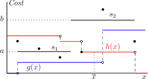
Figure 4: (a) $s_{1}.y=a$ and $s_{2}.y=b$; (b) Monotone functions $g(x)$ (in blue) and $h(x)$ (in red).

Let us define two functions $g(x)$ and $h(x)$ by

$$g(x) = \max_{p.x\leq x}\{w(p)\cdot|p.y-a|~{}\mid p\in P\},$$ (4)

$$h(x) = \max_{p.x>x}\{w(p)\cdot|p.y-b|~{}\mid p\in P\},$$ (5)

where $g(x)=0$ for $x<p_{1}.x$ and $h(x)=0$ for $x>p_{n}.x$. Intuitively, if we divide the points of $P$ at $x$ into two partitions $P_{1}$ and $P_{2}$, then $g(x)$ (resp. $h(x)$) gives the cost of partition $P_{1}$ (resp. $P_{2}$). See Fig. 4(b). Clearly the global cost for the entire $P$ is minimized for any $x$ at the lowest point in the upper envelope of $g(x)$ and $h(x)$, which is named $\overline{x}$. Since the points in $P$ are not sorted, $g(x)$ and $h(x)$ are not available explicitly, but we can compute $\overline{x}$ in linear time using the prune-and-search method, taking advantage of the fact that $\max\{g(x),h(x)\}$ is unimodal.

Algorithm 2.

: Doubly-Anch-2-Step$(P,a,b)$

1. Initialize $P^{\prime}=P$.

2. Find the point in $P^{\prime}$ that has the median $x$-coordinate, $x_{m}$.

3. Evaluate $g(x_{m})$ (resp. $h(x_{m})$) using (4) (resp. (5)).

4. If $g(x_{m})=h(x_{m})$ then $\overline{x}=x_{m}$. Stop.

5. If $g(x_{m})<h(x_{m})$ (resp. $g(x_{m})>h(x_{m})$), i.e., $\overline{x}<x_{m}$ (resp. $\overline{x}<x_{m}$), prune all the points $p$ with $p.x<x_{m}$ (resp. $p.x>x_{m}$), from $P^{\prime}$, remembering just the maximum cost.

6. Stop when $|P^{\prime}|=2$, and find the lowest point $\overline{x}$. Otherwise, go to Step 2.

We have the following lemma.

Lemma 3.

An optimal doubly anchored 2-step function can be found in linear time.

Proof.

Steps 2 and 3 of Algorithm Doubly-Anch-2-Step$(P,a,b)$ can be carried out in linear time. Since Step 4 cuts the size of $P^{\prime}$ in half every time, Step 2 is entered $O(\log n)$ times. Therefore the total time is $O(n)$. ∎

3.2 Left- or right-anchored 2-step function

Without loss of generality, we discuss only a left-anchored 2-step function. Given an anchor value $a$, we want to determine the optimal 2-step function with the constraint that $s^{*}_{1}.y=a$, denoted by ${}^{\downarrow}\!F^{*}_{2}(x)$. See Fig. 4(a). In this case, $b$ in (5) is not given; we need to find the optimal value for it. But assume for now that $b$ is also given, and execute Doubly-Anch-2-Step$(P,a,b)$. From the solution that it yields, can we find the direction in which to move $b$ to find the optimal left-anchored 2-step function?

Lemma 4.

Let $P_{1}$ (resp. $P_{2}$) be the left (resp right) partition of $P$ generated by Doubly-Anch-2-Step$(P,a,b)$ such that $s_{1}.y=a$ (resp. $s_{2}.y=b$), where $a<b$ without loss of generality. Assume that $P_{1}$ is maximal in the sense that the boundary between $P_{1}$ and $P_{2}$ cannot be moved to the right without increasing the cost of the solution.

1. If $D(P_{1},s_{1})\geq D(P_{2},s_{2})$ then the optimal right-anchor cannot lie above $y=b$.

2. If $D(P_{1},s_{1})<D(P_{2},s_{2})$ and there is a critical point in $P_{2}$ for $s_{2}.y=b$ above $y=b$, then the optimal right-anchor cannot lie below $y=b$.

3. If $D(P_{1},s_{1})<D(P_{2},s_{2})$ and there is a critical point in $P_{2}$ for $s_{2}.y=b$ below $y=b$, then the optimal right-anchor cannot lie above $y=b$.

Proof.

(a) Assume first that the critical point $p_{1}$ for $s_{1}$ lies below $s_{1}$ ($y=a$). Then we cannot reduce the cost by changing the value of $b$. Therefore, assume that $p_{1}$ lies above $s_{1}$. By the definition of $\{P_{1},P_{2}\}$, the leftmost point in $P_{2}$ lies above $y=b$, and moving the boundary between $P_{1}$ and $P_{2}$ to the right increases the cost, which is due to the weighted distance between $s_{1}$ and the new point in $P_{1}$, and this increase is independent of the value of $b$. Moving this boundary to the left cannot decrease the cost, until $p_{1}$ becomes a part of $P_{2}$, and even then a decrease is not possible unless $b$ is made smaller. Otherwise, $\{P_{1},P_{2}\}$ wouldn’t be optimal with the current $b$.

(b) We know that moving the boundary between $P_{1}$ and $P_{2}$ to the right increases the cost if $b$ is kept at the same value. The cost increases if $b$ is made smaller.

(c) Symmetric to Case (b). ∎

Figure 5: An example for $l$-Anch-2-Step$(P,a)$.

Example 1.

In Fig. 5, assume that $d_{2}$ is slightly larger than $d_{1}$. We have a doubly anchored solution with the minimum cost (weighted distance) equal to $d_{2}$. When the boundary between $P_{1}$ and $P_{2}$ is at $A$, we can reduce the cost of the optimal solution by moving $b$ up. We cannot do so if the boundary is at $B$, because $D(p_{3},s_{2})$ would increase. This is why we maximize $P_{1}$ in Step 5(b) of Algorithm 3 presented below. ∎

To make use of the prune-and-search method, we want to find the big partition (defined in Sec. 2.1), $P_{1}$ or $P_{2}$, that is spanned by one segment of ${}^{\downarrow}\!F^{*}_{2}(x)$. If $P_{1}$ is the big partition, we can eliminate all the points belonging to it, without affecting ${}^{\downarrow}\!F^{*}_{2}(x)$ that we will find. See Step 4 of the Algorithm 3 given below. We then repeat the process with the reduced set $P$. If $P_{2}$ is the big partition, on the other hand, we need to do more work, similar to what we did to find an optimal 1-step function. Namely, we determine values $U$ and $L$ for $P_{2}$ by executing Algorithm 1-Step$(P_{2})$. We then find a doubly anchored 2-step solution for $P$ with left anchor $a$ and right anchor $U$.

Algorithm 3.

: $l$-Anch-2-Step$(P,a)$

1. Divide $P$ into left partition $P_{1}$ and right partition $P_{2}$, whose sizes differ by at most one.

2. Let $s_{1}$ be the segment with $s_{1}.y=a$ spanning $P_{1}$, and let $s_{2}$ be the 1-step (optimal) solution for $P_{2}$.

3. If $D(P_{1},s_{1})=D(P_{2},s_{2})$ then output $\{s_{1},s_{2}\}$, which defines ${}^{\downarrow}\!F^{*}_{2}(x)$. Stop.

4. If $D(P_{1},s_{1})<D(P_{2},s_{2})$, remove from $P$ the points of $P_{1}$, except the critical point for $s_{1}$. Go to Step 6.

5. If $D(P_{1},s_{1})>D(P_{2},s_{2})$ then carry out the following steps.

   1. Determine points $U$ and $L$ for $P_{2}$ as described in Algorithm 1-Step$(P)$.

   2. Execute Doubly-Anch-2-Step$(P,a,U)$, and find the solution whose left partition is maximal. Repeat it with right anchor $L$.

   3. Eliminate 1/6 of the points of $P_{2}$ from $P$, based on the two solutions (as in Steps 6–8 of Algorithm 1-Step$(P)$.)

6. If $|P|>c$ (a small constant), repeat Steps 1 to 4. Otherwise, optimally solve the problem in constant time, using a known method.

In the example in Fig. 5, assume that $b$ is not given, and $s_{2}$ is determined by Step 2. Then we have $D(P_{1},s_{1})>D(P_{2},s_{2})$, and Step 5 applies. According to Step 5(a), we determine $U$. We then find the doubly anchored solution with the right anchor set to $b=U$.

Lemma 5.

Algorithm $l$-Anch-2-Step$(P,a)$ computes ${}^{\downarrow}\!F^{*}_{2}(x)$ correctly, and runs in linear time.

Proof.

Step 3 is obviously correct. If $D(P_{1},s_{1})<D(P_{2},s_{2})$ holds in Step 4, then the first partition of ${}^{\downarrow}\!F^{*}_{2}(x)$ contains $P_{1}$. We need to keep the critical point for $a$, but all other points of $P_{1}$ can be ignored from now on because $P_{1}$ will expand. If $D(P_{1},s_{1})>D(P_{2},s_{2})$ holds in Step 5, then the first partition of ${}^{\downarrow}\!F^{*}_{2}(x)$ is contained in $P_{1}$.

Each iteration of Steps 3 and 4 will eliminate at least $1/2\times 1/6=1/12$ of the points of $P$. Such an iteration takes linear time in the input size. The total time needed for all the iterations is therefore linear. ∎

4 $k$-step function

4.1 Approach

To design a recursive algorithm, assume that for any set of points $Q\subset P$, we can find the optimal $(j-1)$-step function and the optimal left- and right-anchored $j$-step function for any $2\leq j<k$ in $O(|Q|)$ time, where $k$ is a constant . We have shown that this is true for $k=2$ in the previous two sections. So the basis of induction holds.

Given an optimal $k$-step function $F^{*}_{k}(x)$, for each $i~{}(1\leq i\leq k)$, let $P^{*}_{i}$ be the set of points vertically closest to segment $s^{*}_{i}$. By definition, the partition $\{P^{*}_{i}\mid i=1,2,\ldots,k\}$ satisfies the contiguity condition. It is easy to see that for each segment $s^{*}_{i}$, there are (local) critical points with respect to $s^{*}_{i}$, lying on the opposite sides of $s^{*}_{i}$.

In finding an optimal $k$-step function, we first identify a big partition that will be spanned by a segment in an optimal solution. By Lemma 7, such a big partition always exists. Our objective is to eliminate a constant fraction of the points in a big partition. This will guarantee that a constant fraction of the input set is eliminated when $k$ is a fixed constant. The points in the big partition other than two critical points are “useless” and can be eliminated from further considerations. This elimination process is repeated until the problem size gets small enough to be solved by an exhaustive method in constant time.

4.2 Feasibility test

Given a weighted distance (=cost) $D$, a point set $P$ is said to be $D$-feasible if there exists a $k$-step function $F_{k}(x)$ such that $D(P,F_{k}(x))\leq D$. To test $D$-feasibility we first try to identify the first segment $s_{1}$ of a possible $k$-step function $F_{k}(x)$. To this end we compute the median $m$ of $\{p_{i}.x\mid i=1,2,\ldots,n\}$ in $O(n)$ time, and divide $P$ into two parts $P_{1}=\{p_{i}\mid p_{i}.x\leq m\}$ and $P_{2}=\{p_{i}\mid p_{i}.x>m\}$, which also takes $O(n)$ time. Note that $|P_{1}|\leq\lceil|P|/2\rceil$ and $|P_{2}|\leq\lceil|P|/2\rceil$ hold. We then find the intersection $I$ of the $y$-intervals in $\{|p_{i}.y-y|\leq D\mid p_{i}\in P_{1}\}$. Assuming that $P$ is $D$-feasible, then we have two cases.

Case (a): [$|I|=\emptyset$] $s_{1}$ ends at some point $p_{j}\in P_{1}$. Throw away all the points in $P_{2}$ and look for the longest $s_{1}$ limited by cost $D$, considering only the points in $P_{1}$ from the left.

Case (b): [$|I|\not=\emptyset$] $s_{1}$ may end at some point $p_{j}\in P_{2}$. Throw away all the points in $P_{1}$ and look for the longest $s_{1}$, using $I$ and the points in $P_{2}$ from the left.

Clearly, we can find the longest $s_{1}$ in $O(n)$ time. Remove the points spanned by $s_{1}$ from $P$, and find $s_{2}$ in $O(n)$ time, and so on. Since we are done after finding $k$ steps $\{s_{1},\ldots,s_{k}\}$, it takes $O(kn)$ time.

Lemma 6.

We can test $D$-feasibility in $O(kn)$ time. ∎

4.3 Identifying a big partition

Lemma 7.

Let ${\cal P}=\{P_{i}\mid i=1,\ldots,k\}$ be any $k$-partition of $P$, satisfying the contiguity condition, such that the sizes of the partitions differ by no more than 1, and let $\{P^{*}_{i}\mid i=1,\ldots,k\}$ be an optimal $k$-partition. Then there exists an index $j$ such that $P_{j}$ is a big partition spanned by $s^{*}_{j}$.

Proof.

Let $j$ be the smallest index such that $s^{(r)}_{j}.x\leq s^{*(r)}_{j}.x$. Such an index must exists, because if $s^{(r)}_{j}.x>s^{*(r)}_{j}.x$ for all $1\leq j\leq k-1$ then $s^{(r)}_{k}.x=s^{*(r)}_{j}.x$. We clearly have $s_{j}\subset s^{*}_{j}$, which implies that $s^{*}_{j}$ spans $P_{j}$. ∎

Given a point set $P$ in the $x$-$y$ plane, let ${\cal P}=\{P_{i}\mid i=1,\ldots,k\}$ be any $k$-partition of $P$, satisfying the contiguity condition, such that the sizes of the partitions differ by no more than 1. The following procedure returns a big partition $P_{j}$ spanned by $s^{*}_{j}$, whose existence was proved by Lemma 7. Since $P=\cup\{P_{i}\mid P_{i}\in{\cal P}\}$, $P$ is implicit in the input to the next procedure.

Procedure 1.

: Big$({\cal P},k)$

1. Using Algorithm 1-Step$(P)$, compute the optimal 1-step function for $P_{1}$ and let $D_{1}$ be its cost for $P_{1}$. If $P$ is not $D_{1}$-feasible (i.e., $D(P,F^{*}_{k}(x))>D_{1}$), then return $P_{1}$ and stop.

2. Using Algorithm 1-Step$(P)$, compute the optimal 1-step function for $P_{k}$ and let $D^{\prime}_{k}$ be its cost for $P_{k}$. If $P$ is not $D^{\prime}_{k}$-feasible (i.e., $D(P,F^{*}_{k}(x))>D^{\prime}_{k}$), then return $P_{k}$ and stop.

3. Find an index $j~{}(1<j<k)$ such that for $D_{j-1}=D(\cup_{i=1}^{j-1}P_{i},F^{*}_{j-1}(x))$ $P$ is $D_{j-1}$-feasible, and for $D_{j}=D(\cup_{i=1}^{j}P_{i},F^{*}_{j}(x))$ $P$ is not $D_{j}$-feasible. Return $P_{j}$ and stop.

Lemma 8.

Procedure Big$({\cal P},k)$ is correct.

Proof.

It is clear that Steps 1 and 2 are correct. To show that Step 3 is also correct, we stretch a step $s$ of an optimal step function by making it as long as possible as follows. Move $s^{(l)}.x$ (resp. $s^{(r)}.x$) to the left (resp. right) as far as possible without changing the cost of the step function. The step that has been stretched is called a stretched step. Let us assume without loss of generality that $s^{*}_{j}$ corresponding to $P_{j}$ returned by Step 3 is stretched. Since $D_{j-1}\geq D^{*}$, we must have $s^{*(l)}_{j}.x\leq s^{(l)}_{j}.x$.

The optimal solution $F^{*}_{j}(x)$ for $\cup_{i=1}^{j}P_{i}$ has cost $D_{j}$, which is too small for $P$ to be $D_{j}$-feasible. Regarding the remaining points $\cup_{i=j+1}^{k}P_{i}$, let $G^{*}_{j}(x)$ denote the optimal $(k-j)$-step function for this point set. If $D(\cup_{i=j+1}^{k}P_{i},G^{*}_{j}(x))\leq D_{j}$, the $P$ would be $D_{j}$-feasible. Since it is not, $s^{(r)}_{j}.x$ would be stretched to the right under the optimal solution $F^{*}_{k}(x)$, i.e., $s^{*(r)}_{j}.x\geq s^{(r)}_{j}.x$. Together with $s^{*(l)}_{j}.x\leq s^{(l)}_{j}.x$, it follows that $P_{j}$ is spanned by $s^{*}_{j}$. ∎

Lemma 9.

Procedure Big$({\cal P},k)$ runs in linear time in $n$.

Proof.

In Step 1, the optimal 1-step function for $P_{1}$ can be found in $O(|P_{1}|)$ time by Lemma 2, and it takes $O(kn)$ time to test if $P$ is not $D_{1}$-feasible by Lemma 6. Similarly, Step 2 can be carried out in $O(n)$ time. To carry out Step 3, we compute, using binary search, $\lceil\log n\rceil$ values out of $\{D_{i}\mid 1\leq i\leq k-1\}$, which takes $O(f(k)n)$ time for some function $f(k)$, under the assumption that any $i$-step function problem, $i<k$, is solvable in time linear in the size of the input point set. ∎

5 Algorithm

5.1 Optimal $k$-step function

In this section we are assuming that we can solve any $(j-1)$-step and anchored $j$-step function problems for any $2\leq j<k$. We have shown that this is true for $k=2$ in the previous section. So the basis of recursion holds.

Let us find an optimal doubly anchored $k$-step function, ${}^{\downarrow}\!F_{k}^{\downarrow*}(x)$, which consists of $k$ horizontal segments, $s_{i}^{*},i=1,2,\ldots,k$, satisfying $s_{1}^{*(l)}.x=p_{1}.x$, $s_{1}^{*}.y=a$, $s_{k}^{*(r)}.x=p_{n}.x$, and $s_{k}.y=b$, where $a$ and $b$ are given constants. Let $P_{i}^{*}$ be the set of points of $P$ vertically closest to $s_{i}^{*}$. For each segment $s_{i}^{*}$, there are critical points with respect to $s_{i}^{*}$, lying on the opposite sides of $s_{i}^{*}$. In order to find ${}^{\downarrow}\!F_{k}^{\downarrow*}(x)$, we first execute Big$({\cal P},k)$ and identify a big partition containing at least $\lfloor n/k\rfloor$ points, which are vertically closest to the same segment in some optimal solution.

Once a big partition, say $P_{j}$, is identified, We first determine $U$ and $L$ for $P_{j}$ as described in Algorithm 1-Step$(P)$. To illustrate the idea, let us consider a special case where $j=1$ and $k=2$. We execute $l$-Anch-2-Step$(P,U)$ and $l$-Anch-2-Step$(P,L)$ and determine $s_{U}$ and $s_{L}$ as in Algorithm 1-Step$(P)$. We can thus eliminated 1/6 of the points in $P_{1}$. We repeat this with the reduced $P$. It may turn out that the right partition is the big partition in the next round. Then we can repeat the above process symmetrically. Eventually, the size of $P$ gets small enough, so that we can find the solution using an exhaustive method.

For a general $k$ and $j>1$, we need to find the left- and right-anchored solution for $U$ and $L$, and prune $1/6$ of the points in $P_{j}$ using Prune-Big$(k,P_{j})$, given below, which is very similar to Algorithm 1-Step$(P)$. Let $P_{j}$ be a big partition spanned by $s^{*}_{j}$, which is an input to the following procedure.

Procedure 2.

: Prune-Big$(k,P_{j})$

Output: 1/6 of points in $P_{j}$ removed.

1. Determine $U$ and $L$ for $P_{j}$ as in Algorithm 1-Step$(P)$.

2. If $j>1$, find two right-anchored $j$-step functions $F_{j}^{\downarrow*}(x)$ for $\cup_{i=1}^{j}P_{i}$, one anchored by $L$ and the other anchored by $U$.

3. If $j<k$, find two left-anchored $(k-j+1)$-step functions ${}^{\downarrow}\!F^{*}_{k-j+1}(x)$ for $\cup_{i=j}^{k}P_{i}$, one anchored by $L$ and the other anchored by $U$.

4. Identify 1/6 of the points in $P_{j}$ with respect to $L$ and $U$, which are “useless” based on $F_{j}^{\downarrow*}\!(x)$ and ${}^{\downarrow}\!F^{*}_{k-j+1}(x)$ found above, and remove them from $P$.

Lemma 10.

Prune-Big$(k,P_{j})$ runs in linear time when $k$ is a constant.. ∎

We can now describe our algorithm formally as follows.

Algorithm 4.

: $k$-Step$(P)$.

Output: Optimal $k$-step function $F^{*}_{k}(x)$

1. Divide $P$ into partitions $\{P_{i}\mid i=1,2,\ldots,k\}$, satisfying the contiguous condition, such that their sizes differ by no more than one.

2. Execute Procedure Big$({\cal P},k)$ to find a big partition $P_{j}$ spanned by $s^{*}_{j}$.

3. Execute Procedure Prune-Big$(k,P_{j})$.

4. If $|P|>c$ for some fixed $c$, repeat Steps 1 to 3 with the reduced $P$.

5.2 Analysis of algorithm

To carry out Step 1 of Algorithm $k$-Step$(P)$, we first find the $(hn/k)^{th}$ smallest among $\{p_{i}.x\mid 1\leq i\leq n\}$, for $h=1,2,\ldots,k-1$. We then place each point in $P$ into $k$ partitions delineated by these $k-1$ values. It is clear that this can be done in $O(kn)$ time. As for Step 2, we showed in Sec. 4.3 that finding a big partition spanned by an optimal step $s_{j}^{*}$ takes $O(n)$ time, since $k$ is a constant. Step 3 also runs in $O(n)$ time by Lemma 10. Since Steps 1 to 3 are repeated $O(\log n)$ times, each time with a point set whose size is at most a constant fraction of the size of the previous set, the total time is also $O(n)$, when $k$ is a constant. By solving a recurrence relation for the running time of Algorithm $k$-Step$(P)$, we can show that it runs in $O(2^{2k\log k}n)=O(k^{2k}n)$ time.

Theorem 1.

Given a set of $n$ points in the plane $P=\{p_{1},p_{2},\ldots,p_{n}\}$, we can find the optimal $k$-step function that minimizes the maximum distance to the $n$ points in $O(k^{2k}n)$ time. ∎

Thus the algorithm is optimal for a fixed $k$.

6 Conclusion and Discussion

We have presented a linear time algorithm to solve the optimal $k$-step function problem, when $k$ a constant. Most of the effort is spent on identifying a “big partition.” It is desirable to reduce the constant of proportionality.

The size-$k$ histogram construction problem [13], where the points are not weighted, is similar to the problem we addressed in this paper. Its generalized version, where the points are weighted, is equivalent to our problem, and thus can be solved in optimal linear time when $k$ is a constant. The line-constrained $k$ center problem is defined by: Given a set $P$ of weighted points in the plane and a horizontal line $L$, determine $k$ centers on $L$ such that the maximum weighted distance of the points to their closest centers is minimized. This problem was solved in optimal $O(n\log n)$ time for arbitrary $k$ even if the points are sorted [14, 20]. Our algorithm presented here can be applied to solve this problem in $O(n)$ time if $k$ is a constant.

A possible extension of our work reported here is to use a cost other than the weighted vertical distance. There is a nice discussion in [13] on the various measures one can use. Our complexity results are valid if the cost is more general than (1), in particular, $D(p,F(x))\triangleq d(p,F(x))^{2}w(p)$, which is often used as an error measure.

Reference

References

- [1] Ajtai, M., Komlós, J., Szemerédi, E.: An sorting network. In: Proc. 15th Annual ACM Symp. Theory of Computing (STOC). pp. 1–9 (1983)
- [2] Bhattacharya, B., Shi, Q.: Optimal algorithms for the weighted -center problems on the real line for small . In: Dehne, F., Sack, J.-R., Zeh, N. (eds.) WADS 2007. LNCS, vol. 4619, pp. 529–540. Springer, Heidelberg (2007)
- [3] Bhattacharya, B., Das, S.: Prune-and-search technique in facility location. In: Proc. 55th Conf. Canadian Operational Research Society (CORS). p. 76 (May 2013)
- [4] Chen, D.Z., Li, J., Wang, H.: Efficient algorithms for the one-dimensional -center problem. Theoretical Comp. Sci. 592, 135–142 (August 2015)
- [5] Chen, D.Z., Wang, H.: Approximating points by a piecewise linear function: I. In: Dong, Y., Du, D.-Z., Ibarra, O. (eds.) ISAAC 2009. LNCS, vol. 5878, pp. 224–233. Springer, Heidelberg (2009)
- [6] Cole, R.: Slowing down sorting networks to obtain faster sorting algorithms. J. ACM 34, 200–208 (1987)
- [7] Díaz-Báñez, J., Mesa, J.: Fitting rectilinear polygonal curves to a set of points in the plane. European J. Operations Research 130, 214–222 (2001)
- [8] Fournier, H., Vigneron, A.: Fitting a step function to a point set. Algorithmica 60, 95–101 (2011)
- [9] Fournier, H., Vigneron, A.: A deterministic algorithm for fitting a step function to a weighted point-set. Information Processing Letters 113, 51–54 (2013)
- [10] Frederickson, G.: Optimal algorithms for tree partitioning. In: Proc. 2nd ACM-SIAM Symp. Discrete Algorithms. pp. 168–177 (1991)
- [11] Frederickson, G., Johnson, D.: Generalized selection and ranking. SIAM J. Computing 13(1), 14–30 (1984)
- [12] Gabow, H., Bentley, J., Tarjan, R.: Scaling and related techniques for geometry problems. In: Proc. 16th Annual ACM Symp. Theory of Computing (STOC). pp. 135–143 (1984)
- [13] Guha, S., Shim, K.: A note on linear time algorithms for maximum error histograms. IEEE Trans. Knowl. Data Eng. 19, 993–997 (2007)
- [14] Karmakar, A., Das, S., Nandy, S.C., Bhattacharya, B.: Some variations on constrained minimum enclosing circle problem. J. Comb. Opt. 25(2), 176–190 (2013)
- [15] Liu, J.Y.: A randomized algorithm for weighted approximation of points by a step function. In: Proc. 4th Ann. Int. Conf. Combinatorial Optimization and Applications (COCOA), Springer-Verlag. vol. LNCS 6509, pp. 300–308 (2010)
- [16] Lopez, M., Mayster, Y.: Weighted rectilinear approximation of points in the plane. In: Laber, E.S., Bornstein, C., Nogueira, L.T., Faria, L. (eds.) LATIN 2008. LNCS, vol. 4957, pp. 642–653. Springer, Heidelberg (2008)
- [17] Megiddo, N.: Applying parallel computation algorithms in the design of serial algorithms. J. ACM 30, 852–865 (1983)
- [18] Megiddo, N.: Linear-time algorithms for linear-programming in and related problems. SIAM J. Computing 12, 759–776 (1983)
- [19] Wang, D.: A new algorithm for fitting a rectilinear -monotone curve to a set of points in the plane. Pattern Recognition Letters 23, 329–334 (2002)
- [20] Wang, H., Zhang, J.: Line-constrained -median, -means and -center problems in the plane. In: Ahn, H.-K., Shin, C.-S. (eds.) ISAAC 2014. LNCS, vol. 8889, pp. 3–14. Springer, Heidelberg (2014)