Study of a model equation in detonation theory: multidimensional effects

Abstract.

We extend the reactive Burgers equation presented in [13, 5] to include multidimensional effects. Furthermore, we explain how the model can be rationally justified following the ideas of the asymptotic theory developed in [6]. The proposed model is a forced version of the unsteady small disturbance transonic flow equations. We show that for physically reasonable choices of forcing functions, traveling wave solutions akin to detonation waves exist. It is demonstrated that multidimensional effects play an important role in the stability and dynamics of the traveling waves. Numerical simulations indicate that solutions of the model tend to form multi-dimensional patterns analogous to cells in gaseous detonations.

1. Introduction

The fact that very simple mathematical models, such as the logistic map, can produce extremely complicated solutions was a surprising and counterintuitive discovery in mathematics [17]. It suggested that complex behavior need not always be described by complicated equations. The hope with such simple models is that they can shed light into fundamental mechanisms responsible for complexity, while discarding secondary details which only obscure the important underlying dynamics. In this work, we introduce a simple system of partial differential equations, consisting of a non-locally forced version of the unsteady transonic small disturbance equations [15] (also closely related to Kadomtsev-Petviashvili equation in water waves [12] and Zabolotskaya-Khokhlov equation in nonlinear acoustics [25]). The system is shown to reproduce some of the structure and dynamics of two-dimensional gaseous detonations.

Detonations are a type of combustion process in which strong pressure waves ignite, and are sustained by, exothermic chemical reactions. The equations of combustion theory pose a formidable challenge from a theoretical point of view because they couple a compressible flow description (Euler/Navier-Stokes equations) to chemical kinetics. Indeed, the main difficulty in understanding most reactive flows lies precisely in this two-way coupling: the wave initiates chemical reactions, and the reactions sustain the wave, with either ceasing to exist without the other. To make matters even more complicated, detonations tend to be multi-dimensional and unsteady. It is thus not surprising that models simpler than the reactive Euler/Navier-Stokes equations are highly desirable for their understanding.

The first attempt at a reduced qualitative description of detonations goes back to the work by Fickett [7, 8], who introduced a toy model (called an “analog” by Fickett) as a vehicle to yield a better understanding of the intricacies of detonation theory. Others took a similar qualitative approach. Majda, for example, focused on the effect of viscosity on combustion waves, and showed through a simplified model that a theory analogous to ZND theory (the classical inviscid theory of one-dimensional steady detonations due to Zel’dovich [26], von Neumann [24], and Döring [2]) exists for viscous detonations [16]. Radulescu and Tang [20] recently demonstrated that simplified models can capture not only the steady states, but also much of the unsteady dynamics of one-dimensional detonations. The importance of this latter development stems from the fact that unsteadiness is a common feature of gaseous detonations. Along the same lines of analog modeling, in [13, 5] we have shown that even a scalar forced Burgers equation contains all the ingredients necessary to reproduce the complexity of one-dimensional detonations, including complicated chaotic solutions.

Importantly, all the prior work with analog models is limited to one-dimensional descriptions. Therefore, it cannot capture the important effects played by transverse shock waves, which lead to the generation of cellular patterns in gaseous detonations [9, 14]. The purpose of this paper is to extend our existing one-dimensional model [13, 5] by introducing a multi-dimensional analog of detonations. With this extended model we show, through stability analysis and numerical simulations, that some multi-dimensional detonation properties are amenable to descriptions significantly simpler than the reactive Euler equations.

The remainder of this paper is organized as follows. In 2, the two-dimensional analog model is introduced, and some motivation based on the theory of weakly curved hyperbolic waves is given. We also discuss how nonlocal forcing functions, such as the one studied in [5], can arise through an asymptotic approximation of a local reaction rate. In 3, we present traveling wave solutions of the model, together with a solution of the linear stability problem by means of the Laplace transform. Finally, in 4 we illustrate the linear stability theory and nonlinear dynamics by studying a concrete example. We demonstrate by this particular example that: (1) transverse perturbations are typically more unstable than purely longitudinal ones, and (2) when unstable, the traveling wave solutions tend to form multi-dimensional patterns of varying complexity, depending on the distance from the neutral stability boundary.

2. The two-dimensional analog

As a starting point, we take the one-dimensional model introduced in [13],

(2.1) $$u_{t}+\frac{1}{2}\left(u^{2}\right)_{x}=f\left(x-x_{s},u_{s}\right),$$

where $u$ is the main state variable (playing the role of, say, the flow velocity), $x_{s}=x_{s}(t)$ denotes the position of the leading edge of the combustion front, $u_{s}=u_{s}(t)$ denotes the state immediately behind $x_{s}$, $f$ is the reaction term, and the subscripts $t$ and $x$ denote time and space derivatives, respectively. There is some flexibility in the precise definition of $x_{s}$, especially when viscous effects (not considered here) are included. In this paper, we shall focus on the case where the leading edge of the combustion front is given by a discontinuity (shock) in $u$, ahead of which no chemical reaction takes place. Then, $x_{s}$ denotes the shock position, $u_{s}$ is the post-shock state, and

(2.2) $$f=0\;\;\mbox{for}\;\;x>x_{s}.$$

We also assume that $f$ is non-negative and integrable, with $\int f\/d\/x>0$.

In order to extend (2.1) to two spatial dimensions, we introduce another variable, $v$, to describe the transverse velocity. Then, a relation between $u$ and $v$ is required to close the system. As this is a qualitative theory, we are free to extend the model as we like. Some ways, however, make more physical sense than others. Our extension here is motivated by the asymptotic equations governing weakly curved hyperbolic waves, in which the dependence on the transverse direction is linear, and reinforces the fact that weakly nonlinear quasi-planar waves generate no vorticity to leading order. We thus propose the following two-dimensional extension of (LABEL:toy-model-1d):

(2.3) $$u_{t}+\frac{1}{2}\left(u^{2}\right)_{x}+v_{y} = f(x-x_{s},u_{s}),$$

(2.4) $$v_{x}-u_{y} = 0,$$

where now $x_{s}=x_{s}(y\/,\,t)$ and $u_{s}=u_{s}(y\/,\,t)$. By eliminating $v$, this system can also be written as a single equation, either of a second order,

(2.5) $$u_{xt}+\frac{1}{2}(u^{2})_{xx}+u_{yy}=f(x-x_{s},u_{s})_{x},$$

or as an integro-partial differential equation. However, we keep it as a system for the purpose of the analysis and numerical computations below.

In the absence of the source function $f$, equations (2.3-2.4) provide the canonical description for weakly-nonlinear quasi-planar hyperbolic waves, and have been derived in many different contexts in the past. For example, in the study of flow past a body in a compressible fluid [15], and in nonlinear acoustics [25]. Furthermore, similar equations have also been obtained in the study of water waves [12], where a dispersive term proportional to $u_{xxx}$ is included. An example in combustion theory can be found in [21].

The (2.3-2.4) system is a natural extension of (LABEL:toy-model-1d). The new equations include both canonical weakly-nonlinear 2D hyperbolic effects, as well as a source term which aims at capturing the effects of the energy released by chemical reactions. Additional dispersive or dissipative effects, even though quite interesting, are not studied here. This new system must be interpreted as an ad-hoc model. However, it is closely related to the asymptotic model in [4, 6], which can be obtained by a systematic reduction of the reactive Navier-Stokes equations. In order to see the connection, we recall some of the details presented in [4]. When dissipative effects (i.e. viscosity, heat conduction, and diffusion) are ignored, the asymptotic model derived in §5 of [4] reduces to

(2.6) $$u_{\tau}+u\hskip 1.00006ptu_{x}+v_{y} = -\frac{1}{2}\hskip 1.00006pt\lambda_{x},$$

(2.7) $$v_{x}-u_{y} = 0,$$

(2.8) $$\lambda_{x} = \begin{cases}0&\text{for }T<T_{i}\\ -k\hskip 1.00006pt(1-\lambda)\hskip 1.00006pt\exp\left(\theta\hskip 1.00006ptq\hskip 1.00006ptT\right)&\text{for }T\geq T_{i},\end{cases}$$

(2.9) $$T = \frac{u}{\sqrt{q}}+\lambda,$$

where the dependent variables $u,\,v,\,T$, and $\lambda$ represent the leading order perturbations to the $x$ velocity, $y$ velocity, temperature, and reaction progress variable, respectively. The independent variables $x$ and $y$ represent longitudinal and transverse spatial coordinates relative to a moving acoustic frame, and $\tau$ is a slow time variable. The parameters $q,\,\theta,$ and $T_{i}$ are the rescaled heat release, activation energy, and ignition temperature, respectively. The heat release is a measure of how much chemical energy is contained in the mixture, while the activation energy controls the sensitivity of the chemical reactions to temperature. The ignition temperature, $T_{i}$, sets a threshold below which no chemical reactions take place — i.e., the reaction rate $\omega$, defined by the right hand side in (2.8), vanishes.

In order to bridge (2.3-2.4) and the asymptotic model (2.6-2.9), we must justify/motivate the replacement of the term $-\frac{1}{2}\,\lambda_{x}$ in (2.6), by the nonlocal forcing $f(x-x_{s},u_{s})$ present in (2.3). In previous work [13] we justified this by adding the extra assumption that $\omega=\omega\left(\lambda,u_{s}\right)$ — that is, we considered a reaction rate that depends solely on how strong the precursor shock wave is. This simplifying assumption has also been used in the past, both in the context of analog modeling [7, 8] and condensed explosives, but without a rational justification. We explain next how the nonlocal approximation can be justified as a uniformly valid asymptotic approximation to $\omega$, when the scaled heat release $q$ is sufficiently large.

The key observation is that, when $q\gg 1,$ the main contribution of $u$ in (2.9) comes from the region where $\lambda\ll 1$. In particular, for $u$ to contribute to the reaction rate, we need $\sqrt{q}\lambda\approx u$, which occurs when $\lambda=O(1/\sqrt{q})$. This means that the reaction rate is appreciably affected by $u$ only when $\lambda\approx 0$, and since $\lambda=0$ ahead of the combustion front, we know that $\lambda$ is small only near $x_{s}$, where $u$ is well approximated by $u_{s}$ (assuming that $u$ is sufficiently smooth to the left of $x_{s}$).

More formally, let $\epsilon=1/\sqrt{q}$, and write $T=\lambda+\epsilon u(\lambda\/,t)$. This is possible because, at any fixed time $t$, we can replace $x$ by $\lambda$ as a parameter, since $\lambda(x)$ is a monotone function of $x$ for $x\leq x_{s}$. From here, it would seem that a good approximation to the temperature is given by $T\sim T^{\text{nonunif}}=\lambda$, since $T=\lambda+O(\epsilon)$. However, this approximation breaks down for $\lambda\leq O(\epsilon)$, when the relative error becomes $O(1)$ or larger (note that $u\,\rule[-4.30554pt]{0.85358pt}{9.47217pt}_{\lambda=0}=u_{s}(t)>0\/$ because of the entropy condition satisfied by the lead shock at $x=x_{s}$). It is easy to see that an approximation uniformly valid for $\lambda\in[0,1]$ (in the sense that the relative error is small for all values of $\lambda$) is given by

(2.10) $$T\sim T^{\text{unif}}=\lambda+\epsilon\,u\,\rule[-4.30554pt]{0.85358pt}{9.47217pt}_{\lambda=0}=\lambda+\epsilon\,u_{s}\/.$$

This holds provided that $u$ as a function of $\lambda$ is smooth enough from the left near $\lambda=0$, and bounded. Thus the approximation has an $O(\epsilon\,\lambda)$ error, which yields an $O(\epsilon)$ relative error — recall that $0\leq\lambda$, $0<\epsilon\ll 1$, and $u_{s}=O(1)>0$. It is important to note that this approximation does not require $u$ to be well approximated by $u_{s}$ everywhere. For example, for the traveling wave profiles that we study later in 3, $\max_{x<x_{s}}\left|u-u_{s}\right|=O(1)$, yet (2.10) remains valid.

Substituting (2.10) into (2.8) yields an equation of the form

$$\lambda_{x}=\omega\left(u_{s},\lambda\right),\quad\mbox{with}\;\,\lambda=0\,\;\mbox{at}\;\,x=x_{s}.$$

This is an ODE for $\lambda$, and its solution has the form $\lambda=F(x-x_{s}\/,\,u_{s})$. Letting

$$f(x-x_{s},u_{s})=-\frac{F_{x}(x-x_{s},u_{s})}{2},$$

and substituting this result into (2.6), the model in (2.3-2.4) follows.

To illustrate the importance of uniformity in (2.10), in 2.1, we plot the one dimensional traveling wave solutions for the system in (2.6-2.9) using three different temperatures: (i) exact, given by the “local” formula $T=\lambda+\epsilon\,u$ in (2.9); (ii) uniform, given by the “non-local” formula in (2.10); and (iii) non-uniform, given by $T=T^{\text{nonunif}}=\lambda$. The plots are for increasing values of $q$, with $q\,\theta=2$ kept fixed. Even for $q=5$ ($\epsilon=1/\sqrt{5}$) a reasonable agreement between the local and nonlocal profiles occurs. The agreement improves, as expected, for larger values of $q$. On the other hand, the nonuniform approximation has a significant departure from the local profile even for $q=100$.

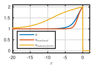
(a) $q=5$

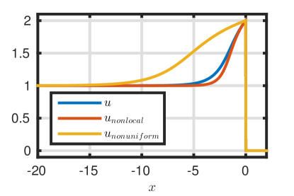
(b) $q=10$

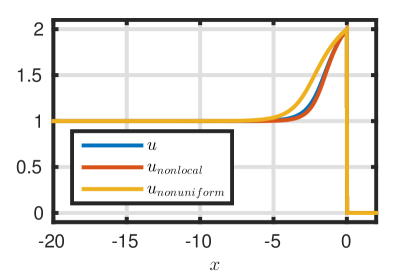
(c) $q=100$

Figure 2.1. Comparisons of the steady-state solutions for (2.6-2.9), using the temperatures: (i) $T=u/\sqrt{q}+\lambda$ (exact and local); (ii) $T=u_{s}/\sqrt{q}+\lambda$ (uniform and nonlocal approximation); and (iii) $T=\lambda$ (nonuniform approximation).

One difficulty with the procedure outlined in the previous paragraph for obtaining $f(x-x_{s},u_{s})$ from the reaction rate is that it may not be possible to integrate $\lambda_{x}=\omega\left(u_{s}\/,\,\lambda\right)$ analytically, and in a sufficiently simple form. In the physical example of an Arrhenius law, for instance, the equation to be integrated is

(2.11) $$\lambda_{x} = -k\hskip 1.00006pt(1-\lambda)\hskip 1.00006pt\exp\left(\theta q\left(\frac{u_{s}}{\sqrt{q}}+\lambda\right)\right).$$

This yields $\lambda$ implicitly, in terms of the inverse of an exponential integral. This inverse then needs to be differentiated in order to obtain $f(x-x_{s},u_{s})$, which produces a rather cumbersome expression. Because of these complications, when focusing on a specific example later in 4, we opt for simplicity and use an ad hoc explicit forcing function $f$ which captures the main qualitative features of simple chemical reactions.

3. Traveling wave solutions and stability analysis

In this section, we investigate the one-dimensional traveling wave solutions of (2.3-2.4), as well as their stability properties. Note that, since in the one-dimensional case the proposed system reduces to (LABEL:toy-model-1d), the traveling wave solutions are identical to those found in [5]. For completeness, we briefly repeat the discussion here.

3.1. Traveling wave solutions

We seek for solutions of (2.3-2.4) of the form $u(x,y,t)=u_{0}(x-Dt)$ and $v=0$ (more generally, $v$ constant) for $x\leq D\,t$, with $x_{s}=D\,t$ and $u_{s}=u_{s0}=u_{0}(0)$. It is easy to see that $u_{0}$ must have the form

(3.1) $$u_{0}(\xi) = D\pm\sqrt{C_{*}-2\int_{\xi}^{0}f\left(z,u_{0s}\right)\hskip 1.00006ptdz},$$

where $\xi=x-D\hskip 1.00006ptt$, and $C_{*}$ is an integration constant. The shock conditions at $x=x_{s}$, and the fact that the solution vanishes for $x>x_{s}$, yield $u_{s0}=2D>0$. This determines $C_{*}$ and the sign of the square root in (3.1). The full profile is then

(3.2) $$v\equiv 0\quad\mbox{and}\quad u(\xi)=\begin{cases}D+\sqrt{D^{2}-2\int_{\xi}^{0}f\left(z,u_{0s}\right)dz}&\text{for }\xi\leq 0,\\ 0&\text{for }\xi>0.\end{cases}$$

These are the traveling waves for the model; they consist of a shock of strength $2D>0$ moving into an unperturbed, unburnt state. For these solutions to be real, it must be that

(3.3) $$D=\zeta\hskip 1.00006pt\sqrt{2\int_{-\infty}^{0}f\left(y,u_{0s}\right)\hskip 1.00006ptdy},\quad\mbox{where}\;\;\zeta\geq 1.$$

The parameter $\zeta$ is the overdrive factor. The special value $\zeta=1$ corresponds to the slowest possible wave speed – the Chapman-Jouguet velocity. When $\zeta=1$, the characteristic speed (i.e., $u$) at the end of the reaction zone is equal to the wave speed $D$. On the other hand, waves with $\zeta>1$ are “overdriven”. For them, the characteristic speed is everywhere greater than the wave speed. Because of this, overdriven detonations are not self-sustained: the characteristics from any $\zeta<0$ catch up to the lead shock in a finite time, and affect its dynamics. Furthermore, the larger the overdrive, the closer the profile resembles that of an inert piston-induced shock. Therefore, in the limit of large overdrive, detonations are expected to be stable. We also point out here that, as in [5], the total energy release is assumed to be constant, i.e., $\int f\/dx=q/2=const$. As a result, $D$ is given explicitly by (3.3). Without this constraint on $f$, (3.3) would have been an implicit equation for $D$, because $u_{0s}=2D$.

Next we consider the multidimensional stability of the traveling waves given by (3.2).

3.2. Linear stability

We consider in this subsection the multi-dimensional linear stability for the solutions given by (3.2). For the purpose of the calculations that follow, it is convenient to rewrite (2.3-2.4) in a shock-attached frame. Assume that the shock position is given by a single valued function, $x_{s}=s(y\/,\,t)$, and introduce the shock-attached variable $\xi=x-s(y,t)$ to replace $x$. Then (2.3-2.4) takes the form

(3.4) $$u_{t}+(u-s_{t})\hskip 1.00006ptu_{\xi}+v_{y}-s_{y}\hskip 1.00006ptv_{\xi} = f(\xi,u_{s}),$$

(3.5) $$u_{y}-s_{y}\hskip 1.00006ptu_{\xi}-v_{\xi} = 0.$$

The quantities $s_{t}$ and $s_{y}$ are related to the states at the shock by the jump conditions, given by

(3.6) $$s_{t}\left[u\right]-\frac{1}{2}\left[u^{2}\right]+s_{y}\left[v\right] = 0,$$

(3.7) $$s_{y}\left[u\right]+\left[v\right] = 0,$$

where $[\cdot]$ represents the jump of a given quantity across the shock.

Next we expand $u=u_{0}(\xi)+\epsilon u_{1}(\xi,y,t)+O(\epsilon^{2})$, $v=\epsilon v_{1}(\xi,y,t)+O(\epsilon^{2})$, $s=Dt+\epsilon s_{1}(y,t)+O(\epsilon^{2})$, where $u_{0}$ is the steady profile, and $D=u_{0s}/2$ is the steady shock speed. Inserting these expressions into (3.4-3.5), and linearizing, we obtain

(3.8) $$u_{1t}+\left(u_{0}-\frac{u_{0s}}{2}\right)u_{1\xi}+u_{0}^{\prime}\hskip 1.00006ptu_{1}+v_{1y} =\left(\frac{\partial f}{\partial u_{s}}\left(x,u_{0s}\right)+\frac{1}{2}u_{0}^{\prime}\right)u_{1}\left(0,t\right),$$

(3.9) $$u_{1y}-u_{0}^{\prime}\hskip 1.00006pts_{1y}-v_{1\xi} =0,$$

where $u_{0}^{\prime}=\frac{d\/u_{0}}{d\/\xi}$, and the equations apply for $\xi\leq 0$ (the uniform state ahead of the shock is unperturbed). The linearized shock conditions are

(3.10) $$s_{1t}=\frac{1}{2}u_{1s}\quad\mbox{and}\quad s_{1y}=-\frac{v_{1s}}{u_{0s}},$$

where, as before, the subscript $s$ denotes evaluation at the post-shock state. It is convenient to introduce

$$c_{0}=u_{0}-\frac{1}{2}\hskip 1.00006ptu_{0s},\qquad b_{0}=\frac{\partial f}{\partial u_{s}}\left(x,u_{0s}\right)+\frac{1}{2}u_{0}^{\prime},$$

and then write (3.8-3.9) in the form

(3.11) $$u_{1t}+c_{0}\hskip 1.00006ptu_{1\xi}+u_{0}^{\prime}\hskip 1.00006ptu_{1}+v_{1y} =b_{0}\hskip 1.00006ptu_{1s},$$

(3.12) $$u_{1y}-v_{1\xi} =-u_{0\xi}\hskip 1.00006ptv_{1s}/u_{0s}.$$

Here $c_{0}$, $b_{0},$ and $u_{0s}$ are determined by the steady-state profile, while $u_{1s}=u_{1}(0,y,t)$ and $v_{1s}=v_{1}(0,y,t)$ denote the perturbed quantities evaluated immediately after the shock.

Linear instability (or stability) is determined by whether or not spatially bounded solutions to (3.11-3.12) that grow in time exist. In order to answer this question, we use transform methods, following the methodology in [3]. Because (3.11-3.12) has $y$-independent coefficients, we Fourier transform in the transverse direction:

(3.13) $$\hat{u}_{t}+c_{0}\hskip 1.00006pt\hat{u}_{\xi}+u_{0}^{\prime}\hskip 1.00006pt\hat{u}+i\hskip 1.00006pt\ell\hskip 1.00006pt\hat{v} = b_{0}\hskip 1.00006pt\hat{u}_{s},$$

(3.14) $$i\hskip 1.00006pt\ell\hskip 1.00006pt\hat{u}-\hat{v}_{\xi} = -\frac{u_{0}^{\prime}\hskip 1.00006pt\hat{v}_{s}}{u_{0s}},$$

where the parameter $\ell$ is the transverse wave number and

(3.15) $$\hat{u}(\xi,\ell,t) =\int_{-\infty}^{\infty}e^{-i\ell y}\hskip 1.00006ptu_{1}(\xi,y,t)\hskip 1.00006ptdy,\qquad\hat{u}_{s}(\ell,t)=\hat{u}(0,\ell,t),$$

(3.16) $$\hat{v}(\xi,\ell,t) =\int_{-\infty}^{\infty}e^{-i\ell y}\hskip 1.00006ptv_{1}(\xi,y,t)\hskip 1.00006ptdy,\qquad\hat{v}_{s}(\ell,t)=\hat{v}(0,\ell,t).$$

The Fourier transform of the linearized shock conditions in equation (3.10) is

(3.17) $$\hat{s}_{t}=\frac{1}{2}\,\hat{u}_{s}\quad\mbox{and}\quad i\hskip 1.00006pt\ell\hskip 1.00006ptu_{0s}\,\hat{s}=-\hat{v}_{s}\quad\mbox{where}\;\;\hat{s}(\ell,t)=\int_{-\infty}^{\infty}e^{-i\ell y}\hskip 1.00006pts_{1}(y,t)\hskip 1.00006ptdy.$$

Next, we Laplace transform in $t$ equations (3.13-3.14), and obtain

(3.18) $$\sigma\hskip 1.00006ptU-\hat{u}(\xi,\ell,0)+c_{0}\hskip 1.00006ptU_{\xi}+u_{0}^{\prime}\hskip 1.00006ptU+i\hskip 1.00006pt\ell\hskip 1.00006ptV = b_{0}\hskip 1.00006ptU_{s},$$

(3.19) $$i\hskip 1.00006pt\ell\hskip 1.00006ptU-V_{\xi} = -\frac{u_{0}^{\prime}\hskip 1.00006ptV_{s}}{u_{0s}},$$

where

(3.20) $$U(\xi,\ell,\sigma) =\int_{0}^{\infty}e^{-\sigma t}\hskip 1.00006pt\hat{u}(\xi,\ell,t)\hskip 1.00006ptdt,\qquad\mbox{with}\;\;U_{s}(\ell,\sigma)=U(0,\ell,\sigma),$$

(3.21) $$V(\xi,\ell,\sigma) =\int_{0}^{\infty}e^{-\sigma t}\hskip 1.00006pt\hat{v}(\xi,\ell,t)\hskip 1.00006ptdt,\qquad\mbox{with}\;\;V_{s}(\ell,\sigma)=V(0,\ell,\sigma).$$

Note 1.

The issue of stability/instability reduces now to the question of the (possible) existence of singularities in the Laplace Transform for $\Re(\sigma)>0$. Thus we take $\Re(\sigma)>0$ in what follows. For that matter: we can calculate assuming $\sigma$ real, large, and positive; and then extend the result by analytic continuation.  $\clubsuit\/$

Now rewrite (3.18-3.19) in matrix form

(3.22) $$\mathbf{A}\cdot\frac{d}{d\xi}\mathbf{W}=\mathbf{B}\cdot\mathbf{W}+\mathbf{\tilde{F}}(\xi;\sigma,\ell),$$

where

(3.23) $$\mathbf{W}=\begin{bmatrix}U\\ V\end{bmatrix},\quad\mathbf{A}=\begin{bmatrix}c_{0}&0\\ 0&1\end{bmatrix},\quad\mathbf{B}=\begin{bmatrix}-\sigma-u_{0}^{\prime}&-i\hskip 1.00006pt\ell\\ i\hskip 1.00006pt\ell&0\end{bmatrix},\quad\mbox{and}\quad\mathbf{\tilde{F}}=\begin{bmatrix}\hat{u}(\xi,\ell,0)+b_{0}\hskip 1.00006ptU_{s}\\ u_{0}^{\prime}\hskip 1.00006ptV_{s}/u_{0s}\end{bmatrix}.$$

Two cases arise now, which are different in terms of their analytic complexity.

The first case is the overdriven detonation, where $\zeta>1$ in (LABEL:u0s). In this case $c_{0}>0$ for all $\xi<0$. Thus no sonic point exists in the steady state, $\mathbf{A}$ is invertible everywhere, and (3.22) is equivalent to

(3.24) $$\frac{d}{d\xi}\mathbf{W}=\mathbf{C}\cdot\mathbf{W}+\mathbf{F}(\xi;\sigma,\ell),$$

where

$$\mathbf{C}=\mathbf{A}^{-1}\hskip 1.00006pt\mathbf{B}=\begin{bmatrix}\left(-\sigma-u_{0}^{\prime}\right)/c_{0}&-i\hskip 1.00006pt\ell/c_{0}\\ i\hskip 1.00006pt\ell&0\end{bmatrix}\;\;\mbox{and}\;\;\mathbf{F}=\mathbf{A}^{-1}\hskip 1.00006pt\mathbf{\tilde{F}}=\begin{bmatrix}\left(\hat{u}(\xi,\ell,0)+b_{0}\hskip 1.00006ptU_{s}\right)/c_{0}\\ u_{0}^{\prime}\hskip 1.00006ptV_{s}/u_{0s}\end{bmatrix}.$$

Here, due to the overdrive assumption, $\mathbf{C}$ is a bounded matrix.

The second (harder) case is the Chapman-Jouguet detonation, wherein $c_{0}(\xi)\to 0$ as $\xi\to-\infty$.   Then, $\mathbf{A}$ is no longer invertible at the sonic point. Hence, a necessary condition for $\frac{d}{d\xi}\mathbf{W}$ to remain bounded as $\xi\rightarrow-\infty$ is that the right hand side of (3.22) become orthogonal to the left eigenvector corresponding to the vanishing eigenvalue of $\mathbf{A}$, i.e.,

$$\lim_{\xi\to-\infty}\mathbf{l}_{i}\cdot\mathbf{A}\hskip 1.00006pt\frac{d}{d\xi}\mathbf{W} =\lim_{\xi\to-\infty}\lambda_{i}\hskip 1.00006pt\mathbf{l}_{i}\cdot\frac{d}{d\xi}\mathbf{W}$$

$$=\lim_{\xi\to-\infty}\mathbf{l}_{i}\cdot\left(\mathbf{B}\cdot\mathbf{W}+\mathbf{\tilde{F}}(\xi;\sigma,\ell)\right)=0,$$

where $\lambda_{i}$ is the eigenvalue that vanishes as $\xi\to-\infty$, and $\mathbf{l}_{i}$ is the corresponding eigenvector. Given the form of $\mathbf{A}$, $\mathbf{B}$, and $\mathbf{F}$, this is equivalent to

(3.25) $$\left(\sigma+u_{0}^{\prime}(\xi)\right)\hskip 1.00006ptU+i\hskip 1.00006pt\ell\hskip 1.00006ptV\rightarrow 0\qquad\text{as}\qquad\xi\to-\infty.$$

This last equation is called the radiation, or boundedness, condition. To avoid the difficulties related to the vanishing of $c_{0}$, for the remainder of this paper we focus on overdriven detonations.

Using a fundamental matrix for the homogeneous problem [1], we can write the solution to (LABEL:overdriven-ode-laplace-matrix) in terms of the boundary data at $\xi=0$, and the initial data (encoded into $\mathbf{F}$). That is,

(3.26) $$\mathbf{W}(\xi;\sigma,\ell)=\mathbf{H}(x;\sigma,\ell)\cdot\left[\mathbf{H}^{-1}(0;\sigma,\ell)\cdot\mathbf{W}(0;\sigma,\ell)+\int_{0}^{x}\mathbf{H}^{-1}(z;\sigma,\ell)\cdot\mathbf{F}(z;\sigma,\ell)\hskip 1.00006ptdz\right],$$

where $\mathbf{H}$ is a non-singular matrix solution of the homogeneous problem: $\frac{d}{d\xi}\hskip 1.00006pt\mathbf{H}=\mathbf{C}\cdot\mathbf{H}$ with det$(\mathbf{H})\neq 0$. We denote the columns of $\mathbf{H}$ by $\mathbf{h}_{1}$ and $\mathbf{h}_{2}$, so that $\mathbf{H}=[\mathbf{h}_{1},\mathbf{h}_{2}]$.

Define $\delta=\lim_{\xi\rightarrow-\infty}\hskip 1.00006ptc_{0}(\xi)>0$ and

(3.27) $$\mathbf{C}_{-\infty}=\lim_{\xi\to-\infty}\mathbf{C}(\xi)=\begin{bmatrix}-\sigma/\delta&-i\hskip 1.00006pt\ell/\delta\\ i\hskip 1.00006pt\ell&0\end{bmatrix}.$$

$\mathbf{C_{\infty}}$ is a constant matrix with (generally distinct) eigenvalues

(3.28) $$\lambda_{1}=\frac{-\sigma-\sqrt{4\hskip 1.00006pt\delta\hskip 1.00006pt\ell^{2}+\sigma^{2}}}{2\hskip 1.00006pt\delta}\quad\mbox{and}\quad\lambda_{2}=\frac{-\sigma+\sqrt{4\hskip 1.00006pt\delta\hskip 1.00006pt\ell^{2}+\sigma^{2}}}{2\hskip 1.00006pt\delta},$$

where we use the principal branch for the square root. Let $\mathbf{q}_{1}$ and $\mathbf{q}_{2}$ be the corresponding eigenvectors. Then, provided that the limit in (3.27) is achieved “fast enough”, $\mathbf{h}_{1}$ and $\mathbf{h}_{2}$ can be selected so that (see Appendix A)

(3.29) $$\mathbf{h}_{1}\sim e^{\lambda_{1}\hskip 0.70004pt\xi}\hskip 1.00006pt\mathbf{q}_{1}\quad\mbox{and}\quad\mathbf{h}_{2}\sim e^{\lambda_{2}\hskip 0.70004pt\xi}\hskip 1.00006pt\mathbf{q}_{2}\quad\mbox{as }\;\xi\to-\infty.$$

Since $\Re(\lambda_{1})<0<\Re(\lambda_{2})$, $\mathbf{h}_{1}$ grows exponentially as $\xi\to-\infty$, while $\mathbf{h}_{2}$ decays. Let now $\boldsymbol{\theta}_{1}$ and $\boldsymbol{\theta}_{2}$ be the rows of $\mathbf{H}^{-1}$. Then

(3.30) $$\boldsymbol{\theta}_{j}\sim e^{-\lambda_{j}\hskip 0.70004pt\xi}\boldsymbol{\pi}_{j}\quad\mbox{as }\;\xi\to-\infty,$$

where the $\boldsymbol{\pi}_{j}$ are constant vectors. Furthermore, the $h_{j}$ and $\theta_{j}$ have analytic dependence on $\sigma$, for $\Re(\sigma)>0$ (Appendix A).

With the notation above the solution to (3.24) can now be written in the form

(3.31) $$\mathbf{W}(\xi)=\left(\boldsymbol{\theta}_{1}(0)\cdot\mathbf{W}(0)+\int_{0}^{\xi}\boldsymbol{\theta}_{1}(z)\cdot\mathbf{F}(s)\hskip 1.00006ptds\right)\mathbf{h}_{1}+\left(\boldsymbol{\theta}_{2}(0)\cdot\mathbf{W}(0)+\int_{0}^{\xi}\boldsymbol{\theta}_{2}(z)\cdot\mathbf{F}(s)\hskip 1.00006ptds\right)\mathbf{h}_{2},$$

where we only display the dependence on $\xi$. Further, boundedness of $\mathbf{W}(\xi)$ as $\xi\rightarrow-\infty$ requires a choice which eliminates the exponentially growing part of the solution. Specifically:

(3.32) $$\boldsymbol{\theta}_{1}(0)\cdot\mathbf{W}(0)=\lim_{x\rightarrow-\infty}\hskip 1.00006pt\int_{x}^{0}\boldsymbol{\theta}_{1}(z)\cdot\mathbf{F}(z)\hskip 1.00006ptdz.$$

That this choice is also sufficient to guarantee a bounded solution is less obvious, but a proof (given in the context of the reactive Euler equations) can be found in [3]. Inserting back the definition of $\mathbf{F}$, we obtain

(3.33) $$\boldsymbol{\theta}_{1}(0)\cdot\mathbf{W}(0)=\int_{-\infty}^{0}\boldsymbol{\theta}_{1}\cdot\begin{bmatrix}\left(\hat{u}(\xi,\ell,0)+b_{0}\hskip 1.00006ptU_{s}\right)/c_{0}\\ u_{0}^{\prime}\hskip 1.00006ptV_{s}/u_{0s}\end{bmatrix}dz.$$

The Laplace transform of the linearized jump conditions (3.17) can be used to relate $V_{s}$ to $U_{s}$ via

(3.34) $$\sigma\hskip 1.00006ptV_{s}=-i\hskip 1.00006pt\ell\hskip 1.00006ptu_{0s}\left(\frac{1}{2}\hskip 1.00006ptU_{s}+\hat{s}(\ell,0)\right).$$

Since neither the $h_{j}$, nor the $\theta_{j}$ have singular dependence on $\sigma$, equation (3.31) shows that singular dependence can enter only through the boundary data at $\xi=0$, that is: $U_{s}$ and $V_{s}$. From (3.34) it then follows that the stability/instability issue, see Note 1, can be decided solely by inspecting the (possible) singularities in $U_{s}=U|_{\xi=0}$. To this end, insert now (3.34) into (3.33), and solve for $U_{s}$. This yields

(3.35) $$U_{s}=\frac{\;\boldsymbol{\theta}_{1}(0)\cdot\begin{bmatrix}0\\ i\hskip 1.00006pt\ell\hskip 1.00006ptu_{0s}\hskip 1.00006pt\hat{s}(\ell,0)\end{bmatrix}+\sigma\int_{-\infty}^{0}\boldsymbol{\theta}_{1}\cdot\begin{bmatrix}\hat{u}(\xi,\ell,0)/c_{0}\\ i\hskip 1.00006pt\ell\hskip 1.00006ptu_{0}^{\prime}\hskip 1.00006pt\hat{s}(\ell,0)\end{bmatrix}\hskip 1.00006ptdz\;}{\boldsymbol{\theta}_{1}(0)\cdot\begin{bmatrix}\sigma\\ -\frac{1}{2}\hskip 1.00006pti\hskip 1.00006pt\ell\hskip 1.00006ptu_{0s}\end{bmatrix}-\int_{-\infty}^{0}\boldsymbol{\theta}_{1}\cdot\begin{bmatrix}\sigma\hskip 1.00006ptb_{0}/c_{0}\\ \frac{1}{2}\hskip 1.00006pti\ell\hskip 1.00006ptu_{0}^{\prime}\end{bmatrix}\hskip 1.00006ptdz}.$$

Because $\boldsymbol{\theta}_{1}$ decays exponentially as $\xi\to-\infty$, here both the numerator and denominator are regular functions of $\sigma$ for $\Re(\sigma)>0$. The possible singularities are thus poles (denominator roots), i.e., solutions to

(3.36) $$\boldsymbol{\theta}_{1}(0)\cdot\begin{bmatrix}\sigma\\ -\frac{1}{2}\hskip 1.00006pti\hskip 1.00006pt\ell\end{bmatrix}=\int_{-\infty}^{0}\boldsymbol{\theta}_{1}\cdot\begin{bmatrix}\sigma\hskip 1.00006ptb_{0}/c_{0}\\ \frac{1}{2}\hskip 1.00006pti\hskip 1.00006pt\ell\hskip 1.00006ptu_{0}^{\prime}\end{bmatrix}\hskip 1.00006ptdz.$$

The function $\boldsymbol{\theta}_{1}$ solves the adjoint homogeneous problem

$$\frac{d}{d\xi}\boldsymbol{\theta} = -\mathbf{C}(\xi;\sigma,\ell)^{T}\cdot\boldsymbol{\theta},$$

$$= \begin{bmatrix}\left(\sigma+u_{0}^{\prime}\right)/c_{0}&-i\hskip 1.00006pt\ell\\ i\hskip 1.00006pt\ell/c_{0}&0\end{bmatrix}\boldsymbol{\theta},$$

subject to the condition that $\boldsymbol{\theta}$ should be bounded as $\xi\to-\infty$. Thus in this limit $\boldsymbol{\theta}_{1}$ becomes parallel to the eigenvector associated to the eigenvalue with positive real part:

(3.38) $$\boldsymbol{\theta}_{1}\sim a\hskip 1.00006pt\begin{bmatrix}\frac{1}{2}\,\left(\sigma+\sqrt{4\hskip 1.00006pt\ell^{2}\hskip 1.00006pt\delta+\sigma^{2}}\right)\\ i\hskip 1.00006pt\ell\end{bmatrix}\hskip 1.00006pte^{-\lambda_{1}\hskip 0.70004pt\xi}\quad\mbox{as}\;\;\xi\to-\infty,$$

where $a\neq 0$ is a constant. Note that the value of $a$ has no effect on equation (3.36).

When $\ell=0$, the adjoint homogeneous problem (3.2) becomes the scalar equation

(3.39) $$\frac{d}{d\xi}\mathbf{\theta}=\frac{1}{c_{0}}\hskip 1.00006pt\left(\sigma+u_{0}^{\prime}\right)\hskip 1.00006pt\mathbf{\theta},$$

with solutions

(3.40) $$\mathbf{\theta}=\frac{\theta(0)}{c_{0}(0)}\hskip 1.00006ptc_{0}(\xi)\hskip 1.00006pt\exp(-\sigma\hskip 1.00006ptp(\xi)),\quad\mbox{where}\;\;p=\int_{\xi}^{0}\frac{1}{c_{0}}\hskip 1.00006ptdz.$$

Using (3.40) in (3.36) yields

(3.41) $$c_{0}(0)=\int_{-\infty}^{0}b_{0}(z)\hskip 1.00006pte^{-\sigma\hskip 0.70004ptp(z)}\hskip 1.00006ptdz$$

as the equation for the poles of the Laplace Transform in $\Re(\sigma)>0$. This is the same as the dispersion relation obtained in [5], using a normal mode approach. It follows that, in the context of the simple toy model presented here:

1. The Laplace transform and normal mode approaches yield the same stability criterion in 1D.

2. The difficulties with the stability analysis for a Chapman-Jouguet detonation, see equation (3.25), do not arise in 1D (i.e., $\ell=0$) for the analog model. The reason is that, in this case, the linearized equations can be solved (essentially) explicitly. This analysis, using normal modes, can be found in [5] as well. Surprisingly, the answer is the same as for overdriven detonations; i.e., the stability criterion is also (3.41). Thus the question, requiring further investigation is: is this still true when $\ell\neq 0$?

In general, for $\ell\neq 0$, (LABEL:adjoint-homogenous-problem) cannot be solved analytically. Then a numerical method is needed to obtain the eigenvalues (poles of the Laplace transform), given by the roots $\sigma=\sigma(\ell)$ of

(3.42) $$0=R(\sigma,\ell)=\boldsymbol{\theta}_{1}(0)\cdot\begin{bmatrix}\sigma\\ -\frac{1}{2}\hskip 1.00006pti\hskip 1.00006pt\ell\end{bmatrix}-\int_{-\infty}^{0}\boldsymbol{\theta}_{1}\cdot\begin{bmatrix}\sigma\hskip 1.00006ptb_{0}/c_{0}\\ \frac{1}{2}\hskip 1.00006pti\hskip 1.00006pt\ell\hskip 1.00006ptu_{0}^{\prime}\end{bmatrix}\hskip 1.00006ptdz,$$

where $\boldsymbol{\theta}_{1}$ is as in (3.2-3.38).

4. An example

In this section, we select a specific form for the forcing function $f$, and use it to illustrate particular properties of the model. For this purpose, we could use the more physically justifiable reaction rate that follows from the approach in (2.10-2.11). However, as pointed out earlier, this gives rise to certain complications because we cannot solve (2.11) for $\lambda$ explicitly, which leads to a forcing function that is both costly to compute numerically, and hard to understand analytically. We therefore diverge here from a rational approach and aim instead at simplicity, choosing $f$ in an ad hoc manner.

Motivated by the one dimensional analog model presented in [13, 5], we choose $f$ to have the form

$$f=\frac{q}{\sqrt{4\hskip 1.00006pt\pi\hskip 1.00006pt\beta}\left(1+\text{Erf}\left[\frac{k}{2\,\sqrt{\beta}}\,\left(\frac{u_{s}}{u_{0s}}\right)^{-\alpha}\right]\right)}\hskip 1.00006pt\exp\left[-\frac{1}{4\,\beta}\hskip 1.00006pt\left(x-x_{s}+k\hskip 1.00006pt\left(\frac{u_{0s}}{u_{s}}\right)^{\alpha}\right)^{2}\right]$$

for $x<x_{s}$, where $q>0$, $k>0$, $\beta>0$, and $\alpha>0$ are parameters, and $f=0$ ahead of the shock, $x>x_{s}$.

The form above mimics important features of the reaction rate, controlled by the parameters. It has an induction length (determined by $k$), a reaction-zone width (governed by $\beta$), and a heat release $q$ (note that the total energy release is constant, $\int f\/dx=q/2$, as in [5]). Finally, $\alpha$ regulates the sensitivity to the shock velocity (and plays a role similar to that of the activation energy).

It is convenient to rescale the variables as follows

$$u=u_{0s}\hskip 1.00006pt\tilde{u},\quad v=u_{0s}^{3/2}\hskip 1.00006pt\tilde{v},\quad x=k\hskip 1.00006pt\tilde{x},\quad y=k\hskip 1.00006pt\tilde{y}/\sqrt{u_{0s}},\quad t=k\hskip 1.00006pt\tilde{t}/u_{0s},$$

where $u_{0s}$ is given by (LABEL:u0s). Then the model equations take the form

(4.1) $$\tilde{u}_{\tilde{t}}+\frac{1}{2}\left(\tilde{u}^{2}\right)_{\tilde{x}}+\tilde{v}_{\tilde{y}} = \tilde{f}(\tilde{x}-\tilde{x}_{s},\tilde{u}_{s}),$$

(4.2) $$\tilde{v}_{\tilde{x}}-\tilde{u}_{\tilde{y}} = 0,$$

where the rescaled forcing function $\tilde{f}$ is

(4.3) $$\tilde{f}(\tilde{x}-\tilde{x}_{s},\tilde{u_{s}})=\frac{1}{4\zeta^{2}\left(1+\text{Erf}\left[\frac{\tilde{u}(0,\tilde{t})^{-\alpha}}{2\sqrt{\tilde{\beta}}}\right]\right)}\frac{1}{\sqrt{4\hskip 1.00006pt\pi\hskip 1.00006pt\tilde{\beta}}}\hskip 1.00006pt\exp\left[-\frac{1}{4\hskip 1.00006pt\tilde{\beta}}\hskip 1.00006pt\left(\tilde{x}-\tilde{x}_{s}+\left(\tilde{u}\left(0,\tilde{t}\right)\right)^{-\alpha}\right)^{2}\right],$$

$\tilde{\beta}=\beta/k$, and $\zeta$ is the overdrive parameter introduced in (3.3).

Therefore, the wave dynamics is controlled by three parameters: $\alpha$ – sensitivity of the reaction rate to variations in $u$ at the shock, $\tilde{\beta}$ – ratio of the reaction zone length to the induction zone length, and $\zeta$ – the degree of overdrive. From here on we use the dimensionless variables, and drop the tilde notation.

In the dimensionless equations, the overdrive $\zeta$ scales the amplitude of the source term. Thus, the influence of chemical reactions vanishes as $\zeta\to\infty$, and the wave approaches an inert shock. This is illustrated by 4.1, showing the effect of the overdrive factor on the steady detonation profile. For large enough overdrive, $u$ becomes nearly constant behind the precursor shock, and the wave is primarily sustained by the imposed left boundary condition.

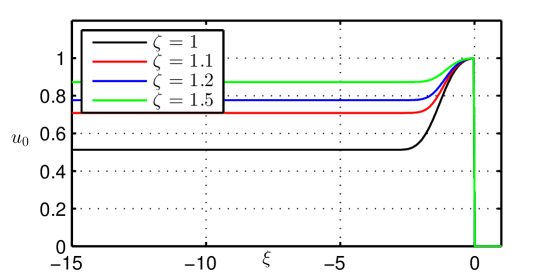
Figure 4.1. Steady-state solution profiles for (2.3-2.4) as the overdrive is varied, while keeping all other parameters fixed.

In the next subsection we focus on the role played by multi-dimensional effects on: (1) the linear stability properties, and (2) the full nonlinear dynamics of the solutions to (4.1-4.2). The goal is to show that multi-dimensional instabilities typically dominate one-dimensional instabilities, and that these instabilities lead to the formation of complex patterns in the solutions to (4.1-4.2). We start with the linear stability analysis.

4.1. Multidimensional linear stability analysis

As shown in Section 3.2, the stability question for the steady state solutions of (4.1-4.2) is decided by the roots of the stability function $R(\sigma\/,\,\ell)$, defined in (3.42). If zeros exist with $\Re(\sigma)>0$ for any admissible $\ell$ (discrete or continuous depending on whether the domain in $y$ is bounded or not), then the profile is unstable. Otherwise, it is stable. The main difficulty with finding the roots to (3.42) stems from the fact that $\theta_{1}$, defined in (3.2-3.38), must be computed numerically. Thus, each evaluation of $R(\sigma,\ell)$ requires solving the linear ODE system (3.2) to obtain $\theta_{1}$, followed by a numerical evaluation of the integral in the definition of $R$. This makes parametric studies for varying $\alpha$ and $\beta$ computationally costly. We start by investigating the overdrive effect on the wave stability. As pointed out earlier, because detonations become “closer” to inert shocks the larger the overdrive is, we expect the overdrive to have a stabilizing effect. This is confirmed by 4.2(a), where the growth rate $\sigma_{r}=\Re(\sigma(\ell))$, as a function of the transverse wave number $\ell$, for $\beta=0.1$ and $\alpha=4.05$, is plotted for increasing values of the overdrive parameter $\zeta=1.05$, $1.10$, and $1.20$. For the calculations in this subsection, it turns out that equation (3.42) has a single root in $\Re(\sigma)>0$. In general, the growth rate is the maximum value over all the roots of $\Re(\sigma)$. It is seen in 4.2(a) that the maximum growth rate occurs at a value $\ell\neq 0$. In particular, waves that are stable to purely longitudinal disturbances $\left(\ell=0\right)$, can be unstable to 2D perturbations. Thus, generally, we expect multi-dimensional effects to dominate over 1D effects.

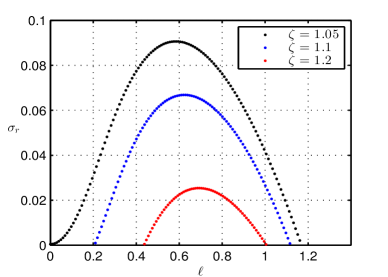
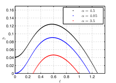
Figure 4.2. Growth rate, $\sigma_{r}$, as a function of the transverse wavenumber, $l$ : (a) at $\beta=0.1$, $\alpha=4.05$, and varying degree of overdrive, $\zeta$; (b) at $\beta=0.1$, $\zeta=1.05$, and varying $\alpha$.

We also study the effect of $\alpha$ on the stability of the waves. Since $\alpha$ measures the sensitivity of the forcing to changes in the lead shock strength, we expect that larger values of $\alpha$ will augment the instability. Specifically, the growth rate $\sigma_{r}$ should increase with $\alpha$. This is precisely what is observed in 4.2(b). This figure also shows that $\alpha$ seems to have very little effect on the value of $\ell$ corresponding to the most unstable transverse mode. In particular, for the parameters in 4.2(b), the most unstable mode occurs for $\ell\approx 0.6$, regardless of the value $\alpha$ takes. This behavior is similar to the observation in [5] for the 1D stability. That is, $\alpha$ has very little effect on the imaginary part of the unstable eigenvalues (recall that [5] uses a mode based stability analysis).

4.2. Numerical simulations

The linear stability results presented in § 4.1 suggest that 2D effects play an important role in the solutions of (4.1-4.2). Here, we investigate what happens after the onset of the instabilities. We use numerical simulations to investigate the large time limit of solutions to (2.3-2.4), which start from initial conditions given by (linearly unstable) ZND profiles (3.1). These calculations show that the two-dimensional analog model exhibits many of the interesting features of real multi-dimensional detonations.

The numerical simulation of (2.3-2.4) poses some problems. On the one hand, because it is a genuinely nonlinear hyperbolic system, shocks can form even when starting from smooth initial data. On the other hand, it has characteristic surfaces which are orthogonal to time. Thus the evolution in time is a nonlocal process. A scheme capable of dealing with shocks is needed, but it cannot be fully explicit since it is impossible to satisfy a typical CFL condition. Even with no reaction, $f\equiv 0$, when the equations reduce to

(4.4) $$u_{t}+\left(\frac{1}{2}\,u^{2}\right)_{x}+v_{y} = 0,$$

(4.5) $$v_{x}-u_{y} = 0,$$

developing an appropriate algorithm is not straightforward (e.g., see [11, 23]). We solve (2.3-2.4) using an algorithm based on a semi-implicit time discretization. The approach is discussed in [6], where a detailed numerical study of asymptotic equations similar to (2.3-2.4) is performed. Finally, we note that using a shock-fitting algorithm is not as simple as in the one-dimensional case [5], due to the presence of transverse shocks. We therefore adopt a shock capturing approach. Equations (2.3-2.4) are solved in an inertial frame of reference moving with constant speed $D=1/2$, which is the speed of the unperturbed ZND wave. The top and bottom ($y$ coordinate) boundary conditions are that of a rigid wall. An inflow boundary condition on the right, and an outflow on the left are given. We have verified that, when linear stability predicts a stable traveling wave (e.g., when $\alpha$ is small enough), the numerical solver is able to correctly capture the ZND structure and wave speed, even when a small amplitude perturbation is initially imposed on the exact ZND profile. Interesting dynamics are observed for parameters selected so that the initial data is unstable. If the ZND wave is only weakly unstable (meaning the parameters are close to the neutral stability boundary), very regular multi-dimensional patterns are observed: see 4.3. Figure 4.3(b) displays regions where the induction zone length (distance between the lead shock and the peak of $f$) is significantly reduced relative to the ZND theory. In these regions the energy is released shortly after the lead shock. The associated transverse waves, however, appear to be smooth: 4.3(a).

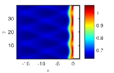
(a) $u$ at time $t=800$.

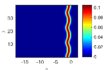
(b) $f$ at time $t=800$.

Figure 4.3. Large time dynamics for $\beta=0.1$, $\alpha=3.5$, and $\zeta=1.05$. This corresponds to a weakly unstable regime, with regular structures forming, and small transverse velocities.

Next, we investigate the effect of the overdrive parameter $\zeta$. Waves closer to the Chapman-Jouguet case are more unstable and display stronger transverse variations. Furthermore, for smaller overdrives, the cells in the patterns are larger. These findings are consistent with the linear stability prediction in 4.2. There it can be seen that: (1) smaller $\zeta$ corresponds to larger growth rates, and (2) the most unstable wavelength increases with decreasing degree of overdrive. Figure 4.4 illustrates these points.

(a) $u$ at $t=1000$, for $\zeta=1.10$.

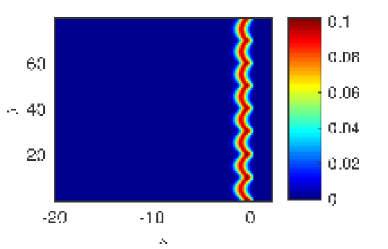
(b) $f$ at $t=1000$, for $\zeta=1.10$.

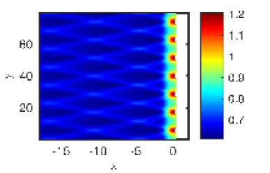
(c) $u$ at $t=1000$, for $\zeta=1.05$.

(d) $f$ at $t=1000$, for $\zeta=1.05$.

Figure 4.4. Cellular patterns at varying overdrive, $\zeta$, and $\alpha=4.05$, $\beta=0.1$.

Figure 4.5 explores the effect of $\alpha$, the shock-state sensitivity of the reaction rate, on the detonation wave structure and stability. As in the one dimensional case [5], larger values of $\alpha$ are associated with more complex dynamics. As $\alpha$ grows, so does the strength of the patterns generated, which also become more irregular. Figure 4.5(e-f) shows an example of an irregular cellular detonation wave.

(a) $u$ at $t=1000$, for $\alpha=4.05$.

(b) $f$ at $t=1000$, for $\alpha=4.05$.

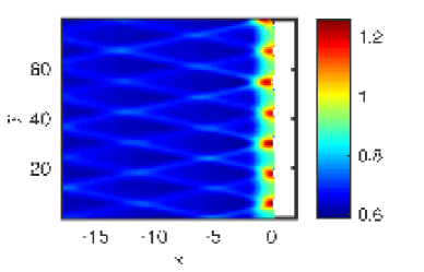
(c) $u$ at $t=1000$, for $\alpha=4.30$.

(d) $f$ at $t=1000$, for $\alpha=4.30$.

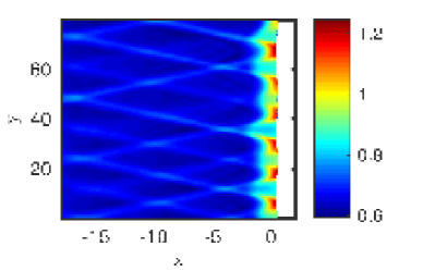
(e) $u$ at $t=1000$, for $\alpha=4.50$.

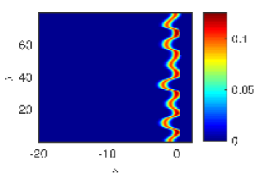
(f) $f$ at $t=1000$, for $\alpha=4.50$.

Figure 4.5. Large time behavior of the solutions for $\zeta=1.05$, $\beta=0.1$, and varying $\alpha$.

These figures, qualitatively, match well the cellular patterns observed for gaseous detonations in dilute mixtures [14, 9, 18]. However, a quantitative characterization of the two-dimensional dynamics, of the sort found for the 1D case in [5], is challenging. As $\alpha$ increases, the solutions are seen to go through a series of bifurcations, and transition: from (i) a very regular, periodic, structure; to (iii) irregular and aperiodic behavior; through (ii) intermediate stages of increasing complexity. These stages are illustrated by each of the rows in 4.5. Panels (a-b) correspond to a very simple, periodic, structure. Panels (c-d) show some extra structure, easily detectable in the $y$-direction in panel (d). Finally, the waves in panels (e-f) are fairly irregular.

Figures 4.6 through 4.8 display the time history of the gradient of $v$, for successively higher values of $\alpha$. These plots are produced as follows. First, we convert the solutions from the ZND-wave moving frame (used for the numerical calculation) back to the “lab” frame $(x_{l}\/,\,y_{l})$. The calculation is run for a long enough time, $0\leq t\leq T_{f}$, to insure that transient effects are gone. This results into the lead shock moving (in the lab frame) several hundred units: the shock starts at $x_{l}\approx 20$, and it is beyond $x_{l}=400$ by $t=T_{f}$. Second, we construct the “trace” of $|\nabla v|$, using the formula

(4.6) $$Tr(x_{l}\/,\,y_{l})=\int_{0}^{T_{f}}|\nabla v(x_{l}\/,\,y_{l}\/,\,t)|\hskip 1.00006ptdt.$$

This formula makes sense even if $v$ is discontinuous, and is equivalent to the total variation in time at a given point $(x_{l},y_{l})$. The trace is then plotted for $x_{l}$ in the interval $0\leq x_{l}\leq 360$. The results are displayed in figures 4.6-4.8. Note that, since the transverse waves are stronger closer to the lead shock (and decay away from it), moving left to right in these plots is (roughly) equivalent to exploring the evolution in time of the transverse waves. The process described above is a numerical analog of the experimental soot foil records of detonations. A related approach was used in [19], where the authors traced the time integral of a specific energy release at a given location.

The plots illustrate that the regularity of the final cellular structure produced depends on the distance to the stability boundary (larger the larger $\alpha$ is), as well as several other properties. For $\alpha=4.1$, 4.6 shows that the cells become regular after a sufficiently long time. Initially (top panel), cells of differing strengths coexist, and there is some irregularity in the pattern. After a while, the pattern becomes nearly regular, with only a low frequency modulation remaining. This is apparent in the middle panel, which exhibits slight horizontal waviness (easier to see along the whitest regions of the plot). This transient decays slowly, and eventually disappears — the bottom panel shows very little of it.

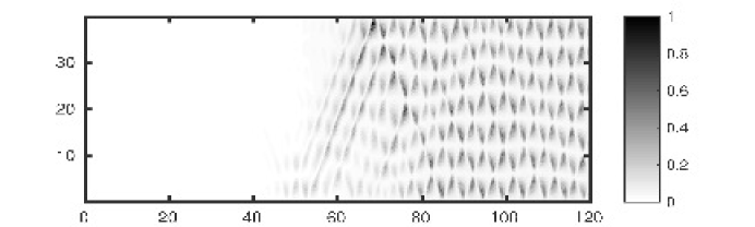
(a)

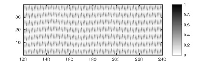
(b)

(c)

Figure 4.6. Trace of $|\nabla v|$, as in (LABEL:tracegradv), for $\alpha=4.1$, with $\beta=0.1$ and $\zeta=1.05$. The horizontal and vertical plot axes are $x_{l}$ and $y_{l}$, and the intensity gray bar is normalized to $[0\/,\,1]$. Each panel corresponds to a third of the plot range $0\leq x_{l}\leq 360$.

Figure 4.7, corresponding to $\alpha=4.5$, exhibits an interesting phenomenon. Initially (top panel), the cells are relatively small. However, after a while, cells that are about twice as large as the original ones appear (middle panel), while the smaller ones gradually decay. Eventually (bottom panel), the larger cells completely take over the pattern. This behavior is similar to the one found in detonation simulations with the reactive Euler equations. That is: the initial cell sizes are found to be consistent with the length scale provided by the most unstable linear mode, but the long time behavior is dominated by cells that can be significantly larger [10, 22]. In fact, to further stress this point, note that: in each of the figures the initial cell size is, roughly, the same. This corresponds to the fact that $\ell$ for the most unstable linear mode does not change much when $\alpha$ changes — see figure 4.2. On the other hand, the onset of the cells happens earlier as $\alpha$ grows, because the growth rate of the most unstable linear mode also increases with $\alpha$.

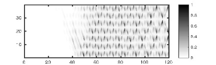
(a)

(b)

(c)

Figure 4.7. Trace of $|\nabla v|$, as in (LABEL:tracegradv), for $\alpha=4.5$, with $\beta=0.1$ and $\zeta=1.05$. The horizontal and vertical plot axes are $x_{l}$ and $y_{l}$, and the intensity gray bar is normalized to $[0\/,\,1]$. Each panel corresponds to a third of the plot range $0\leq x_{l}\leq 360$. The dashed line in panel (c) tracks a transverse wave as it bounces back-and-forth from the boundaries.

When $\alpha$ is increased further, as in 4.8, cell regularity is lost (at least for the time scales our computations explored). Here, again, the average cell size increases after the initial transient stage.

(a)

(b)

(c)

Figure 4.8. Trace of $|\nabla v|$, as in (LABEL:tracegradv), for $\alpha=4.8$, with $\beta=0.1$ and $\zeta=1.05$. The horizontal and vertical plot axes are $x_{l}$ and $y_{l}$, and the intensity gray bar is normalized to $[0\/,\,1]$. Each panel corresponds to a third of the plot range $0\leq x_{l}\leq 360$.

Another peculiar feature, which can be seen in 4.7, is that the amplitude of the transverse waves has large variations as they bounce back-and-forth from the channel walls. This can be verified by tracing the path of any single wave as it bounces from the walls (see the dashed line in the third panel of figure 4.7). It is possible that this is simply another transient phenomenon, decaying after a very long time. However, this may be a part of the multi-modal dynamics of the wave, being produced by the collisions between transverse waves and/or the interaction of the longitudinal and transverse instabilities, which are both present in this particular case.

5. Conclusions

A simple two-dimensional analog model for detonations was introduced. The model consists of a non-locally forced Burgers-like equation, coupled with a zero-vorticity equation, and extends our earlier model for one-dimensional pulsating detonations. The model was shown to be capable of capturing the multi-dimensional principal characteristics of cellular detonations, wherein transverse shocks and associated triple-point formation play an important role.

A Laplace transform approach was employed to perform a linear stability analysis of the model traveling wave solutions. It was shown that the dispersion relation for the unstable modes can be written as an integral equation, much like the explicit 1D result derived in [5]. However, in 2D evaluation of the dispersion relation requires a computationally intensive procedure, as it is also the case for detonations modeled by the full reactive Euler equations. In particular: the overdrive factor was shown to have a stabilizing effect (same as for the reactive Euler equations).

Numerical simulations of the model system exhibit multi-dimensional structures of varying complexity. It was shown that very regular cellular detonations form for parameter choices near the stability boundary, and that the farther into the unstable range the parameters are, the more irregular the patterns become. Characterizing the pattern regularity in the two-dimensional simulations is more challenging than in the corresponding one-dimensional case. Even though transitions from regular to irregular patterns can be observed as parameters of the problem vary, the precise nature of the transitions remains to be further elucidated. In particular, capturing the bifurcation points, and revealing the nature of the apparently irregular solutions (e.g., truly chaotic or not), requires not only extensive long-time simulations, but also more accurate algorithms such as a shock-fitting method, which is known to work well for such problems in one spatial dimension. An interesting problem to explore then is that of the interplay of the one-dimensional and two-dimensional instabilities, especially with regard to the transition from regular to irregular behavior.

The work here is a multi-dimensional extension of a previous 1D analog model [5]. Together with [5], it demonstrates that much of the structural and dynamical complexity of gaseous detonations can be captured by relatively simple models. These models may be of interest in their own right, as they are very simple, yet produce very complex and rich dynamics. In the context of reacting flows such as detonations, the present work indicates that rational asymptotic models of similar complexity may be possible. Indeed, the asymptotic model in [6] (successful in predicting many properties of multi-dimensional detonations) was derived motivated by ideas such as the ones here. Even though the model here is of a semi-ad hoc nature, it has a number of advantages thanks to its simplicity. In particular, it is easier to solve numerically and to analyze theoretically (e.g., linear stability analysis) than the full set of reactive Euler equations. Much of the machinery of detonation theory works for the model, and can be applied without the heavy algebraic tedium common while working with the reactive Euler equations. This fact adds a pedagogical value to the analog models, as vehicles to explain many non-trivial mathematical ideas in detonation theory. In addition, further advances in understanding may be facilitated by the simplicity of the analog models.

Appendix A

In this appendix we detail some results that justify the properties stated for the eigensolutions, $h_{j}$ and $\theta_{j}$, introduced in (3.29). Consider a $2\times 2$ ODE system of the form

(A.1) $$y^{\prime}=\left(\mathcal{M}-\mathcal{R}\right)\hskip 1.00006pty\/,\quad 0<x<\infty\/,$$

where $\mathcal{M}$ is a constant matrix with eigenvalues such that $\Re(\mu_{1})<\Re(\mu_{2})$, and $\mathcal{R}$ is a matrix valued function of $x$ such that $\|\mathcal{R}\|_{\infty}<\infty$ and $\|\mathcal{R}\|_{1}<\infty$. Furthermore, we assume that $\mathcal{M}$ and $\mathcal{R}$ depend on a parameter $\sigma$, analytically in some region $\sigma\in\Omega$ (for notational simplicity, we do not display this dependence below).

Let $\{p_{j}\}$ be a set of eigenvectors associated with the $\{\mu_{j}\}$. Then theorem 8.1 in [1] shows that a base of solutions $\{y_{j}\}$ can be selected such that $y_{j}\sim e^{\mu_{j}\hskip 0.70004ptx}\hskip 1.00006ptp_{j}$ as $x\to\infty$. We will show now that this base can also be selected to have analytic dependence for $\sigma\in\Omega$.

Proof. First of all, $y_{1}$ is determined uniquely by its asymptotic behavior, via the Volterra integral equation

(A.2) $$z_{1}=p_{1}+\int_{x}^{\infty}e^{(\mathcal{M}-\mu_{1})\hskip 0.70004pt(x-s)}\hskip 1.00006pt\mathcal{R}(s)\,z_{1}(s)\,d\/s=p_{1}+\mathcal{L}\hskip 1.00006ptz_{1}\/,$$

where $z_{1}=e^{-\mu_{1}\hskip 0.70004ptx}\hskip 1.00006pty_{1}$, and the operator $\mathcal{L}$ is defined by the formula. Thus we can write

(A.3) $$z_{1}=\sum_{0}^{\infty}\mathcal{L}^{n}\hskip 1.00006ptp_{1}\/,$$

which converges absolutely because $|\mathcal{L}^{n}p_{1}(x)|\leq\frac{1}{n!}\hskip 1.00006pt\left(E\hskip 1.00006pt\|\mathcal{R}\|_{1}\right)^{n}\hskip 1.00006pt\|p_{1}\|\/$, where $E$ bounds $\left\{e^{(\mu_{1}-\mathcal{M})\hskip 0.70004ptt}\/,\,t\geq 0\right\}$. From this it follows that $z_{1}$, hence $y_{1}$, depends analytically on $\sigma$. Then we can take $y_{2}$ as the solution to (A.1), with initial data $y_{2}(0)=z_{1}(0)^{\perp}$ — where $(v_{1}\/,\,v_{2})^{\perp}=(-v_{2}\/,\,v_{1})$. Since $y_{2}(0)$ depends analytically on $\sigma$, standard ODE theory [1] guarantees that $y_{2}$ is also analytic. In addition, because $y_{2}$ is linearly independent from $y_{1}$, it must satisfy $y_{2}\sim a\,e^{\mu_{2}\hskip 0.70004ptx}\hskip 1.00006ptp_{2}$ for some constant $a\neq 0$.  $\clubsuit\/$

References

- [1] E. Coddington and N. Levinson, Theory of Ordinary Differential Equations, Tata McGraw-Hill Education, 1955.
- [2] W. Döring, Uber den detonationvorgang in gasen, Annalen der Physik, 43(6/7) (1943), pp. 421–428.
- [3] J. J. Erpenbeck, Stability of steady-state equilibrium detonations, Physics of Fluids, 5 (1962), pp. 604–614.
- [4] L. M. Faria, Qualitative and asymptotic theory of detonations, PhD thesis, KAUST, 2014.
- [5] L. M. Faria, A. R. Kasimov, and R. R. Rosales, Study of a model equation in detonation theory, SIAM Journal on Applied Mathematics, 74 (2014), pp. 547–570.
- [6] , Theory of weakly nonlinear self sustained detonations, arXiv preprint arXiv:1407.8466 (accepted for publication in the Journal of Fluid Mechanics), (2015).
- [7] W. Fickett, Detonation in miniature, American Journal of Physics, 47 (1979), pp. 1050–1059.
- [8] , Introduction to Detonation Theory, University of California Press, 1985.
- [9] W. Fickett and W. C. Davis, Detonation: Theory and Experiment, Courier Dover Publications, 2012.
- [10] V. N. Gamezo, D. Desbordes, and E. S. Oran, Formation and evolution of two-dimensional cellular detonations, Combustion and Flame, 116 (1999), pp. 154–165.
- [11] J. K. Hunter and M. Brio, Weak shock reflection, Journal of Fluid Mechanics, 410 (2000), pp. 235–261.
- [12] B. B. Kadomtsev and V. I. Petviashvili, On the stability of solitary waves in weakly dispersing media, in Sov. Phys. Dokl., vol. 15, 1970, pp. 539–541.
- [13] A. R. Kasimov, L. M. Faria, and R. R. Rosales, Model for shock wave chaos, Physical Review Letters, 110 (2013), p. 104104.
- [14] J. Lee, The Detonation Phenomenon, Cambridge University Press, 2008.
- [15] C. C. Lin, E. Reissner, and H. S. Tsien, On two-dimensional non-steady motion of a slender body in a compressible fluid, Journal of Mathematics and Physics, 27 (1948), p. 220.
- [16] A. Majda, A qualitative model for dynamic combustion, SIAM Journal on Applied Mathematics, 41 (1981), pp. 70–93.
- [17] R. M. May, Simple mathematical models with very complicated dynamics, Nature, 261 (1976), pp. 459–467.
- [18] E. Oran and J. P. Boris, Numerical simulation of reactive flow, Cambridge University Press, Cambridge, UK, 2001.
- [19] E. S. Oran, J. W. Weber, E. I. Stefaniw, M. H. Lefebvre, and J. D. Anderson, A numerical study of a two-dimensional H2-O2-Ar detonation using a detailed chemical reaction model, Combustion and Flame, 113 (1998), pp. 147–163.
- [20] M. I. Radulescu and J. Tang, Nonlinear dynamics of self-sustained supersonic reaction waves: Fickett’s detonation analogue, Physical Review Letters, 107 (2011), p. 164503.
- [21] R. R. Rosales, Diffraction effects in weakly nonlinear detonation waves, in Nonlinear Hyperbolic Problems, Springer, 1989, pp. 227–239.
- [22] G. Sharpe and S. A. E. G. Falle, Two-dimensional numerical simulations of idealized detonations, in Proceedings of the Royal Society of London A: Mathematical, Physical and Engineering Sciences, vol. 456, The Royal Society, 2000, pp. 2081–2100.
- [23] E. G. Tabak and R. R. Rosales, Focusing of weak shock waves and the von Neumann paradox of oblique shock reflection, Physics of Fluids (1994-present), 6 (1994), pp. 1874–1892.
- [24] J. von Neumann, Theory of detonation waves, tech. rep., National Defense Research Committee Div. B, 1942.
- [25] E. A. Zabolotskaya and R. V. Khokhlov, Quasi-planes waves in the nonlinear acoustics of confined beams, Sov. Phys. Acoust., 15 (1969), pp. 35–40.
- [26] Y. B. Zel’dovich, On the theory of propagation of detonation in gaseous systems, Journal of Experimental and Theoretical Physics, 10 (1940), pp. 542–569.