Selecting the top-quality item through crowd scoring

Abstract

We investigate crowdsourcing algorithms for finding the top-quality item within a large collection of objects with unknown intrinsic quality values. This is an important problem with many relevant applications, for example in networked recommendation systems. The core of the algorithms is that objects are distributed to crowd workers, who return a noisy and biased evaluation. All received evaluations are then combined, to identify the top-quality object. We first present a simple probabilistic model for the system under investigation. Then, we devise and study a class of efficient adaptive algorithms to assign in an effective way objects to workers. We compare the performance of several algorithms, which correspond to different choices of the design parameters/metrics. In the simulations we show that some of the algorithms achieve near optimal performance for a suitable setting of the system parameters.

1 Introduction

Crowdsourcing is a term often adopted to identify distributed systems that can be used for the solution of a wide range of complex problems by integrating a large number of human and/or computer efforts [Yuen et al. (2011)].

The key elements of a crowdsourcing system are: i) the availability of a large pool of individuals or machines (called workers in crowdsourcing jargon) that can offer their (small) contribution to the problem solution by executing a task; ii) an algorithm for the partition of the problem at hand into tasks; iii) an algorithm for the selection of workers and the distribution of tasks to the selected workers; iv) an algorithm for the combination of workers’ answers into the final solution of the problem, v) a requester (a.k.a. employer), who uses the three algorithms above to structure his problem into a set of tasks, assign tasks to selected workers, and combine workers’ answers to obtain the problem solution.

Workers are typically not 100% reliable, in the sense that they may provide incorrect answers, and may be biased for different reasons. Hence, the same task is normally assigned in parallel (replicated) to several workers, and then a decision rule is applied to their answers. A natural trade-off between the accuracy of the decision and cost arises; indeed, by increasing the replication factor of every task, we can increase the accuracy of the final decision about the task solution, but we necessarily incur higher costs (or, for a given fixed cost, we obtain a lower task throughput).

A number of sophisticated software platforms have been recently developed for the exploitation of the crowdsourcing paradigm. Some relevant application scenarios taken from the domains of recommendation and evaluation, are the development of hotel and restaurant rating systems, the implementation of recommendation systems for movies, the management of the review process of large conferences.

Given the scale of the current applications of crowdsourcing systems, the relevance of high-performance and scalable algorithms is enormous (in some cases, it can have huge economical impact).

In the examples above, the goal is to find the best, or the $k$ best, elements in a group of objects in which each object has an intrinsic (unknown) quality metric. This is a very fundamental algorithmic problem, which has already been investigated by several researchers in the context of crowdsourcing.

Several papers in the previous literature model workers as only able to directly compare items in groups comprising two or more objects, expressing a preference. However, this may not be feasible in many practical scenarios (e.g. recommendation systems for hotels or restaurants) where users can be requested to evaluate the last place they have visited. In this paper, we focus on the problem of finding the best object within a class and assume that workers are able to evaluate (in absolute terms) the quality of an object, providing a noisy score. A similar path was followed in the recent (still unpublished) work by Khan and Garcia Molina [Khan and Garcia-Molina (2014)], which studies algorithms to find the maximum element in a group of objects, and discusses approaches based on comparisons, on ratings, as well as on a mix of the two possibilities. The main difference between the cited work and this one is in the quantization of workers’ scores. Indeed, [Khan and Garcia-Molina (2014)] assumes that workers’ answers are coarsely quantized over few levels (typically three or five), and this makes objects with similar quality indistinguishable, so that direct comparisons and tournaments become necessary to break ties.

On the contrary, we first consider unquantized workers’ answers, so as to maximize the amount of information provided by the workers. We show that in this context the scoring approach is superior (in some cases by far) to the approach based on direct comparisons. This should not be surprising, since quantization and comparisons entail a partial loss of information. Then, we show that by adopting smart quantization techniques with a sufficiently large number of quantization levels (in the order of few tens) we can closely approach the performance of systems operating on unquantized scores.

Another significant difference with respect to [Khan and Garcia-Molina (2014)] is in the scope of the works. We aim at the definition of smart multiround adaptive algorithms that effectively distribute the resources (workers) among the objects, at every round, making online decisions whether to distribute further resources, based on past collected answers. The paper [Khan and Garcia-Molina (2014)], instead, focuses on non-adaptive algorithms distributing resources to objects according to a fixed, pre-established scheme.

Our main findings are:

• resources (workers) must be allocated in a careful manner, concentrating more resources on the top-quality objects; this can be done only if algorithms are adaptive and, at every round, exploit currently available information about objects’ quality to decide how to distribute further resources;

• when workers are affected by bias, accurate bias estimation which can be carried out with affordable complexity, can limit performance loss with respect to the unbiased case;

• in several scenarios, algorithms operating on unquantized scores are shown to be more efficient than algorithms based on direct comparisons of objects; moreover, in such scenarios, tournament-based approaches, that partition objects into subgroups and move winners in each sub-group to the next round, may become extremely inefficient;

• more practical quantized schemes perform very close to their ideal unquantized counterparts, provided that a reasonable number of quantization levels is properly assigned to workers’ answers.

2 Related work

As already said, in most papers dealing with finding the best in a group of objects, the proposed algorithms consist of comparisons arranged in rounds, forming a tournament, and the investigation concentrates on the trade-offs that appear in this context (e.g., cost, accuracy, latency) [Venetis et al. (2012), Venetis and Garcia-Molina (2012), Guo et al. (2012), Verroios et al. (2015), Davidson et al. (2013), Feige et al. (1994)].

The problem we study in this paper can be cast in the classical framework of the exploitation-vs-exploration trade-off [Azoulay-Schwartz et al. (2004)]. In words, our adaptive algorithm works in rounds, and, at each round, it has to choose whether to capitalize on the previous results (favoring those objects which are currently deemed to be the best candidates for winning) or to widen its own knowledge (favoring those objects whose quality is still known with little accuracy). Multiarmed bandit algorithms [Lai and Robbins (1985)] are a family of algorithms that is typically employed to solve problems of this type. Briefly, one has several levers to pull, each of which is characterized by a different reward probability distribution. Many papers (e.g., [Agrawal (1995), Auer et al. (2002)]) give algorithms for a variety of scenarios, that tell, in a sequence of pulls, which lever to pull next, in order to minimize asymptotically the regret, i.e., the average reward loss with respect to choosing always the (unknown) optimal lever. A variant for comparisons is the dueling bandit problem, where one has to pull pairs of levers at a time. In [Zoghi et al. (2014)], an algorithm for regret minimization in such a scenario is described. While bandit problems show similarities with our problem, there are also some differences. In particular, when we assume that each worker adds a constant bias to all her answers, to maintain the hypothesis of independent pulls, we are forced to consider the pair object-worker as a single lever. However, in our work, we add the constraint that each pair object-worker is allocated at most once, and, more importantly, the average reward would be the sum of object quality and worker bias, which is not what we are interested in. If, on the contrary, there is no bias, levers can be identified with objects, but our problem has still some differences with respect to the multiarmed bandit problem. First, in our solution, a round corresponds to the request of a certain number of new evaluations at once, which is certainly more efficient, if time is taken into account, than requesting a single evaluation at each round, as it is the case for bandit problems. Second and more important, our target is not precisely to minimize the regret but to reduce the probability of incorrectly identifying the best object, which is a more complicate and non-linear function of the sequence of pulls.

In our paper, workers are distinguished only by bias, while their evaluation variance (which is directly related to their skills) is generally assumed to be the same. There are several papers in which workers in a crowdsourcing environment are assumed to be indistinguishable (e.g., [Karger et al. (2011), Negahban et al. (2012), Venetis et al. (2012)]). The reason for this lies in the fact that in many scenarios the workers’ skill is difficult to assess, or it is meaningless, as for example when they are requested to choose the best picture in a set, to judge in a beauty context, or to provide an opinion about a restaurant or hotel. In other cases, workers are selected from prefiltered sets of skilled individuals like the reviewers of a conference or journal paper. In [Ok et al. (2017)], the workers are characterized by different skills (i.e., variance), and a belief-propagation algorithm is proposed to obtain quality estimation. However, in [Ok et al. (2017)], the goal is simply to estimate quality and not to find the best object, which implies a radical difference in how the objects are allocated to workers with respect to our problem. An online allocation strategy for multiclass labeling akin to multiarmed bandit problems is proposed in [Liu and Liu (2015)].

In this paper, in order to find the best of $N$ objects, we opt for adaptive algorithms which organize the evaluation in rounds. In [Khetan and Oh (2016)] a discussion of the advantage of adaptive task allocation in crowdsourcing environment is provided, together with performance guarantees, when workers provide binary answers. A further paper that compares adaptive and non-adaptive algorithms in different contexts is [Ho et al. (2013)]. Non-adaptive algorithms for microtask-based crowdsourcing systems with binary and multilevel answers are proposed in [Karger et al. (2011), Karger et al. (2013)].

Finally, a problem related to ours is the ranking of $N$ objects. To solve it, in [Negahban et al. (2012)] an algorithm based on pairwise comparisons is proposed. The workers’ answers are used to build a labeled graph on which a PageRank-like algorithm is employed for discovering the scores.

3 System Assumptions

We consider a set of $N$ objects, each of which is endowed with an intrinsic quality, whose evaluation requires human capabilities. Let ${\bf x}=[x_{1},\dots,x_{N}]$ be the vector of all quality values, which are instances of the i.i.d. random variables ${\bf q}=[q_{1},\dots,q_{N}]$ having common pdf $f_{q}$ over $\mathbb{R}$.

Our goal is to use a crowdsourcing approach to identify the “best” object, that is, the object with the largest quality value, denoted by $x_{i^{*}}$, where

$$i^{*}=\arg\max_{i}x_{i}\,.$$

To this purpose, a pool of $W$ crowd workers is available. Clearly workers’ evaluations of object quality are prone to errors. We assume, for the moment, that workers provide absolute unquantized estimates (scores) of the intrinsic quality of individual objects. We model the error made in such evaluation process as a (possibly nonzero-mean) additive Gaussian noise. More precisely, if the $i$-th object is sent for evaluation to worker $w$, $w=1,\dots,W$, the worker’s answer will be given by:

$$a_{iw}=x_{i}+n_{iw}$$

where $n_{iw}$ is a Gaussian random variable with mean $b_{w}$ and variance $\sigma^{2}$. Errors on different evaluations are assumed to be independent. Let ${\bf b}=[b_{1},\dots,b_{W}]$ be the vector of workers’ biases, which, as for the quality values, are supposed to be instances of i.i.d. random variables $\boldsymbol{\beta}=[\beta_{1},\dots,\beta_{N}]$ having common pdf $f_{\beta}$ over $\mathbb{R}$.

The error mean reflects the existence of subjective factors influencing quality assessment for all objects in the same way, whilst the error variance corresponds to the fact that, in each evaluation, workers may avoid devoting the effort that is needed for an accurate assessment. Notice that our model assumes equal error variance for all workers, so that all of them can be considered to have the same reliability. Although this hypothesis, which we made for the sake of simplification, is rather strong, our framework still retains all the conceptual aspects of a more complex worker model.

Observe that our model differs from [Venetis et al. (2012), Venetis and Garcia-Molina (2012), Guo et al. (2012), Verroios et al. (2015), Davidson et al. (2013), Feige et al. (1994)] because we assume that workers can provide absolute estimates (scores) of the intrinsic quality of objects, while [Venetis et al. (2012), Venetis and Garcia-Molina (2012), Guo et al. (2012), Verroios et al. (2015), Davidson et al. (2013), Feige et al. (1994)] assume workers to be only able to perform noisy comparisons between groups of objects. We wish to remark that the Gaussian model of worker error is in agreement with Thurstone’s law of comparative judgment [Thurstone (1927)], according to which comparisons are based on latent quality estimations, which can be well modeled by Gaussian-distributed random variables. In the context of crowdsourcing, a similar model has recently been employed also in [Khan and Garcia-Molina (2014)].

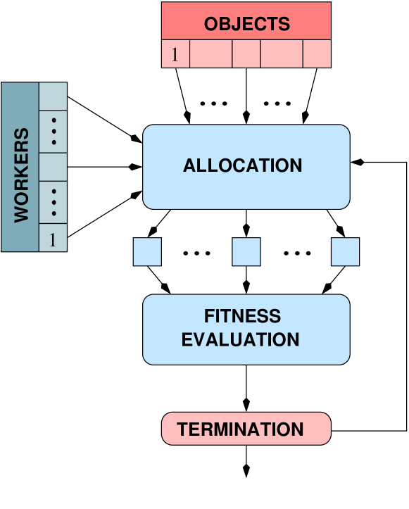
Figure 1: Block scheme of the proposed algorithms

4 Algorithmic Approach

We investigate a class of adaptive algorithms in which objects are sent out for evaluation through several rounds. In each round, each object receives a given number of evaluations by crowd workers (possibly zero, for some objects). Then, on the basis of all collected workers’ answers, the algorithms take decisions about the opportunity of requesting extra evaluations for a subset of the objects in a further round. If no extra evaluations are carried out, the algorithms terminate and a winner is identified.

More formally, denote with $m^{(\ell)}_{i}$ the number of evaluations the $i$-th object has received in round $\ell$ and with $M^{(\ell)}_{i}$ the total number of evaluations received by object $i$ up to (and including) round $\ell$. We define ${\bf a}_{i}^{(\ell)}=\left[a_{ij}^{(\ell)}\right]$, $j=1,\ldots,M_{i}^{(\ell)}$ as the vector of random variables representing the answers about object $i$ collected up to round $\ell$, and ${\bf A}^{(\ell)}=\left[{\bf a}_{1}^{(\ell)},\dots,{\bf a}_{N}^{(\ell)}\right]$.

At the beginning of round $\ell$, with $\ell\geq 1$, the fitness index $\phi_{i}^{(\ell-1)}$ represents a metric associated with the quality of the object $i$, as a result of processing previous evaluations. If $\phi_{i}^{(\ell-1)}>\phi_{j}^{(\ell-1)}$ then the quality of object $i$ is estimated to be larger than the quality of object $j$. Let the vector of all fitness indices be $\boldsymbol{\phi}^{(\ell-1)}=[\phi_{1}^{(\ell-1)},\ldots,\phi_{N}^{(\ell-1)}]$. For $\ell=1$, i.e., when no evaluations are available yet, fitness indices are equal for all objects, since the object qualities are assumed to be instances of i.i.d random variables.

In round $\ell$, some of the objects may have a fitness index equal to $-\infty$. These objects are not assigned any further evaluation and are out of the contest. Define the contestant set ${\cal C}^{(\ell)}$ at round $\ell$ as the set of objects for which the fitness index is currently larger than $-\infty$, i.e.,

$${\cal C}^{(\ell)}=\left\{i\in\{1,\dots,N\}:\phi_{i}^{(\ell-1)}>-\infty\right\}\,.$$

We remark that, according to our algorithms, the contestant set at round $\ell+1$ is always a (possibly improper) subset of the contestant set at round $\ell$, i.e., ${\cal C}^{(\ell+1)}\subseteq{\cal C}^{(\ell)}$.

On the basis of $\boldsymbol{\phi}^{(\ell-1)}$ and, possibly, of the total number of past assignments ${M}^{(\ell-1)}=\sum_{i=1}^{N}M_{i}^{(\ell-1)}$, the algorithm decides, according to a termination rule, whether to stop or to go on with the rounds. If rounds are stopped, the object with the largest fitness index is declared the winner. Otherwise, a budget of new worker evaluations is assigned to objects. Such budget is dimensioned as

$$[m_{1}^{(\ell)},\dots,m_{N}^{(\ell)}]={\cal A}(\boldsymbol{\phi}^{(\ell-1)},M^{(\ell-1)})$$

where ${\cal A}(\cdot)$ is the $\mathbb{R}^{N}\times\mathbb{N}\to\mathbb{N}^{N}$ allocation function. We assume function ${\cal A}(\cdot)$ to be increasing with respect to the object quality, i.e., our algorithm tends to allocate more workers to objects with top estimated quality, as formally stated below.

Property 1

If $\phi^{(\ell-1)}_{i}<\phi^{(\ell-1)}_{j}$, then $m_{i}^{(\ell)}\leq m_{j}^{(\ell)}$, with $m_{i}^{(\ell)}=0$ if $\phi^{(\ell)}_{i}=-\infty$.

After determining the number of suitable evaluations, the objects are sent to available crowd workers, according to a suitable worker selection policy, and answers are collected. Then, such answers, together with the previous ones, are used to update the fitness vector for next round, $\boldsymbol{\phi}^{(\ell)}$ (and, consequently, ${\cal C}^{(\ell+1)}$). Several algorithms can be devised in accordance to the previous scheme, depending on how we select the different metrics and parameters, such as ${\cal A}(\cdot)$, the fitness index, the worker selection policy and the termination rule.

A graphical representation of the proposed algorithms is depicted in Figure 1.

5 Design Parameters

In this section we design the parameters of the algorithms under the assumption that workers’ answers are unquantized.

5.1 A-posteriori quality estimation

At round $\ell$ of the algorithm, on the basis of the collected answers we can compute an a-posteriori distribution $f_{{\bf q}}^{(\ell)}({\bf x}|{\bf Y}^{(\ell)})$ for the quality vector ${\bf q}$, where ${\bf Y}^{(\ell)}$ represents a realization of the random vector ${\bf A}^{(\ell)}$ and collects all the answers up to round $\ell$.

In order to find $f_{{\bf q}}^{(\ell)}({\bf x}|{\bf Y}^{(\ell)})$, let us rewrite in matrix form the relationship between the quality values, the biases and the workers’ answers as

$${\bf Y}^{(\ell)}=\left[\begin{array}[]{cc}\boldsymbol{\Gamma}^{(\ell)}_{{\bf x}}&\boldsymbol{\Gamma}^{(\ell)}_{{\bf b}}\end{array}\right]\left[\begin{array}[]{c}{\bf x}\\ {\bf b}\end{array}\right]+{\bf n}^{(\ell)}$$ (1)

where

• $\boldsymbol{\Gamma}^{(\ell)}_{{\bf x}}$ is a $M^{(\ell)}\times N$ binary allocation matrix, whose $j$-th row has a single 1, located in column $i$ if the $j$-th answer in ${\bf Y}^{(\ell)}$ is an evaluation for object $i$;

• $\boldsymbol{\Gamma}^{(\ell)}_{{\bf b}}$ is a $M^{(\ell)}\times W$ binary allocation matrix, whose $j$-th row has a single 1, located in column $w$ if the $j$-th answer in ${\bf Y}^{(\ell)}$ is an evaluation of worker $w$;

• ${\bf n}^{(\ell)}$ is a vector of uncorrelated Gaussian random variables with zero mean and variance $\sigma^{2}$.

Let $\boldsymbol{\Gamma}^{(\ell)}=\left[\begin{array}[]{cc}\boldsymbol{\Gamma}^{(\ell)}_{{\bf x}}&\boldsymbol{\Gamma}^{(\ell)}_{{\bf b}}\end{array}\right]$ be the overall allocation matrix and $\boldsymbol{\theta}=\left[\begin{array}[]{cc}{\bf x}\mathsf{{}^{T}}&{\bf b}\mathsf{{}^{T}}\end{array}\right]\mathsf{{}^{T}}$ be the set of all parameters to be estimated. Thanks to Bayes’ rule, the joint a-posteriori distribution of ${\bf q}$ and $\boldsymbol{\beta}$ can be written as:

$$f^{(\ell)}_{{\bf q},\boldsymbol{\beta}}(\boldsymbol{\theta}|{\bf Y}^{(\ell)})\propto f({{\bf Y}}^{(\ell)}|\boldsymbol{\theta})\prod_{i=1}^{N}f_{q}(x_{i})\prod_{w=1}^{W}f_{\beta}(b_{w})\,.$$ (2)

Let ${\bf Y}^{(\ell)}=\left[\widetilde{{\bf Y}}^{(1)}\mathsf{{}^{T}},\dots,\widetilde{{\bf Y}}^{(\ell)}\mathsf{{}^{T}}\right]\mathsf{{}^{T}}$ where $\widetilde{{\bf Y}}^{(i)}$ are the answers collected at round $i$ only. Similarly let $\boldsymbol{\Gamma}^{(\ell)}=\left[\widetilde{\boldsymbol{\Gamma}}^{(1)}\mathsf{{}^{T}},\dots,\widetilde{\boldsymbol{\Gamma}}^{(\ell)}\mathsf{{}^{T}}\right]\mathsf{{}^{T}}$ where $\widetilde{\boldsymbol{\Gamma}}^{(i)}$ is the allocation matrix for round $i$ only. Then by using the chain rule we can write

$$f({\bf Y}^{(\ell)}|\boldsymbol{\theta}) = f(\widetilde{{\bf Y}}^{(1)},\dots,\widetilde{{\bf Y}}^{(\ell)}|\boldsymbol{\theta})$$

$$= \prod_{i=1}^{\ell}f(\widetilde{{\bf Y}}^{(i)}|\boldsymbol{\theta},{\bf Y}^{(i-1)})$$

Since $\widetilde{{\bf Y}}^{(i)}$ depends on ${\bf Y}^{(i-1)}$ through $\widetilde{\boldsymbol{\Gamma}}^{(i)}$ we can replace ${\bf Y}^{(i-1)}$ by $\widetilde{\boldsymbol{\Gamma}}^{(i)}$ in the previous equation. It follows that

$$f({\bf Y}^{(\ell)}|\boldsymbol{\theta}) = \prod_{i=1}^{\ell}f(\widetilde{{\bf Y}}^{(i)}|\boldsymbol{\theta},\widetilde{\boldsymbol{\Gamma}}^{(i)})$$

$$\propto \prod_{i=1}^{\ell}\exp\left\{-\frac{\|\widetilde{{\bf Y}}^{(i)}-\widetilde{\boldsymbol{\Gamma}}^{(i)}\boldsymbol{\theta}\|^{2}}{2\sigma^{2}}\right\}$$

$$= \exp\left\{-\frac{\|{\bf Y}^{(\ell)}-\boldsymbol{\Gamma}^{(\ell)}\boldsymbol{\theta}\|^{2}}{2\sigma^{2}}\right\}$$

Therefore

$$f^{(\ell)}_{{\bf q},\boldsymbol{\beta}}(\boldsymbol{\theta}|{\bf Y}^{(\ell)})=\kappa{\rm e}^{-\|{\bf Y}^{(\ell)}\mathord{-}\boldsymbol{\Gamma}^{(\ell)}\boldsymbol{\theta}\|^{2}/(2\sigma^{2})}\prod_{i=1}^{N}f_{q}(x_{i})\prod_{w=1}^{W}f_{\beta}(b_{w})$$

where $\kappa$ is such that $\int f^{(\ell)}_{{\bf q},\boldsymbol{\beta}}(\boldsymbol{\theta}|{\bf Y}^{(\ell)}){\rm\,d}\boldsymbol{\theta}=1$.

When the a-priori pdf’s $f_{q}$ and $f_{\beta}$ are Gaussian with means $\mu_{q}$ and $\mu_{\beta}$, and variances $\sigma_{q}^{2}$ and $\sigma_{b}^{2}$, respectively, as a consequence of the fact that the Gaussian distribution is self-conjugate with respect to the Gaussian likelihood function, we easily obtain that $f^{(\ell)}_{{\bf q},\boldsymbol{\beta}}$ is also Gaussian, with covariance matrix

$$\boldsymbol{\Sigma}_{{\bf q},\boldsymbol{\beta}}^{(\ell)}=\left(\frac{\boldsymbol{\Gamma}^{(\ell)}\mathsf{{}^{T}}\boldsymbol{\Gamma}^{(\ell)}}{\sigma^{2}}+\left(\boldsymbol{\Sigma}_{{\bf q},\boldsymbol{\beta}}^{(0)}\right)^{-1}\right)^{-1}$$ (3)

and mean

$$\boldsymbol{\mu}_{{\bf q},\boldsymbol{\beta}}^{(\ell)}=\boldsymbol{\Sigma}_{{\bf q},\boldsymbol{\beta}}^{(\ell)}\left(\frac{\boldsymbol{\Gamma}^{(\ell)}\mathsf{{}^{T}}{\bf Y}^{(\ell)}}{\sigma^{2}}+\left(\boldsymbol{\Sigma}_{{\bf q},\boldsymbol{\beta}}^{(0)}\right)^{-1}\boldsymbol{\mu}_{{\bf q},\boldsymbol{\beta}}^{(0)}\right)$$ (4)

where

$$\boldsymbol{\Sigma}_{{\bf q},\boldsymbol{\beta}}^{(0)}=\left[\begin{array}[]{cc}\sigma^{2}_{q}{\bf I}_{N}&{\bf 0}\\ {\bf 0}&\sigma^{2}_{\beta}{\bf I}_{W}\end{array}\right]\,,\hskip 17.22217pt\boldsymbol{\mu}_{{\bf q},\boldsymbol{\beta}}^{(0)}=\left[\begin{array}[]{c}\mu_{q}{\bf 1}_{N}\\ \mu_{\beta}{\bf 1}_{W}\end{array}\right]\,,$$

being ${\bf I}_{K}$ the size-$K$ identity matrix and ${\bf 1}_{K}$ the length-$K$ all-one column vector. It is worth noting that $\boldsymbol{\mu}_{{\bf q},\boldsymbol{\beta}}^{(\ell)}$ is the Minimum-Mean-Square-Error estimate of $\boldsymbol{\theta}$ given that ${\bf Y}^{(\ell)}$ is the realization of ${\bf A}^{(\ell)}$. Observe that (3)-(4) also hold for unknown prior distribution, in which case we set $\sigma_{x}=\sigma_{b}=\infty$. Moreover, we remark that (3)-(4) can also be employed to obtain an approximate a-posteriori distribution in the case of non-Gaussian priors with given means and variances.

From the above joint a-posteriori distribution of ${\bf q}$ and $\boldsymbol{\beta}$, it is straightforward to obtain the marginal a-posteriori distribution of ${\bf q}$ in round $\ell$, i.e., $f_{{\bf q}}^{(\ell)}({\bf x}|{\bf Y}^{(\ell)})$. For Gaussian priors, $f_{{\bf q}}^{(\ell)}({\bf x}|{\bf Y}^{(\ell)})$ is Gaussian, with mean $\boldsymbol{\mu}_{{\bf q}}^{(\ell)}=\left[\mu_{q_{1}},\dots,\mu_{q_{N}}\right]$ and covariance matrix $\boldsymbol{\Sigma}_{{\bf q}}^{(\ell)}$ that are equal to the upper part of $\boldsymbol{\mu}_{{\bf q},\boldsymbol{\beta}}^{(\ell)}$ and to the upper-left corner of $\boldsymbol{\Sigma}_{{\bf q},\boldsymbol{\beta}}^{(\ell)}$, respectively.

5.2 Possible performance parameters

In order to properly choose the metrics of the crowdsourcing algorithm, it is important to identify the performance parameters we may want to optimize. Several options can be devised. In the following, we will omit the round index $\ell$ for ease of notation. Consider an answer realization ${\bf Y}=[{\bf y}_{1},\dots,{\bf y}_{N}]$ and define the corresponding estimate $\widehat{i^{*}}({\bf Y})$ of $i^{*}$, in the following simply denoted by $\widehat{i^{*}}$. A set of possible performance parameters that can be considered are:

• the order-$k$ distortion $D^{(k)}=\mathbb{E}\left|q_{\widehat{i^{*}}}-q_{i^{*}}\right|^{k}$, $k\in\mathbb{N}$, which is averaged with respect to the current a-posteriori distribution of ${\bf q}$ given ${\bf A}={\bf Y}$. Unfortunately the computation of the distortion is in general too complex, even for moderate values of $N$.

• the error probability $p_{\rm e}=\mathbb{P}\left\{\widehat{i^{*}}\neq i^{*}\right\}$. With such a choice, a maximum-a-posteriori (MAP) rule turns out to be optimal. Precisely, let $\pi_{i}=\mathbb{P}\{i^{*}=i|{\bf Y}\}$ be the probability of $i$ to be the top-quality object, given the answers ${\bf Y}$, for $i\in{\cal C}$, which is the contestant set. We can in principle compute the value of $\pi_{i}$ as

  $$\pi_{i} = \mathbb{P}\left\{\cap_{j\in{\cal C}\setminus\{i\}}\{q_{j}\mathord{<}q_{i}\}|{\bf Y}\right\}$$ (5)

  $$= \int_{-\infty}^{+\infty}\left(\int_{-\infty}^{x_{i}}\cdots\int_{-\infty}^{x_{i}}f_{{\bf q}}({\bf x}|{\bf Y})\mathbf{{\rm\,d}}^{N-1}{\bf x}_{\sim i}\right){\rm\,d}x_{i}$$

  where ${\bf x}_{\sim i}$ is obtained by removing the $i$-th component from ${\bf x}$. It is easy to see that $p_{\rm e}$ is minimized when $\widehat{i^{*}}=\arg\max_{i}\pi_{i}$.

  Since the evaluation of $\pi_{i}$, for $i=1,\ldots,N$, entails a computational complexity growing linearly with $N$, we propose the following approximation:

  $$\widetilde{\pi}_{i} = \int_{-\infty}^{+\infty}\left(\int_{-\infty}^{x}f_{q_{i},q_{c(i)}}(x,x^{\prime}|{\bf Y}){\rm\,d}x^{\prime}\right){\rm\,d}x$$ (6)

  where $c(i)=\arg\max_{j\neq i}\mu_{q_{j}}$ corresponds to the object with maximum current estimated quality except $i$. In practice, (6) restricts the comparison to only two objects, the running candidate $i$ and its strongest competitor $c(i)$, and uses the current probability $\widetilde{\pi}_{i}({\bf Y})$ that object $i$ is better than $c(i)$ as an approximation for $\pi_{i}({\bf Y})$. Therefore, by construction, $\widetilde{\pi}_{i}\geq{\pi}_{i}$, and the difference decreases as the number of objects with a good estimated quality decreases, as in the last rounds of the algorithm. In the case of Gaussian or unknown priors, (6) becomes

  $$\widetilde{\pi}_{i}=\frac{1}{2}\left[1+{\rm erf}\left(\frac{\mu_{q_{i}}-\mu_{q_{c(i)}}}{\sqrt{2\left(\sigma_{q_{i}}^{2}+\sigma_{q_{c(i)}}^{2}-2\rho_{i,c(i)}\sigma_{q_{i}}\sigma_{q_{c(i)}}\right)}}\right)\right]$$ (7)

  where $\sigma_{q_{i}}^{2}$ and $\rho_{i,j}$ are the current a-posteriori variance for $q_{i}$ and correlation coefficient between $q_{i}$ and $q_{j}$, respectively.

In this work, because of complexity considerations, we choose the error probability as the performance parameter. Therefore our algorithms will be designed in order to reduce the error probability as much as possible.

5.3 Fitness indices

Different choices for fitness indices are possible.

• Exact max probability: we identify the fitness index of objects with their estimated probability of being the top-quality object: $\phi_{i}=\pi_{i}$ whose expression is given in (5).

• Approximate max probability: $\phi_{i}=\widetilde{\pi}_{i}$ whose expression is given in (6).

• Exact max probability with elimination: As stated in the previous section, the contestant set, ${\cal C}$, initially set to $\{1,\dots,N\}$, may be shortened along rounds. We have considered a strategy where, at each round, those objects whose $\pi_{i}$ is lower than a threshold $\pi_{\rm th,E}$ are eliminated. For this strategy, the fitness index is given by:

  $$\phi_{i}=\left\{\begin{array}[]{rl}\pi_{i},&\pi_{i}>\pi_{\rm th,E}\text{ and }i\in{\cal C}\\ -\infty,&\pi_{i}\leq\pi_{\rm th,E}\text{ or }i\notin{\cal C}\end{array}\right.$$ (8)

• Approximate max probability with elimination: we can consider a strategy where objects are eliminated if $\widetilde{\pi}_{i}$ falls below a threshold $\pi_{\rm th,E}$. The corresponding fitness index is given by (8) where $\pi_{i}$ is replaced by $\widetilde{\pi}_{i}$.

All these fitness indices have been tested numerically.

5.4 Allocation function

As stated in previous sections, given the current fitness index, the allocation function ${\cal A}(\cdot)$ determines the number of further evaluations needed by each object in round $\ell$. Furthermore, ${\cal A}(\cdot)$ is a non-decreasing function of the fitness index (Property 1).

For simplicity, we are particularly interested in the case where ${\cal A}(\cdot)$ returns values in $\{0,1\}^{N}$, i.e., where the number of workers assigned to every object within a round is either 0 or 1. In such a case, in round $\ell$, the $B^{(\ell)}\leq N$ top-quality objects will receive an extra worker, while all other objects will not receive any extra worker.

Two possible choices are considered in this paper, according to whether the total evaluation budget is either fixed or not.

• Unbounded budget: If there is no maximum number of requested evaluations, ${\cal A}$ only depends on the fitness index, in the following way: $m_{i}^{(\ell)}=1$ if $\phi_{i}^{(\ell)}>\pi_{\rm th,A}$ and $m_{i}^{(\ell)}=0$ otherwise. Here $\pi_{\rm th,A}$ is a suitable accuracy threshold, generally different from $\pi_{\rm th,E}$ defined in the previous subsection. However, for consistency, we need to have $\pi_{\rm th,E}\leq\pi_{\rm th,A}$. It is worth noting that the value of $\pi_{\rm th,A}$ determines the trade-off between exploitation and exploration: a large value of $\pi_{\rm th,A}$ leads to concentrate the evaluations on objects with a high fitness index (exploitation), while a small $\pi_{\rm th,A}$ will spread equally the evaluations over most objects (exploration). A similar comment applies to the choice of $\pi_{\rm th,E}$.

• Bounded budget: If at most $M_{\rm max}$ evaluations can be requested in all rounds, then, in round $\ell$, ${\cal A}(\cdot)$ must take into account also the number of evaluations already requested, given by $M^{(\ell-1)}$. Let again $\pi_{\rm th,A}$ be the threshold against which the fitness index is compared, like in the unbounded-budget case, and let $B^{(\ell)}$ be the number of objects that currently pass the threshold. If $B^{(\ell)}\leq M_{\rm max}-M^{(\ell-1)}$, then the allocation of new evaluations is the same as for unbounded budget, otherwise only the $M_{\rm max}-M^{(\ell-1)}$ objects with the largest fitness index are allocated a further evaluation.

5.5 Worker selection

Observe that when either worker’s bias is negligible, or it is perfectly known by the system, workers are indistinguishable. Any possible non-degenerate (i.e. according to which every object is evaluated at most once by every worker) allocation of objects to workers will lead to the same performance. When bias comes to play a significant role, things become more involved. Restricting our discussion to the case in which workers’ bias is completely unknown to the system before the allocation, we can make the following considerations:

• to improve the accuracy of the workers’ bias estimate, the worker selection strategy should maximize the number of evaluation performed by every involved worker, while minimizing the number of involved workers. In this way, indeed, on the one hand we minimize the number of parameters to be estimated, while, on the other hand, we maximize the number of available samples for every parameter to be estimated.

• worker bias plays an insignificant role in the case in which, at every round $l$, all the contestant objects in ${\cal C}^{(l)}$ have been evaluated by exactly the same set of workers and answers are unquantized. This because, in this case, for the cumulative effect of the bias of workers, all object evaluations are subject to the same shifts and, therefore, the relative merit among objects (i.e differences among object qualities) are not impacted by worker bias.

  The worker selection strategy we propose is inspired by previous considerations. We assume that every worker can evaluate a limited number of objects. Let us denote with $O_{\rm max}$ the maximum number of allocations for every worker (for the sake of simplicity we assume $O_{\rm max}$ to be the same for every worker, but the extension to the more general case is pretty straightforward). Furthermore, to allow workers to better plan their work, we require that every worker receives all the allocations in a unique batch (i.e., the same worker cannot be employed over multiple rounds). Our allocation policy works as follows: as long as ${\cal C}^{(l)}\leq O_{\rm max}$, at every round we allocate all the contestant objects to a randomly selected new worker. As long as ${\cal C}^{(l)}>O_{\rm max}$, instead, we select $W^{(l)}=\lceil{\cal C}^{(l)}/O_{\rm max}\rceil$ new workers and we allocated to every worker either $\lfloor{\cal C}^{(l)}/W^{(l)}\rfloor$ or $\lceil{\cal C}^{(l)}/W^{(l)}\rceil$ randomly selected objects so to allocate all the contestant objects to the workers.

5.6 Termination rules

Based on the choice of the fitness index and the allocation function ${\cal A}$, the algorithm termination rule may be different.

• Maximum budget achieved: When a maximum of $M_{\rm max}$ evaluations is allowed, reaching this maximum budget will cause rounds to stop.

• Singleton contestant set: For algorithms that eliminate objects when their fitness is lower than $\pi_{\rm th,E}$, the natural termination condition is when the contestant set only contains a single object, i.e., $|{\cal C}^{(\ell)}|=1$.

• Accuracy: If only a single object passes the accuracy threshold $\pi_{\rm th,A}$, while all other objects do not, meaning that there is already a strong candidate winner, the algorithm may terminate rounds.

When applicable, the termination rule can be the combination of all three rules above, i.e., the algorithm may terminate whenever one of the three becomes true.

6 Scoring Versus Direct Comparisons

The goal of this section is to provide a critical comparison between the performance of algorithms based on (noisy) quantitative estimates of the object quality and algorithms just resorting to direct comparisons among subsets of objects. In order to do this, we focus in this section on a toy scenario for which the analysis is tractable. However, we remark that such scenario includes the most significant features of a more complex case.

We start focusing on a simplified scenario in which worker bias can be negligible and we show that, in such a case, the former class of algorithms appears clearly more effective than the latter. Let us first consider a toy case in which only two objects are given, with qualities $x_{1}$ and $x_{2}=x_{1}+\Delta$, and compare two algorithms requiring the same amount of human effort. The first algorithm resorts to outcomes of direct comparisons between the objects performed by the crowd workers, while the second exploits quantitative estimates of the object qualities provided by the same (or other) crowd workers.

Observe that an algorithm exploiting the outcomes of direct comparisons between objects, and employing a fixed budget of $W$ workers for each comparison, necessarily works as follows. Each of the $W$ enrolled workers returns a binary variable, indicating which object she prefers. Once all answers, collectively denoted ${\bf Z}$, are obtained, a majority rule is applied by the algorithm to choose the “best” object. According to our model, each worker prefers object $1$, if she estimates that the quality of object $1$ exceeds the quality of object $2$ and vice versa. Thus, a worker chooses object 1, i.e., returns an incorrect answer, with probability $p_{\Delta}=\frac{1}{2}\text{erfc}(\frac{\Delta}{2\sigma})$, while she chooses object $2$, thus returning a correct answer, with probability $1-p_{\Delta}$.

Processing the $W$ collected answers (to simplify the analysis, we assume an odd value for $W$), the algorithm based on comparisons erroneously selects object $1$ whenever the number of answers equal to 1 exceeds $W/2$, i.e.:

$$p^{\text{comp}}_{\rm e}=\mathbb{P}\left(\text{Bin}(W,p_{\Delta})>W/2\right)$$

where $\text{Bin}(W,p)$ denotes a binomial distribution of parameters $W$ and $p$.

Instead, an algorithm that has access to the quantitative quality estimates ${\bf Y}$ provided by the $W$ crowd workers, naturally selects the object with the largest estimated quality $\widehat{x}({\bf y}_{i})$. In this case the error probability is given by:

$$p^{\text{est}}_{\rm e}=\frac{1}{2}\text{erfc}\left(\frac{\sqrt{W}\Delta}{2\sigma}\right)\,.$$

Figure 2 shows that $p^{\text{est}}_{\rm e}<p^{\text{comp}}_{\rm e}$. Indeed, from an information-theoretic perspective, the answers ${\bf Y}$ provide much more information on the quality of the two objects than the comparisons ${\bf Z}$. This implies that any algorithm resorting to direct comparisons does not fully exploit the information on object quality that crowd workers are able to provide and, as a consequence, turns out to be suboptimal.

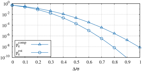
Figure 2: Comparison between quantitative quality estimations and direct comparisons in terms of error probability in the case of two objects. $W=101$.

We now analytically compare $p^{\text{comp}}_{\rm e}$ and $p^{\text{est}}_{\rm e}$ to better quantify the advantages of the approach exploiting quantitative estimates of object quality. To this end, we approximate the binomial distribution $\text{Bin}(W,p_{\Delta})$ with a Gaussian distribution ${\cal N}(Wp_{\Delta},\sqrt{Wp_{\Delta}(1-p_{\Delta}}))$. By the De Moivre-Laplace theorem, such approximation is asymptotically tight for large $W$. Following this approach, $p^{\text{comp}}_{\rm e}$ can be approximated as:

$$p^{\text{comp}}_{\rm e}\approx\frac{1}{2}\text{erfc}\left(\frac{\sqrt{W}(1-2p_{\Delta})}{2\sqrt{2p_{\Delta}(1-p_{\Delta})}}\right)$$

To further simplify the expression of $p^{\text{comp}}_{\rm e}$, we consider the limit for $\frac{\Delta}{\sigma}\to 0$, in which case $p_{\Delta}=\frac{1}{2}\left(1-\frac{2}{\sqrt{\pi}}\frac{\Delta}{2\sigma}\right)+o(\frac{\Delta}{\sigma})$, and thus

$$p^{\text{comp}}_{\rm e}\approx\frac{1}{2}\text{erfc}\left(\sqrt{\frac{2}{\pi}}\frac{\sqrt{W}\Delta}{2\sigma}+o\left(\frac{\Delta}{\sigma}\right)\right)$$

The performance penalty entailed by the approach resorting to direct comparisons of objects is expressed by the factor $\sqrt{2/\pi}$ appearing in the argument of the above erfc function. This factor has a strong impact on the algorithm performance, since, for $\Delta/\sigma$ sufficiently small, as $W$ increases, the ratio $p^{\text{est}}_{\rm e}/p^{\text{comp}}_{\rm e}$ tends exponentially fast to zero.

Now, consider a case in which $N>2$ objects are to be evaluated. For example, let us focus on the case $N=4$. To declare a winner through direct comparisons of objects, we need to compare at least three pairs of objects. A natural solution is to arrange a tournament in which the four objects are first partitioned into two pairs, so that the objects in each pair can be compared in parallel (first round). The two winners of the first round are then compared to identify the globally best object (second round). Observe that the outcomes ${\bf Z}$ returned by crowd workers within the first round cannot be exploited in any way at the second round. In other words, at the end of the first round, no useful information is available to rank the two first-round winners. If, instead, the workers return their own quantitative evaluations ${\bf Y}$ of the object quality, the evaluations carried out within the first round provide useful information also for the second round.

In light of this discussion, it should not be surprising that the performance gain of algorithms exploiting workers’ quantitative quality evaluations increases as the number of objects increases.

Instead, when worker’s bias come to play a significant role, it is a-priori much less clear whether algorithms resorting on absolute (noisy) evaluations are still preferable with respect to algorithms based on direct comparisons. This happens because, while we may expect that the performance of the first tend to degrade for effect of the worker’s bias, the performance of the latter are intrinsically insensitive to the worker’s bias.

However, we wish to highlight that i) as already mentioned, the impact of worker bias on the algorithm performance plays a marginal role, as all the contestant objects are evaluated by the same worker, ii) the worker’s bias can be rather accurately estimated and subtracted when the worker has evaluated a sufficiently large number of objects. The combination of i) and ii) makes us pretty confident that algorithms resorting on absolute quality estimations of objects quality can be still competitive even when worker’s bias is significant. Results presented in the following in Section 8 will confirm our intuition.

7 Answer Quantization

Up to now, we have assumed that workers return unquantized (i.e., infinite-precision) noisy evaluations of object qualities. This assumption is unpractical in many scenarios, where instead workers’ evaluations must belong to a finite alphabet, i.e., they are quantized. In this section, we discuss how quantization can be effectively implemented in order to approach the performance of the proposed unquantized algorithms.

From a system point-of-view, the key parameter of a quantizer is the cardinality $L$ of the alphabet on which answers should be encoded, i.e., the number of levels of the quantizer. Given $L$, a specific quantization rule is characterized by an $(L+1)$-dimensional vector of thresholds ${\cal Z}=[z_{1},\cdots,z_{l},\cdots,z_{L+1}]$ with $z_{1}=-\infty<z_{2}<z_{3}<\cdots,z_{L}<z_{L+1}=+\infty$ and an $L$-dimensional vector ${\cal W}=[w_{1},\cdots,w_{l}\cdots,w_{L}]$ of representative values, satisfying $w_{l}\in(z_{l},z_{l+1})$ If workers’ answers are quantized, then the $j$-th answer to the evaluation of object $i$ can be modeled as

$$a_{ij}^{(\rm q)}={\cal Q}(a_{ij})$$

where ${\cal Q}(x)=w_{l}$ whenever $x\in(z_{l},z_{l+1}]$. Notice that we consider here a fixed, non-adaptive quantizer, that is defined once and for all at the beginning, before any evaluation takes place.

In our context, the problem of optimal quantization can be formulated in terms of the minimization of some distortion index between unquantized answers and their quantized version. The mean square error $\mathbb{E}[(a^{(\rm q)}-a)^{2}]$ represents a natural candidate for such distortion index, also because the seminal work by Lloyd [Lloyd (2006)] provides an efficient iterative algorithm for the design of a quantizer that minimizes the mean square error. Now, the nontrivial question to be answered is: which are the answers whose distortion after quantization should be minimized? We list in the following a few possible answers to such question.

• Since we have $N$ objects whose quality values are i.i.d., each with pdf $f_{q}$, we may want to minimize the distortion on the answer relative to the generic object. With such a choice, the distribution with respect to which the mean square error is to be computed is $f_{a}^{(I)}=f_{q}*f_{n}$, where $*$ is the convolution product and $f_{n}=\mathcal{N}(0,\sigma_{b}^{2}+\sigma^{2})$ is the distribution of the workers’ evaluation error.

• From a different perspective, since we are searching for the top-quality object, we should minimize the distortion on the answers associated to that object only, i.e., averaging with respect to $f_{a}^{(II)}=f_{q_{[1]}}*f_{n}$, $f_{q_{[1]}}$ being the a-priori distribution of the largest quality value.

• Taking an approach which is in-between the previous two, and considering that our target is to discriminate the best object from the others, we could aim at minimizing a weighted combination of the distortions relative to the ordered quality values. This goal can be achieved by using as the answer distribution $f^{(III)}_{a}=\sum_{i=0}^{N-1}\alpha_{i}f_{q_{[i]}}*f_{n}$, where $f_{q_{[i]}}$ is the a-priori distribution for the $i$-th best object, and $\alpha_{i}$ is its associated weight, satisfying $\alpha_{i+1}\leq\alpha_{i}$.

We point out that, in order to better adapt to the distribution of objects to be evaluated, the quantizer should be redesigned at each round instead of just once at the beginning. This, however, entails a significant complexity increase of the algorithm. For the sake of simplicity in the following we will design the quantizer only once.

In the next section we show that the impact on algorithm performance of the different possible choices for $f_{a}$ is pretty significant. Therefore, the quantizer must be carefully designed. Finally, observe that $f^{(I)}_{a}$ and $f^{(II)}_{a}$ can be obtained as particular cases of $f^{(III)}_{a}$ by setting $\alpha_{i}=1/N$ for all $i$ in the first case, and $\alpha_{1}=1$, $\alpha_{i}=0$ for $i>1$ in the second case.

8 Results

In this section, we compare the performance of several algorithms that are obtained by making different choices for the fitness index, the allocation function, the termination rule, and the quantizer. In Section 8.1 we first focus on a simple scenario where object qualities are equally spaced, the budget is unbounded (i.e., we can employ an unlimited number of evaluations), workers do not suffer from bias and provide unquantized answers. Then, in Sections 8.2 and 8.3 we will show the effects of bounded budget and bias on system performance. We conclude by analyzing the effect of quantized answers in Section 8.4.

8.1 Algorithm comparison in a simple scenario

In particular, we first focus on algorithms with unquantized answers and unbounded budget, and define:

• the ’Greedy-Keep-Exact’ (GKE) algorithm, employing the exact max probability as fitness index, unbounded budget as allocation function, and the accuracy termination rule;

• the ’Greedy-Keep-Approximate’ (GKA) algorithm, employing the approximate max probability as fitness index, the unbounded budget as allocation function, and the accuracy termination rule;

• the ’Greedy-Remove-Approximate’ (GRA) algorithm, employing the approximate max probability with eliminations as fitness index, the unbounded budget as allocation function, and singleton contestant set as termination rule.

To reduce the space of parameters, we have always fixed $\pi_{\rm th,A}=\pi_{\rm th,E}\triangleq\pi_{\rm th}$. For the sake of comparison, the following algorithms have been also considered.

• We have superimposed a classical tournament scheme to our previously described algorithms, obtaining a family of Tournament-$N_{b}$ (T-$N_{b}$) algorithms. Specifically, in T-$N_{b}$ algorithms, the $N$ objects to be evaluated are first randomly partitioned into subgroups of size $N_{b}$ (for simplicity, we neglect rounding problems). The GKA algorithm is then run to elect a winner for each of the object groups. Only winners have access to the second stage, in which again objects are partitioned into subgroups of size $N_{b}$ and winners are elected for each subgroup. The process is iterated until only one winner is left. We remark that our tournament schemes effectively exploit, at every stage, full information about the evaluations of competing objects collected at earlier stages.

• A non-adaptive algorithm, which assigns to every object a fixed number of workers, referred to as Uniform algorithm (UA).

• As a reference, we have also considered an unfeasible Genie-Aided (GA) algorithm, which has access to the identity of the two best competing objects, after a first initial round of evaluations, where every object receives one score. Therefore, in the following rounds, the GA algorithm equally distributes workers only to the top two objects until the accuracy termination rule is met. Observe that, by construction, the performance of the GA algorithm constitutes an upper bound for every feasible algorithm, since, as discussed in Section 6, it implements the optimal policy to find the best between two objects.

We start considering a simple scenario with $N=16$ objects whose qualities $x_{i}$ are equally spaced in the interval $[-1,1]$, so that the smallest difference between quality values is $\Delta=\frac{2}{N-1}=\frac{2}{15}$. The standard deviation of the worker evaluation error has been set to $\sigma=\Delta/2$.

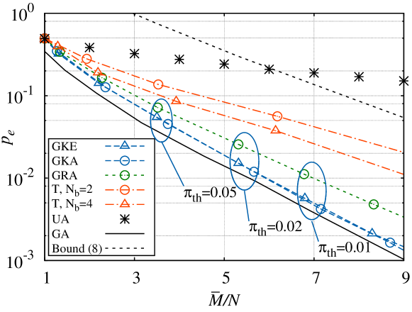
Figure 3: Performance ($p_{\rm e}$ vs $\overline{M}/N$) of different algorithms with unquantized answers, no bias, and unbounded budget for equally spaced objects, $N=16$, $\Delta/\sigma=2$.

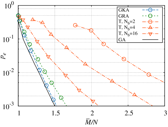
Figure 4: Performance ($p_{\rm e}$ vs $\overline{M}/N$) of different algorithms with unquantized answers, no bias, and unbounded budget for equally spaced objects, $N=256$, $\Delta/\sigma=2$

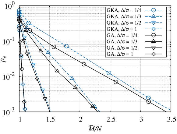
Figure 5: Performance ($p_{\rm e}$ vs $\overline{M}/N$) of different algorithms with unquantized answers, no bias, and unbounded budget for equally spaced objects, $N=256$, and varying $\Delta/\sigma$.

Fig. 3 shows the results obtained with the different proposed algorithms, plotted in terms of error probability $p_{\rm e}$ versus the average number of performed evaluations per object $\overline{M}/N$. We highlight that the different trade-offs between $p_{\rm e}$ and $\overline{M}/N$ correspond to different values of the threshold $\pi_{\rm th}$. Precisely, in Fig. 3, blue circles group results obtained with the same values of $\pi_{\rm th}$. Observe that the choice of $\pi_{\rm th}$ has a direct impact on the expected error probability of the algorithm. In particular, for the GKE algorithm a simple analysis yields the following relationship between $\pi_{\rm th}$ and $p_{\rm e}$:

$$p_{\rm e}=\sum_{i\neq\widehat{i}^{*}}\pi_{i}({\bf y})\leq(N-1)\pi_{\rm th}$$ (9)

More in general, for every algorithm, by decreasing $\pi_{\rm th}$ we achieve a larger accuracy at the cost of employing more resources.

From the results, the following observations can be made.

• Every adaptive algorithm performs much better than the uniform algorithm, employing on average the same amount of resources.

• Greedy algorithms without elimination perform better than greedy algorithms with elimination. Observe, however that the latter are preferable in terms of computational complexity, since in such schemes, at round $\ell$, the fitness index has to be computed only for objects in the contestant set ${\cal C}^{(\ell)}$, while in schemes without elimination it has to be computed for all objects.

• The selection of the approximate max probability as fitness index, in place of the exact max probability, does not lead to any appreciable performance degradation, while having a significant beneficial impact on the computational complexity of the algorithm (this has been checked also for algorithms with elimination).

• Tournament algorithms perform worse than our adaptive algorithms; furthermore, their performance tends to worsen as $N_{b}$ is reduced.

• The performance of greedy algorithms without elimination is only marginally worse than that of the GA algorithm.

To gather more insight on the algorithm behavior, a further performance comparison for the different schemes is reported in Fig. 4 for the case in which the number of objects is increased to $N=256$ (object qualities $x_{i}$ are still equally spaced in the interval $[-1,1]$, with $\sigma=\Delta/2$). Observe that the relative ranking among the algorithms does not change, but the performance gap between algorithms tends to become more significant. In particular, tournament algorithms perform much worse than GKA and GRA. We remark that our results seem somehow in contrast with findings in [Khan and Garcia-Molina (2014)], where it has been shown that tournament algorithms provide the best performance, for cases in which users are only able to compare objects pairs. To intuitively grasp why they become inefficient in our context as $N$ increases, notice that tournament algorithms waste a significant amount of resources to discriminate among objects with similar quality (accidentally placed in the same group), even when the quality of such objects is much worse than top-quality values. Observe that, also in this case, GKA (whose performance is again practically indistinguishable from GKE, not reported in Fig. 4 for the sake of readability) performs similarly to the GA algorithm. This proves the effectiveness of GKA in the considered scenarios.

To evaluate the impact of human evaluation errors on the overall performance of algorithms, Fig. 5 reports a performance comparison between the GKA and GA algorithms for different values of the parameter $\Delta/\sigma$. Observe that $\Delta/\sigma$ plays an important role: as the ratio $\Delta/\sigma$ decreases, more and more resources are needed to meet the same error probability. The performance gap between the two algorithms is rather limited in all cases. In particular, uniformly over all cases, the penalty cost in terms of evaluations required to obtain the same error probability does not exceed 10%. Once again, this confirms the effectiveness of our approach for a broad range of scenarios where evaluation errors have different impact.

8.2 Effects of bounded budget

Now, we move to scenarios in which the budget of allocations is bounded, and we restrict our analysis to:

• the ’bounded-Greedy-Keep-Approximate’ (bGKA), employing the approximate max probability as fitness index, the bounded budget as allocation function, the maximum budget achieved or accuracy termination rule;

• the ’bounded-Greedy-Remove-Approximate’, (bGRA) employing the approximate max probability with eliminations as fitness index, the bounded budget as allocation function, the maximum budget achieved or singleton contestant list as termination rule.

As a reference, we report also the performance of the bounded version of the GA algorithm (bGA), which again provides an obvious upper bound to performance. Also in this case, to reduce the space of parameters, we fix $\pi_{\rm th}=\pi_{\rm th,A}=\pi_{\rm th,E}$.

Fig. 6 compares the performance of different algorithms for different values of the normalized budget $K=M_{\rm max}/N$. In the same figure, we also report the performance of the unbounded versions of the algorithms. We observe that:

• the error probability for bGKA and bGRA now is not monotonic with respect to $\overline{M}/N$. In particular, if the average number of evaluations $\overline{M}$ is sufficiently smaller than $M_{\rm max}$ (i.e., for sufficiently large values of $\pi_{\rm th}$), the performance of the bounded algorithms does not significantly differ from the respective unbounded version: this happens because the probability that the algorithm terminates for achieving maximum budget is negligible. As we further reduce $\pi_{\rm th}$, increasing the required accuracy, the probability that the algorithm terminates because the maximum budget is achieved quickly increases, and the overall performance of the bounded algorithms degrades. These effects can be better understood from Fig 7, which reports the average number of evaluations per object, $\overline{M}/N$, and the error probability, as a function of the threshold $\pi_{\rm th}$, for the bGKA algorithm (similar considerations hold for bGRA). Now, observe that $\overline{M}/N$ monotonically increases as $\pi_{\rm th}$ decreases, since, by decreasing $\pi_{\rm th}$, the algorithm tends to be more conservative in excluding objects from receiving further evaluations. As a result, we distribute a larger number of allocations to objects with a quality quite distant from the maximum. While the error probability behaves monotonically with respect to $\pi_{\rm th}$ (decreasing as $\pi_{\rm th}$ is decreased) in the case of an unbounded budget, in the case of bounded budget, choosing a value of $\pi_{\rm th}$ too small will lead to an inefficient distribution of the limited resources.

• As a consequence of i), only a limited range of $p_{\rm e}$ values can be achieved in the bounded budget case.

• Also in this case, bGKA outperforms bGRA.

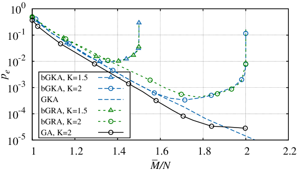
Figure 6: $p_{\rm e}$ vs $\overline{M}/N$ for bGKA and bGRA, $N=256$ equally spaced objects.

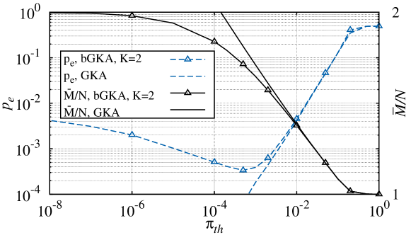
Figure 7: $p_{\rm e}$ and $\overline{M}/N$ vs $\pi_{\rm th}$ for bGKA, $N=256$ equally spaced objects.

Now, we consider a scenario in which object qualities $x_{i}$ are randomly drawn from a Gaussian distribution with zero mean and standard deviation $\sigma_{\rm a}$.

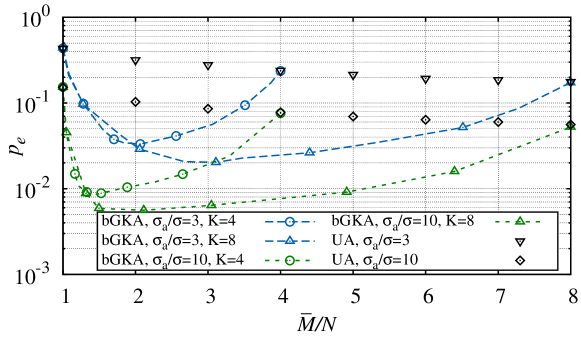
Figure 8: $p_{\rm e}$ vs $\overline{M}/N$ for bGKA and Uniform, $N=256$. Object qualities are Gaussian.

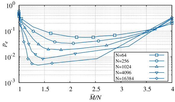
Figure 9: $p_{\rm e}$ vs $\overline{M}/N$ as $N$ varies, for bGKA, $\sigma_{\rm a}/\sigma=3$ and $K=4$. Object qualities are Gaussian.

Fig.  8 presents the performance of bGKA for the cases in which $\sigma_{\rm a}/\sigma=3$ and $\sigma_{\rm a}/\sigma=10$. For the sake of comparison, the figure also reports the performance of the uniform algorithm.

Fig. 9 shows the performance of bGKA algorithm for $\sigma_{\rm a}/\sigma=3$ and $K=4$ as the number of objects, $N$, varies. In particular:

• when the threshold $\pi_{{\rm th},A}=0$ (i.e., when $\bar{M}/N=4$) the algorithm always assigns $K=4$ evaluations to each object. Since as $N$ increases, objects are denser, finding the maximum is more challenging and more prone to errors.

• Instead, when the threshold significantly increases (left part of the figure), the algorithm is able to efficiently allocate the available evaluations on a small set of objects. Since the total budget increases with $N$, the number of evaluations assigned to the best objects increases with $N$ as well. Therefore, as $N$ grows the probability of exhausting the budget decreases. This has a beneficial effect on the overall error probability.

In conclusion we observe that:

• when qualities are drawn from a Gaussian distribution, bGKA improves performance with respect to the uniform allocation algorithm that employs the same average budget of resources;

• from a qualitative point of view, bGKA exhibits a behavior which is pretty similar to the case where objects are equally spaced. By decreasing $\pi_{\rm th}$ we initially increase accuracy at the cost of increasing also the amount of employed resources. However, beyond a given point, further decrements of $\pi_{\rm th}$ cause a loss of efficiency, worsening the overall performance of the algorithm;

• the performance of the algorithms heavily depends on the parameter $\sigma_{\rm a}/\sigma$, which can be regarded as a difficulty index for the problem.

8.3 Effects of bias

In Fig. 10 we show the performance of the bGKA algorithm in the case where workers suffer from bias. We test the algorithm for $N=256$ objects with Gaussian-distributed qualities, $\sigma_{\rm a}=3$, $\sigma=1$, and for different values of the bias variance $\sigma^{2}_{\rm b}$. Moreover, the budget is bounded to $K=8$ and each worker can evaluate up to 256 objects. Observe that even if all the evaluations of a round can be performed by a single worker in bGKA, by construction different objects are evaluated by different sets of workers (indeed, only a subset of contestant objects is evaluated at every round). Therefore worker bias can potentially significantly affect the bGKA performance if not properly compensated.

The solid line refers to the case $\sigma_{\rm b}=0$. Instead, the dashed lines have been obtained for $\sigma_{\rm b}/\sigma=1,2,3$, respectively. As expected, the bias leads to a moderate performance degradation since it is effectively estimated and compensated. We can also observe that the algorithm is weakly sensitive to the bias variance. Indeed, the dashed lines are quite close to each other.

Instead the dash-dotted lines refer to the case where the algorithm does not estimate and compensate for the bias. We see that in this scenario the performance is significantly worsened.

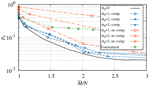
Figure 10: Performance of the bGKA algorithm versus $\overline{M}/N$, with biased workers, $N=256$ objects, Gaussian-distributed qualities, $\sigma_{\rm a}=3$, $\sigma=1$, and for different values of the bias variance $\sigma^{2}_{\rm b}$.

For the sake of comparison we also added the performance of the T-2 algorithm for $\sigma_{\rm b}=0$ which shows considerable performance degradation with respect to the bGKA algorithm with biased workers. Once again we remark that the T-2 algorithm is optimistic with respect to classical comparison algorithms as explained in Section 6.

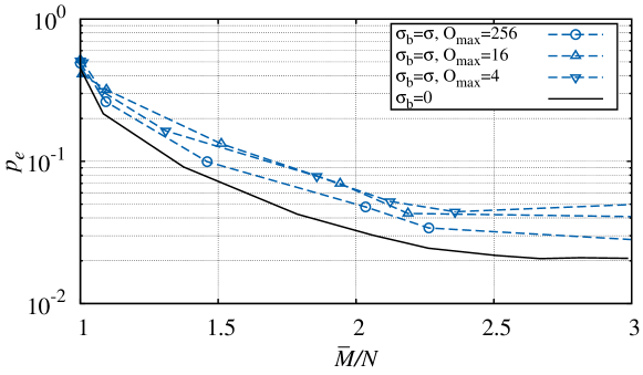
Figure 11: Performance of the bGKA algorithm versus $\overline{M}/N$, with biased workers, $N=256$ objects, $\sigma_{\rm a}/\sigma=3$, $\sigma_{\rm b}/\sigma=1$, $K=8$, and for various values of $O_{\rm max}$.

In Fig. 11 we evaluate the impact of the maximum number of objects that each worker can handle, $O_{\rm max}$ for $N=256$ objects with Gaussian-distributed qualities, $\sigma_{\rm a}/\sigma=3$, $\sigma_{\rm b}/\sigma=1$ and the budget is bounded to $K=8$. As $O_{\rm max}$ decreases a larger number of workers are required to perform the same task and, by consequence, the number of bias parameters to be estimated also increases. However we observe that the degradation is very limited even when $O_{\rm max}=4$.

8.4 Effects of quantization

In Fig. 12, we test the impact of different quantizers, in terms of $p_{e}$ versus $\overline{M}/N$, in the case where $N=256$ objects are equally spaced in the interval $[-1,1]$ and unbiased workers are used. In the figure, the GKA algorithm with unbounded budget is employed for all curves. Moreover, the standard deviation of the worker evaluation error has been set to $\sigma=\Delta/2$. We recall that, for equally spaced objects, $\Delta=2/(N-1)$ is the smallest distance between quality values. The solid line without markers represents the performance of the GKA algorithm without quantization and is used as a benchmark. The line with triangle markers refers to the performance obtained employing a quantizer with $L=32$ representative values uniformly distributed in $[-1-2\sigma,1+2\sigma]$. We observe that, despite of the high number of levels, uniform quantization significantly worsen the error probability. Instead, much better performance is achievable when the quantizer design is more accurate. As an example, the solid line with filled square markers refers to the case when $L=32$, and the quantizer is designed according to the criteria in [Lloyd (2006)], over the answer distribution $f^{(III)}_{a}=\sum_{i=0}^{N-1}\alpha_{i}f_{q_{[i]}}*f_{n}$, where $\alpha_{i}=\gamma^{i}$, and $\gamma=1/2$. This quantizer, labeled “Lloyd” in the legend, provides performance close to the unquantized case. In general, we observe that the performance is quite insensitive to the design parameter $\gamma$ except if its value is close to the extreme point $\gamma=1$. Fig. 12 also shows the performance of Lloyd’s quantizers with $\gamma=1/2$ and number of levels $L=4,8$. We observe that an accurately designed quantizer with only $L=8$ levels is enough to provide performance close to the unquantized case.

Fig. 13 refers to the case of $N=256$ objects with Gaussian-distributed qualities, the budget is bounded to $K=3$, and workers’ answers are quantized. The quantizer is designed according to the Lloyd’s algorithm over the weighted distribution $f^{(III)}_{a}=\sum_{i=0}^{N-1}\alpha_{i}f_{q_{[i]}}*f_{n}$, with $\alpha_{i}=\gamma^{i}$, and $\gamma=1/2$. In the figure, the solid line refers to the unquantized case, while the lines with markers refer to the case where quantization is employed with $L=4,8,16,32$ levels. Also in this scenario, we observe that $L=8$ quantization levels are enough to provide performance close to the unquantized case.

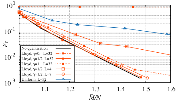
Figure 12: Performance ($p_{\rm e}$ vs $\overline{M}/N$) of the GKA algorithm with unbounded budget and quantized workers’ answers, for $N=256$ objects with equally spaced quality values. Workers’ evaluations are affected by no bias.

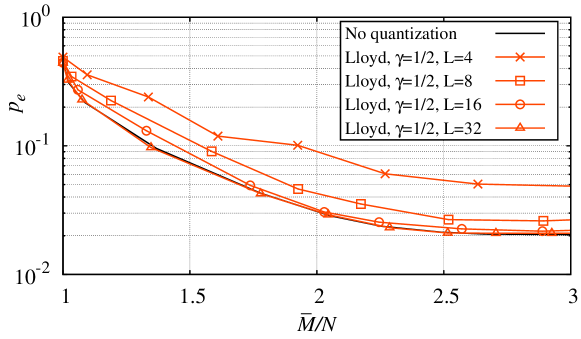
Figure 13: Performance of the GKA algorithm with bounded budget, quantized workers’ answers, for $N=256$ objects with Gaussian-distributed qualities. Workers’ evaluations are affected by no bias.

In Figs. 14 and 15 we combine the effects of bias, quantization and bounded budget with $N=256$ objects with Gaussian-distributed qualities, $\sigma_{\rm a}/\sigma=3$, $\sigma_{\rm b}/\sigma=1$ and $K=8$. The figures show the error probability $p_{e}$ versus the $\bar{M}/N$ for $L=4,8,16$ quantization levels. The cases with unquantized answers and unbiased workers are also reported.

Specifically in Fig. 14 we set $O_{\rm max}=256$ so that at each round a single additional worker (and hence a single bias parameter to be estimated) is required, while in Fig. 15 we considered the more challenging scenario where $O_{\rm max}=16$. In the latter case, at each round, up to 16 workers are required.

We observe that in both cases 16 quantization levels are enough to limit the performance degradation. Surprisingly, for $L=4$ performance worsens with increasing $O_{\rm max}$. This is due to complex interaction between the bias estimation algorithm and the quantizer.

Finally in Figure 16 we investigate the effect of workers with different skills on the system performance. Precisely each worker is characterized by a random evaluation variance, uniformly distributed in $[(1-\epsilon)\sigma^{2},(1+\epsilon)\sigma^{2}]$ where $0\leq\epsilon\leq 1$. The system parameters are the same as in Figure 15 and we consider $L=16$ quantization levels. It can be observed that the impact of random variances is very limited. As a matter of fact, an algorithm able to estimate and exploit such variances would provide better performance at a price of a complexity increase. Such an algorithm could be based on belief propagation as in [Ok et al. (2017)]. However, the results depicted in the figure show that our algorithm is robust and able to handle workers with different skills.

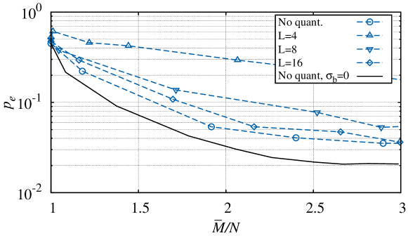
Figure 14: Performance of the GKA algorithm with bounded budget, quantized workers’ answers, for $N=256$ objects with Gaussian-distributed qualities and $O_{\rm max}=256$. Workers’ evaluations are affected by bias.

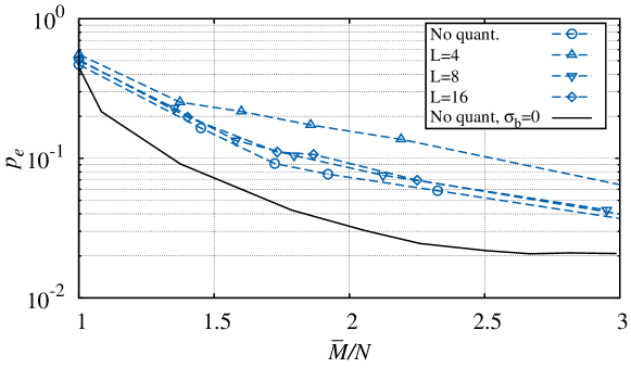
Figure 15: Performance of the GKA algorithm with bounded budget, quantized workers’ answers, for $N=256$ objects with Gaussian-distributed qualities and $O_{\rm max}=16$. Workers’ evaluations are affected by bias.

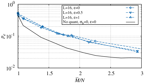
Figure 16: Performance of the GKA algorithm with bounded budget, for $N=256$ objects with Gaussian-distributed qualities $L=16$ and $O_{\rm max}=16$. Workers’ evaluations are affected by bias and their evaluation variance is uniformly distributed with support $[(1-\epsilon)\sigma^{2},(1+\epsilon)\sigma^{2}]$.

9 Design Considerations

In this section we address two important issues: we evaluate the computational complexity of our algorithms, and we discuss how to set algorithm parameters (and in particular $\pi_{\rm th}$). For the sake of brevity, we restrict our investigation to bGKA, which turns out to be the best-performing algorithm.

For what concerns computational complexity, at round $\ell$ and in presence of bias in workers’ answers the bGKA algorithm must

1. compute $\boldsymbol{\mu}_{{\bf q},\boldsymbol{\beta}}^{(\ell)}$ (this operation has complexity $O(N^{3})$ since it requires the computation of the inverse of a $N\times N$ matrix);

2. compute a fitness index $\phi^{(\ell)}_{i}$ for every object (this requires $O(N)$ operations since the approximate max probability can be computed by exploiting (6));

3. compare $\phi^{(\ell)}_{i}$ with $\pi_{\rm th}$, for $i=1,\ldots,N$, in order to decide whether to allocate extra workers (again this requires $O(N)$ operations).

In the final round, if the number of objects that pass the threshold exceeds the residual budget, the execution of an extra task is necessary: objects must be sorted in order of their fitness index (the cost of sorting is notoriously $O(N\log N))$. Observing that $M_{\rm max}$ is an obvious upper bound to the number of rounds, it turns out that the overall complexity of bGKA can be upper-bounded by $O(M_{\rm max}N^{3})$.

Instead, when bias is not estimated, matrix inversion is not required. In such scenario, the complexity of step i) becomes $O(N)$, thus the overall complexity is $O(M_{\rm max}N+N\log N)=O(M_{\rm max}N)$ in consideration of the fact that by construction $M_{\rm max}\geq N$.

As regards the setting of the algorithm parameters, which in the case of bGKA are $\pi_{\rm th}$, $O_{\rm max}$ and $M_{\rm max}$, we observe that the choice of the value for $M_{\rm max}$ normally depends on economical or application-oriented considerations, whose discussion is beyond the scope of this paper. Given the value of $M_{\rm max}$, it is possible to tune the algorithm by selecting the value for $\pi_{\rm th}$, which should be set in order to minimize the error probability. For a careful setting of $\pi_{\rm th}$, a preliminary parametric analysis of the algorithm performance is necessary to estimate the key system parameters (such as the pdf $f_{q}$ of object qualities, the bias variance, $\sigma^{2}_{b}$, and the variance $\sigma$ of the workers’ quality estimation errors).

10 Possible extensions to the top-$k$ object selection

Although we have described our algorithms in a particular setting, our approach can be easily extended to more general scenarios. In particular, it is possible to generalize the approach proposed in this paper to the problem of finding the $k$ top-quality elements within a large collection of objects through crowdsourcing algorithms. Indeed, as an extension of $\pi_{i}$, we can define $\pi_{i}^{(k)}$ as the probability for the $i$-th object to be among the $k$ best. Then, a possible algorithm could divide objects into three categories: i) those that are with high probability within the $k$ best, ii) those that with high probability are not within the $k$ best, and iii) the remaining ones. This can be done by defining two thresholds instead of only one. The mechanism of allocation of new evaluations to objects is a straightforward extensions of the one described in the paper. More precisely, new evaluations are requested at each round only for objects of the third category.

11 Concluding Remarks

In this paper, we have studied the problem of finding the top-quality element within a large collection of objects, resorting to human evaluations affected by noise and by bias. Differently from previous works, our study started assuming that unquantized scores are returned by the evaluators, and highlights the potential advantages of such approach. We have shown that bias can be estimated and compensated with an affordable additional complexity.

Then we have shown how to properly design quantized schemes whose performance is very close to their ideal unquantized counterparts, provided that a reasonable number of quantization levels is assigned to workers’ answers.

References

- [1]
- Agrawal (1995) Rajeev Agrawal. 1995. Sample Mean Based Index Policies with O(log n) Regret for the Multi-Armed Bandit Problem. Advances in Applied Probability 27, 4 (1995), 1054–1078. http://www.jstor.org/stable/1427934
- Auer et al. (2002) Peter Auer, Nicolò Cesa-Bianchi, and Paul Fischer. 2002. Finite-time Analysis of the Multiarmed Bandit Problem. Machine Learning 47, 2 (2002), 235–256. DOI:http://dx.doi.org/10.1023/A:1013689704352
- Azoulay-Schwartz et al. (2004) Rina Azoulay-Schwartz, Sarit Kraus, and Jonathan Wilkenfeld. 2004. Exploitation vs. exploration: choosing a supplier in an environment of incomplete information. Decision Support Systems 38, 1 (2004), 1 – 18. DOI:http://dx.doi.org/https://doi.org/10.1016/S0167-9236(03)00061-7
- Davidson et al. (2013) Susan B. Davidson, Sanjeev Khanna, Tova Milo, and Sudeepa Roy. 2013. Using the Crowd for Top-k and Group-by Queries. In Proceedings of the 16th International Conference on Database Theory (ICDT ’13). ACM, New York, NY, USA, 225–236. DOI:http://dx.doi.org/10.1145/2448496.2448524
- Feige et al. (1994) Uriel Feige, Prabhakar Raghavan, David Peleg, and Eli Upfal. 1994. Computing with Noisy Information. SIAM J. Comput. 23, 5 (1994), 1001–1018. DOI:http://dx.doi.org/10.1137/S0097539791195877
- Guo et al. (2012) Stephen Guo, Aditya Parameswaran, and Hector Garcia-Molina. 2012. So Who Won?: Dynamic Max Discovery with the Crowd. In Proceedings of the 2012 ACM SIGMOD International Conference on Management of Data (SIGMOD ’12). ACM, New York, NY, USA, 385–396. DOI:http://dx.doi.org/10.1145/2213836.2213880
- Ho et al. (2013) Chien-Ju Ho, Shahin Jabbari, and Jennifer Wortman Vaughan. 2013. Adaptive Task Assignment for Crowdsourced Classification. In Proceedings of the 30th International Conference on International Conference on Machine Learning - Volume 28 (ICML’13). JMLR.org, I–534–I–542. http://dl.acm.org/citation.cfm?id=3042817.3042879
- Karger et al. (2011) David R. Karger, Sewoong Oh, and Devavrat Shah. 2011. Iterative Learning for Reliable Crowdsourcing Systems. In Advances in Neural Information Processing Systems 24, J. Shawe-Taylor, R. S. Zemel, P. L. Bartlett, F. Pereira, and K. Q. Weinberger (Eds.). Curran Associates, Inc., 1953–1961. http://papers.nips.cc/paper/4396-iterative-learning-for-reliable-crowdsourcing-systems.pdf
- Karger et al. (2013) David R. Karger, Sewoong Oh, and Devavrat Shah. 2013. Efficient Crowdsourcing for Multi-class Labeling. In Proceedings of the ACM SIGMETRICS/International Conference on Measurement and Modeling of Computer Systems (SIGMETRICS ’13). ACM, New York, NY, USA, 81–92. DOI:http://dx.doi.org/10.1145/2465529.2465761
- Khan and Garcia-Molina (2014) AR Khan and H Garcia-Molina. 2014. Hybrid strategies for finding the max with the crowd. Technical Report. Technical report.
- Khetan and Oh (2016) Ashish Khetan and Sewoong Oh. 2016. Achieving budget-optimality with adaptive schemes in crowdsourcing. In Advances in Neural Information Processing Systems 29, D. D. Lee, M. Sugiyama, U. V. Luxburg, I. Guyon, and R. Garnett (Eds.). Curran Associates, Inc., 4844–4852. http://papers.nips.cc/paper/6124-achieving-budget-optimality-with-adaptive-schemes-in-crowdsourcing.pdf
- Lai and Robbins (1985) T.L Lai and Herbert Robbins. 1985. Asymptotically efficient adaptive allocation rules. Advances in Applied Mathematics 6, 1 (1985), 4 – 22. DOI:http://dx.doi.org/10.1016/0196-8858(85)90002-8
- Liu and Liu (2015) Yang Liu and Mingyan Liu. 2015. An Online Learning Approach to Improving the Quality of Crowd-Sourcing. In Proceedings of the 2015 ACM SIGMETRICS International Conference on Measurement and Modeling of Computer Systems (SIGMETRICS ’15). ACM, New York, NY, USA, 217–230. DOI:http://dx.doi.org/10.1145/2745844.2745874
- Lloyd (2006) S. Lloyd. 2006. Least Squares Quantization in PCM. IEEE Trans. Inf. Theor. 28, 2 (Sept. 2006), 129–137. DOI:http://dx.doi.org/10.1109/TIT.1982.1056489
- Negahban et al. (2012) Sahand Negahban, Sewoong Oh, and Devavrat Shah. 2012. Iterative ranking from pair-wise comparisons. In Advances in Neural Information Processing Systems 25, F. Pereira, C. J. C. Burges, L. Bottou, and K. Q. Weinberger (Eds.). Curran Associates, Inc., 2474–2482. http://papers.nips.cc/paper/4701-iterative-ranking-from-pair-wise-comparisons.pdf
- Ok et al. (2017) Jungseul Ok, Sewoong Oh, Jinwoo Shin, Yunhun Jang, and Yung Yi. 2017. Efficient Learning for Crowdsourced Regression. CoRR abs/1702.08840 (2017). http://arxiv.org/abs/1702.08840
- Thurstone (1927) Louis L Thurstone. 1927. A law of comparative judgment. Psychological review 34, 4 (1927), 273.
- Venetis and Garcia-Molina (2012) Petros Venetis and Hector Garcia-Molina. 2012. Dynamic Max Algorithms in Crowdsourcing Environments. Technical report. Stanford University. http://ilpubs.stanford.edu:8090/1050/
- Venetis et al. (2012) Petros Venetis, Hector Garcia-Molina, Kerui Huang, and Neoklis Polyzotis. 2012. Max Algorithms in Crowdsourcing Environments. In Proceedings of the 21st International Conference on World Wide Web (WWW ’12). ACM, New York, NY, USA, 989–998. DOI:http://dx.doi.org/10.1145/2187836.2187969
- Verroios et al. (2015) Vasilis Verroios, Peter Lofgren, and Hector Garcia-Molina. 2015. tDP: An Optimal-Latency Budget Allocation Strategy for Crowdsourced MAXIMUM Operations. In Proceedings of the 2015 ACM SIGMOD International Conference on Management of Data (SIGMOD ’15). ACM, New York, NY, USA, 1047–1062. DOI:http://dx.doi.org/10.1145/2723372.2749440
- Yuen et al. (2011) M. C. Yuen, I. King, and K. S. Leung. 2011. A Survey of Crowdsourcing Systems. In 2011 IEEE Third International Conference on Privacy, Security, Risk and Trust and 2011 IEEE Third International Conference on Social Computing. 766–773. DOI:http://dx.doi.org/10.1109/PASSAT/SocialCom.2011.203
- Zoghi et al. (2014) Masrour Zoghi, Shimon Whiteson, Remi Munos, and Maarten De Rijke. 2014. Relative Upper Confidence Bound for the K-armed Dueling Bandit Problem. In Proceedings of the 31st International Conference on International Conference on Machine Learning - Volume 32 (ICML’14). JMLR.org, II–10–II–18. http://dl.acm.org/citation.cfm?id=3044805.3044894