Thermodynamics, contact and density profiles of the repulsive Gaudin-Yang model

Abstract

We address the problem of computing the thermodynamic properties of the repulsive one-dimensional two-component Fermi gas with contact interaction, also known as the Gaudin-Yang model. Using a specific lattice embedding and the quantum transfer matrix we derive an exact system of only two nonlinear integral equations for the thermodynamics of the homogeneous model which is valid for all temperatures and values of the chemical potential, magnetic field and coupling strength. This system allows for an easy and extremely accurate calculation of thermodynamic properties circumventing the difficulties associated with the truncation of the thermodynamic Bethe ansatz system of equations. We present extensive results for the densities, polarization, magnetic susceptibility, specific heat, interaction energy, Tan contact and local correlation function of opposite spins. Our results show that at low and intermediate temperatures the experimentally accessible contact is a nonmonotonic function of the coupling strength. As a function of the temperature the contact presents a pronounced local minimum in the Tonks-Girardeau regime which signals an abrupt change of the momentum distribution in a small interval of temperature. The density profiles of the system in the presence of a harmonic trapping potential are computed using the exact solution of the homogeneous model coupled with the local density approximation. We find that at finite temperature the density profile presents a double shell structure (partially polarized center and fully polarized wings) only when the polarization in the center of the trap is above a critical value which is monotonically increasing with temperature.

I Introduction

The Gaudin-Yang model Ga1 ; Y1 which describes one-dimensional spin-$\frac{1}{2}$ fermions interacting via a delta-function potential has a long and distinguished history being the subject of theoretical investigations for more than fifty years GBL . This experimentally realized model MSGKE ; LRPLP not only presents an incredibly rich physics of which we mention Tomonaga-Luttinger Gia and incoherent spin Luttinger liquids BL ; Ber ; ISLL1 ; ISLL2 , Bardeen-Cooper-Schrieffer BCS1 ; BCS2 and Fulde-Ferrel-Larkin-Ovchinnikov like pairing, spin-charge separation, Fermi polarons McGuire and quantum criticality and scaling QC , but is also amenable to an exact solution which allows for a parameter free comparison of theory and experiment. From the historical point of view the Gaudin-Yang model, also known as the two-component Fermi gas (2CFG), was the first multi-component system solved by the nested Bethe ansatz (BA) (the particular cases of one and two particles with spin up in a sea of opposite spins were considered in McGuire ; FL1 ). The thermodynamics of the 2CFG in the framework of the thermodynamic Bethe ansatz (TBA) was derived independently by Takahashi and Lai Tak1 ; Tbook ; Lai . The experimental advances of the last 20 years in the field of ultracold atomic gases which allowed for the creation and manipulation of 1D multicomponent systems renewed the interest in such models which were investigated further using a large variety of exact and approximate methods Tokatly ; Astrak1 ; Fuchs ; IidaW ; Orso ; HLD ; ColTat ; LGSB .

At zero temperature the groundstate in the thermodynamic limit of the Gaudin-Yang model is characterized by a system of two Fredholm integral equations whose solution allows to derive the phase diagram Orso ; HLD ; ColTat . The situation at finite temperature is much more complicated. This is due to the fact that the application of TBA produces an infinite system of nonlinear integral equations which are very difficult to investigate even numerically. This is the main reason why the vast majority of results regarding the thermodynamic behaviour of the 2CFG found in the literature are restricted to a small region of the relevant parameters (temperature, chemical potential, magnetic field and coupling strength). Even though numerical schemes to treat the TBA equations have been developed TS ; CKB ; KC ; CJGZ the need for an efficient thermodynamic description of multicomponent 1D systems cannot be overstated.

In this paper we address this problem by deriving a system of only two integral equations characterizing the thermodynamics of the repulsive Gaudin-Yang model which is valid for all values of the physical parameters and from which physical information can be easily extracted numerically. We employ the same method we have used in the case of the two-component Bose gas KP1 ; KP2 which utilizes the fact that the 2CFG can be obtained as the scaling limit of the Perk-Schultz spin chain with a specific grading PS1 ; Schul1 ; BVV ; dV ; dVL ; L and the quantum transfer matrix MS ; Koma ; SI1 ; K1 ; K2 . The largest eigenvalue of the quantum transfer matrix gives the free energy of the associated lattice model which means that performing the same scaling limit we obtain the grandcanonical potential of the continuum model. In the homogeneous case we present extensive results for the densities, polarization, susceptibility, specific heat, Tan contact and local correlation function of opposite spins for a wide range of coupling strengths, temperatures and chemical potentials. We find that, for $T>0$ and any value of the polarization, the contact Tan1 ; OD ; BP1 ; ZL ; WTC ; BZ ; VZM ; WC is a nonmonotonic function of both coupling strength and temperature. The implication of this unusual behavior can be more easily understood if we take into account that for delta-function interactions the contact $C$ controls the tail of the momentum distribution via $\tilde{n}(k)\sim C/k^{4}$ with $k\rightarrow\infty$. The local maxima or minima of the contact result in abrupt changes of $\tilde{n}(k)$, which can be experimentally detected, and can be used for accurate thermometry. The reconstruction of the momentum distribution as a function of the temperature for the balanced impenetrable system was first described by Cheianov, Smith and Zvonarev in CSZ .

The experimentally relevant situation in which the system is subjected to an external harmonical potential is treated using the local density approximation KGDS2 ; Orso ; HLD ; ColTat and the solution of the homogeneous system. Compared with the zero temperature case ColTat , at low-temperatures the density profiles present a double shell structure with partially polarized center and polarized wings only if the polarization at the center of the trap is above a critical value which depends on the temperature. As we increase the temperature eventually the entire system becomes partially polarized.

The plan of the paper is as follows. In Section II we introduce the Gaudin-Yang model and present the zero and finite temperature Bethe ansatz solution. The new thermodynamic description of the model is introduced in Section III. Numerical data for the densities, polarization, susceptibility, specific heat and Tan contact are reported in Sections IV and V. The density profiles are investigated in Section VI. The derivation of the NLIEs from the similar result for the Perk-Schultz spin chain is performed in Sections VII, VIII and IX. The solution of the generalized Perk-Schultz model can be found in Appendix A.

II The Gaudin-Yang model

The Gaudin-Yang model Ga1 ; Y1 describes one-dimensional spin-$\frac{1}{2}$ fermions interacting via a delta-function potential and represents the natural extension in the fermionic case of the Lieb-Liniger model LL . In second quantization the Hamiltonian reads

$$\mathcal{H}_{GY}=\int_{0}^{L_{F}}dx\left[\frac{\hbar^{2}}{2m}(\partial_{x}\Psi^{\dagger}\partial_{x}\Psi)+\frac{g}{2}\,:(\Psi^{\dagger}\Psi)^{2}:+(V(x)-\mu)(\Psi^{\dagger}\Psi)-H(\Psi^{\dagger}\sigma_{z}\Psi)\right]\,,$$ (1)

where $\Psi=\left(\begin{array}[]{c}\Psi_{\uparrow}(x)\\ \Psi_{\downarrow}(x)\end{array}\right)\,,\ \Psi^{\dagger}=\left(\begin{array}[]{cc}\Psi_{\uparrow}^{\dagger}(x)&\Psi_{\downarrow}^{\dagger}(x)\end{array}\right)\,,\ \sigma_{z}=\left(\begin{array}[]{cc}1&0\\ 0&-1\end{array}\right)\,,\$ $V(x)$ is the trapping potential, $\mu$ is the chemical potential, $H$ the magnetic field and we consider periodic boundary conditions on a segment of length $L_{F}$. $\Psi_{\uparrow,\downarrow}(x)$ are fermionic fields which satisfy canonical anticommutation relations $\{\Psi_{a}(x),\Psi_{b}^{\dagger}(y)\}=\delta_{a,b}\delta(x-y)\,.$ In (1) the symbol $:\ :$ denotes normal ordering. The coupling constant $g=\hbar^{2}c/m$ can be positive or negative corresponding to repulsive or attractive interactions. In this paper we will consider only the repulsive case $g>0.$ Due to the spin-independent interaction the Zeeman term in the Hamiltonian (1) is a conserved quantity. In the following it will be preferable to use units of $\hbar=2m=1$ and introduce the dimensionless coupling constant $\gamma=c/n=-2/(a_{1D}n)$ where $n$ is the density of the system and $a_{1D}$ the scattering length. In terms of this coupling constant the strong coupling regime is defined as $\gamma\gg 1$ and the weak coupling regime as $\gamma\ll 1$.

The Gaudin-Yang model is exactly solvable only when $V(x)=0$. However, in the case of a sufficiently shallow trap, the system can be considered locally homogeneous and the local density approximation (LDA) Orso ; HLD ; ColTat ; KGDS2 can be used. The LDA coupled with the solution of the homogeneous system allows for accurate predictions of the density profiles which will be computed in Section VI. Therefore, we will first present the solution in the $V(x)=0$ case. For a system with $M$ particles of which $M_{\uparrow}$ have spin up and $M_{\downarrow}$ have spin down the energy spectrum of the homogeneous system is Ga1 ; Y1

$$E_{GY}=\sum_{j=1}^{M}\bar{e}_{0}(k^{(1)}_{j})-H(M_{\uparrow}-M_{\downarrow})\,,\ \ \ \ \bar{e}_{0}(k)=k^{2}-\mu\,,$$ (2)

where the charge and spin rapidities $\{k^{(1)}_{j}\}\,,\{k^{(2)}_{j}\}$ satisfy the Bethe Ansatz equations (BAEs)

$$e^{ik^{(1)}_{s}L_{F}}=\prod_{p=1}^{M_{\downarrow}}\frac{k^{(1)}_{s}-k^{(2)}_{p}+ic/2}{k^{(1)}_{s}-k^{(2)}_{p}-ic/2}\,,\ \ s=1,\cdots,M\,,$$ (3a)

$$\prod_{j=1}^{M}\frac{k^{(2)}_{l}-k^{(1)}_{j}+ic/2}{k^{(2)}_{l}-k^{(1)}_{j}-ic/2}=\prod_{\begin{subarray}{c}p=1\\ p\neq l\end{subarray}}^{M_{\downarrow}}\frac{k^{(2)}_{l}-k^{(2)}_{p}+ic}{k^{(2)}_{l}-k^{(2)}_{p}-ic}\,,\ \ l=1,\cdots,M_{\downarrow}\,.$$ (3b)

The solution at finite temperature is a very difficult task to accomplish even though the system is integrable. Assuming the string hypothesis, Takahashi and Lai Tak1 ; Tbook ; Lai obtained for the grandcanonical potential ($\beta=1/T$ with $T$ the temperature) $\phi_{TBA}(\beta,\mu,H)=-\frac{1}{2\pi\beta}\int_{-\infty}^{+\infty}dk\,\ln(1+\zeta(k))\,$ with $\zeta(k)$ satisfying the following infinite system of nonlinear integral equations (NLIEs)

$$\ln\zeta(k)=-\beta(k^{2}-\mu)+R\ast\ln(1+\zeta(k))+f\ast\ln(1+\eta_{1}(k))\,,$$ (4a)

$$\ln\eta_{1}(k)=f\ast\left(\ln(1+\eta_{2}(k))-\ln(1+\zeta(k))\right)\,,$$ (4b)

$$\ln\eta_{n}(k)=f\ast\left(\ln(1+\eta_{n-1}(k))+\ln(1+\eta_{n+1}(k))\right)\,,\ \ n=2,\cdots,\infty\,,$$ (4c)

together with the asymptotic condition $\lim_{n\rightarrow\infty}\ln\eta_{n}(k)/n=2\beta H$. In Eqs. (4), which are also known as the thermodynamic Bethe ansatz equations, $g*h(k)\equiv\int_{-\infty}^{+\infty}g(k-k^{\prime})h(k^{\prime})\ dk^{\prime}$, $f(k)=1/[2c\cosh(\pi k/c)],$ $R(k)=b_{1}*f(k)$ with $b_{1}(k)=c/[2\pi((c/2)^{2}+k^{2})]$. It is clear that extracting physically relevant information from the TBA equations is very hard even from the numerical point of view. In general, numerical implementations require the truncation of the equations after a certain level, an approximation which introduces uncontrollable errors especially in the intermediate and high-temperature regime.

III Efficient thermodynamic description of the repulsive Gaudin-Yang model

A similar situation is encountered in the case of the one-dimensional two-component repulsive Bose gas (2CBG). Using a lattice embedding and the quantum transfer matrix in KP1 ; KP2 we derived a simple system of two NLIEs characterizing the thermodynamics of the 2CBG which circumvents the problems associated with the TBA equations. The same method can be applied in the case of the Gaudin-Yang model (the derivation is presented in Sections VIII and IX) obtaining for the grandcanonical potential per length

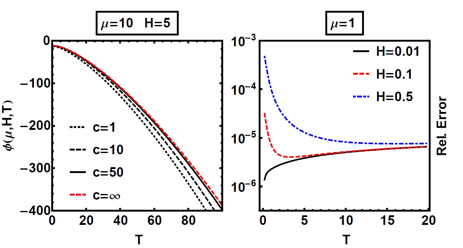
Figure 1: (Color online) Left panel. Temperature dependence of the grandcanonical potential calculated using Eq. (5) for $\mu=10\,,H=5$ and $c=1$ (dotted black line), $c=10$ (dashed black line) and $c=50$ (black line). In the limit of impenetrable particles we reproduce Takahashi’s result (8) (dashed red line). Right panel. Relative error $|\phi-\phi_{TBA}|/|\phi|$ with $\phi$ the grandcanonical potential given by Eq. (5) and $\phi_{TBA}$ calculated from the TBA equations (4) for $c=1,\mu=1$ and magnetic fields $H=\{0.01,0.1,0.5\}$. Grandcanonical potential per length and temperature in units of $\phi_{0}$ and $T_{0}$ uni .

$$\phi(\beta,\mu,H)=-\frac{1}{2\pi\beta}\int_{\mathbb{R}}\ln(1+a_{1}(k))+\ln(1+a_{2}(k))\,dk\,,$$ (5)

where $a_{1,2}(k)$ are auxiliary functions satisfying ($\varepsilon\rightarrow 0$)

$$\ln a_{1}(k) =-\beta(k^{2}-\mu-H)+\int_{\mathbb{R}}K_{2}^{F}(k-k^{\prime}-i\varepsilon)\ln(1+a_{2}(k^{\prime}))\,dk^{\prime}\,,$$ (6a)

$$\ln a_{2}(k) =-\beta(k^{2}-\mu+H)+\int_{\mathbb{R}}K_{1}^{F}(k-k^{\prime}+i\varepsilon)\ln(1+a_{1}(k^{\prime}))\,dk^{\prime}\,,$$ (6b)

and

$$K_{1}^{F}(k)=\frac{1}{2\pi}\frac{c}{k(k+ic)}\,,\ \ K_{2}^{F}(k)=\frac{1}{2\pi}\frac{c}{k(k-ic)}\,.$$ (7)

We would like to stress that this system of equation is exact and valid for all values of chemical potential, magnetic fields (including the balanced case $H=0$), positive coupling strengths and temperature. We also note that (6) differs from the result for the 2CBG derived in KP1 by dropping the diagonal terms.

In the left panel of Fig. 1 we present results for the temperature dependence of the grandcanonical potential of a system with $\mu=10$ and $H=5$ showing how for increasing values of the coupling strength $c=\{1,10,50\}$ we approach Takahashi’s result for impenetrable particles Tak1 ; Tbook

$$\phi_{\infty}(\beta,\mu,H)=-\frac{1}{2\pi\beta}\int_{\mathbb{R}}dk\,\ln\left(1+2\cosh(\beta H)e^{-\beta(k^{2}-\mu)}\right)\,.$$ (8)

A comparison between the grandcanonical potential for a system with $c=1$ and $\mu=1$ computed using Eq. (5) and the TBA equations (4) truncated at the $n=30$ level can be found in the right panel of Fig. 1. The results show almost perfect agreement which not only confirms the validity of our results but also supports the string hypothesis in the case of the repulsive Gaudin-Yang model.

In the noninteracting limit, $c\rightarrow 0$, using $\lim_{c\rightarrow 0}K_{2}^{F}(k-i\varepsilon)$ $=\lim_{c\rightarrow 0}K_{1}^{F}(k+i\varepsilon)=0$ it is easy to show that (5) reduces to $\phi_{0}(\beta,\mu,H)=\frac{1}{2\pi\beta}\int_{\mathbb{R}}\ln(1+e^{-\beta(k^{2}-\mu-H)})+\ln(1+e^{-\beta(k^{2}-\mu+H)})dk\,,$ which, as expected, is the result for free fermions in a magnetic field.

IV Thermodynamic properties of the homogeneous system

Despite being the first multi-component model solved by Bethe ansatz at zero and finite temperature our knowledge of the thermodynamic properties of the Gaudin-Yang model is still very limited. Fueled by the interest in the FFLO pairing phase the case of attractive interactions has received more attention Orso ; HLD ; HJLPAD ; BAD ; GYFBLL but even in this case a complete characterization of the thermodynamical properties is still lacking. The situation is even more dire in the repulsive case. The phase diagram at $T=0$ was derived by Colomé-Tatché ColTat and the low-temperature strong-coupling regime was investigated by Lee, Guan, Sakai and Batchelor in LGSB .

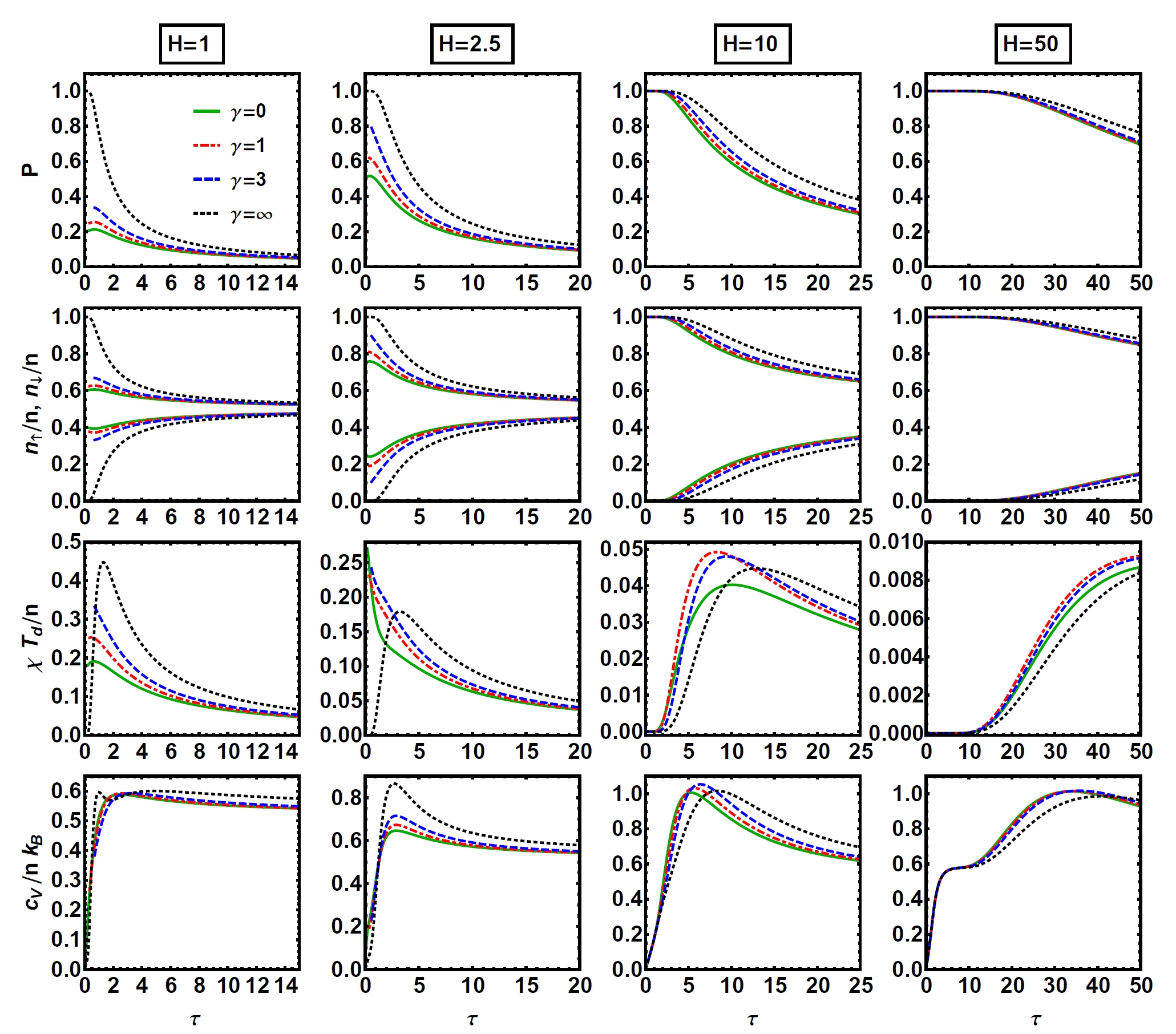
Figure 2: (Color online) Plots of the polarization (first row), densities of spin up and down particles (second row), susceptibility per length normalized by $n/T_{d}$ (third row) and specific heat per length normalized by $nk_{B}$ (bottom row) as functions of the reduced temperature $\tau=T/T_{d}=T/n^{2}$ for four values of the dimensionless coupling strength $\gamma=\{0,1,3,\infty\}$ and magnetic field $H=\{1,2.5,10,50\}$. The total density is fixed to $n=1$.

The main reason behind this information scarcity is the complexity of the TBA equations and other methods used in the investigation of thermodynamic properties, like lattice Monte-Carlo calculations, which require rather cumbersome numerical schemes in order to obtain accurate numerical data. In contrast, our equations (6), can be accurately and easily solved employing a simple iterative procedure with the convolutions treated using the Fast Fourier Transform and the convolution theorem. This scheme allows us to probe a wide region of the parameter space with the exception of the low polarization at low-temperatures regime ($H\ll\mu$ and $T\rightarrow 0$). This regime requires a more careful treatment of the NLIEs which will be deferred to a future publication.

In Fig. 2 we present for several values of the magnetic field the dependence on the reduced temperature $\tau=T/T_{d}=T/n^{2}$ of the densities $n_{\uparrow,\downarrow}$, polarization $P$, magnetic susceptibility $\chi$ and specific heat $c_{V}$ which can be derived from the grandcanonical potential (5)

$$n_{\uparrow,\downarrow}=-\frac{1}{2}\left(\frac{\partial\phi}{\partial\mu}\pm\frac{\partial\phi}{\partial H}\right)\,,\ P=\frac{n_{\uparrow}-n_{\downarrow}}{n_{\uparrow}+n_{\downarrow}}\,,\ \chi=-\left[\left(\frac{\partial^{2}\phi}{\partial H^{2}}\right)_{\mu}+\left(\frac{\partial n}{\partial H}\right)^{2}_{\mu}\left(\frac{\partial n}{\partial\mu}\right)^{-1}_{H}\right]\,,\ c_{V}=-T\left[\frac{\partial^{2}\phi}{\partial T^{2}}+\left(\frac{\partial n}{\partial T}\right)^{2}_{\mu}\left(\frac{\partial n}{\partial\mu}\right)_{T}^{-1}\right]\,.$$

At zero temperature and zero magnetic field the groundstate of the Gaudin-Yang model is balanced (number of particles with spin up is equal with the number of particles with spin down) and the excitation spectrum is gapless which means that switching a magnetic field the system will become partially polarized. The monotonously decreasing polarization of the system as a function of the reduced temperature in the presence of a constant magnetic field is presented in the upper panels of Fig. (2). We can also see that for a given $H$ and temperature the polarization is an increasing function of the interaction strength. For large values of the dimensionless coupling strength the system becomes paramagnetic as it can be seen from Eq. (8) which describes free fermions at chemical potential $\mu^{\prime}=\mu+\ln[2\cosh(\beta H)]$.

The magnetic susceptibility is finite everywhere except at $\gamma=\infty,$ $H=0$ and $T=0$. In this case we can see from Eq. (8)) that the magnetization is $M=n\tanh\left(H/T\right)$ and the susceptibility $\chi=n[1-\tanh^{2}\left(H/T\right)]/T$ diverges like $1/T$ at vanishing magnetic field. At low-temperatures and small magnetic fields $\chi$ presents a complex behavior as a function of $\gamma$. For $H=1$ the maximum susceptibility is obtained for $\gamma=\infty$ but already for $H=2.5$ the susceptibilities for $\gamma=\{0,1,3\}$ present more pronounced maxima at very low-temperatures while the maximum for $\chi(\gamma=\infty)$ moves at a higher temperature. For strong magnetic fields the susceptibility is zero at low-temperatures, presents a global maximum at a reduced temperature close to the value of the magnetic field and the dependence on the coupling strength becomes small. The specific heat is linear at low-temperatures and similar to the case of the susceptibility presents a maximum at a temperature $\tau\sim H$. A similar behavior was noticed by Klauser and Caux KC for the 2CBG but in our case the maxima are more pronounced for the same values of temperatures and magnetic field. At high temperatures the specific heat per particle approaches $1/2$, the value for the ideal gas. As a function of the coupling strength and for low values of the magnetic field the specific heat reaches its maximum for $\gamma=\infty$ but this is no longer true for strong magnetic fields where the dependence on $\gamma$ becomes less pronounced.

V Tan contact and local correlation functions

S. Tan Tan1 discovered that the momentum distribution of 3D fermions with zero range spin-independent interactions exhibits a universal $C/k^{4}$ behavior at large momenta (a similar relation for the Lieb-Liniger model was derived earlier by Olshanii and Dunjko OD ). The large momentum distribution is the same for both particle species and the constant $C$, called contact, is given by the probability that two particles of opposite spin are found at the same position in space. The contact also appears in Tan’s adiabatic theorem Tan1 which determines the change of the energy with respect to the interaction strength and a series of universal thermodynamic identities called Tan relations Tan1 (see also BP1 ; ZL ; WTC ; BZ ; VZM ; WC ). The analogues of Tan relations in 1D were derived by Barth and Zwerger BZ using the Operator Product Expansion of Wilson and Kadanoff Wils ; Kad . The contact is not only an important and valuable theoretical concept but is also experimentally measurable NNCS ; SGDJ ; KHLDMD ; KHHDHV2 ; KHDHHV1 ; SDPJ ; WMPCJ ; HLFHV .

In the case of the Gaudin-Yang model with the Hamiltonian (1) the contact is defined as BZ (remember $\hbar=2m=1$ and $c=-2/a_{1D}$ with $a_{1D}$ the scattering length)

$$C=\frac{4}{a^{2}_{1D}}\int dx\,\langle\Psi_{\uparrow}^{\dagger}(x)\Psi_{\downarrow}^{\dagger}(x)\Psi_{\downarrow}(x)\Psi_{\uparrow}(x)\rangle=c^{2}\int dx\,\langle\Psi_{\uparrow}^{\dagger}(x)\Psi_{\downarrow}^{\dagger}(x)\Psi_{\downarrow}(x)\Psi_{\uparrow}(x)\rangle\,,$$ (9)

where by $\langle\ \rangle$ we denote the zero or finite temperature expectation value. In our definition we can see that $C$ is an extensive variable and is closely related to the interaction energy $I=2c\int dx\,\langle\Psi_{\uparrow}^{\dagger}(x)\Psi_{\downarrow}^{\dagger}(x)\Psi_{\downarrow}(x)\Psi_{\uparrow}(x)\rangle$ and the local correlation function of opposite spins defined by

$$g_{\uparrow\downarrow}^{(2)}(x)=4\frac{\langle\Psi_{\uparrow}^{\dagger}(x)\Psi_{\downarrow}^{\dagger}(x)\Psi_{\downarrow}(x)\Psi_{\uparrow}(x)\rangle}{n(x)^{2}}=4\frac{\langle\Psi_{\uparrow}^{\dagger}(x)\Psi_{\downarrow}^{\dagger}(x)\Psi_{\downarrow}(x)\Psi_{\uparrow}(x)\rangle}{(n_{\uparrow}(x)+n_{\downarrow}(x))^{2}}\,.$$ (10)

A simple application of the Hellmann-Feynman theorem gives the 1D version of Tan’s adiabatic theorem BZ $\frac{dE}{da_{1D}}=\left\langle\frac{\partial\mathcal{H}_{GY}}{\partial a_{1D}}\right\rangle=C$ which expresses the variation of the total energy $E$ with respect to the scattering length.

The situation is considerably simplified in the homogeneous case $V(x)=0$. The local correlation function and density no longer depend on $x$ and we can introduce the contact and interaction energy per length

$$\mathcal{C}=\frac{c^{2}}{4}n^{2}g_{\uparrow\downarrow}^{(2)}(0)\,,\ \ \ \mathcal{I}=\frac{c}{2}n^{2}g_{\uparrow\downarrow}^{(2)}(0)\,.$$ (11)

Another application of the Hellmann-Feynman theorem allows us to obtain the local correlation function from the derivative of the grandcanonical potential per length with respect to the coupling strength $g_{\uparrow\downarrow}^{(2)}(0)=\frac{2}{n^{2}}\frac{\partial\phi}{\partial c}$. Noting that $\phi=-\ln\mathcal{Z}/(\beta L)$ with $\mathcal{Z}=Tr[e^{-\beta(\mathcal{H}_{GY}-\mu_{\uparrow}N_{\uparrow}-\mu_{\downarrow}N_{\downarrow})}]$ we have $\frac{\partial\phi}{\partial c}=Tr[\frac{\partial\mathcal{H}_{GY}}{\partial c}e^{-\beta(\mathcal{H}_{GY}-\mu_{\uparrow}N_{\uparrow}-\mu_{\downarrow}N_{\downarrow})}]/(L\mathcal{Z})$ $=2\langle\Psi_{\uparrow}^{\dagger}(0)\Psi_{\downarrow}^{\dagger}(0)\Psi_{\uparrow}(0)\Psi_{\downarrow}(0)\rangle_{T}$ which proves the identity. For the homogeneous system the pressure and total energy per length $\mathcal{E}$ satisfy the following Tan relation BZ $p=2\mathcal{E}-2\mathcal{C}/c$. We have checked numerically this relation and found perfect agreement providing an additional check for the validity of our NLIEs. Other analytical or numerical computations of the contact in 1D systems can be found in HJLPAD ; BAD ; RPLD ; YB ; ZWKGD ; DK ; BBF ; VM .

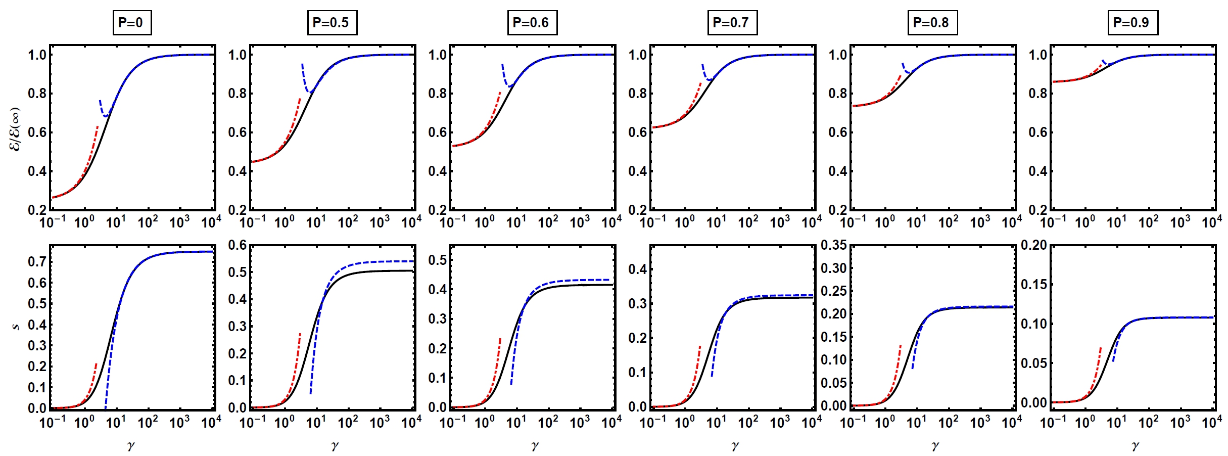
Figure 3: (Color online) Plots of the zero temperature energy density $\mathcal{E}$ at fixed polarization (upper panels black continuous line) in units of $\mathcal{E}(\infty)=n^{3}\pi^{2}/3$ and dimensionless contact $s=\mathcal{C}/k_{F}^{4}$ (lower panels black continuous line) with $k_{F}=\pi n/2$ as functions of the dimensionless coupling constant $\gamma.$ The dashed blue and dot-dashed red lines represent the asymptotic expansions in the strong and weak interaction limit given by Eqs. (13), (14) and (15). The results presented in the top row can be seen as complementing Fig. 1 of GM1 .

V.1 Results at T=0

At zero temperature the thermodynamic properties of the system can be extracted from the following system of Fredholm type integral equations Y1

$$\rho_{c}(k) =\frac{1}{2\pi}+\int_{-\lambda_{0}}^{\lambda_{0}}b_{1}(k-\lambda)\rho_{s}(\lambda)\,d\lambda\,$$ (12a)

$$\rho_{s}(\lambda) =\int_{-k_{0}}^{k_{0}}b_{1}(\lambda-k)\rho_{c}(k)\,dk-\int_{-\lambda_{0}}^{\lambda_{0}}b_{2}(\lambda-\mu)\rho_{s}(\mu)\,d\mu$$ (12b)

where $b_{m}(k)=mc/[2\pi[(mc)^{2}/4+k^{2}]].$ In Eqs. (12) $k_{0}$ and $\lambda_{0}$ are parameters which fix the values of the density of spin down particles and energy per length via $n=\int_{-k_{0}}^{k_{0}}\rho_{c}(k)\,dk\,,$ $n_{\downarrow}=\int_{-\lambda_{0}}^{\lambda_{0}}\rho_{s}(\lambda)\,d\lambda\,,$ and $\mathcal{E}=\int_{-k_{0}}^{k_{0}}k^{2}\rho_{c}(k)\,dk\,.$ The balanced system is characterized by $\lambda_{0}=\infty$ and the fully polarized system by $\lambda_{0}=0$. Even though in the general case an analytic solution of the system of equations (12) is not known, in certain limits approximate results can be derived. In the strong interaction limit ($\gamma\gg 1$) Guan and Ma GM1 obtained (the leading order term was derived in Fuchs ; BCS2 )

$$\mathcal{E}=\left\{\begin{array}[]{ll}\frac{n^{3}\pi^{2}}{3}\left[1-\frac{4\ln 2}{\gamma}+\frac{12(\ln 2)^{2}}{\gamma^{2}}-\frac{32(\ln 2)^{3}}{\gamma^{3}}+\frac{\pi^{2}\zeta(3)}{\gamma^{3}}\right]\,,\ \ P=0\,,\\ \frac{n^{3}\pi^{2}}{3}\left[1-\frac{4(1-P)}{\gamma}+\frac{12(1-P)^{2}}{\gamma^{2}}-\frac{32(1-P)^{3}}{\gamma^{3}}+\frac{16\pi^{2}(1-P)}{5\gamma^{3}}\right]\,,\ \ P\geq 0.5\,,\end{array}\right.$$ (13)

with $\zeta(z)$ the Riemann function, and in the weak interaction limit $(\gamma\ll 1)$

$$\mathcal{E}=\frac{n^{3}\pi^{2}(1-P)^{3}}{24}+\frac{n^{3}\pi^{2}(1+P)^{3}}{24}+\gamma\frac{n^{3}(1-P^{2})}{2}\,.$$ (14)

It should be emphasized that Eqs. (13) and (14) are not exact. They represent numerical approximations which are valid only in the Tonks-Girardeau ($\gamma\gg 1$) and weak interaction ($\gamma\ll 1$) regimes. Using Tan’s adiabatic theorem (see above) the local correlation function of opposite spins, contact and interaction energy can be computed as

$$g_{\uparrow,\downarrow}^{(2)}(0)=\frac{2}{n^{3}}\frac{d\mathcal{E}}{d\gamma}\,,\ \ \mathcal{C}=\frac{n}{2}\gamma^{2}\frac{d\mathcal{E}}{d\gamma}\,,\ \ \ \mathcal{I}=\gamma\frac{d\mathcal{E}}{d\gamma}\,.$$ (15)

In the following it will be preferable to work with the dimensionless contact density defined as $s=\mathcal{C}/k_{F}^{4}$ with $k_{F}=\pi n/2$.

In Fig. 3 we present results for the zero temperature energy and dimensionless contact as functions of the coupling constant obtained from the numerical integration of Eqs. (12) and the asymptotic expansions (13) and (14). In the balanced case ($P=0$) the asymptotic expansions for energy and contact represent a good approximation in the weak and strong interacting regime but in the case of imbalanced systems ($P\neq 0$) the results derived from Eq. (13) for the strongly interacting regime become more accurate as the polarization approaches one. The contact is a monotonously increasing function of $\gamma$ and in the Tonks-Girardeau limit ($\gamma\rightarrow\infty$) approaches asymptotically a finite value. As a function of the polarization $s$ reaches a maximum for $P=0$ and is zero for the fully polarized system. For the balanced system in the strongly interacting regime, using (13) and (15) we obtain

$$s(\gamma,P=0)=\frac{8}{3\pi^{2}}\left[4\ln 2-\frac{24(\ln 2)^{2}}{\gamma}+\frac{96(\ln 2)^{3}}{\gamma^{2}}-\frac{3\pi^{2}\zeta(3)}{\gamma^{2}}\right]\,,\ \gamma\gg 1\,,$$ (16)

with $s(\infty,P=0)=32\ln 2/(3\pi^{2})$ a result which was first obtained in BZ .

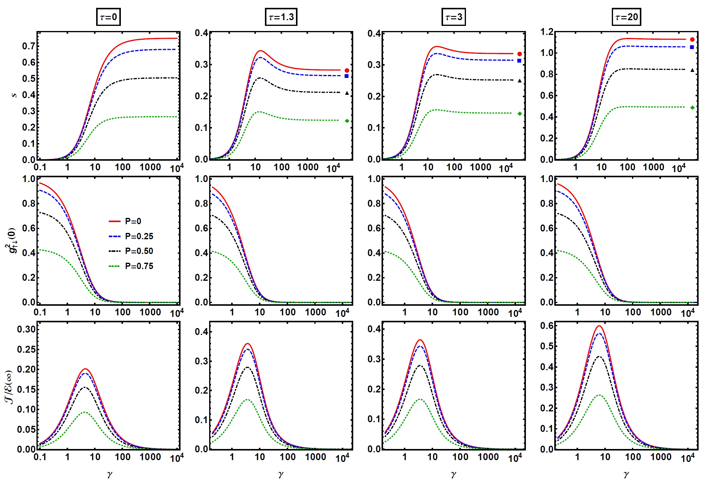
Figure 4: (Color online) Plots of the dimensionless contact $s$ (upper panels) local correlation function of opposite spins $g_{\uparrow\downarrow}^{(2)}(0)$ (middle panels) and interaction energy $\mathcal{I}$ (lower panels) as functions of the dimensionless coupling constant $\gamma$ for $\tau=\{0,1.3,3,20\}$ and fixed polarization $P=0$ (red line), $P=0.25$ (blue dashed line), $P=0.5$ (black dot-dashed line) and $P=0.75$ (green dotted line). The red disks, blue squares, black triangles and green diamonds represent the values of the dimensionless contact $s(\gamma=\infty)$ computed from the momentum distribution derived from the Fredholm determinants (17) for $P=\{0,0.25,0.5,0.75\}$. The total density is fixed to $n=1/2$.

V.2 Results at finite temperature

As we have mentioned before at finite temperature analytical results are restricted to the low-temperature strong-coupling regime LGSB and therefore we will have to rely on numerical solutions of the NLIEs (6). In Fig. 4 we present the dependence on the interaction strength of the dimensionless contact, local correlation function and interaction energy for fixed polarization and several values of the reduced temperature.

An interesting feature revealed by our data is that the contact at low and intermediate temperatures (see upper panels of Fig. 4) presents a local maximum (for any value of the polarization) which does not appear at $\tau=0$ and gets suppressed at high temperatures. In the Tonks-Girardeau regime the contact approaches a finite value for all values of $\tau$. Remembering that the contact governs the tail of the momentum distribution ($\tilde{n}(k)\sim\mathcal{C}/k^{4}$ for $k\rightarrow\infty$) this means that at $\tau=0$ and fixed polarization (or magnetic field) the width of the momentum distribution increases monotonically with $\gamma$ reaching its maximum at $\gamma=\infty.$ In contrast, at low and intermediate temperatures the width of the momentum distribution reaches a maximum at a finite value of the coupling strength and then becomes narrower as $\gamma\rightarrow\infty.$ This reconstruction of the momentum distribution as a function of the strength of the interaction should be in principle experimentally accessible.

As shown in the middle panels of Fig. 4 the local correlation function which quantifies the probability that two particles of opposite spin occupy the same point in space is a monotonically decreasing function of $\gamma$ with a maximum in the noninteracting limit ($g_{\uparrow\downarrow}^{(2)}(0)=1$ for $P=\gamma=0$ and all $\tau$). In the strongly interacting limit $g_{\uparrow\downarrow}^{(2)}(0)$ drops to zero like $1/\gamma^{2}$. For a fixed value of $\gamma$ as a function of the polarization the local correlator is maximal in the balanced system and vanishes in the fully polarized case. The interaction energy (bottom row Fig. 4) exhibits a local maximum at zero and finite temperature and vanishes for $\gamma\rightarrow\infty$. This is due to the fact that in the strong interaction limit the short-range repulsive interaction acts as an effective Pauli exclusion principle also between fermions of opposite spins BZ . As expected, the interaction energy is largest for the $P=0$ case and it is zero for the fully polarized system.

An alternative way of deriving the contact requires the analytical or numerical computation of the momentum distribution which is the Fourier transform of the static Green’s function i.e., $\tilde{n}(k)=\int_{-\infty}^{+\infty}e^{-ikx}\langle\Psi_{\uparrow}^{\dagger}(x)\Psi_{\uparrow}(0)\rangle_{\mu,H,T}\,dx.$ In the general case this is an almost hopeless task due to the fact that our knowledge of the correlators is still rather limited BL ; Ber ; ISLL1 ; IP1 ; GIKP ; GIK ; GKa . However, in the impenetrable case we can use the Fredholm determinant representations derived by Izergin and Pronko IP1 which have the advantage of being extremely easy to implement numerically using the method presented in Bor . In our case the Green’s functions have the following representation IP1

$$\langle\Psi_{\uparrow}^{\dagger}(x)\Psi_{\uparrow}(0)\rangle_{\mu,H,T}=\mbox{\tt det}\left(\hat{\textsf{I}}+\frac{e^{2H/T}}{2}\ \hat{\textsf{V}}+\hat{\textsf{R}}\right)-\mbox{\tt det}\left(\hat{\textsf{I}}+\frac{e^{2H/T}}{2}\ \hat{\textsf{V}}\right)\,,\$$ (17)

where the integral operators $\hat{\textsf{V}}$ and $\hat{\textsf{R}}$ act on an arbitrary function like $(\hat{\textsf{V}}f)(\lambda)=\int_{-\infty}^{+\infty}\textsf{V}(\lambda,\mu)f(\mu)\,d\mu$ and $(\hat{\textsf{R}}f)(\lambda)=\int_{-\infty}^{+\infty}\textsf{R}(\lambda,\mu)f(\mu)\,d\mu$ with kernels

$$\textsf{V}(\lambda,\mu)=-\,\sqrt{\theta(\lambda)}\,\frac{2\sin\left(|x|\frac{\lambda-\mu}{2}\right)}{\pi(\lambda-\mu)}\,\sqrt{\theta(\mu)}\,,\ \ \textsf{R}(\lambda,\mu)=-\,\sqrt{\theta(\lambda)}\,\frac{e^{-ix\frac{\lambda+\mu}{2}}}{2\pi}\,\sqrt{\theta(\mu)}\,,$$ (18)

and $\theta(\lambda)=e^{-H/T}/(2\cosh(H/T)+e^{(\lambda^{2}-\mu)/T})$ is the Fermi weight. In addition we have $\langle\Psi_{\downarrow}^{\dagger}(x)\Psi_{\downarrow}(0)\rangle_{\mu,H,T}=\langle\Psi_{\uparrow}^{\dagger}(x)\Psi_{\uparrow}(0)\rangle_{\mu,-H,T}\,.$ The results for the contact obtained from the large $k$ analysis of the Fourier transform of (17) are presented in the $\tau=\{1.3,3,20\}$ panels of Fig. 4 as red disks ($P=0$), blue squares ($P=0.25$), black triangles ($P=0.5$) and green diamonds ($P=0.75$) and they are in perfect agreement with the results derived from the NLIEs.

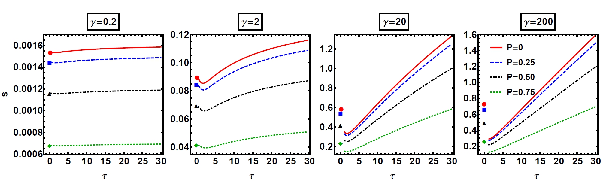
Figure 5: (Color online) Reduced temperature dependence of the dimensionless contact $s$ for $\gamma=\{0.2,2,20,200\}$ and fixed polarization $P=0$ (red line), $P=0.25$ (blue dashed line), $P=0.5$ (black dot-dashed line) and $P=0.75$ (green dotted line). The red disks, blue squares, black triangles and green diamonds represent the values of the dimensionless contact $s(\tau=0)$ computed from the integral equations (12) for $P=\{0,0.25,0.5,0.75\}$.

The temperature dependence of the contact shown in Fig. 5 reveals another interesting phenomenon (in Fig. 5 the values of the contact at $\tau=0$ were computed from the integral equations (12) and for $\tau>0$ from the NLIEs (6)). For weak interactions the dependence of $s$ on temperature is very small, but as we increase the coupling strength, the contact develops a local minimum which becomes very pronounced in the Tonks-Girardeau limit. The nonmonotonic behavior is present for all polarizations and the temperature interval in which it manifests itself shrinks as the value of $\gamma$ increases. Outside of this temperature interval and for strong interactions the contact presents a linear dependence on the reduced temperature for all values of $P.$ The nonmonotonic behavior of the contact implies that the shape of the momentum distribution of the strongly repulsive Gaudin-Yang model suffers an abrupt change in a very small interval of temperature. This reconstruction of the distribution is also counterintuitive because as the temperature increases the distribution becomes narrower and not wider as one would expect from a system of weakly interacting or free particles. However, one should not forget that in this case we are dealing with a strongly interacting system where this type of picture is not correct.

This crossover of the momentum distribution was first discovered by Cheianov, Smith and Zvonarev in CSZ for the balanced system and signals the transition from the Tomonaga-Luttinger liquid phase to the incoherent spin Luttinger liquid regime. Our results show that a similar crossover is present also in the imbalanced case and it might be possible to be detected even for moderate values of the coupling strength. Compared with the single-component case in the two-component system there are two temperature scales $T_{F}=\pi^{2}n^{2}$ and $T_{0}=T_{F}/\gamma$ (remember $\hbar=2m=k_{B}=1$) which define two different quantum regimes: $T<T_{0}$ characterized by the Tomonaga-Luttinger liquid theory and $T_{0}\ll T\ll T_{F}$ in which the incoherent spin Luttinger theory is applicable. The two temperature scales are well separated in the strong coupling limit and for $T_{0}\ll T\ll T_{F}$ the charge degrees of freedom are effectively frozen while the spin degrees of freedom are strongly “disordered”. It is important to note that in the computation of the correlation functions the limits $c\rightarrow 0$ and $T\rightarrow 0$ do not commute ISLL1 . The determinant representation (17) has been derived by taking the $c\rightarrow\infty$ limit in the wavefunctions followed by the summation of form factors at finite temperature. If we take the limit $T\rightarrow 0$ in (17) and compute the dimensionless contact from the tail of the momentum distribution we obtain $s(\gamma=\infty,P=0)_{T>T_{0}}=0.270$ which is considerably smaller than $s(\gamma=\infty,P=0)_{T<T_{0}}=32\ln 2/(3\pi^{2})=0.749...$ (see Eq. (16)) obtained from the integral equations at zero temperature (Eqs. 12). The momentum crossover for the balanced impenetrable system is presented in Fig. 1 of CSZ .

VI Density profiles at finite temperature

In most experiments the system is subjected to a harmonic potential $V(x)=m\omega^{2}x^{2}/2$, a situation in which the Hamiltonian (1) is no longer exactly solvable. However, for slowly varying potentials we can apply the Local Density Approximation (LDA) and the $V(x)=0$ solution to obtain reasonably accurate data for the trapped system. Under LDA each point in the trap can be seen as a locally homogeneous system with

$$\mu(x)=\mu(0)-V(x)=\mu(0)-m\omega^{2}x^{2}/2\,,\ \ \ H(x)=H(0)\,,$$ (19)

where $\mu(0)$ and $H(0)$ are the chemical potential and magnetic field in the center of the trap. An immediate consequence of (19) is that the density along the trap is monotonously decreasing and at zero temperature vanishes at a distance $R_{TF}$ from the center of the trap where $R_{TF}$ is called the Thomas-Fermi radius and is determined by $\mu(0)-m\omega^{2}R_{TF}^{2}/2=0$. An inhomogeneous system can be characterized by three parameters: the dimensionless coupling strength $\gamma(0)=c/n(0)$, the polarization $P(0)=(n_{\uparrow}(0)-n_{\downarrow}(0))/n(0)$ and the reduced temperature $\tau(0)=T/n^{2}(0)$ all evaluated at the center of the trap.

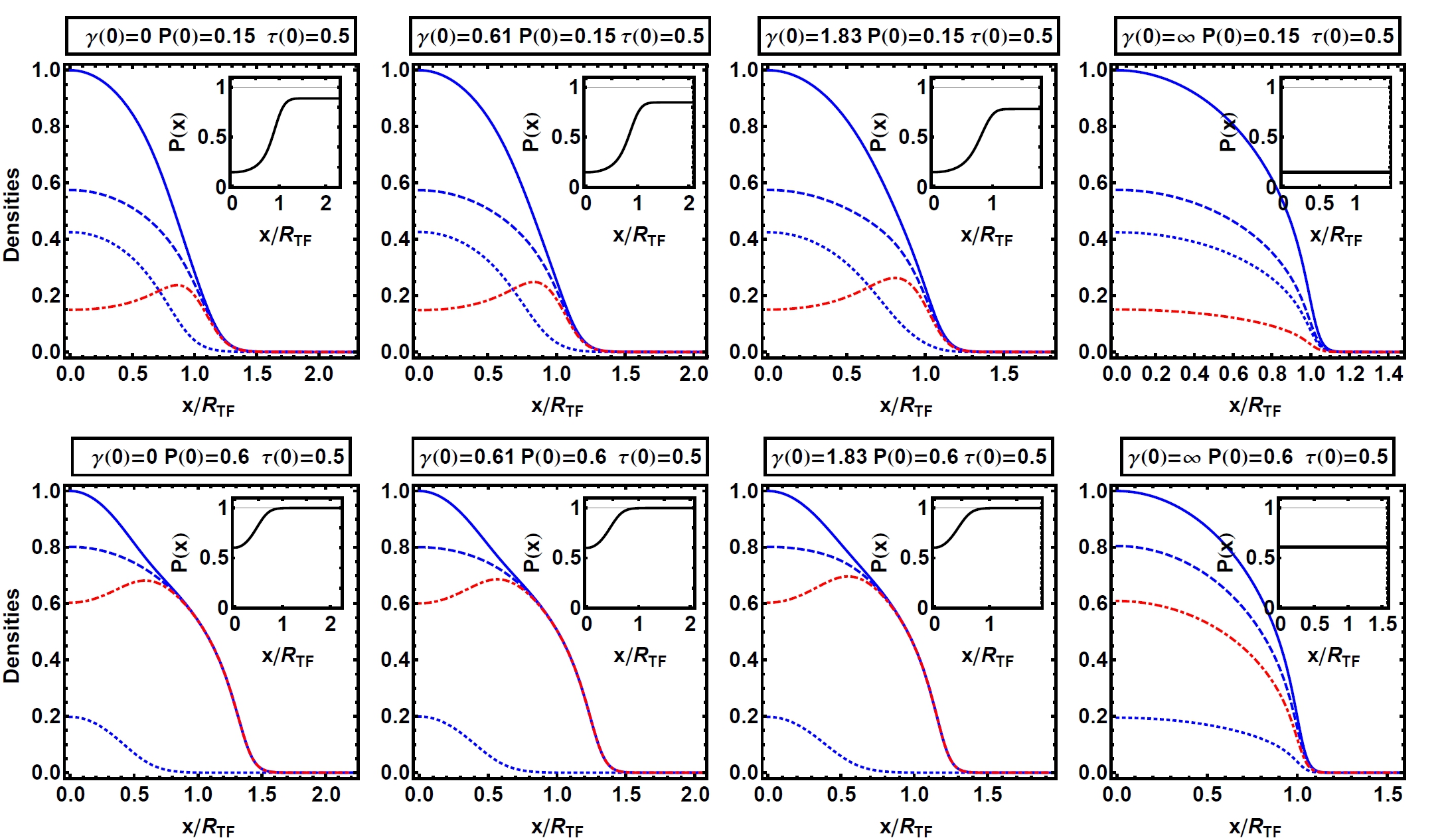
Figure 6: (Color online) Plots of the normalized total density $n(x)/n(0)$ (blue continuous line), normalized density of up spins $n_{\uparrow}(x)/n(0)$ (blue dashed line), normalized density of down spins $n_{\downarrow}(x)/n(0)$ (blue dotted line) and their difference $(n_{\uparrow}(x)-n_{\downarrow}(x))/n(0)$ (red dot-dashed line) for an inhomogeneous Gaudin-Yang model with $\tau(0)=0.5$ and polarizations $P(0)=0.15$ (upper panels) and $P(0)=0.6$ (lower panels). The insets depict the variation of the polarization $P(x)=(n_{\uparrow}(x)-n_{\downarrow}(x))/(n_{\uparrow}(x)+n_{\downarrow}(x))$ in the trap. For all values of the coupling strength $\gamma(0)=\{0,0.61,1.83,\infty\}$ the total density in the center of the trap is $n(0)=\sqrt{24}$.

The density profiles at $T=0$ were computed in ColTat and it was noticed that for all $P(0)\in(0,1)$ they present a two shell structure: an imbalanced mixture of spin up and down fermions in the center and fully polarized wings. At finite temperature the situation becomes more complex as it can be seen in Fig. 6 where we present the density profiles at $\tau(0)=0.5$ for different values of the coupling strength and two polarizations. For $P(0)=0.15$ and $\tau(0)=0.5$ the entire system is in the mixed phase for all values of $\gamma(0)$ (the density $n(0)=\sqrt{24}$ is the same in all cases presented) even though the polarization along the trap increases away from the center. The double shell structure appears only for values of the center polarization above a critical value which is a monotonic increasing function of $\gamma(0)$ and temperature (see the lower panels of Fig. 6). At high temperatures the entire system will be found only in the mixed phase irrespective of the value of $\gamma(0)$ and $P(0)$.

VII The Gaudin-Yang model as the continuum limit of the Perk-Schultz spin chain with $(-++)$ grading

The derivation of Eqs. (5) and (6) is performed in three steps. First, we identify a lattice embedding of the Gaudin-Yang model for which the quantum transfer matrix method MS ; K1 can be employed. The need for this lattice model stems from the fact that the quantum transfer matrix method, which has the advantage of producing a finite number of NLIEs for the thermodynamics of the system, can be defined only for discrete systems. In the second step we calculate the free energy of this lattice model from the largest eigenvalue of the QTM. Finally, the thermodynamics of the continuum model is obtained by performing the scaling limit in the result for the lattice model.

As in the case of the two-component Bose gas KP1 ; KP2 the appropriate lattice model is the $q=3$ critical Perk-Schultz spin chain dVL ; L

$$\cal{H}_{PS} =J\varepsilon_{1}\sum_{j=1}^{L}\left(\cos\gamma\sum_{a=1}^{3}\varepsilon_{a}\,e_{aa}^{(j)}e_{aa}^{(j+1)}+\sum_{\begin{subarray}{c}a,b=1\\ a\neq b\end{subarray}}^{3}e_{ab}^{(j)}e_{ba}^{(j+1)}+i\sin\gamma\sum_{\begin{subarray}{c}a,b=1\\ a\neq b\end{subarray}}^{3}\mbox{sign}(a-b)e_{aa}^{(j)}e_{bb}^{(j+1)}\right)-\sum_{j=1}^{L}\sum_{a=1}^{3}h_{a}e_{aa}^{(j)}\,,$$ (20)

where $J>0$ is the coupling strength, $L$ is the number of lattice sites, $\gamma\in[0,\pi]$ is the anisotropy, $h_{1},h_{2},h_{3}$ are chemical potentials and $\varepsilon_{1},\varepsilon_{2},\varepsilon_{3},\,(\varepsilon_{i}\in\{\pm 1\})$ are the grading parameters. Also $e^{(j)}_{ab}=\mathbb{I}_{3}^{\otimes j-1}\otimes e_{ab}\otimes\mathbb{I}_{3}^{\otimes L-j}\,,$ with $e_{ab}$ and $\mathbb{I}_{3}$ the canonical basis and the unit matrix in the space of $3$-by-$3$ matrices. If in the case of the 2CBG we considered the grading $(\varepsilon_{1},\varepsilon_{2},\varepsilon_{3})=(---),$ for the Gaudin-Yang model the relevant grading is $(\varepsilon_{1},\varepsilon_{2},\varepsilon_{3})=(-++)$. The energy spectrum of the spin chain is (see Appendix A)

$$E_{PS}=\sum_{j=1}^{M}e_{0}(v^{(1)}_{j})+M_{1}(h_{2}-h_{3})+E_{0}\,,\ \ \ e_{0}(v)=J\frac{\sin^{2}\gamma}{\sin(v-\gamma)\sin v}+h_{1}-h_{2}\,,\ \ \ E_{0}=JL\cos\gamma-h_{1}L\,,$$ (21)

with the Bethe ansatz equations

$$\left(\frac{\sin(\gamma-v_{s}^{(1)})}{\sin v_{s}^{(1)}}\right)^{L}=(-1)^{M-1}\prod_{p=1}^{M_{1}}\frac{\sin(v_{s}^{(1)}-v_{p}^{(2)}-\gamma)}{\sin(v_{s}^{(1)}-v_{p}^{(2)})}\,,\ \ \ s=1,\cdots,M\,,$$ (22a)

$$\prod_{j=1}^{M}\frac{\sin(v_{l}^{(2)}-v_{j}^{(1)}+\gamma)}{\sin(v_{l}^{(2)}-v_{j}^{(1)})}=\prod_{\begin{subarray}{c}p=1\\ p\neq l\end{subarray}}^{M_{1}}\frac{\sin(v_{l}^{(2)}-v_{p}^{(2)}+\gamma)}{\sin(v_{l}^{(2)}-v_{p}^{(2)}-\gamma)}\,,\ \ \ l=1,\cdots,M_{1}\,.$$ (22b)

In order to prove that the Perk-Schultz spin chain with the $(-++)$ grading is the lattice embedding of the 2CFG we are going to show that the spectrum and Bethe equations of the continuum model (2), (3) can be obtained in a scaling limit from the lattice analogues (21), (22). We start with the Bethe ansatz equations. Performing the transformation $v_{s}^{(1)}\rightarrow i\delta k_{s}^{(1)}/\epsilon+\gamma/2\,,$ and $v_{l}^{(2)}\rightarrow i\delta k_{l}^{(1)}/\epsilon+\pi/2$ with $\delta$ the lattice constant and $\epsilon\rightarrow 0$ a small parameter, Eqs. (22) take the form

$$\left((-)\frac{\sinh(\delta k_{s}^{(1)}/\epsilon-i\gamma/2)}{\sinh(\delta k_{s}^{(1)}/\epsilon+i\gamma/2)}\right)^{L}=(-1)^{M-1}\prod_{p=1}^{M_{1}}\frac{\cosh(\delta k_{s}^{(1)}/\epsilon-\delta k_{p}^{(2)}/\epsilon-i\gamma/2)}{\cosh(\delta k_{s}^{(1)}/\epsilon-\delta k_{p}^{(2)}/\epsilon+i\gamma/2)}\,,$$

$$\prod_{j=1}^{M}\frac{\cosh(\delta k_{l}^{(2)}/\epsilon-\delta k_{j}^{(1)}/\epsilon-i\gamma/2)}{\cosh(\delta k_{l}^{(2)}/\epsilon-\delta k_{j}^{(1)}/\epsilon+i\gamma/2)}=\prod_{\begin{subarray}{c}p=1\\ p\neq l\end{subarray}}^{M_{1}}\frac{\sinh(\delta k_{l}^{(2)}/\epsilon-\delta k_{p}^{(2)}/\epsilon-i\gamma)}{\sinh(\delta k_{l}^{(2)}/\epsilon-\delta k_{p}^{(2)}/\epsilon+i\gamma)}\,.$$

Considering $\gamma=\pi-\epsilon$ we obtain

$$\left(\frac{\cosh(\delta k_{s}^{(1)}/\epsilon+i\epsilon/2)}{\cosh(\delta k_{s}^{(1)}/\epsilon-i\epsilon/2)}\right)^{L}=(-1)^{M-1}\prod_{p=1}^{M_{1}}(-)\frac{\sinh(\delta k_{s}^{(1)}/\epsilon-\delta k_{p}^{(2)}/\epsilon+i\epsilon/2)}{\sinh(\delta k_{s}^{(1)}/\epsilon-\delta k_{p}^{(2)}/\epsilon-i\epsilon/2)}\,,$$ (23a)

$$\prod_{j=1}^{M}(-)\frac{\sinh(\delta k_{l}^{(2)}/\epsilon-\delta k_{j}^{(1)}/\epsilon+i\epsilon/2)}{\sinh(\delta k_{l}^{(2)}/\epsilon-\delta k_{j}^{(1)}/\epsilon-i\epsilon/2)}=\prod_{\begin{subarray}{c}p=1\\ p\neq l\end{subarray}}^{M_{1}}\frac{\sinh(\delta k_{l}^{(2)}/\epsilon-\delta k_{p}^{(2)}/\epsilon+i\epsilon)}{\sinh(\delta k_{l}^{(2)}/\epsilon-\delta k_{p}^{(2)}/\epsilon-i\epsilon)}\,.$$ (23b)

If we take the limits $L\rightarrow\infty,\delta\rightarrow 0$, $(L\sim\mathcal{O}(1/\epsilon^{2})\,,\delta\sim\mathcal{O}(\epsilon^{2}))$ such that $L\delta=L_{F}$, $c=\epsilon^{2}/\delta$, identifying $M_{1}$ with $M_{\downarrow}$ and using

$$\frac{\cosh(\delta k_{s}^{(1)}/\epsilon+i\epsilon/2)}{\cosh(\delta k_{s}^{(1)}/\epsilon-i\epsilon/2)}\sim\frac{1+ik_{s}^{(1)}\delta/2}{1-ik_{s}^{(1)}\delta/2}$$

we see that for $M$ even and $M_{1}$ odd Eqs. (23) transform in the Bethe equations of the Gaudin-Yang model (3).

Under this set of transformations the energy spectrum becomes

$$\beta(E_{PS}-E_{0})=\sum_{j=1}^{M}\beta\left[J\delta^{2}(k_{j}^{(1)})^{2}-J\epsilon^{2}-J\epsilon^{4}/4\right]+\beta(h_{1}-h_{2})M+\beta(h_{2}-h_{3})M_{1}+\mathcal{O}(\epsilon^{6})\,.$$ (24)

If we denote by $\bar{\beta}$ the inverse temperature of the continuum model and consider $\beta=\bar{\beta}/\delta^{2}$, $J=1,$ $h_{1},h_{2},h_{3}\rightarrow 0$ $(h_{1}\sim\mathcal{O}(\epsilon^{2})\,,h_{2},h_{3}\sim\mathcal{O}(\epsilon^{4}))$ such that $J\epsilon^{2}/\delta^{2}-h_{1}/\delta^{2}$ is finite we have

$$e^{\beta E_{0}}Z(h_{1},h_{2},h_{3},\beta)\rightarrow\mathcal{Z}(\mu,H,\bar{\beta})\,.$$ (25)

where $Z(h_{1},h_{2},h_{3},\beta)$ is the canonical partition function of the spin chain and $\mathcal{Z}(\mu,H,\bar{\beta})$ is the grandcanonical partition function of the Gaudin-Yang model. Therefore, we have showed that by performing the scaling limit presented above (the spectral parameter $v\rightarrow i\delta k/\epsilon$) the thermodynamics of the 2CFG can be derived from the similar result for the low-T critical Perk-Schultz spin chain with $(-++)$ grading. It should be noted that the scaling limit presented here is the same as the one employed in the 2CBG case (see Table I of KP2 ) the only difference being the grading.

VIII Free energy of the $(-++)$ Perk-Schultz spin chain

The importance of the quantum transfer matrix MS ; Koma ; SI1 ; K1 ; K2 in the study of integrable lattice models resides in the fact that not only the free energy of the model is related to the largest eigenvalue of the QTM but also various correlation lengths can be derived from the spectrum of the next-largest eigenvalues. The definition of the QTM for the Perk-Schultz spin chain in the algebraic Bethe ansatz framework can be found in KP2 . The interested reader can find pedagogical introductions in the subject in K3 ; GKS1 ; GSuz .

The largest eigenvalue of the quantum transfer matrix (see Appendix A), which will be denoted by $\Lambda_{0}(v)$, is found in the $(N/2,N/2)$-sector of the spectrum which means that $m=n=N/2$ in Eqs. (49) and (50). $\Lambda_{0}(v)$ is related to the free energy per lattice site of the Perk-Schultz spin chain via the relation $f(\beta,h_{1},h_{2},h_{3})=-(\ln\Lambda_{0}(0))/\beta$. In the following it will be useful to introduce the notations $\phi_{\pm}(v)=\left(\sinh(v\pm iu)/\sin\gamma\right)^{N/2}$ with $u=J\sin\gamma\beta/N$ where $N$ is the Trotter number and $q_{0}(v)=\phi_{-}(v),\ q_{j}(v)=\prod_{r=1}^{N/2}\sinh(v-v_{r}^{(j)}),\ j=1,2,\ q_{3}(v)=\phi_{+}(v).$ Changing the spectral parameter $v\rightarrow iv$ and considering $N\in 4\mathbb{N}$, the expression for the largest eigenvalue of the QTM (49) can be written as (see the last remark of Appendix A)

$$\Lambda_{0}(v)=\lambda_{1}(v)+\lambda_{2}(v)+\lambda_{3}(v)\,,\ \ \ \lambda_{j}(v)=\phi_{-}(v)\phi_{+}(v)\frac{q_{j-1}(v-i\tilde{\varepsilon}_{j}\gamma)}{q_{j-1}(v)}\frac{q_{j}(v+i\tilde{\varepsilon}_{j}\gamma)}{q_{j}(v)}e^{\beta\tilde{h}_{j}}\,,$$ (26)

with $(\tilde{\varepsilon}_{1},\tilde{\varepsilon}_{2},\tilde{\varepsilon}_{3})=$ $(+-+)$ and $(\tilde{h}_{1},\tilde{h}_{2},\tilde{h}_{3})=(h_{3},h_{1},h_{2})$. In this notation the BAEs (50) take the form $\ \lambda_{j}(v^{(j)}_{r})/\lambda_{j+1}(v^{(j)}_{r})=-1\,,\ r=1,\cdots,N/2\,,(j=1,2).$

VIII.1 Nonlinear integral equations for the auxiliary functions

The derivation of the nonlinear integral equations and integral expression for the largest eigenvalue of the QTM in the Gaudin-Yang model is very similar with the one presented in KP2 for the two-component Bose gas. For this reason, below we will not be as explicit as in the 2CBG case but we will highlight the particular features introduced by the fermionic model.

We introduce two auxiliary functions periodic of period $i\pi$ defined by

$$\mathfrak{a}_{1}(v) =\frac{\lambda_{1}(v)}{\lambda_{2}(v)}=\frac{\phi_{-}(v-i\gamma)}{\phi_{-}(v)}\frac{q_{2}(v)}{q_{2}(v-i\gamma)}e^{\beta(h_{3}-h_{1})}\,,$$ (27a)

$$\mathfrak{a}_{2}(v) =\frac{\lambda_{3}(v)}{\lambda_{2}(v)}=\frac{\phi_{+}(v+i\gamma)}{\phi_{+}(v)}\frac{q_{1}(v)}{q_{1}(v+i\gamma)}e^{\beta(h_{2}-h_{1})}\,.$$ (27b)

The equation $\mathfrak{a}_{1,2}(v)=-1$ has $N$ solutions and contains as a subset the $N/2$ Bethe roots (see the remark after Eq. (26)) which will be denoted by $\{v_{j}^{(1,2)}\}_{j=1}^{N/2}$. The additional $N/2$ solutions are called holes and will be denoted by $\{v_{j}^{\prime(1,2)}\}_{j=1}^{N/2}.$ We will first focus on the case when $\gamma\in(0,\pi/2)$ and we are going to assume that the Bethe roots and holes for the largest eigenvalue of the QTM are distributed in the complex plane as in Fig.7.

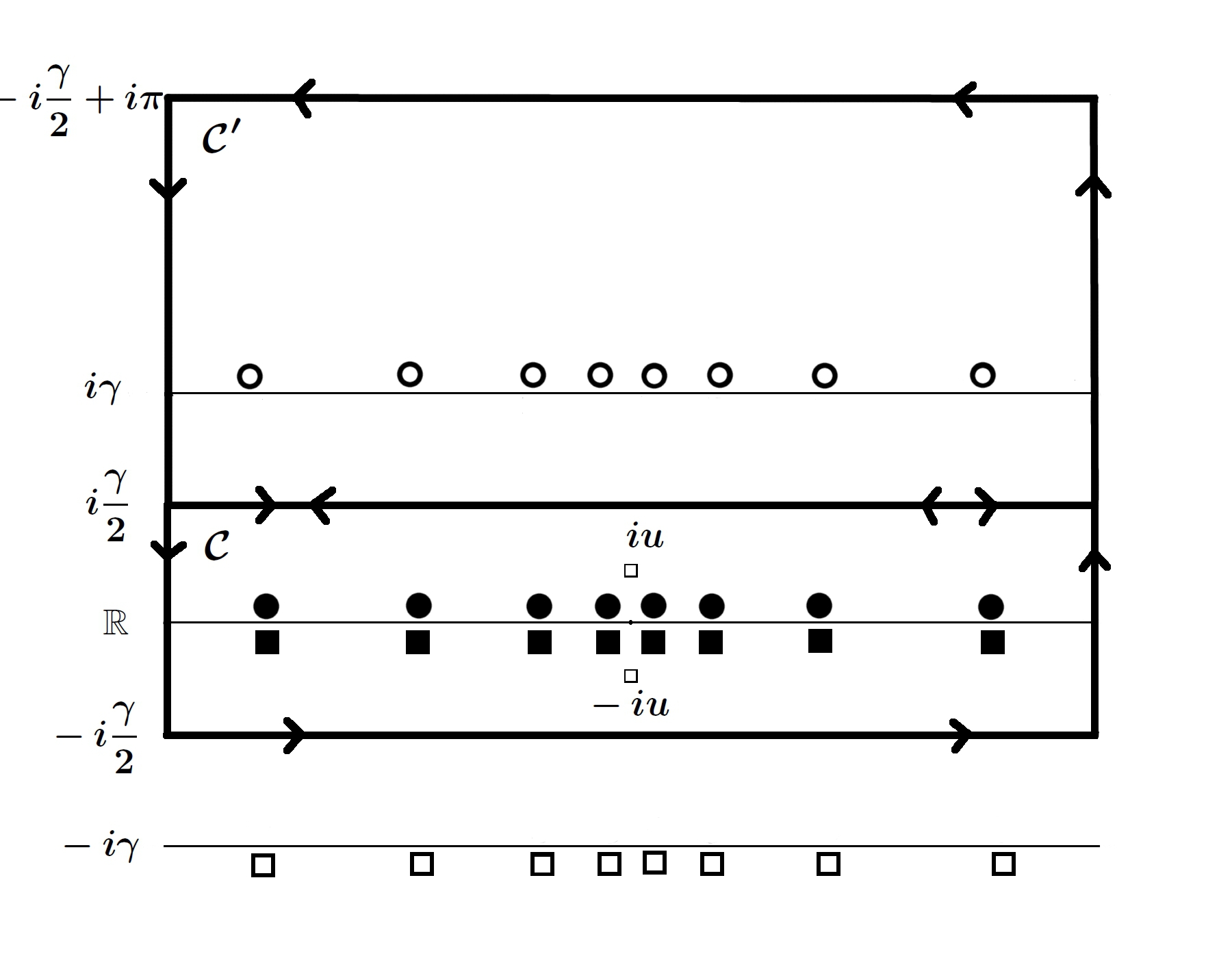
Figure 7: Relevant contours and distribution of Bethe roots $\{v^{(1)}_{i}\}\,,\{v^{(2)}_{j}\}$ ($\bullet,\blacksquare$) and holes $\{v^{\prime(1)}_{i}\}\,,\{v^{\prime(2)}_{j}\}$ ($\circ,\square$) for the largest eigenvalue ($\gamma\in(0,\pi/2)$). The upper and lower edges of $\mathcal{C}$ are parallel with the real axis and intersect the imaginary axis at $\pm i(\gamma-\varepsilon)/2$ with $\varepsilon\rightarrow 0$.

For $v$ outside the contour $\mathcal{C}$ we introduce two additional functions $(j=1,2)$

$$f_{j}(v)\equiv\frac{1}{2\pi i}\int_{\mathcal{C}}\frac{d}{dv}\left(\ln\sinh(v-w)\right)\ln(1+\mathfrak{a}_{j}(w))dw=\frac{1}{2\pi i}\int_{\mathcal{C}}\ln\sinh(v-w)\frac{\mathfrak{a}_{j}^{\prime}(w)}{1+\mathfrak{a}_{j}(w)}dw\,.$$ (28)

Let $g(v)$ be a function which is analytic inside and on $\mathcal{C}$. Consider another function $\phi(v)$ which is also analytic inside the contour with the exception of some poles. Then (see pp. 129 of WW )

$$\frac{1}{2\pi i}\int_{\mathcal{C}}g(v)\frac{\phi^{\prime}(v)}{\phi(v)}dv=\sum_{i\in\mbox{zeros}}r_{i}g(a_{i})-\sum_{i\in\mbox{poles}}s_{i}g(b_{i})\,,$$ (29)

where $r_{i}$ and $s_{i}$ are the multiplicities of the zeros $a_{i}$ and poles $p_{i}$ of the function $\phi(v)$ inside the contour. The application of (29) with $g(v)=\ln\sinh(v-w)$ and $\phi(v)=1+\mathfrak{a}_{j}(v)$ gives

$$f_{1}(v) =\ln q_{1}(v)-\ln\phi_{-}(v)-\frac{N}{2}\ln\sin\gamma\,,$$ (30a)

$$f_{2}(v) =\ln q_{2}(v)-\ln\phi_{+}(v)-\frac{N}{2}\ln\sin\gamma\,.$$ (30b)

Taking the logarithm of Eqs. (27) and using (30) we find

$$\ln\mathfrak{a}_{1}(v)=\beta(h_{3}-h_{1})+\ln\left(\frac{\phi_{-}(v-i\gamma)}{\phi_{+}(v-i\gamma)}\frac{\phi_{+}(v)}{\phi_{-}(v)}\right)+f_{2}(v)-f_{2}(v-i\gamma)\,,$$ (31a)

$$\ln\mathfrak{a}_{2}(v)=\beta(h_{2}-h_{1})+\ln\left(\frac{\phi_{+}(v+i\gamma)}{\phi_{-}(v+i\gamma)}\frac{\phi_{-}(v)}{\phi_{+}(v)}\right)+f_{1}(v)-f_{1}(v+i\gamma)\,.$$ (31b)

The Trotter limit $N\rightarrow\infty$ can be taken in Eqs. (31) ($\lim_{N\rightarrow\infty}\ln\left(\phi_{+}(v)/\phi_{-}(v)\right)=i\beta J\sin\gamma\coth v$) with the result

$$\ln\mathfrak{a}_{1}(v) =\beta(h_{3}-h_{1})-\beta\frac{J\sinh^{2}(i\gamma)}{\sinh v\sinh(v-i\gamma)}-\int_{\mathcal{C}}K_{2}(v-w)\ln(1+\mathfrak{a}_{2}(w))\,dw,$$ (32a)

$$\ln\mathfrak{a}_{2}(v) =\beta(h_{2}-h_{1})-\beta\frac{J\sinh^{2}(i\gamma)}{\sinh v\sinh(v+i\gamma)}+\int_{\mathcal{C}}K_{1}(v-w)\ln(1+\mathfrak{a}_{1}(w))\,dw,$$ (32b)

where

$$K_{1}(v)=\frac{1}{2\pi i}\frac{\sinh(i\gamma)}{\sinh(v+i\gamma)\sinh v}\,,\ \ K_{2}(v)=\frac{1}{2\pi i}\frac{\sinh(i\gamma)}{\sinh(v-i\gamma)\sinh v}\,.$$ (33)

Eqs. (32) were derived assuming that $v$ and $v\pm i\gamma$ are located outside the contour $\mathcal{C}$. For $v$ inside the contour we should add an additional term $\ln(1+\mathfrak{a}_{2}(v))$ on the r.h.s. of (32a) and $\ln(1+\mathfrak{a}_{1}(v))$ on the r.h.s. of (32b). The NLIEs (32) remain valid also for $\gamma\in(\pi/2,\pi)$ but in this case the upper and lower edges of the contour $\mathcal{C}$ are situated at $\pm i(\pi-\gamma-\varepsilon)/2$ .

VIII.2 Integral representation of the largest eigenvalue

Due to the fact that the largest eigenvalue of the QTM is analytic in a strip around the real axis we can calculate $\Lambda_{0}(v_{0})$ for an arbitrary $v_{0}$ close to the real axis and then take the limit $v_{0}\rightarrow 0$ (the expression for the free energy requires $\Lambda_{0}(0)$). Choosing $v_{0}=iu$ for which $\lambda_{3}(v_{0})=0$ and using (52) we obtain

$$\Lambda_{0}(v_{0})=c\frac{\phi_{+}(v_{0})}{q_{2}(v_{0})}q_{1}(v_{0}+i\gamma)q_{1}^{(h)}(v_{0})\,,\ \ q_{1}^{(h)}(v)=\prod_{j=1}^{N/2}\sinh(v-{v^{\prime}}_{j}^{(1)})\,,$$ (34)

which highlights the need for an integral representation of $q_{1}^{(h)}(v_{0})$ with $v_{0}$ close to the real axis ($\{{v^{\prime}}_{j}^{(1)}\}_{j=1}^{N/2}$ are the holes of $\mathfrak{a}_{1}(v)=-1$). Let $v$ be a point close to the real axis (inside the contour $\mathcal{C}$). As a result of (57) we have ($d(v-w)=\frac{d}{dv}\ln\sinh(v-w)$)

$$\int_{\mathcal{C}}d(v-w)\frac{\mathfrak{a}_{1}^{\prime}(w)}{1+\mathfrak{a}_{1}(w)}dw=-\int_{\mathcal{C}^{\prime}}d(v-w)\frac{\mathfrak{a}_{1}^{\prime}(w)}{1+\mathfrak{a}_{1}(w)}dw\,,$$

where the r.h.s. can be evaluated with the help of (29). We find (inside $\mathcal{C}$ the function $1+\mathfrak{a}_{1}(w)$ has $N/2$ zeros at the holes $\{v_{j}^{\prime(1)}\}_{j=1}^{N/2}$ and $N/2$ poles at $\{v_{j}^{(2)}+i\gamma\}_{j=1}^{N/2}$)

$$\int_{\mathcal{C}}d(v-w)\frac{\mathfrak{a}_{1}^{\prime}(w)}{1+\mathfrak{a}_{1}(w)}dw=-\left(\sum_{j=1}^{N/2}d(v-v_{j}^{\prime(1)})-\sum_{j=1}^{N/2}d(v-v_{j}^{(2)}-i\gamma)\right)\,.$$ (35)

If $v$ is close to the real axis then $v+i\gamma$ is outside the contour $\mathcal{C}$. Therefore, with the help of (29) we can similarly compute

$$\int_{\mathcal{C}}d(v-w+i\gamma)\frac{\mathfrak{a}_{1}^{\prime}(w)}{1+\mathfrak{a}_{1}(w)}dw=\sum_{j=1}^{N}d(v-v_{j}^{(1)}+i\gamma)-\ln\phi_{-}\frac{N}{2}d(v-iu+i\gamma)\,.$$ (36)

Taking the difference of (35) and (36) and integrating by parts w.r.t. $w$ and then integration w.r.t. $v$ we obtain

$$\int_{\mathcal{C}}[d(v-w)-d(v-w+i\gamma)]\ln(1+\mathfrak{a}_{1}(w))dw=-\ln q_{1}^{(h)}(v)+\ln q_{2}(v-i\gamma)-\ln q_{1}(v+i\gamma)+\ln\phi_{-}(v+i\gamma)+c\,,$$ (37)

with $c$ a constant. In an analogous fashion we can show that

$$\int_{\mathcal{C}}[d(v-w)-d(v-w-i\gamma)]\ln(1+\mathfrak{a}_{2}(w))dw=-\ln q_{2}^{(h)}(v)+\ln q_{1}(v+i\gamma)-\ln q_{2}(v-i\gamma)+\ln\phi_{+}(v-i\gamma)+c\,.$$ (38)

Taking the logarithm of (34) we obtain

$$\ln\Lambda_{0}(v_{0}) =\ln\phi_{+}(v_{0})-\ln q_{2}(v_{0})+\ln q_{1}(v_{0}+i\gamma)+\ln q_{1}^{(h)}(v_{0})\,,$$ (39)

$$=\ln q_{1}^{(h)}(v_{0})+\ln q_{2}^{(h)}(v_{0})-\ln(1+\mathfrak{a}_{2}(v_{0}))+c\,,$$ (40)

where in the last line we have used the identity (56). Using (37) and (38) we find

$$\ln\Lambda_{0}(v_{0})=\ln(\phi_{+}(v_{0}-i\gamma)\phi_{-}(v_{0}+i\gamma))-\int_{\mathcal{C}}K_{1}(v_{0}-w)\ln(1+\mathfrak{a}_{1}(w))\,dw+ \int_{\mathcal{C}}K_{2}(v_{0}-w)\ln(1+\mathfrak{a}_{1}(w))\,dw\,$$

$$-\ln(1+\mathfrak{a}_{2}(v_{0}))+c\,.$$

The constant of integration can be obtained as in KP2 using the behaviour of the involved functions at infinity with the result $c=\beta h_{1}+\ln\left[\frac{1+e^{\beta(h_{2}-h_{1})}+e^{\beta(h_{3}-h_{1})}}{1+e^{\beta(h_{3}-h_{1})}}\right]$. Now, we can take the Trotter limit followed by $v_{0}\rightarrow 0,$ $\lim_{\begin{subarray}{c}v\rightarrow 0,\end{subarray}{N\rightarrow\infty}}\ln(\phi_{+}(v-i\gamma)\phi_{-}(v+i\gamma))=-J\beta\cos\gamma$, obtaining the integral expression for the largest eigenvalue of the QTM

$$\ln\Lambda_{0}(0)=c-J\beta\cos\gamma-\int_{\mathcal{C}}K_{2}(w)\ln(1+\mathfrak{a}_{1}(w))\,dw+\int_{\mathcal{C}}K_{1}(w)\ln(1+\mathfrak{a}_{2}(w))\,dw-\ln(1+\mathfrak{a}_{2}(0))\,.$$ (41)

For $\gamma\in(\pi/2,\pi)$ the same representation remains valid with the upper and lower edges of the contour $\mathcal{C}$ situated at $\pm i(\pi-\gamma-\varepsilon)/2$. We should mention that other thermodynamic descriptions of the Perk-Schultz spin chain and related models can be found in KWZ ; PZinn ; TT1 ; Tsub1 .

IX Continuum limit

In the continuum limit $\gamma=\pi-\epsilon.$ This means that in the NLIEs (32) and integral representation for the largest eigenvalue (41) the upper and lower edge of the contour $\mathcal{C},$ denoted by $\mathcal{C}_{\pm}$, are parallel with the real axis and intercept the imaginary axis at $\pm i(\pi-\gamma-\varepsilon)/2$. At low-temperatures and for $J>0,\ h_{3}<h_{1}$ the driving term on the r.h.s of Eq. (32a) is large and negative on $\mathcal{C}_{-}$ which implies that $\mathfrak{a}_{1}(v)$ vanishes on the lower edge of the contour. In a similar way for $h_{2}<h_{1}$ we can show that $\mathfrak{a}_{2}(v)$ is zero on $\mathcal{C}_{+}$. Therefore we obtain

$$\ln\mathfrak{a}_{1}(v) =\beta(h_{3}-h_{1})-\beta\frac{J\sinh^{2}(i\gamma)}{\sinh v\sinh(v-i\gamma)}-\int_{\mathcal{C}_{-}}K_{2}(v-w)\ln(1+\mathfrak{a}_{2}(w))\,dw,$$ (42a)

$$\ln\mathfrak{a}_{2}(v) =\beta(h_{2}-h_{1})-\beta\frac{J\sinh^{2}(i\gamma)}{\sinh v\sinh(v+i\gamma)}+\int_{\mathcal{C}_{+}}K_{1}(v-w)\ln(1+\mathfrak{a}_{1}(w))\,dw\,,$$ (42b)

for the NLIEs and

$$\ln\Lambda_{0}(0)=c-J\beta\cos\gamma+\int_{\mathcal{C}_{+}}K_{2}(w)\ln(1+\mathfrak{a}_{1}(w))\,dw+\int_{\mathcal{C}_{-}}K_{1}(w)\ln(1+\mathfrak{a}_{2}(w))\,dw-\ln(1+\mathfrak{a}_{2}(0))\,,$$ (43)

for the integral representation of the largest eigenvalue. Shifting the argument $v$ and variable of integration to the line $+i\gamma/2$ ($-i\gamma/2$) for the function $\mathfrak{a}_{1}(v)$ ($\mathfrak{a}_{2}(v)$) we find

$$\ln\mathfrak{a}_{1}(v+i\gamma/2)=\beta(h_{3}-h_{1}) -\beta\frac{J\sinh^{2}(i\gamma)}{\sinh(v+i\gamma/2)\sinh(v-i\gamma/2)}-\int_{\mathbb{R}}K_{2}(v-w+i\gamma-i\varepsilon)\ln(1+\mathfrak{a}_{2}(w-i\gamma/2))\,dw,$$ (44a)

$$\ln\mathfrak{a}_{2}(v-i\gamma/2)=\beta(h_{2}-h_{1}) -\beta\frac{J\sinh^{2}(i\gamma)}{\sinh(v+i\gamma/2)\sinh(v-i\gamma/2)}-\int_{\mathbb{R}}K_{1}(v-w-i\gamma+i\varepsilon)\ln(1+\mathfrak{a}_{1}(w+i\gamma/2))\,dw\,,$$

and

$$\ln\Lambda_{0}(0)=c-J\beta\cos\gamma+\int_{\mathbb{R}}K_{2}(w+i\gamma/2)\ln(1+\mathfrak{a}_{1}(w+i\gamma/2))\,dw+ \int_{\mathbb{R}}K_{1}(w-i\gamma/2)\ln(1+\mathfrak{a}_{2}(w-i\gamma/2))\,dw\,$$

$$\ \ \ \ \ \ \ \ \ \ \ \ \ \ \ \ \ \ -\ln(1+\mathfrak{a}_{2}(0))\,.$$ (45)

In the scaling limit $v\rightarrow i\delta k/\epsilon\,,w\rightarrow i\delta k^{\prime}/\epsilon\,$ (the i factor is not needed because we have already changed the spectral parameter to $iv$ in (26)) $\gamma=\pi-\epsilon$ and

$$K_{1}(v-i\gamma)\rightarrow-\frac{\epsilon}{\delta}\frac{1}{2\pi}\frac{c}{k(k+ic)}\,,\ \ K_{2}(v+i\gamma)\rightarrow-\frac{\epsilon}{\delta}\frac{1}{2\pi}\frac{c}{k(k-ic)}\,.$$ (46)

Introducing $a_{1}(k)=\mathfrak{a}_{1}(\delta k/\epsilon-i\gamma/2),$ $a_{2}(k)=\mathfrak{a}_{2}(\delta k/\epsilon+i\gamma/2)$ it is easy now to see that in the continuum limit (44) transform in the NLIEs (6) of the Gaudin-Yang model. The expression for the grandcanonical potential (5) is derived from (IX) using $\phi(\mu,H,\bar{\beta})=(f(h_{1},h_{2},h_{3},\beta)-E_{0}/L)/\delta^{3}$ with $f(h_{1},h_{2},h_{3},\beta)=-\ln\Lambda_{0}(0)/\beta$ and that $K_{1}(\delta k/\epsilon-i\gamma/2)=K_{2}(\delta k/\epsilon+i\gamma/2)\sim\epsilon$ in the scaling limit (the $\ln(1+\mathfrak{a}_{2}(0))/\delta$ term vanishes in the same limit due to the fact that the real part of the driving term of Eq. (32b) is large and negative like $\mathcal{O}(1/\epsilon^{2})$) .

X Conclusions

We have introduced an efficient thermodynamic description of the repulsive Gaudin-Yang model which was derived using the connection with the Perk-Schultz spin chain and the quantum transfer matrix method. Our system of NLIEs is valid for all values of coupling strengths, chemical potentials and magnetic fields and can be easily implemented numerically. The numerical data presented for various thermodynamic quantities reveals the complex interplay between interaction strength, statistical interaction and temperature. The nonmonotonicity of the contact as a function of the interaction strength and temperature shows that the momentum distribution of the repulsive Gaudin-Yang model has a nontrivial behavior as a function of these parameters which can be experimentally detected. Compared with the zero temperature case the density profiles of the trapped system present a double shell structure only above a critical polarization which depends on the coupling strength and temperature. Our paper also opens further avenues of research. A natural expectation is that the attractive case can also be investigated along similar lines. An appropriate lattice embedding would also be the Perk-Schultz spin chain with the same grading but considered in the massive regime. It is also possible that difficulties can occur due to the presence of additional bound states in the spectrum. One could also determine the correlation lengths of the Green’s functions following KP3 which would require an analysis of the next leading eigenvalues of the QTM. This will be deferred to future publications.

XI Acknowledgment

O.I.P. work was supported from the PNII-RU-TE-2012-3-0196 grant of the Romanian National Authority for Scientific Research.

Appendix A Solution of the generalized $q=3$ Perk-Schultz model

In this appendix we present the solution of the generalized $q=3$ Perk-Schultz model (see the Supplemental Material of KP2 ) which contains as particular cases the transfer matrix and quantum transfer matrix of the Perk-Schultz spin chain. The generalized model is constructed from the trigonometric Perk-Schultz R-matrix dV ; dVL defined by

$$\textsf{R}(v,w)=\sum_{a=1}^{3}\textsf{R}_{aa}^{aa}(v,w)e_{aa}\,\otimes e_{aa}+\sum_{\begin{subarray}{c}a,b=1\\ a\neq b\end{subarray}}^{3}\textsf{R}_{ab}^{ab}(v,w)\,e_{aa}\otimes e_{bb}+\sum_{\begin{subarray}{c}a,b=1\\ a\neq b\end{subarray}}^{3}\textsf{R}_{ba}^{ab}(v,w)\,e_{ab}\otimes e_{ba}\,,$$ (47)

with

$$\textsf{R}_{aa}^{aa}(v,w)=\frac{\sin[\gamma+\varepsilon_{a}(v-w)]}{\sin\gamma}\,,\ \ \ \textsf{R}_{ab}^{ab}(v,w)\underset{a\neq b}{=}\frac{\sin(v-w)}{\sin\gamma}\,,\ \ \ \textsf{R}_{ba}^{ab}(v,w)\underset{a\neq b}{=}e^{isgn(a-b)(v-w)}\,,$$ (48)

where $\gamma\in[0,\pi]$ is the anisotropy, $(\varepsilon_{1},\varepsilon_{2},\varepsilon_{3})$ is the grading $(\varepsilon_{i}\in\{\pm 1\})$ and $(e_{ab})_{ij}=\delta_{ia}\delta_{jb}$ is the canonical basis in the space of $3$-by-$3$ matrices. The generalized model also depends on three functions $\varphi_{i},\,i\in\{1,2,3\}$ which we will call the parameters of the model. For the transfer matrix the parameters are $\varphi_{1}(v)=\alpha_{1}(v,0)^{L}\,,\varphi_{2}(v)=\beta(v,0)^{L}\,,\varphi_{3}(v)=\beta(v,0)^{L}$ with $L$ the number of lattice sites of the spin chain while for the quantum transfer matrix $\varphi_{1}(v)=e^{\beta h_{1}}(\alpha_{1}(v,-u)\beta(u,v))^{N/2}\,,$ $\varphi_{2}(v)=e^{\beta h_{2}}(\beta(v,-u)\beta(u,v))^{N/2}\,,$ $\varphi_{3}(v)=e^{\beta h_{3}}(\beta(v,-u)\alpha_{3}(u,v))^{N/2}$ with $u=-J\sin(\epsilon_{1}\gamma)\beta/N$ where $N$ is the Trotter number and $h_{1},h_{2},h_{3}$ are chemical potentials. In the above definitions we have introduced the notations

$$\alpha_{i}(v,w)=\frac{\sin[\gamma+\epsilon_{i}(v-w)]}{\sin\gamma}\,,\ \ \ \beta(v,w)=\frac{\sin(v-w)}{\sin\gamma}\,.$$

The generalized model can be solved using the nested Bethe ansatz KP2 ; G1 ; GS ; ACDFR ; BR . The eigenvalues are $(g_{i}(v,w)=\alpha_{i}(v,w)/\beta(v,w))$

$$\Lambda(v)=\varphi_{1}(v)\prod_{j=1}^{n}g_{1}(v_{j}^{(1)},v)+\varphi_{2}(v)\prod_{j=1}^{n}g_{2}(v,v_{j}^{(1)})\prod_{k=1}^{m}g_{2}(v_{j}^{(2)},v)+\varphi_{3}(v)\prod_{j=1}^{n}g_{3}(v,v_{j}^{(2)})\,,$$ (49)

with $\{v_{j}^{(1)}\}_{j=1}^{n}\,,\{v_{k}^{(2)}\}_{k=1}^{m}\,$ satisfying the Bethe ansatz equations

$$\frac{\varphi_{1}(v_{s}^{(1)})}{\varphi_{2}(v_{s}^{(1)})} =\prod_{\begin{subarray}{c}j=1\\ j\neq s\end{subarray}}^{n}\frac{g_{2}(v_{s}^{(1)},v_{j}^{(1)})}{g_{1}(v_{j}^{(1)},v_{s}^{(1)})}\prod_{k=1}^{m}g_{2}(v_{k}^{(2)},v_{s}^{(1)})\,,\ s=1,\cdots,n\,,$$ (50a)

$$\frac{\varphi_{2}(v_{l}^{(2)})}{\varphi_{3}(v_{l}^{(2)})} =\prod_{\begin{subarray}{c}j=1\\ j\neq s\end{subarray}}^{m}\frac{g_{3}(v_{l}^{(2)},v_{j}^{(2)})}{g_{2}(v_{j}^{(2)},v_{l}^{(2)})}\prod_{k=1}^{m}\frac{1}{g_{2}(v_{l}^{(2)},v_{k}^{(1)})}\,,\ l=1,\cdots,m\,.$$ (50b)

In this paper the Hamiltonian of the Perk-Schultz spin chain is given by ($\textsf{t}(v)$ is the transfer matrix)

$$\mathcal{H}_{PS}=J\sin(\epsilon_{1}\gamma)\,\textsf{t}^{-1}(0)\textsf{t}^{\prime}(0)-\sum_{j=1}^{L}\sum_{a=1}^{3}h_{a}e_{aa}^{(j)}\,.$$ (51)

where the second term in the r.h.s of (51) is a chemical potential term which commutes with the main component of the Hamiltonian. The energy spectrum of the Perk-Schultz spin chain is obtained using (51), (49) and the fact that the contribution of the chemical potential term is $h_{1}(L-n)+h_{2}(n-m)+h_{3}m$ dV . In the case of the quantum transfer matrix it is preferable to work with a different pseudovacuum (see the Supplemental Material of KP2 ). This change of the pseudovacuum means that if in the Hamiltonian we consider the grading $(\epsilon_{1},\epsilon_{2},\epsilon_{3})$ and chemical potentials $(h_{1},h_{2},h_{3})$ in the results (49) and (50) for the quantum transfer matrix we have to perform a cyclical permutation in the grading and chemical potentials i.e., $(\varepsilon_{1},\varepsilon_{2},\varepsilon_{3})\rightarrow$ $(\varepsilon_{3},\varepsilon_{1},\varepsilon_{2})$ and $(h_{1},h_{2},h_{3})\rightarrow(h_{3},h_{1},h_{2})$.

Appendix B Some useful identities

Here we present several identities which play an important role in the derivation of Section VIII.2. The first identity is

$$\lambda_{1}(v)+\lambda_{2}(v)=c\ \frac{\phi_{+}(v)}{q_{2}(v)}q_{1}(v+i\gamma)q_{1}^{(h)}(v)\,,\ \ q_{1}^{(h)}(v)=\prod_{j=1}^{N/2}\sinh(v-{v^{\prime}}_{j}^{(1)})\,,$$ (52)

with $c$ a constant. The proof is relatively straightforward. From the definition (26) we have

$$\lambda_{1}(v)+\lambda_{2}(v)=\phi_{+}(v)\frac{q_{1}(v+i\gamma)}{q_{1}(v)}\frac{p_{1}(v)}{q_{2}(v)}\,,\ \ p_{1}(v)=\phi_{-}(v-i\gamma)q_{2}(v)e^{\beta h_{3}}+\phi_{-}(v)q_{2}(v-i\gamma)e^{\beta h_{1}}.$$ (53)

The equation $p_{1}(v)=0$ is equivalent with $\mathfrak{a}_{1}(v)=-1$ which shows that the zeros of $p_{1}(v)$ are the $N/2$ Bethe roots $\{v_{j}^{(1)}\}_{j=1}^{N/2}$ and $N/2$ holes $\{v_{j}^{\prime(1)}\}_{j=1}^{N/2}.$ In addition $p_{1}(v)$ is quasiperiodic $p_{1}(v+i\pi)=(-1)^{N}p_{1}(v)$ and $\lim_{v\rightarrow\infty}$ $p_{1}(v)/(\sinh(v))^{N}$$=c$. Therefore, $p_{1}(v)=c\prod_{j=1}^{N/2}\sinh(v-v^{(1)}_{j})\prod_{j=1}^{N/2}\sinh(v-v^{\prime(2)}_{j})=c\ q_{1}(v)q^{(h)}_{1}(v)\,,$ which together with (53) proves (52). In a similar fashion we can show that

$$\lambda_{2}(v)+\lambda_{3}(v)=c\ \frac{\phi_{-}(v)}{q_{1}(v)}q_{2}(v-i\gamma)q_{2}^{(h)}(v)\,,\ \ q_{2}^{(h)}(v)=\prod_{j=1}^{N/2}\sinh(v-{v^{\prime}}_{j}^{(2)})\,,$$ (54)

with $c$ a constant. An immediate consequence of (52) and (54) is that for arbitrary $v$ we have

$$-\ln\phi_{-}(v)+\ln q_{1}(v)-\ln q_{2}(v-i\gamma)+\ln q_{1}^{(h)}(v)-\ln(1+\mathfrak{a}_{1}(v))+c_{1}=0\,,$$ (55)

$$-\ln\phi_{+}(v)+\ln q_{2}(v)-\ln q_{1}(v+i\gamma)+\ln q_{2}^{(h)}(v)-\ln(1+\mathfrak{a}_{2}(v))+c_{2}=0\,,$$ (56)

with $c_{1,2}$ constants. Another useful identity is

$$\int_{\mathcal{C}+\mathcal{C}^{\prime}}d(v-w)\frac{\mathfrak{a}_{j}^{\prime}(w)}{1+\mathfrak{a}_{j}(w)}dw=0\,,\ \ \ \ d(v-w)=\frac{d}{dv}\ln\sinh(v-w)\,,$$ (57)

where again we considered $\gamma\in(0,\pi/2)$ and the contour $\mathcal{C}^{\prime}$ is presented in Fig.7 (the lower edge of $\mathcal{C}^{\prime}$ coincides with the upper edge of $\mathcal{C}$ but it has opposite orientation). The proof of (57) is identical with the one presented KP2 and will be omitted.

References

- (1) M. Gaudin, Phys. Lett. A 24, 55 (1967).
- (2) C.N. Yang, Phys. Rev. Lett. 19, 1312 (1967).
- (3) X.-W. Guan, M.T. Batchelor, and C. Lee, Rev. Mod. Phys. 85, 1633 (2013).
- (4) H. Moritz, T. Stöferle, K. Günter, M. Köhl, and T. Esslinger, Phys. Rev. Lett. 94, 210401 (2005).
- (5) Y.-A. Liao, A. S. C. Rittner, T. Paprotta, W. Li, G. B. Partridge, R. G. Hulet, S. K. Baur, and E. J. Mueller, Nature 467, 567 (2010).
- (6) T. Giamarchi, Quantum Physics in One Dimension, (Oxford University Press, Oxford 2004).
- (7) A. Berkovich and J.H. Lowenstein, Nucl. Phys. B 285 70 (1987).
- (8) A. Berkovich, J. Phys. A: Math. Gen. 24 1543 (1991).
- (9) V.V. Cheianov and M.B. Zvonarev, Phys. Rev. Lett. 92, 176401 (2004); J. Phys. A: Math. Gen. 37, 2261 (2004).
- (10) G.A. Fiete and L. Balents, Phys. Rev. Lett. 93, 226401 (2004); G.A. Fiete, Rev. Mod. Phys. 79, 801 (2007).
- (11) Yang, C. N., 1970, Lecture given in the Karpacz Winter School of Physics, February, 1970, see Selected Papers 1945- 1980 with Commentary, 1983, (W. H. Freeman and Company, London), p. 430.
- (12) M.T. Batchelor, M. Bortz, X. W. Guan, and N. Oelkers, J. Phys.: Conf. Ser. 42, 5 (2006); M.T. Batchelor, M. Bortz, X. W. Guan, and N. Oelkers, J. Stat. Mech., P03016 (2006).
- (13) J.B. McGuire, J. Math. Phys. 6, 432 (1965); J. Math. Phys. 7, 123 (1966).
- (14) E. Zhao, X.-W. Guan, W. V. Liu, M. T. Batchelor, and M. Oshikawa, Phys. Rev. Lett. 103, 140404 (2009); X.G. Yin, X.-W. Guan, S. Chen, and M. T. Batchelor, Phys. Rev. A 84, 011602(R) (2011); X.W. Guan and T.-H. Ho, Phys. Rev. A 84, 023616 (2011).
- (15) M. Flicker and E.H. Lieb, Phys. Rev 161, 179 (1967).
- (16) M. Takahashi, Prog. Theor. Phys. 46, 1388 (1971).
- (17) M. Takahashi, Thermodynamics of One-Dimensional Solvable Models, (Cambridge University Press, Cambridge 1999).
- (18) C.K. Lai, 1971, Phys. Rev. Lett. 26, 1472 (1971); Phys. Rev. A 8, 2567 (1973).
- (19) I.V. Tokatly, Phys. Rev. Lett. 93, 090405 (2004).
- (20) J.N. Fuchs, A. Recati, and W. Zwerger, Phys. Rev. Lett. 93, 090408 (2004).
- (21) G.E. Astrakharchik, D. Blume, S. Giorgini, and L. P. Pitaevskii, Phys. Rev. Lett. 93, 050402 (2004); G.E. Astrakharchik, J. Boronat, J. Casulleras, and S. Giorgini, Phys. Rev. Lett. 95, 190407 (2005).
- (22) T. Iida and M. Wadati, J. Phys. Soc. Jpn, 74, 1724 (2005); J. Stat. Mech., P06011 (2007); J. Phys. Soc. Jpn, 77, 024006 (2008); M. Wadati and T. Iida, Phys. Lett. A 360, 423 (2007).
- (23) G. Orso, Phys. Rev. Lett. 98, 070402 (2007).
- (24) H. Hu, X.-J. Liu, and P. D. Drummond, Phys. Rev. Lett. 98, 070403 (2007).
- (25) M. Colomé-Tatché, Phys. Rev. A 78, 033612 (2008).
- (26) J.-Y.Lee, X.-W. Guan, K. Sakai, and M. T. Batchelor, Phys. Rev. B 85, 085414 (2012).
- (27) M. Takahashi and M. Shiroishi, Phys. Rev. B 65, 165104 (2002).
- (28) J.S. Caux, A. Klauser, and J. van den Brink, Phys. Rev. A 80, 061605 (2009).
- (29) A. Klauser and J.S. Caux, Phys. Rev. A 84, 033604 (2011).
- (30) Y.-Y. Chen, Y.-Z. Jiang, X.-W. Guan, Qi Zhou, Nature Communications 5, 5140 (2014).
- (31) A. Klümper and O.I. Pâţu, Phys. Rev. A 84, 051604(R) (2011).
- (32) O.I. Pâţu and A. Klümper, Phys. Rev. A 92, 043631 (2015)
- (33) J.H.H. Perk and C.L. Schultz, Phys. Lett. A 84, 407 (1981).
- (34) C.L. Schultz, Physica A 122, 71 (1983).
- (35) O. Babelon, H.J. de Vega, and C.-M. Viallet, Nucl. Physics B 200, 266 (1982).
- (36) H.J. de Vega, Int. J. Mod. Phys. A 4, 2371 (1989).
- (37) H.J. de Vega and E. Lopes, Phys. Rev. Lett. 67, 489 (1991).
- (38) E. Lopes, Nucl. Phys. B 370, 636 (1992).
- (39) M. Suzuki, Phys. Rev. B 31, 2957 (1985).
- (40) T. Koma, Prog. Theor. Phys. 78, 1213 (1987).
- (41) M. Suzuki and M. Inoue, Prog. Theor. Phys. 78, 787 (1987).
- (42) A. Klümper, Ann. Physik 1, 540 (1992).
- (43) A. Klümper, Z. Physik B 91, 507 (1993).
- (44) S. Tan, Ann. Phys. 323, 2952 (2008); Ann. Phys. 323, 2971 (2008); Ann. Phys. 323, 2987 (2008).
- (45) M. Olshanii and V. Dunjko, Phys. Rev. Lett. 91, 090401 (2003).
- (46) E. Braaten and L. Platter, Phys. Rev. Lett. 100, 205301 (2008).
- (47) S. Zhang and A.J. Leggett, Phys. Rev. A 79, 023601 (2009).
- (48) F. Werner, L. Tarruel, and Y. Castin, Eur. Phys. J. B 68, 401 (2009).
- (49) M. Barth and W. Zwerger, Ann. Phys. 326, 2544 (2011).
- (50) M. Valiente, N.T. Zinner, and K. Mølmer, Phys. Rev. A 84, 063626 (2011); Phys. Rev. A 86, 043616 (2012).
- (51) F. Werner and Y. Castin, Phys. Rev. A 86, 013626 (2012); Phys. Rev. A 86 053633 (2012).
- (52) V.V. Cheianov, H. Smith, and M.B. Zvonarev, Phys. Rev. A 71, 033610 (2005).
- (53) K.V. Kheruntsyan, D.M. Gangardt, P.D. Drummond, and G.V. Shlyapnikov, Phys. Rev. A 71, 053615 (2005).
- (54) Introducing a length scale via the units of grandcanonical potential per length and temperature are and
- (55) E.H. Lieb and W. Liniger, Phys. Rev. 130, 1605 (1963).
- (56) M.D. Hoffman, P. D. Javernick, A.C. Loheac, W.J. Porter, E.R. Anderson, and J.E. Drut, Phys. Rev. A 91, 033618 (2015).
- (57) C.E. Berger, E.R. Anderson, and J.E. Drut, Phys. Rev. A 91, 053618 (2015).
- (58) X.-W. Guan, X.-G. Yin, A. Foerster, M. T. Batchelor, C.-H. Lee, and H.-Q. Lin, Phys. Rev. Lett. 111, 130401 (2013).
- (59) K.G. Wilson, Phys. Rev. 179, 1499 (1969).
- (60) L.P. Kadanoff, Phys. Rev. Lett. 23, 1430 (1969).
- (61) N. Navon, S. Nascimbéne, F. Chevy, and C. Salomon, Science 328, 729 (2010).
- (62) J.T. Stewart, J.P. Gaebler, T.E. Drake, and D.S. Jin, Phys. Rev. Lett. 104, 235301 (2010).
- (63) E.D. Kuhnle, H. Hu, X.-J. Liu, P. Dyke, M. Mark, P.D. Drummond, P. Hannaford, and C.J. Vale, Phys. Rev. Lett. 105, 070402 (2010).
- (64) E.D. Kuhnle, S. Hoinka, H. Hu, P. Dyke, P. Hannaford, and C.J. Vale, New. J. Phys. 13, 055010 (2011).
- (65) E.D. Kuhnle, S. Hoinka, P. Dyke, H. Hu, P. Hannaford, and C.J. Vale, Phys. Rev. Lett. 106, 170402 (2011).
- (66) Y. Sagi, T.E. Drake, R. Paudel, and D.S. Jin, Phys. Rev. Lett. 109, 220402 (2012).
- (67) R.J. Wild, P. Makotyn, J.M. Pino, E.A. Cornell, and D.S. Jin, Phys. Rev. Lett. 108, 145305 (2012).
- (68) S. Hoinka, M. Lingham, K. Fenech, H. Hu, C.J. Vale, J.E. Drut, and S. Gandolfi, Phys. Rev. Lett. 110, 055305 (2013).
- (69) L. Rammelmüller, W.J. Porter, A.C. Loheac, and J.E. Drut, Phys. Rev. A 92, 013631 (2015); A. C. Loheac, J. Braun, J. E. Drut, and D. Roscher, Phys. Rev. A 92, 063609 (2015).
- (70) Y. Yan and D. Blume, Phys. Rev. A 91, 043607 (2015); Phys. Rev. A 88, 023616 (2013).
- (71) J.C. Zill, T.M. Wright, K.V. Kheruntsyan, T. Gasenzer, and M.J. Davis, Phys. Rev. A 91, 023611 (2015).
- (72) E.V.H. Doggen and J.J. Kinnunen, New J. Phys. 16, 113051 (2014); Phys. Rev. Lett. 111, 025302 (2013).
- (73) R.E. Barfknecht, I. Brouzos, and A. Foerster, Phys. Rev. A 91, 043640 (2015).
- (74) P. Vignolo and M. Minguzzi, Phys. Rev. Lett. 110, 020403 (2013).
- (75) X.-W. Guan and Z.-Q. Ma, Phys. Rev. A 85, 033632 (2012).
- (76) A.G. Izergin and A.G. Pronko, Nucl. Phys. B 520, 594 (1998).
- (77) F. Göhmann, A.G. Izergin, V.E. Korepin, and A.G. Pronko, Int. J. Mod. Phys. B 12, 2409 (1998).
- (78) F. Göhmann, A.R. Its, and V.E. Korepin, Phys. Lett. A 249, 117 (1998).
- (79) F. Göhmann and V.E. Korepin, Phys.Lett. A 260, 516 (1999).
- (80) F. Bornemann, Math. Comp. 79, 871 (2010).
- (81) A. Klümper, Lect. Notes Phys. 645, 349 (2004).
- (82) F. Göhmann, A. Klümper, and A. Seel, J. Phys. A 37, 7625 (2004).
- (83) F. Göhmann and J. Suzuki, Quantum Spin Chains at Finite Temperatures, in New Trends in Quantum Integrable Systems, Eds. B. Feigin , M. Jimbo, M. Okado (World Scientific, Singapore 2010).
- (84) E. T. Whittaker and G. N. Watson, A Course of Modern Analysis, (Cambridge University Press 1927).
- (85) A. Klümper, T. Wehner, and J. Zittartz, J. Phys. A 30, 1897 (1997).
- (86) P. Zinn-Justin, J. Phys. A 31, 6747 (1998).
- (87) Z. Tsuboi and M. Takahashi, J. Phys. Soc. Jap. 74, 898 (2005).
- (88) Z. Tsuboi, Nucl. Phys. B 737, 261 (2006).
- (89) O.I. Pâţu and A. Klümper, Phys. Rev. A 88, 033623 (2013).
- (90) F. Göhmann, Nucl. Phys. B 620, 501 (2002).
- (91) F. Göhmann and A. Seel, J. Phys. A 37, 2843 (2004).
- (92) D. Arnaudon, N. Crampe, A. Doikou, L. Frappat, and E. Ragoucy, Ann. Henri Poincaré 7 1217 (2006).
- (93) S. Belliard and E. Ragoucy, J. Phys. A: Math. Theor. 41, 295202 (2008).