Thermodynamic inference based on coarse-grained data or noisy measurements

Abstract

Fluctuation theorems have become an important tool in single molecule biophysics to measure free energy differences from non-equilibrium experiments. When significant coarse-graining or noise affect the measurements, the determination of the free energies becomes challenging. In order to address this thermodynamic inference problem, we propose improved estimators of free energy differences based on fluctuation theorems, which we test on a number of examples. The effect of the noise can be described by an effective temperature, which only depends on the signal to noise ratio, when the work is Gaussian distributed and uncorrelated with the error made on the work. The notion of effective temperature appears less useful for non-Gaussian work distributions or when the error is correlated with the work, but nevertheless, as we show, improved estimators can still be constructed for such cases. As an example of non-trivial correlations between the error and the work, we also consider measurements with delay, as described by linear Langevin equations.

I Introduction

Fluctuation theorems are symmetry relations, which constrain the probability distributions of thermody- namic quantities arbitrarily far from equilibrium Jarzynski [1997a], *Jarzynski-b, Crooks [1998], *Crooks-b, Seifert [2012]. Their discovery has represented a major progress in our understanding of the second law of thermodynamics and has also accompanied many advances in the observation and manipulation of various experimental non-equilibrium systems, such as biopolymers Ribezzi-Crivellari and Ritort [2014], Gupta et al. [2011], manipulated colloids Wang et al. [2002], Carberry et al. [2007], mechanical oscillators or electronic circuits Ciliberto et al. [2010] or quantum devices Küng et al. [2012].

One major field of applications of fluctuations theorems lies in the determination of free-energies, through proper averaging of the work within well-defined non-equilibrium ensembles. In practice, in order to determine free energies using the Jarzynski relation Jarzynski [1997a], *Jarzynski-b for instance, a large number of experiments are required in order to ensure that the rare trajectories which contribute the most are sampled correctly Jarzynski [2006].

In addition to this sampling problem, other sources of errors in the determination of the free energy can arise from the measurement process itself. For instance, the experiment may involve some degrees of freedom which evolve on a much faster time scale than the response time of the measurement device, the experiment may not allow to measure all the degrees of freedom which are needed to evaluate the work or for some other reasons, the work is not properly evaluated from the measurements. Clearly, a difference can easily arise between the true trajectories of the system and the coarse-grained or noisy trajectories, which are in fact recorded. This uncertainty in the trajectories leads to a difference between the true work and the measured work, which we call error and which limits our ability to determine free energy differences using fluctuation theorems.

In order to address this issue, a proper understanding of the way coarse-graining or measurement noise affects fluctuation relations is needed. The modifications of fluctuation relations due to coarse-graining have been studied by a number of authors following the original theoretical work of Rahav et al. Rahav and Jarzynski [2007] and motivated by various experimental systems such as manipulated colloids Tusch et al. [2014], Mehl et al. [2012], granular systems Naert [2012], quantum dot devices Bulnes Cuetara et al. [2011], Küng et al. [2012], molecular motors Lacoste and Mallick [2009], Pietzonka et al. [2014], and single biopolymer molecules Dieterich et al. [2015], Alemany et al. [2015], Ribezzi-Crivellari and Ritort [2014]. For instance, for molecular motors, the issue of coarse-graining is central, since only their position is typically available as a function of time experimentally. The chemical consumption of ATP from these molecules is hidden and this limits our ability to use fluctuation theorems for molecular motors. Naturally, for other systems, the precise modifications of the fluctuation relations will take various forms depending on the original dynamics and the way coarse-graining is performed Esposito [2012], Bo and Celani [2014], Michel and Searles [2013].

The present paper addresses the effect of coarse-graining or noise on fluctuation theorems of the Jarzynski and Crooks type. It is closely related to two recent studies, the first one on the error associated with finite time step integration in Langevin equations Sivak et al. [2013] and the second one on thermodynamic inference of free energy differences in single molecules experiments Alemany et al. [2015], Ribezzi-Crivellari and Ritort [2014]. Building mainly on these two works, we revisit this issue at a general level. We think that such an approach is pertinent since the question we are interested in is not bound to a specific experimental setup or dynamics: at some level, it originates from a fundamental property of entropy, namely its dependence on coarse-graining.

The remainder of the paper is organized as follows. In section II, we present general properties of the correction factors to the Jarzynski and Crooks relations. Then in section III, we first consider the simple case when the work and the error are Gaussian distributed and the error is uncorrelated with the work. This example is then extended in two ways: first by considering non-Gaussian work distributions and then by considering the specific case that the error is linearly correlated with the work. We end in section IV by a numerical verification of our results based on specific choices of dynamics. This section also includes an analytical and numerical study of a model based on Langevin equations for which, correlations in the error arise due to measurement delays.

II General properties of Fluctuation theorems with coarse-graining or noise

The Jarzynski relation Jarzynski [1997a], *Jarzynski-b allows to determine equilibrium free-energy differences from an average of non-equilibrium measurements:

$$\langle e^{-\beta W}\rangle_{\Lambda}=e^{-\beta\Delta F},$$ (1)

where $W$ is the work done on a system and $\Lambda=\{\lambda(t)\}_{t=0}^{\tau}$ denotes a protocol of variation of a control parameter $\lambda(t)$ between time $0$ and time $\tau$, which starts initially in an equilibrium state A corresponding to the value $\lambda_{A}=\lambda(0)$, and ends up when the control parameter has reached $\lambda_{B}=\lambda(\tau)$ at time $\tau$. Although the state reached by the system at time $\tau$ is not in general an equilibrium one, $\Delta F=F_{B}-F_{A}$ represents the equilibrium free energy difference between states corresponding to $\lambda_{A}$ and $\lambda_{B}$. The average in Eq. (1), denoted by $\langle\ldots\rangle_{\Lambda}$, is taken over all non-equilibrium trajectories which are realized in this process.

Very much related to the Jarzynski relation, the Crooks fluctuation theorem, constrains the ratio of probability distributions of the work associated with an arbitrary protocol which starts in an equilibrium state, $P(W)$, with respect to its time-reversed twin, $\tilde{P}(W)$, associated with $\tilde{\Lambda}=\{\lambda(\tau-t)\}_{t=0}^{\tau}$ Crooks [1998], *Crooks-b:

$$\ln\frac{P(W)}{\tilde{P}(-W)}=\beta(W-\Delta F).$$ (2)

Both, Eqs. (1) and (2) have been experimentally used to determine free-energy differences. From Eq. (1) follows straightforwardly that $\beta\Delta F=-\ln\langle e^{-\beta W}\rangle$, while from Eq. (2) one obtains $\beta\Delta F=\beta W_{*}$, where $W_{*}$ solves $P(W_{*})=\tilde{P}(-W_{*})$.

As mentioned in the introduction, we are interested in situations in which the true work $W$ is not accessible due to coarse-graining or noise present in the measured variables or due to an incorrect evaluation of the work. To describe the first source of error, due to the trajectories, we distinguish the true trajectory of the system, $X=\{x(t)\}_{t=0}^{\tau}$ which will be typically inaccessible, from the measured (or coarse-grained) one which is accessible and which we shall denote by ${X}^{\text{m}}=\{{x}^{\text{m}}(t)\}_{t=0}^{\tau}$. Unless we specify otherwise, the distribution of the initial condition of the true trajectory, namely $x(0)$, is assumed to be at equilibrium. In contrast, the distribution of the initial condition of the measured trajectory, namely ${x}^{\text{m}}(0)$, does not need to be at equilibrium and is typically correlated with $x(0)$.

In order to describe the second source of error, at the level of the work itself, we assume that both works are evaluated from an Hamiltonian, but that two different Hamiltonians $H$ or ${H}^{\text{m}}$ may be involved. More precisely, we define

$$W[X]=\int_{0}^{\tau}dt\dot{\lambda}(t)\partial_{\lambda}H\big{(}x(t);\lambda(t)\big{)},$$ (3)

and

$${W}^{\text{m}}[X]=\int_{0}^{\tau}dt\dot{\lambda}(t)\partial_{\lambda}{H}^{\text{m}}\big{(}{x}^{\text{m}}(t);\lambda(t)\big{)}.$$ (4)

With these notations, we write generally:

$$W[X]={W}^{\text{m}}[{X}^{\text{m}}]+E[{X}^{\text{m}},X],$$ (5)

where $W[X]$ denotes the true value of the work defined for the true trajectory $X$, ${W}^{\text{m}}[{X}^{\text{m}}]$ is similarly the measured work associated with the measured (or coarse-grained) trajectory, and $E[{X}^{\text{m}},X]$ is the corresponding error. For simplicity, we choose not to indicate explicitly the dependence on the driving $\Lambda$ in $W[X]$ and ${W}^{\text{m}}[{X}^{\text{m}}]$. This error $E$ can frequently be modeled as a Gaussian distribution with non-zero mean and variance. Furthermore, it may in general depend on the duration of the experiment and on the rate of change of the driving protocol, although we can not exclude other contributions independent of the driving.

Let us also introduce two corrections factors $R$ and $\Omega({W}^{\text{m}})$, which capture respectively the modifications of Eq. (1) and Eq. (2) due to measurement errors or coarse-graining. The modified Jarzynski relation becomes

$$\langle e^{-\beta({W}^{\text{m}}-\Delta F)}\rangle_{\Lambda}=e^{\beta R},$$ (6)

and the modified Crooks relation becomes

$$\ln\frac{{P}^{\text{m}}({W}^{\text{m}})}{{\tilde{P}}^{\text{m}}(-{W}^{\text{m}})}=\beta\left({W}^{\text{m}}+\Omega({W}^{\text{m}})-\Delta F\right),$$ (7)

where ${P}^{\text{m}}({W}^{\text{m}})$ denotes the probability distribution of the measured work values, which equals $\langle\delta({W}^{\text{m}}-{W}^{\text{m}}[{X}^{\text{m}}])\rangle_{\Lambda}$. From these equations, it is apparent that both estimators of free energy are biased. Indeed, the first one leads to the estimate of free energy $\Delta\hat{F}=\Delta F-R\neq\Delta F$, while the second one leads to $\Delta\hat{F}_{C}=W_{\star}=\Delta F-\Omega({W}_{\star})\neq\Delta F$, where $W_{\star}$ solves ${P}^{\text{m}}({W}^{\text{m}}_{\star})={\tilde{P}}^{\text{m}}(-{W}^{\text{m}}_{\star})$.

To shorten the notations, we shall denote the symmetry functions as

$$Y(W)=\ln\frac{P(W)}{\tilde{P}(-W)},$$ (8)

and similarly

$${Y}^{\text{m}}({W}^{\text{m}})=\ln\frac{{P}^{\text{m}}({W}^{\text{m}})}{{\tilde{P}}^{\text{m}}(-{W}^{\text{m}})}.$$ (9)

II.1 A joint distribution function based formulation

In order to evaluate the corrections factors $R$ and $\Omega({W}^{\text{m}})$, we rely on a symmetry relation for joint distributions García-García et al. [2010, 2012]. To understand how it is derived, it is useful to recall that at the heart of Crooks relation, Eq. (2), there is a deeper statement on the path probability density of true trajectories which is

$$\frac{\tilde{\mathcal{P}}[\tilde{X}]}{\mathcal{P}[X]}=e^{-\beta(W[X]-\Delta F)},$$ (10)

where it has been assumed that the system’s initial condition at $t=0$ corresponds to equilibrium. The starting point of this derivation is the ratio of the joint probabilities of true and measured trajectories in the forward process to that in the reverse process:

$$\frac{\mathcal{P}[X,{X}^{\text{m}}]}{\tilde{\mathcal{P}}[\tilde{X},{\tilde{X}}^{\text{m}}]} =\frac{{\mathcal{P}}_{\text{e}}[{X}^{\text{m}}|X]}{{\tilde{\mathcal{P}}}_{\text{e}}[{\tilde{X}}^{\text{m}}|\tilde{X}]}\frac{\mathcal{P}[X]}{\tilde{\mathcal{P}}[\tilde{X}]}$$

$$=\exp[\beta({W}^{\text{m}}+E-\Delta F)+{S}_{\text{e}}],$$ (11)

with ${S}_{\text{e}}\equiv\ln({\mathcal{P}}_{\text{e}}[{X}^{\text{m}}|X]/\tilde{{\mathcal{P}}_{\text{e}}}[{\tilde{X}}^{\text{m}}|\tilde{X}])$ probing the time reversal symmetry of the conditional probability ${\mathcal{P}}_{\text{e}}[{X}^{\text{m}}|X]$. In the last step, we have used Eq. (5) and Eq. (10). We can then write

$${P}^{\text{m}}({W}^{\text{m}},E,{S}_{\text{e}}) =\int\mathcal{D}X\mathcal{D}{X}^{\text{m}}\mathcal{P}[X,{X}^{\text{m}}]$$

$$\times\delta({W}^{\text{m}}-{W}^{\text{m}}[{X}^{\text{m}}])\delta(E-E[X,{X}^{\text{m}}])$$

$$\times\delta({S}_{\text{e}}-{S}_{\text{e}}[X,{X}^{\text{m}}]).$$ (12)

It is simple to show using Eq. (3) that the true work is antisymmetric under time reversal in the following sense:

$$W[X]=-\tilde{W}[\tilde{X}],$$ (13)

where the tilde operation on $W$ or ${W}^{\text{m}}$ indicates that dynamics occurs in the presence of a reversed protocol. Naturally, given the similarity of definitions between the true and the measured works, the same property holds for the measured work:

$${W}^{\text{m}}[{X}^{\text{m}}]=-{\tilde{W}}^{\text{m}}[{\tilde{X}}^{\text{m}}],$$ (14)

As a result of these two relations, the error, defined in Eq. (5), is also antisymmetric under time reversal, $E[X,{X}^{\text{m}}]=-\tilde{E}[\tilde{X},{\tilde{X}}^{\text{m}}]$. Then, using these relations and Eq. (11) we get

$${P}^{\text{m}}({W}^{\text{m}},E,{S}_{\text{e}}) =e^{\beta({W}^{\text{m}}+E-\Delta F)+{S}_{\text{e}}}\int\mathcal{D}X\mathcal{D}{X}^{\text{m}}\tilde{\mathcal{P}}[\tilde{X},{\tilde{X}}^{\text{m}}]$$

$$\times\delta({W}^{\text{m}}+{\tilde{W}}^{\text{m}}[{\tilde{X}}^{\text{m}}])\delta(E+\tilde{E}[\tilde{X},{\tilde{X}}^{\text{m}}])$$

$$\times\delta({S}_{\text{e}}+{\tilde{S}}_{\text{e}}[\tilde{X},{\tilde{X}}^{\text{m}}])$$

$$=e^{\beta({W}^{\text{m}}+E-\Delta F)+{S}_{\text{e}}}{\tilde{P}}^{\text{m}}(-{W}^{\text{m}},-E,-{S}_{\text{e}}).$$ (15)

Integrating over ${S}_{\text{e}}$, we have

$${P}^{\text{m}}({W}^{\text{m}},E)\left<e^{-{S}_{\text{e}}}|{W}^{\text{m}},E\right>_{\Lambda}=e^{\beta({W}^{\text{m}}+E-\Delta F)}{\tilde{P}}^{\text{m}}(-{W}^{\text{m}},-E).$$ (16)

Therefore one finally arrives at the relation

$$\ln\frac{{P}^{\text{m}}({W}^{\text{m}},E)}{{\tilde{P}}^{\text{m}}(-{W}^{\text{m}},-E)}=\beta\big{(}{W}^{\text{m}}+E-\Delta F+\Sigma({W}^{\text{m}},E)\big{)},$$ (17)

where

$$\Sigma({W}^{\text{m}},E)\equiv-\ln\left<e^{-{S}_{\text{e}}}|{W}^{\text{m}},E\right>_{\Lambda}.$$ (18)

In the following, we restrict to the case where $\Sigma({W}^{\text{m}},E)=0$, which holds when ${\mathcal{P}}_{\text{e}}[{X}^{\text{m}}|X]=\tilde{{\mathcal{P}}_{\text{e}}}[{\tilde{X}}^{\text{m}}|\tilde{X}]$. As we shall see, this assumption is not too restrictive and allows already to derive some interesting results. Under this assumption, Eq. (17) simplifies to

$$\ln\frac{{P}^{\text{m}}({W}^{\text{m}},E)}{{\tilde{P}}^{\text{m}}(-{W}^{\text{m}},-E)}=\beta({W}^{\text{m}}+E-\Delta F),$$ (19)

which is precisely the fluctuation theorem for the joint distribution of the measured work and the error García-García et al. [2012]. From Eq. (19) we can immediately derive Eq. (6)

$$\langle e^{-\beta({W}^{\text{m}}-\Delta F)}\rangle_{\Lambda}=\big{\langle}e^{-\beta E}\big{\rangle}_{\tilde{\Lambda}}\equiv e^{\beta R},$$ (20)

leading to the explicit form of the correction to the Jarzynski estimator:

$$R=\beta^{-1}\ln\big{\langle}e^{-\beta E}\big{\rangle}_{\tilde{\Lambda}}=\beta^{-1}\ln\int\tilde{\rho}(E)e^{-\beta E}dE,$$ (21)

in terms of the marginal time-reversed distribution of the error

$$\tilde{\rho}(E)=\int{\tilde{P}}^{\text{m}}({W}^{\text{m}},E)d{W}^{\text{m}}$$ (22)

We now proceed with Eq. (7), which can be easily deduced from (19). We have:

$${\tilde{P}}^{\text{m}}(-{W}^{\text{m}}) =\int dE{\tilde{P}}^{\text{m}}(-{W}^{\text{m}},-E)$$

$$=\int dE{P}^{\text{m}}({W}^{\text{m}},E)e^{-\beta({W}^{\text{m}}+E-\Delta F)}$$

$$={P}^{\text{m}}({W}^{\text{m}})e^{-\beta({W}^{\text{m}}-\Delta F)}\big{\langle}e^{-\beta E}|{W}^{\text{m}}\big{\rangle}_{\Lambda}.$$ (23)

From Eq. (II.1) we immediately obtain Eq. (7) with the identification

$$\Omega({W}^{\text{m}})=-\beta^{-1}\ln\big{\langle}e^{-\beta E}|{W}^{\text{m}}\big{\rangle}_{\Lambda}.$$ (24)

A link between $\Omega({W}^{\text{m}})$ and $R$ can be simply derived from the fact that the detailed theorem Eq. (7) must lead to the integral theorem Eq. (6):

$$\langle e^{-\beta({W}^{\text{m}}-\Delta F)}\rangle_{\Lambda} =e^{\beta\Delta F}\int d{W}^{\text{m}}{P}^{\text{m}}({W}^{\text{m}})e^{-\beta{W}^{\text{m}}}$$

$$=e^{\beta\Delta F}\int d{W}^{\text{m}}{\tilde{P}}^{\text{m}}({W}^{\text{m}})e^{\beta(\Omega(-{W}^{\text{m}})-\Delta F)}$$

$$=\langle e^{\beta\Omega(-{W}^{\text{m}})}\rangle_{\tilde{\Lambda}},$$ (25)

which implies after comparing with Eq. (6):

$$R=\beta^{-1}\ln\langle e^{\beta\Omega(-{W}^{\text{m}})}\rangle_{\tilde{\Lambda}}.$$ (26)

Notice that $R$ only depends on the error distribution function in Eq. (21) or on the correlations between the measured work and the error in the equivalent formulation of Eq. (26). In both cases, the true work does not explicitly appears Sivak et al. [2013]. The same property holds for the correction $\Omega({W}^{\text{m}})$.

II.2 Explicit corrections for uncorrelated error

In practice, the evaluation of the functions $R$ and $\Omega({W}^{\text{m}})$ is rather difficult since this requires a knowledge of the joint distribution of the error and the measured work. In order to progress, we introduce further assumptions in this section.

We can generally write the joint probability distribution of the measured work and the error as

$${P}^{\text{m}}({W}^{\text{m}},E)d{W}^{\text{m}}dE ={P}^{\text{m}}({W}^{\text{m}}|E)\rho(E)d{W}^{\text{m}}dE$$

$$=P({W}^{\text{m}}+E|E)\rho(E)dWdE$$

$$\Rightarrow{P}^{\text{m}}({W}^{\text{m}},E) =P({W}^{\text{m}}+E|E)\left|\frac{\partial W}{\partial{W}^{\text{m}}}\right|_{E}\rho(E)$$

$$=P({W}^{\text{m}}+E|E)\rho(E),$$ (27)

where in the second line, we have changed variables from ${W}^{\text{m}}$ to $W$ using Eq. (5); this change of variable has a Jacobian unity since $E$ is fixed, hence the third line. When the error is uncorrelated with the true work, $P({W}^{\text{m}}+E|E)=P({W}^{\text{m}}+E)$, and we obtain the following factorization relation:

$${P}^{\text{m}}({W}^{\text{m}},E)=P({W}^{\text{m}}+E)\rho(E).$$ (28)

Thanks to the factorization property of Eq. (28), the experimental work distribution becomes a simple convolution:

$${P}^{\text{m}}({W}^{\text{m}})=\int dEP({W}^{\text{m}}+E){\rho}(E).$$ (29)

Furthermore, the conditional probability of the work given the error is just the true work distribution, but shifted, ${P}^{\text{m}}({W}^{\text{m}}|E)=P({W}^{\text{m}}+E)$. By Bayes formula, the conditional probability of the error given the work reads

$${P}^{\text{m}}(E|{W}^{\text{m}})=\frac{P({W}^{\text{m}}+E){\rho}(E)}{\int dEP({W}^{\text{m}}+E){\rho}(E)}.$$ (30)

From the last equation and (24), we obtain the form of $\Omega({W}^{\text{m}})$ in terms of the true work and the error distributions:

$$\Omega({W}^{\text{m}})=-\frac{1}{\beta}\ln\frac{\int dEP({W}^{\text{m}}+E){\rho}(E)e^{-\beta E}}{\int dEP({W}^{\text{m}}+E){\rho}(E)}.$$ (31)

Eqs. (29) and (31) constitute the first main result of the present paper. These explicit expressions of the correction factors can be derived when it is possible to integrate out the contribution of the error independently of the other degrees of freedom of the system. More precisely, we have used two main assumptions: the first one is the invariance under time reversal symmetry of ${\mathcal{P}}_{\text{e}}[{X}^{\text{m}}|X]$ and the second one is the statistical independence of $E$ and $W$. As shown in Appendix A, taken together these assumptions also imply the invariance of the error distribution under time-reversal symmetry, namely:

$$\rho(E)=\tilde{\rho}(-E).$$ (32)

In the following, we present various applications of this framework to specific work and error distributions.

III Consequences for specific work and error distributions

III.1 Uncorrelated Gaussian error and Gaussian work distribution

Before addressing more complex situations, it is instructive to consider a simple case where the true work and error distributions are Gaussian, and the error is assumed to be uncorrelated with the true work, of mean $\varepsilon$ and of variance $\sigma^{2}$. In this case, the experimental work distribution will also be a Gaussian, and the correction factor to the Crooks fluctuation theorem, $\Omega({W}^{\text{m}})$, will be a linear function of ${W}^{\text{m}}$. To be explicit, let us take the work and noise probability distributions of the form

$$P(W) =\frac{1}{\sqrt{2\pi\sigma_{W}^{2}}}\exp\bigg{[}-\frac{(W-\langle W\rangle)^{2}}{2\sigma_{W}^{2}}\bigg{]},$$ (33)

$${\rho}(E) =\frac{1}{\sqrt{2\pi\sigma^{2}}}\exp\bigg{[}-\frac{(E-\varepsilon)^{2}}{2\sigma^{2}}\bigg{]}.$$ (34)

Naturally, since $W$ and $E$ are assumed to be uncorrelated, the variance of the measured work $\sigma_{{W}^{\text{m}}}^{2}$ is simply the sum of the variances of the work and of the error: $\sigma_{{W}^{\text{m}}}^{2}=\sigma_{W}^{2}+\sigma^{2}$. Now, the bias in the Jarzynski estimator, $R$ can be evaluated using Eqs. (21), (32) and (34), with the result

$$R=\beta\frac{\sigma^{2}}{2}+\varepsilon,$$ (35)

which depends on temperature, the variance of the noise and its mean.

Let us now calculate the bias in the Crooks estimator, $\Omega({W}^{\text{m}})$ from Eqs. (31), (33) and (34). We find:

$$\Omega({W}^{\text{m}})=-\frac{\sigma^{2}}{\sigma^{2}+\sigma_{W}^{2}}\bigg{(}{W}^{\text{m}}-\langle W\rangle+\beta\frac{\sigma_{W}^{2}}{2}-\varepsilon\sigma_{\text{SN}}^{2}\bigg{)},$$ (36)

where $\sigma_{\text{SN}}^{2}=\sigma_{W}^{2}/\sigma^{2}$ is the signal-to-noise ratio.

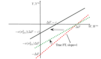
Figure 1: Sketch of the effect of Gaussian uncorrelated noise on symmetry functions, or equivalently on Crooks fluctuation theorem, for a Gaussian work distribution. If $\varepsilon=0$, the measurement noise produces a decrease of the slope of the symmetry function ${Y}^{\text{m}}$ (green dotted line) as compared to $Y$ (red dashed line). This change of slope (a rotation of the line) does not affect the intersection point with the work axis, which corresponds to the free-energy difference, $\Delta F$. When $\varepsilon\neq 0$ however, the symmetry function should be in addition translated by $\varepsilon$ (black solid line). All energies are measured in units of $\beta^{-1}$.

This result can be further simplified using the fluctuation theorem of the true work, namely $\langle e^{-\beta W}\rangle=e^{-\beta\Delta F}$, which is equivalent in this case to $\beta\sigma_{W}^{2}=2(\langle W\rangle-\Delta F)$. Thus, we obtain

$$\Omega({W}^{\text{m}})=\vartheta(\sigma_{\text{SN}}^{2})({W}^{\text{m}}-\Delta F-\sigma_{\text{SN}}^{2}\varepsilon),$$ (37)

in terms of the signal-to-noise ratio and the function $\vartheta(y)=-1/(1+y)$. In this simple case, the Crooks theorem for the distribution of the measured work reads

$${Y}^{\text{m}}({W}^{\text{m}})=\beta\nu(\sigma_{\text{SN}}^{2})({W}^{\text{m}}-\Delta F+\varepsilon),$$ (38)

where ${Y}^{\text{m}}$ is the symmetry function defined in Eq. (9) and $\nu(\sigma_{\text{SN}}^{2})$ is the function:

$$\nu(\sigma_{\text{SN}}^{2})=\frac{\sigma_{\text{SN}}^{2}}{1+\sigma_{\text{SN}}^{2}}=\frac{\sigma_{W}^{2}}{\sigma^{2}+\sigma_{W}^{2}}.$$ (39)

As expected, the Crooks fluctuation theorem is recovered in the absence of noise, i.e. when $\varepsilon=\sigma=0$.

It is apparent with Eq. (38), that the mean of the error shifts the estimation of the free energy by a constant, while the variance of the error affects the slope of the symmetry function. When the mean of the error is zero ($\varepsilon=0)$, only the change of slope occurs. In that case, the Crooks estimator for the free-energy is not biased, while the Jarzynski estimator is. As the amount of noise or coarse-graining increases, the signal to noise ratio decreases, and the slope of the symmetry function decreases. Since the intersection point of this straight line with the work axis remains always equal to the free energy difference, the line undergoes a rotation with respect to the point $W=\Delta F$ on the work axis. When the mean of the error is non-zero, this straight line undergoes in addition an horizontal translation by the amount $\varepsilon$, as shown in Fig 1.

Notice that the change of slope can be equivalently described by a change of temperature. One can thus introduce an effective temperature, equal to the temperature of the heat bath $T$ divided by $\nu(\sigma_{\text{SN}}^{2})$, therefore larger than $T$ since $\nu(\sigma_{\text{SN}}^{2})\leq 1$ according to Eq. (39). In the linear response regime, the same effective temperature will appear in the ratio of the response and correlation functions Verley et al. [2011]. It is important to appreciate however that this notion of effective temperature only applies to situations like the present one where the correction factor in the Crooks relation, namely, $\Omega({W}^{\text{m}})$ is linear. In general, this function is not linear as will become clear in the next examples and in the section reporting numerical results. In such cases, this effective temperature is less meaningful.

To summarize the results of this section, we have shown that an additive correction to the work due to an instrument error or noise leads, in the case that the work and the error are Gaussian distributed, with uncorrelated error, to a multiplicative factor for the temperature, in other words, to an effective temperature. In addition, if the error has nonzero mean, the free-energy estimator is shifted by an amount precisely equal to the mean value of the error.

III.2 Uncorrelated Gaussian error with arbitrary work distribution

We now show how to correct for measurement errors, when the true work distribution is arbitrary, keeping the same assumptions for the error (uncorrelated and Gaussian distributed). We use Eq. (29) in order to relate the probability distribution of the measured work to the probability distribution of the true work. Let us implement a shift by an arbitrary quantity $w$ in the argument of this distribution:

$${P}^{\text{m}}({W}^{\text{m}}-w) =\int dEP({W}^{\text{m}}+E-w)\rho(E),$$ (40)

$${\tilde{P}}^{\text{m}}(-{W}^{\text{m}}-w) =\int dE\tilde{P}(-{W}^{\text{m}}-E-w)\tilde{\rho}(-E)$$

$$=e^{-\beta({W}^{\text{m}}-\Delta F+w)}\times$$

$$\int dEP({W}^{\text{m}}+E+w)\rho(E)e^{-\beta E},$$ (41)

where we have used Eq. (32) in the last step of Eq. (III.2).

After the changes of variables $y={W}^{\text{m}}+E-w$ in (40) and $y={W}^{\text{m}}+E+w$ in (III.2), we get:

$${P}^{\text{m}}({W}^{\text{m}} -w)=\int dyP(y)\rho(y-{W}^{\text{m}}+w),$$ (42)

$${\tilde{P}}^{\text{m}}(-{W}^{\text{m}} -w)=e^{-\beta({W}^{\text{m}}-\Delta F)}\times$$

$$\int dyP(y)\rho(y-{W}^{\text{m}}-w)e^{-\beta(y-{W}^{\text{m}})}$$

$$=e^{-\beta({W}^{\text{m}}-\Delta F)-2w\varepsilon/\sigma^{2}}\times$$

$$\int dyP(y)\rho(y-{W}^{\text{m}}+w)e^{-(\beta-2w/\sigma^{2})(y-{W}^{\text{m}})},$$ (43)

where we have used, in the last step of Eq. (III.2), the explicit form of the error distribution, Eq. (34). It is now clear that choosing $w=\beta\sigma^{2}/2$ leads to:

$$\ln\frac{{P}^{\text{m}}({W}^{\text{m}}-\beta\sigma^{2}/2)}{{\tilde{P}}^{\text{m}}(-{W}^{\text{m}}-\beta\sigma^{2}/2)}=\beta({W}^{\text{m}}-\Delta F+\varepsilon).$$ (44)

Let us first analyze the case of unbiased error, $\varepsilon=0$. We observe that, remarkably, the shift in Eq. (44) removes the bias that was present in the Crooks estimator for measured work and at the same time provides the correct slope for the fluctuation theorem. Thus, the transformation of Eq. (44) solves in a simple way two problems at once: the need to calibrate the experiment against noise and the problem of the bias in the estimator. We shall illustrate this method using simulations in Sec. IV.4.

This result fully agrees with the results of Ref. Ribezzi-Crivellari and Ritort [2014], which is concerned with the inference of free-energies from partial work measurements in the context of single molecule experiments. The authors of this work showed that a shift of the type of Eq. (44) can be used to exploit measurements of the “wrong” work in a symmetric dual trap system, in which one of the traps is fixed, while the other one is moved. Such a transformation allows to recover the correct work distribution when the work distribution is Gaussian and to eliminate the biases in the Jarzynski and Crooks estimators. However, as recognized by the authors, in the case of an asymmetric setup of the traps, a shift of this kind does not permit to recover the correct work distribution (see Ref. Ribezzi-Crivellari and Ritort [2014] for details). This corresponds to our biased case, when $\varepsilon\neq 0$. In such a case, the elimination of the bias in the Crooks estimator is in principle not possible, at least not in the absence of additional information on the error distribution Alemany et al. [2015].

III.3 Correlated Non-Gaussian error distribution

Before moving to more complicated cases where the error is correlated with the true work and is non-Gaussian, let us consider a simple extension of the previous example. Let us assume that the error $E$ is of the form

$$E=\alpha{W}^{\text{m}}+E_{\text{u}},$$ (45)

so that the error is now the sum of a part which is proportional to the measured work, and another part $E_{\text{u}}$, which is still uncorrelated with the true work $W$. By construction, the previous case is recovered for $\alpha=0$. Note that when $W$ is non-Gaussian, this total error will also be non-Gaussian and correlated with $W$.

Let us introduce the probability distribution of the uncorrelated part of the error, $\rho_{u}(E_{\text{u}})$. As before with Eq. (II.2), we consider the joint distribution

$${P}^{\text{m}}({W}^{\text{m}},E_{\text{u}}) ={P}^{\text{m}}({W}^{\text{m}}|E_{\text{u}})\rho_{u}(E_{\text{u}}),$$

$$=P((1+\alpha){W}^{\text{m}}+E_{\text{u}}|E_{\text{u}})\left|\frac{\partial W}{\partial{W}^{\text{m}}}\right|_{E_{\text{u}}}\rho_{u}(E_{\text{u}}),$$

$$=(1+\alpha)P((1+\alpha){W}^{\text{m}}+E_{\text{u}}|E_{\text{u}})\rho_{u}(E_{\text{u}}).$$ (46)

Now, using the property that the variable $E_{\text{u}}$ is uncorrelated with the true work $W$, we obtain

$${P}^{\text{m}}({W}^{\text{m}},E_{\text{u}})=(1+\alpha)P((1+\alpha){W}^{\text{m}}+E_{\text{u}})\rho_{u}(E_{\text{u}}).$$ (47)

An important point is that Eqs. (21) and (24) do not hold in terms of $\rho_{u}(E_{\text{u}})$ and ${P}^{\text{m}}({W}^{\text{m}},E_{\text{u}})$ respectively, since $E_{\text{u}}$ is not the total error, but only its uncorrelated part. For instance, using Eq. (24) and recalling that $E=\alpha{W}^{\text{m}}+E_{\text{u}}$, we will now have:

$$\Omega_{\alpha}({W}^{\text{m}}) =-\frac{1}{\beta}\ln\left<e^{-\beta E}|{W}^{\text{m}}\right>$$

$$=\alpha{W}^{\text{m}}-\frac{1}{\beta}\ln\left<e^{-\beta E_{\text{u}}}|{W}^{\text{m}}\right>$$

$$\equiv\alpha{W}^{\text{m}}+\Omega_{\alpha=0}\big{(}(1+\alpha){W}^{\text{m}}\big{)},$$ (48)

where we have used the subscript $\alpha$ to make explicit the dependence on this parameter, and we have noticed, given that $E_{\text{u}}$ is uncorrelated from $W$, that the second term in the second line of Eq. (III.3) is given exactly by Eq. (31) with the substitution ${W}^{\text{m}}\to(1+\alpha){W}^{\text{m}}$. Note that this result could also be derived by directly computing the joint probability of ${W}^{\text{m}}$ and $E$, which can be easily done as follows:

$${P}^{\text{m}}({W}^{\text{m}},E) =\int dE_{\text{u}}{P}^{\text{m}}({W}^{\text{m}},E_{\text{u}})\delta(E-\alpha{W}^{\text{m}}-E_{\text{u}})$$

$$=(1+\alpha)P({W}^{\text{m}}+E)\rho_{u}(E-\alpha{W}^{\text{m}}),$$ (49)

where we have used Eq. (47) to get the last line. Thus, we have for ${P}^{\text{m}}({W}^{\text{m}})$

$${P}^{\text{m}}({W}^{\text{m}})=(1+\alpha)\int dEP({W}^{\text{m}}+E)\rho_{u}(E-\alpha{W}^{\text{m}}).$$ (50)

Introducing ${P}^{\text{m}}(E|{W}^{\text{m}})={P}^{\text{m}}({W}^{\text{m}},E)/{P}^{\text{m}}({W}^{\text{m}})$, and using directly Eq. (24) together with Eqs. (III.3) and (50), we again obtain (III.3).

Notice that, in particular, when the distributions of the true work and $E_{\text{u}}$ are Gaussian distributed, one obtains

$$\Omega_{\alpha}({W}^{\text{m}}) =\alpha{W}^{\text{m}}+\vartheta(\sigma_{\text{SN}}^{2})\bigg{[}(1+\alpha){W}^{\text{m}}-\Delta F-\sigma_{\text{SN}}^{2}\varepsilon\bigg{]}$$

$$=\alpha\nu(\sigma_{\text{SN}}^{2}){W}^{\text{m}}+\vartheta(\sigma_{\text{SN}}^{2})({W}^{\text{m}}-\Delta F-\sigma_{\text{SN}}^{2}\varepsilon)$$

$$\equiv\alpha\nu(\sigma_{\text{SN}}^{2}){W}^{\text{m}}+\Omega_{\alpha=0}({W}^{\text{m}}).$$ (51)

with $\vartheta$, $\nu$, and $\sigma_{\text{SN}}^{2}$ defined as before, but now in terms of the variance of the uncorrelated part of the error, $\sigma_{u}^{2}$.

It is worth noting, as we see from Eq. (III.3), that this type of correlation only introduces a stretching of the original $\Omega_{\alpha=0}$ via a rescaling of ${W}^{\text{m}}$, plus an additional correction which is linear in ${W}^{\text{m}}$. In particular, in the Gaussian case the stretching can be reabsorbed in the linear correction because $\Omega$ is linear in ${W}^{\text{m}}$ for $\alpha=0$.

For the case of non-Gaussian work distributions but with a Gaussian distribution of $E_{\text{u}}$, it is interesting to seek a relation of the type of Eq. (44) as improved estimators of free energy. Proceeding in the same way as before, the expressions for the forward and reverse probability distributions of the measured work shifted by an amount $w$ are:

$${P}^{\text{m}} ({W}^{\text{m}}-w)=\int dE_{\text{u}}{P}^{\text{m}}({W}^{\text{m}}-w,E_{\text{u}})$$

$$=(1+\alpha)\int dE_{\text{u}}~{}P\big{(}(1+\alpha)({W}^{\text{m}}-w)+E_{\text{u}}\big{)}\rho_{u}(E_{\text{u}}),$$ (52)

and

$${\tilde{P}}^{\text{m}} (-{W}^{\text{m}}-w)=\int dE_{\text{u}}{\tilde{P}}^{\text{m}}(-{W}^{\text{m}},-E_{\text{u}})$$

$$=(1+\alpha)e^{-\beta((1+\alpha)({W}^{\text{m}}+w)-\Delta F)}$$

$$\times\int dE_{\text{u}}~{}P\big{(}(1+\alpha)({W}^{\text{m}}+w)+E_{\text{u}}\big{)}e^{-\beta E_{\text{u}}}\rho_{u}(E_{\text{u}}),$$ (53)

where we have used the relation

$$\rho_{u}(E_{\text{u}})=\tilde{\rho}_{u}(-E_{\text{u}}),$$ (54)

which holds under the same assumptions leading to Eq. (19), as shown in Appendix B.

Let us now assume $\rho_{u}(E_{\text{u}})$ has a mean $\varepsilon$ and a variance $\sigma^{2}_{\text{u}}$, and for any arbitrary $w$, let us introduce the shifted symmetry function

$${Y}^{\text{m}}_{\text{sh}}({W}^{\text{m}},w)=\ln\frac{{P}^{\text{m}}({W}^{\text{m}}-w)}{{\tilde{P}}^{\text{m}}(-{W}^{\text{m}}-w)}.$$ (55)

It can be shown that when $w=w^{*}=\frac{\beta\sigma^{2}_{\text{u}}}{2(1+\alpha)}$, this shifted symmetry function has a simple form:

$${Y}^{\text{m}}_{\text{sh}}({W}^{\text{m}},w^{*})=\beta\bigg{(}(1+\alpha){W}^{\text{m}}-\Delta F+\varepsilon\bigg{)}.$$ (56)

It is important at this point to contrast this result with that obtained in Eq. (44) for $\alpha=0$. Although one obtains again a linear relation for the shifted symmetry function, the slope is not one (in units of $k_{B}T$) but $1+\alpha$. Since a priori neither $\varepsilon$ nor $\sigma^{2}_{\text{u}}$ are known, one should vary the shift parameter $w$ in a plot of ${Y}^{\text{m}}_{\text{sh}}({W}^{\text{m}},w)$ versus ${W}^{\text{m}}$, until the data points collapse on a straight line. From the value of the slope of that line, the value of $\alpha$ can be inferred, and from the actual value of $w^{*}$, the value of $\sigma^{2}_{\text{u}}$ can then be deduced. To apply this method, it is important to be sure that there is a unique value of the optimal shift $w^{*}$. We adress this point in appendix C by proving that indeed there is a unique optimal shift and furthermore that for no other value of $w$, the symmetry function is a linear function of ${W}^{\text{m}}$. Naturally, this proof includes the case $\alpha=0$ considered previously.

When $\varepsilon=0$, this transformation of the symmetry function leads to a complete calibration since no other parameter needs to be fixed, and the correct estimate of the free-energy difference can be recovered, as we shall illustrate numerically in Sec. IV.5. However, when $\varepsilon\neq 0$, the estimator is biased by the mean of the error in a way which can not be fixed in the absence of additional information, as also found in the previous case.

IV Applications to specific choices of dynamics for the measured variable

In this section, we shall apply the theoretical framework developed in previous sections to some specific dynamics for the measured variable. Before we do so, we discuss the choice of measured variables in single molecule experiments (typically position or force). Then, assuming the position is the measured variable, we discuss the consequences of the particular choice of the relation between the dynamics of the measured position and that of the true position. Here, we shall restrict ourselves to two separate cases:

(a) Simple additive noise: the measured position ${x}^{\text{m}}$ and the true position $x$ are related by

$${x}^{\text{m}}(t)=x(t)+\eta(t),$$ (57)

(b) Additive noise with delay: the measured position ${x}^{\text{m}}$ and the true position $x$ are related by

$$\tau_{r}{\dot{x}}^{\text{m}}=x-{x}^{\text{m}}+\eta(t).$$ (58)

From an experimental point of view, case $(a)$ describes purely random measurement errors, which corresponds to the assumption that $\eta$ and $x$ are uncorrelated. In contrast, case $(b)$ describes a case where these variables are correlated because the measurement device introduces a delay between $x(t)$ and its measured value, ${x}^{\text{m}}(t)$. Clearly, both cases are relevant experimentally.

Furthermore, for both dynamics $(a)$ and $(b)$, we assume the distribution of $x(0)$ to be an equilibrium one, while that of ${x}^{\text{m}}(0)$ is not, but corresponds to a stationary non-equilibrium distribution. The system can be prepared in such a state at $t=0$ by starting the evolution at a time $t=-\infty$ in the absence of driving, so that the distributions of $x(0)$ and ${x}^{\text{m}}(0)$ are both stationary. Naturally, both variables $x(0)$ and ${x}^{\text{m}}(0)$ may still be correlated with each other.

IV.1 Choice of measured variable: position vs. force

Before implementing the above dynamics, let us now discuss a practical question regarding the choice of measured variables in single-molecule experiments. In a first setup, where the position is measured, the Hamiltonian which is typically used has the form: $H({x}_{\text{mol}},x;\lambda)=H_{\text{mol}}({x}_{\text{mol}})+H_{\text{coup}}({x}_{\text{mol}},x)+U_{\text{trap}}(x;\lambda)$, where $H_{\text{mol}}({x}_{\text{mol}})$ describes the macromolecule under study (a DNA filament or RNA hairpin, for instance), with ${x}_{\text{mol}}$ labeling the relevant degrees of freedom of that system. This molecule is attached to a bead which is held in an optical trap, and the energy of the bead is given by $U_{\text{trap}}(x;\lambda)$, where $x$ is the position of the bead and $\lambda$ the position of the trap center. Finally, $H_{\text{coup}}({x}_{\text{mol}},x)$ accounts for the coupling between the molecule and the bead.

Usually, the calibration of optical tweezers relies on a harmonic approximation for the trapping potential, $U_{\text{trap}}(x;\lambda)=\kappa(x-\lambda)^{2}/2$, where $\kappa$ denotes the stiffness of the trap and $\lambda$ the position of its center. In this case, the work is

$$W[X] =\int_{0}^{\tau}dt\dot{\lambda}(t)\partial_{\lambda}H\big{(}{x}_{\text{mol}}(t),x(t);\lambda(t)\big{)}$$

$$=\int_{0}^{\tau}dt\dot{\lambda}(t)\partial_{\lambda}U_{\text{trap}}\big{(}x(t);\lambda(t)\big{)}$$

$$=\kappa\int_{0}^{\tau}dt\dot{\lambda}(t)\big{[}\lambda(t)-x(t)\big{]},$$

which does not depend explicitly on the degrees of freedom of the molecule under study characterized by ${X}_{\text{mol}}=\{{x}_{\text{mol}}(t)\}_{t=0}^{\tau}$. In this case, the work on the system is exactly equal to the work on the bead, since the trap is the only term of the Hamiltonian which depends on $\lambda$. The structure of the error in this situation is very simple:

$$E[X,{X}^{\text{m}}]=\kappa\int_{0}^{\tau}dt\dot{\lambda}(t)\big{[}{x}^{\text{m}}(t)-x(t)\big{]},$$ (59)

which shows that the error increases with the driving speed $\dot{\lambda}$ and accumulates with the duration of the experiment $\tau$.

One limitation of such a setup where the position is measured lies in the harmonic approximation used for the trapping potential, an approximation which is expected to fail at large distances from the bead to the center of the trap. Furthermore, recent studies have found great variability in the trap stiffness as a function of the position, even in the region where a constant stiffness was expected Jahnel et al. [2011]. To overcome such issues, a different setup is often preferred, where no assumption on the form of the trapping potential is needed.

In this alternative setup, the force rather than the position, is directed measured from the change in the momentum flux of the light beam impinging on the optical trap Smith et al. [2003]. There is no need to assume a particular form of the trapping potential: one rather measures the force signal, ${f}^{\text{m}}(t)$, which also has some noise (i.e., ${f}^{\text{m}}\neq f$, the true force exerted by the optical trap). The position of the center of the trap is the control parameter which we assume to be error free as we did so far. In some setups one does not have direct access to the position of the trap and one has also to infer it with some error, but we dismiss that possibility here and assume that this is our control parameter . For this setup the work reads:

$$W[\mathcal{F}]=\int_{0}^{\tau}\dot{\lambda}(t)f(t)dt,$$ (60)

with $\mathcal{F}=\{f(t)\}_{t=0}^{\tau}$. Note that the trapping potential $U_{\text{trap}}(x;\lambda)\equiv U_{\text{trap}}(x-\lambda)$, thus, $f=-\partial_{x}U_{\text{trap}}=\partial_{\lambda}U_{\text{trap}}$, and the definition (60) coincides with the Jarzynski work Jarzynski [1997a], *Jarzynski-b, satisfying the nonequilibrium work theorem in the form given by (1). In this case the structure of the error is also very simple

$$W[\mathcal{F}]={W}^{\text{m}}[{\mathcal{F}}^{\text{m}}]-\int_{0}^{\tau}dt\dot{\lambda}(t)\big{[}{f}^{\text{m}}(t)-f(t)\big{]}.$$ (61)

It is worth noting that both, Eq. (59) and Eq. (61), have the same structure. In addition, note that the assumption that $\lambda$ is error free is not very dangerous. This can be seen as follows. In the first setup, one can redefine the distances and consider the error in measuring $\lambda-x$ instead of $x$ alone. In the second case, one does not need to know the value of $\lambda$ in order to calculate the work because the force is directly recorded. In both cases what remains free is the pulling velocity, $\dot{\lambda}$, which is very well controlled even if $\lambda$ itself is not.

Since it is a rather simple matter to switch between notations for the force setup and that for the position setup, we limit ourselves in the rest of the paper to only one case, which we chose to be the position setup.

IV.2 Corrected Jarzynski estimator

Let us derive the correction to the Jarzynski estimator in the presence of measurement error $\eta$ within dynamics $(a)$ defined in Eq. (57).

$$\langle e^{-\beta{W}^{\text{m}}}\rangle_{\Lambda}= \int\mathcal{D}{X}^{\text{m}}{\mathcal{P}}^{\text{m}}[{X}^{\text{m}}]e^{-\beta{W}^{\text{m}}[{X}^{\text{m}}]}$$

$$= \int\mathcal{D}{X}^{\text{m}}\mathcal{D}X{\mathcal{P}}_{\text{e}}[{X}^{\text{m}}|X]\mathcal{P}[X]e^{-\beta{W}^{\text{m}}[{X}^{\text{m}}]}$$

$$= \int\mathcal{D}X\mathcal{P}[X]e^{-\beta W[X]}\big{\langle}e^{\beta E[{X}^{\text{m}},X]}\big{|}X\big{\rangle}_{\Lambda}.$$ (62)

In this case one has ${\mathcal{P}}_{\text{e}}[{X}^{\text{m}}|X]=\mathcal{P}[\boldsymbol{\eta}|X]\equiv\mathcal{P}_{\eta}[\boldsymbol{\eta}]$, where $\mathcal{P}_{\eta}$ is the path probability density of the error trajectory $\boldsymbol{\eta}=\{\eta(t)\}_{0}^{\tau}$. Thus, since the error in Eq. (59) is a linear functional of $\boldsymbol{\eta}$, it can be integrated explicitly. We thus have

$$\langle e^{-\beta{W}^{\text{m}}}\rangle_{\Lambda} =\big{\langle}e^{-\beta W[X]}\big{\rangle}_{\Lambda}e^{K_{\eta}[\kappa\beta\dot{\lambda}]}$$

$$\equiv e^{-\beta(\Delta F-(1/\beta)K_{\eta}[\kappa\beta\dot{\lambda}])},$$ (63)

where we have used the Jarzynski equality, Eq. (1), and we have introduced the generating functional of the cumulants of $\mathcal{P}_{\eta}$, $K_{\eta}[J]=\ln\int\mathcal{D}\boldsymbol{\eta}\mathcal{P}_{\eta}[\boldsymbol{\eta}]\exp[\int dtJ(t)\eta(t)]$. From this, we obtain the following estimate of the free energy, $\Delta\hat{F}(N)$ as:

$$\Delta\hat{F}(N)=\Delta F-\frac{1}{\beta}K_{\eta}[\kappa\beta\dot{\lambda}].$$ (64)

As stated before, the bias in the estimation of the free-energy difference only depends on the statistical properties of the error associated to measurement apparatus. This result is fully compatible with the expression of the correction $R=k_{B}TK_{\eta}[\kappa\beta\dot{\lambda}]$ obtained from Eq. (21) when $\rho(E)$ is assumed to be symmetric under time-reversal symmetry.

Let us discuss now the validity of the factorization property Eq. (28), or equivalently, of the convolution formula of Eq. (29). To illustrate this, let us consider a simple case where the optical trapping is assumed to be parabolic, whereas in reality, it is not. In that case, the measured work is

$${W}^{\text{m}} ={\kappa}^{\text{m}}\int_{0}^{\tau}dt\dot{\lambda}(t)[\lambda(t)-{x}^{\text{m}}(t)]$$

$$={\kappa}^{\text{m}}\int_{0}^{\tau}dt\dot{\lambda}(t)[\lambda(t)-x(t)-\eta(t)]$$ (65)

while the true work reads

$$W=\int_{0}^{\tau}dt\dot{\lambda}(t)\partial_{\lambda}U_{\text{trap}}(\lambda-x),$$ (66)

where we have introduced the experimental stiffness of the trap, ${\kappa}^{\text{m}}$, and the dynamics of Eq. (57) with $\eta(t)$ uncorrelated with $x(t)$. Indeed, the error at time $\tau$, $E=W-{W}^{\text{m}}$, is in general correlated with the values of $W$ not only at time $\tau$, but even at earlier times. This is very easy to see by noting, from Eq. (IV.2), that we have $\lambda(t)-x(t)={\dot{W}}^{\text{m}}(t)/{\kappa}^{\text{m}}\dot{\lambda}(t)+\eta(t)\equiv({\kappa}^{\text{m}}\dot{\lambda}(t))^{-1}[\dot{W}(t)-\dot{E}(t)]+\eta(t)$. Substituting this back in (66) we clearly see that $W$ and $E$ are in general correlated in a highly non-local way in time even in this simple case, so that Eqs. (28) and (29) do not hold anymore.

It is worth noting, however, that there is a particular case where one can still make the assumption that correlations are local in time. This happens when the true trapping potential is still parabolic, but the stiffness is not correctly estimated, its value is $\kappa\neq{\kappa}^{\text{m}}$. It is easy to see that in this case we have

$$W =\kappa\int_{0}^{\tau}dt\dot{\lambda}(t)[\lambda(t)-x(t)]$$

$$=\kappa\int_{0}^{\tau}dt\dot{\lambda}(t)[\lambda(t)-{x}^{\text{m}}(t)+\eta(t)]$$

$$=\frac{\kappa}{{\kappa}^{\text{m}}}{\kappa}^{\text{m}}\int_{0}^{\tau}dt\dot{\lambda}(t)[\lambda(t)-{x}^{\text{m}}(t)]+\kappa\int_{0}^{\tau}dt\dot{\lambda}(t)\eta(t)$$

$$\equiv\frac{\kappa}{{\kappa}^{\text{m}}}{W}^{\text{m}}+E_{\text{u}},$$ (67)

where $E_{\text{u}}=\kappa\int_{0}^{\tau}dt\dot{\lambda}(t)\eta(t)$ is still uncorrelated from $W$, while the error $E=W-{W}^{\text{m}}=[(\kappa/{\kappa}^{\text{m}})-1]{W}^{\text{m}}+E_{\text{u}}$ is not. This shows that miscalibration of the trap stiffness introduces a correlated error of the form considered before in Eq. (45), with $\alpha$ given by $\alpha=\kappa/{\kappa}^{\text{m}}-1$.

IV.3 Fraction of second-law violating trajectories in terms of measured work

Clearly, the fraction of trajectories that transiently violate the second law is different for the true and the measured works. For Gaussian distributed work, this fraction is analytically calculable, following the method of Sahoo et al. [2011]. We begin with the relation

$$\int d{W}^{\text{m}}P({W}^{\text{m}})e^{-\beta{W}^{\text{m}}}=e^{-\beta(\Delta F-R)}$$

$$=\frac{1}{\sqrt{2\pi\sigma_{{W}^{\text{m}}}^{2}}}\int d{W}^{\text{m}}\exp\bigg{[}-\frac{({W}^{\text{m}}-\left<{W}^{\text{m}}\right>)^{2}}{2\sigma_{{W}^{\text{m}}}^{2}}-\beta{W}^{\text{m}}\bigg{]}.$$ (68)

A simplification of this relation leads to

$$\frac{1}{2}\beta\sigma_{{W}^{\text{m}}}^{2}=\left<{W}^{\text{m}}\right>-\Delta F+R,$$ (69)

where $R$ is given by Eq. (35). Now we can readily calculate the fraction of atypical trajectories (i.e. the ones that transiently violate the second law) by integrating the work probability distribution from $-\infty$ to $\Delta F$:

$${\mathfrak{f}}^{\text{m}} =\frac{1}{\sqrt{2\pi\sigma_{{W}^{\text{m}}}^{2}}}\int_{-\infty}^{\Delta F}d{W}^{\text{m}}\exp\bigg{[}-\frac{({W}^{\text{m}}-\left<{W}^{\text{m}}\right>)^{2}}{2\sigma_{{W}^{\text{m}}}^{2}}\bigg{]}$$

$$=\frac{1}{2}\text{erfc}\bigg{[}\frac{\left<{W}^{\text{m}}\right>-\Delta F}{\sqrt{2\sigma_{{W}^{\text{m}}}^{2}}}\bigg{]}.$$ (70)

Let us assume that the error in the measured work has non-zero mean $\varepsilon$. Using the definition of measured work and the fluctuation theorem for true work, we have:

$$\left<W\right> =\left<{W}^{\text{m}}\right>+\varepsilon=\Delta F+\frac{1}{2}\beta\sigma_{W}^{2}.$$ (71)

Using (69), one then obtains

$${\mathfrak{f}}^{\text{m}} =\frac{1}{2}\text{erfc}\bigg{[}\frac{1}{2}\frac{\left<{W}^{\text{m}}\right>-\Delta F}{\sqrt{\beta^{-1}(\left<{W}^{\text{m}}\right>-\Delta F+R)}}\bigg{]}$$

$$=\frac{1}{2}\text{erfc}\left[\frac{1}{2}\frac{\frac{1}{2}\beta\sigma_{W}^{2}-\varepsilon}{\sqrt{\frac{1}{2}(\sigma_{W}^{2}+\sigma^{2})}}\right].$$ (72)

We note that

$${\mathfrak{f}}^{\text{m}} =\frac{1}{2}\text{erfc}\bigg{[}\frac{\beta}{2\sqrt{2}}~{}\frac{\sigma_{W}^{2}-2\beta^{-1}\varepsilon}{\sqrt{\sigma_{W}^{2}+\sigma^{2}}}\bigg{]}\geq\frac{1}{2}\text{erfc}\bigg{[}\frac{\beta}{2}\sqrt{\frac{\sigma_{W}^{2}}{2}}\bigg{]}=\mathfrak{f},$$ (73)

if $\varepsilon\geq 0$. In that case, measurement errors cause an overestimation of the fraction of trajectories transiently violating the second law. Furthermore, note that ${\mathfrak{f}}^{\text{m}}>1/2$ only if the argument of the error function is negative. Thus, we will observe apparent violations of the second law if the error is positive and sufficient large so that $\varepsilon>\beta\sigma_{W}^{2}/2$. In this case, the mean of the measured work is less than $\Delta F$.

It is instructive to illustrate this result with a simple example. Consider a Brownian particle following the Langevin Equation

$$\dot{x}=-\kappa(x-\lambda)+\xi(t),$$ (74)

where $\xi(t)$ is the Gaussian random white noise: $\left<\xi(t)\right>=0$, and $\left<\xi(t)\xi(s)\right>=2T\delta(t-s)$. The system is initially at equilibrium with a heat bath at temperature $T$, and is thereafter perturbed by a time-dependent linear protocol $\lambda(t)=at/\tau\equiv bt$, where $b=a/\tau$. The average work done on the particle is given by

$$\left<W\right> =\int_{0}^{\tau}\dot{\lambda}(\lambda-\left<x\right>)dt$$

$$=b\int_{0}^{\tau}(bt-\left<x\right>)dt.$$ (75)

Using Eqs. (74) and (75), we arrive at

$$\left<W\right> =\frac{b^{2}}{\kappa}\bigg{[}\tau-\frac{1-e^{-\kappa\tau}}{\kappa}\bigg{]}.$$ (76)

With the present form of trapping potential, it is simple to check that the partition function is independent of $\lambda$ and as a result $\Delta F=0$. Thus, to allow ${\mathfrak{f}}^{\text{m}}$ to be greater than 1/2, one should have $\left<{W}^{\text{m}}\right><0$, or equivalently $\varepsilon>\left<W\right>$, which means:

$$\varepsilon>\frac{b^{2}}{\kappa}\bigg{[}\tau-\frac{1-e^{-\kappa\tau}}{\kappa}\bigg{]}.$$ (77)

Using the inequality $e^{r}\geq 1+r$, it can be easily checked that the right hand side is always non-negative. If the measured position ${x}^{\text{m}}$ and the true position $x$ are related by Eq. (57) assuming $\eta$ is another Gaussian distributed white noise, then the mean of $\eta$ is related to $\varepsilon$ as

$$\left<\eta\right> =\frac{\varepsilon}{b\tau}.$$ (78)

Then the condition (77) translates to

$$\left<\eta\right>>\frac{b}{\kappa}\bigg{[}1-\frac{1-e^{-\kappa\tau}}{\kappa\tau}\bigg{]}.$$ (79)

For large enough value of $\tau$, we then have the condition $\left<\eta\right>>b/\kappa$. When this condition is satisfied, we expect the mean of the Gaussian distribution of ${W}^{\text{m}}$ to lie to the left of the ${W}^{\text{m}}=0$ axis. This is shown in figure 2, where the distributions for the true work and the measured work have been plotted, with $b=0.5$, $\kappa=1$ and $\left<\eta\right>=1$. Clearly, the mean of the distribution for ${W}^{\text{m}}$ lies to the left of the ${W}^{\text{m}}=0$ axis, unlike for the distribution of the true work.

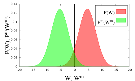
Figure 2: Plots of measured and true work distributions (work being measured in unit of $k_{B}T$), when $\tau=20$ and $\left<\eta\right>>b/\kappa$. The parameters used are $b=0.5$, $\kappa=1$ and $\left<\eta\right>=1$.

This example shows that a sufficiently large and positive mean error drastically alters our estimation of the fraction of trajectories that violate the second law. Naturally, nothing of that sort would occur if $\varepsilon<0$. Below, we test the main results of the paper regarding modified fluctuation theorems obtained in previous sections numerically. We start with the case of uncorrelated Gaussian error and then we consider an example of correlated non-Gaussian error.

IV.4 Numerics for the case of uncorrelated Gaussian errors

We begin by verifying the relation (44), for a system that is subjected to the time-dependent potential

$$V(x,t)=\frac{1}{2}\kappa(x-\lambda(t))^{2}-\frac{1}{2}x^{2}+\frac{1}{4}x^{4},$$ (80)

where the first term on the RHS represents the force acting on the system due to the harmonic trap, the center of which is positioned at $\lambda(t)$, and $\kappa$ is the stiffness constant of the trap. The second and third terms represent a double-well potential that the particle sees in addition to the trap potential. The system follows the overdamped Langevin equation of motion:

$$\dot{x}=-\partial_{x}V(x,t)+\xi(t),$$ (81)

$\xi(t)$ being the Gaussian thermal white noise with zero mean: $\left<\xi(t)\right>=0$, $\left<\xi(t)\xi(t^{\prime})\right>=2T\delta(t-t^{\prime})$.

We have chosen the parameter $\lambda(t)$ to be $A\sin\omega t$, which is a simple sinusoidal drive of amplitude $A$ and frequency $\omega$. The protocol is applied for a time $\tau=\pi/2\omega$, which is one-fourth of the drive period. The error in the measurement corresponds to case $(a)$, with the additional assumption that $\eta$ is a Gaussian white noise of mean zero and of autocorrelation function $\left<\eta(t)\eta(t^{\prime})\right>=\sigma_{\eta}^{2}\delta(t-t^{\prime})$. The error in the measurement of the work is also Gaussian, since it is linear in $\eta$:

$$E=\int_{0}^{\tau}dt\dot{\lambda}(t)\eta(t).$$ (82)

We can then derive the variance of the error to be

$$\sigma^{2} =\sigma_{\eta}^{2}\int_{0}^{\tau}dt\int_{0}^{\tau}dt^{\prime}\delta(t-t^{\prime})\dot{\lambda}(t)\dot{\lambda}(t^{\prime})$$

$$=\sigma_{\eta}^{2}A^{2}\omega^{2}\int_{0}^{\tau}dt\cos^{2}\omega t$$

$$=\sigma_{\eta}^{2}A^{2}\omega\pi/4$$ (83)

for $\tau=\pi/2\omega$. With the choice of parameters $\sigma_{\eta}^{2}=0.5$, $A=2$, and $\omega=1$, we obtain $\sigma^{2}\simeq 1.571$. The required shift in ${W}^{\text{m}}$ is $R=\beta\sigma^{2}/2\simeq 0.785$.

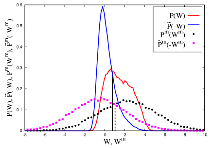
Figure 3: The distributions $P(W)$, $\tilde{P}(-W)$, ${P}^{\text{m}}(W)$ and ${\tilde{P}}^{\text{m}}(-W)$ for the above potential. They are clearly non-Gaussian. The intersection point of $P(W)$ and $\tilde{P}(-W)$ gives the value of $\Delta F\simeq 0.82$. The solid vertical line shows the value of $W$ at the intersection of $P(W)$ and $\tilde{P}(-W)$, whereas the dotted vertical line shows the value of ${W}^{\text{m}}$ at the intersection of ${P}^{\text{m}}(W)$ and ${\tilde{P}}^{\text{m}}(-W)$. We have chosen $\sigma_{\eta}^{2}=2$, $A=2$, $k_{B}T=1$, $\kappa=1$, $\gamma=1$ and $\sigma_{\eta}^{2}=2$.

Figure 3 shows the distributions of the true and the measured works for the above potential, for forward and reverse drivings. The parameters chosen have been mentioned in the figure caption. The non-Gaussian nature of these distributions is apparent, as is the bias in the determination of free energy from Crooks relation. Indeed, the crossing point of $P(W)$ and $\tilde{P}(-W)$ (which gives the free energy change $\Delta F\simeq 0.82$) is clearly different from that of the distributions $P({W}^{\text{m}})$ and $\tilde{P}(-{W}^{\text{m}})$. We also note that the variance of measured work in either the forward or the reverse process is higher than that of the true work.

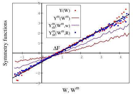
Figure 4: Symmetry functions for the true work $Y(W)$ (red filled circles), for measured work ${Y}^{\text{m}}({W}^{\text{m}})$ (brown solid line) and shifted symmetry functions of measured works ${Y}^{\text{m}}_{\text{sh}}({W}^{\text{m}},w)$ with intermediate (dashed line) and optimal (blue filled squares) values of the shift $w$, as defined in Eqs. (8), (9) and (55) respectively. All energies are measured in units of $\beta^{-1}$. The black solid line is a linear fit for $Y(W)$. We have chosen $\sigma_{\eta}^{2}=0.5$, all other parameters being the same as in figure 3. The free energy, obtained from the Jarzynski equality is $\Delta F\simeq 0.82$.

In figure 4, we show the symmetry functions for the true and the measured works, as a function of $W$, which are denoted by $Y(W)$ and ${Y}^{\text{m}}({W}^{\text{m}})$, respectively. The black solid line is the linear fit for $Y(W)$, which as expected corresponds to a straight line of slope one. In contrast, the symmetry function ${Y}^{\text{m}}({W}^{\text{m}})$ for the measured work is not a linear function as expected theoretically.

In view of the exact relations derived for shifted symmetry functions in Eqs. (42)-(44), we consider again shifted symmetry functions defined as in Eq. (55). Initially the appropriate value of $w$ is unknown, but it is possible to tune this parameter so as to find the point where $w=R$. Here, since $\varepsilon=0$, the correct value is $R=\beta\sigma^{2}/2\simeq 0.785$, at which point according to Eq. (44), the shifted symmetry function has a simpler form, namely:

$${Y}^{\text{m}}_{\text{sh}}({W}^{\text{m}},R)=\beta({W}^{\text{m}}-\Delta F).$$ (84)

In fig. 4, these shifted symmetry functions are shown for intermediate values of $w$ and for the most appropriate value $w=R$, which makes the data points collapse on the black line of slope 1. This shows that at least in this case where $\varepsilon=0$, it is indeed possible to tune the value of $w$ to infer the correct value of the free energy difference using only the noisy data of measured works. The correct value of the free energy in this simulation is $\Delta F\approx 0.82$, which corresponds well to the point where the symmetry function of the true work and the shifted symmetry function of the measured work intersect the $W$-axis. In case we had $\varepsilon\neq 0$, we would be able to collapse the data on a straight line but would not be able to infer the correct $\Delta F$.

IV.5 Numerics for the case of correlated non-Gaussian error

We now verify numerically our results obtained for non-Gaussian correlated error of the type $E=E_{\text{u}}+\alpha{W}^{\text{m}}$. This kind of error can arise in two situations: First, when there is a miscalibration of the trap stiffness used for the evaluation of the measured work, as discussed in subsection IV.2. Secondly, when the relation between the measured position and the true position is modified with respect to the one given by Eq. (57). It can be shown that the correct modification compatible with an error of the form $E=E_{\text{u}}+\alpha{W}^{\text{m}}$ is:

$${x}^{\text{m}}=\frac{x+\alpha\lambda(t)+\eta}{1+\alpha},$$ (85)

where as before $\lambda$ denotes the position of the trap, while $\eta$ represents a random process which is uncorrelated from $x(t)$.

In our numerical simulations, we have implemented the second case for convenience. In figure 5, we have plotted the symmetry functions for the true and the measured works (filled circles and solid line in brown, respectively). Our parameters are the same as in figure 4. As in the case of figure 4, the symmetry function for ${W}^{\text{m}}$ is not a linear function of ${W}^{\text{m}}$.

Improved free energy estimators can be constructed using shifted symmetry functions defined in Eq. (55) and by tuning the shift parameter $w$ until the data points collapse on a straight line. According to Eq. (56), the slope of the straight line at the collapse can be used to determine $\alpha$, while the optimal value of $w$ provides information on $\sigma^{2}_{\text{u}}$ the variance of $E_{\text{u}}$, since they are related by $w^{*}=\beta\sigma^{2}_{\text{u}}/(2(1+\alpha))$. From the linear fit of the data points for the optimal shift, we obtain a slope of $1.82$, which gives $\alpha=0.82$, in agreement with the actual value of 0.8. In the inset of figure 5, we show the plot for the $\chi^{2}$ values for this linear fit with the minimum of the plot coinciding with the optimal value $w^{*}\simeq 0.44$. This confirms that this method can be used practically for determining $\alpha$ and $\sigma^{2}_{\text{u}}$.

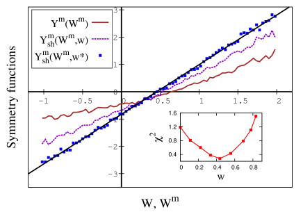
Figure 5: Symmetry functions for ${W}^{\text{m}}$ without shift (brown solid line), intermediate shift $w=0.22$ (violet dashed line) and optimal shift $w^{*}=0.44$ (blue filled squares). The black solid line is the linear fit for the data points for optimal shift. The slope of this line is 1.82, which is very close to the actual value 1.8. The inset shows a plot of the $\chi^{2}$ of a linear fit of ${Y}^{\text{m}}({W}^{\text{m}},w)$ for various values of $w$. The minimum is reached at the optimal value $w=w^{*}$. Parameters: same as in figure 4.

IV.6 Correlated error due to finite delay in measurements

We next turn our attention to symmetry functions for measured work, when the measurement outcome is obtained after a time delay as described by case $(b)$ in Eq. (58). We rewrite the equations for $x$ and ${x}^{\text{m}}$ below:

$$\gamma\dot{x} =\kappa(\lambda(t)-x)+\xi(t);$$

$$\tau_{r}{\dot{x}}^{\text{m}} =x-{x}^{\text{m}}+\eta(t).$$ (86)

Both, $\xi(t)$ and $\eta(t)$ are Gaussian white noises, of mean zero and of autocorrelation function $\left<\xi(t)\xi(t^{\prime})\right>=2\gamma T\delta(t-t^{\prime})$ and $\left<\eta(t)\eta(t^{\prime})\right>=\sigma_{\eta}^{2}\delta(t-t^{\prime})$. We let the system evolve under these two equations in the absence of driving, $\lambda=0$, for a time much larger than $\gamma/\kappa$ as well as $\tau_{r}$, so that the true position variable $x$ is at equilibrium at time $t=0$, while the measured position ${x}^{\text{m}}$ is in a non-equilibrium steady state.

Due to the delay, the state variable ${x}^{\text{m}}$ obeys a non-markovian dynamics, and as a result, the error is correlated with the true work in a complex way. Linear Langevin systems with time delays have been studied extensively in the literature on feedback systems Munakata and Rosinberg [2014], Horowitz and Sandberg [2014]. In that respect, our problem is simpler in that there is no feedback since the first equation in Eq. (86) does not contain the variable ${x}^{\text{m}}$. Yet, the correlations between the error $E$ and the true work are more complex than that considered in Eq. (45) in terms of the parameter $\alpha$. In particular, the error does not transform under time reversal as $\rho(E)=\tilde{\rho}(-E)$ because the quantity ${S}_{\text{e}}$ which has been assumed to vanish in section II does not vanish here.

Fortunately, due to the linearity of the equations, the true and the measured works are also Gaussian distributed, being linear in $x$ and ${x}^{\text{m}}$, respectively. Thus, we only need to focus on the mean and the variance of the measured work without having to consider the statistics of the error. The mean and the variance of the measured work can be obtained by direct integration of Eq. (86) after some algebra, which is detailed in the appendix D. From the formal expressions, one notices that the mean $\left<{W}^{\text{m}}\right>$ as well as the variance $\sigma_{{W}^{\text{m}}}^{2}$ are even under time-reversal symmetry, which implies $P({W}^{\text{m}})=\tilde{P}({W}^{\text{m}})$. Using the fact that the distributions are Gaussian, one then arrives at the relation

$${Y}^{\text{m}}({W}^{\text{m}}) \equiv\ln\frac{P({W}^{\text{m}})}{\tilde{P}(-{W}^{\text{m}})}=\frac{2{W}^{\text{m}}\left<{W}^{\text{m}}\right>}{\sigma_{{W}^{\text{m}}}^{2}}.$$ (87)

The slope of the symmetry function is therefore:

$$\beta_{eff}=\frac{2\left<{W}^{\text{m}}\right>}{\sigma_{{W}^{\text{m}}}^{2}}.$$ (88)

It can be interpreted as an inverse effective temperature in view of the Crooks relation ${Y}^{\text{m}}({W}^{\text{m}})=\beta_{eff}{W}^{\text{m}}$, which takes this form since the free energy difference is zero in the present setup.

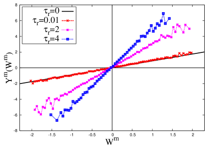
Figure 6: Symmetry functions ${Y}^{\text{m}}({W}^{\text{m}})$ for various values of the relaxation time $\tau_{r}$. The solid line is of slope $\sigma_{W}^{2}/(\sigma^{2}_{\text{u}}+\sigma_{W}^{2})=0.878$, as expected when the error becomes uncorrelated with the work. The other parameters are: $a=1$, $k_{B}T=1$, $\sigma_{\eta}^{2}=0.1$ and $\tau=1$.

The symmetry functions for different values of $\tau_{r}$ for the applied linear protocol $\lambda(t)=at/\tau$ have been plotted in figure 6. As expected all these curves are straight lines going through the origin, which confirms the interpretation in terms of effective temperatures. Note that this effective temperature depends on both $\tau_{r}$ and $\tau$ as we discuss now.

As $\tau_{r}$ is increased, the inverse effective temperature increases, i.e. the effective temperature decreases. This is expected since by increasing $\tau_{r}$, the fluctuations of ${x}^{\text{m}}$ become more and more smooth as a result of filtering the fluctuations of the true position for longer measurement times. This filtering translates into a decrease of the fluctuations of the measured position, i.e. a decrease of their effective temperature. For $\tau_{r}\to 0$ (red curve), we recover the effective temperature, which has been obtained in Eq. (39) for the case of dynamics (a). That effective temperature is necessarily larger than the bath temperature and is shown by the black solid line.

From the point of view of the measured position, the true position appears as a perturbation, or as a driving force which is imposed from the outside. This driving force imposes a new time scale $\gamma/\kappa$ on the dynamics of the measured position, which would evolve otherwise with the time scale $\tau_{r}$. According to Ref. Dieterich et al. [2015], the regime for which an effective temperature is expected is the one for which $\tau_{r}\geq\gamma/\kappa$, which corresponds to the case where we find a small effective temperature. Interestingly, we also have a well-defined effective temperature in the other regime $\tau_{r}\leq\gamma/\kappa$, which we have analyzed before.

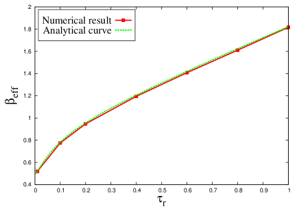
Figure 7: Inverse effective temperature $\beta_{eff}$ as a function of the relaxation time $\tau_{r}$. The parameters are $a=1$, $\tau=0.1$, $\sigma_{\eta}^{2}=0.1$, $k_{B}T=\kappa=\gamma=1$. The green dotted line is an exact evaluation using Eq. (88) and appendix D, while the red solid line is the simulation curve.

Naturally our case differs from that of Ref. Dieterich et al. [2015], which is concerned with steady states, while we do not. This can also be seen from the dependence of our results on the time scale associated with the duration of the driving $\tau$. In figure 7, we show the variation of the slope of ${Y}^{\text{m}}({W}^{\text{m}})$, namely $\beta_{eff}$, as a function of $\tau_{r}$, when $\tau=0.1$. The other parameters are as mentioned in the figure caption. We find a very good agreement with the simulations in the full range of variation of $\tau_{r}$. The same plots for higher observation time, $\tau=1$, is shown in figure 8. Once again, there is a good agreement with the numerics, which in this case is a straight line of slope $\approx 0.95$.

In the limit $\tau_{r}\to\infty$, one can show from the exact expression of the slope of ${Y}^{\text{m}}$ provided in appendix D that it behaves as $2\kappa\tau_{r}/(2\gamma T+\sigma_{\eta}^{2}\kappa^{2})$, which correctly predicts the slope of the straight line in figure 8.

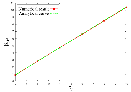
Figure 8: Same plot as above, with $\tau=1$, other parameters being the same.

V Relation to information theory and feedback

V.1 Equilibrium initial conditions

The corrections $\Omega$ and $R$ are factors modifying the fluctuation theorems in the presence of coarse-graining or noise. As shown below, similar factors have been introduced before in the context of Fluctuation theorems with feedback Shiraishi and Sagawa [2015], Sagawa and Ueda [2010] and on related second-law like inequalities with information Horowitz and Sandberg [2014], Munakata and Rosinberg [2014].

Let us consider the probability for a true trajectory in phase space, $\mathcal{P}[X]$, and the one for the measured trajectory ${\mathcal{P}}^{\text{m}}[{X}^{\text{m}}]$. These two probabilities are related by

$${\mathcal{P}}^{\text{m}}[{X}^{\text{m}}]=\int\mathcal{D}X{\mathcal{P}}_{\text{e}}[{X}^{\text{m}}|X]\mathcal{P}[X],$$ (89)

where the difference between both distributions is contained in ${\mathcal{P}}_{\text{e}}$. In particular, when the measurement process is free of error, ${\mathcal{P}}_{\text{e}}[{X}^{\text{m}}|X]=~{}\delta[{X}^{\text{m}}-X]$, then ${\mathcal{P}}^{\text{m}}[{X}^{\text{m}}]=\mathcal{P}[{X}^{\text{m}}]$.

In the experiment, only the coarse-grained trajectory ${X}^{\text{m}}$ is available. The amount of information provided by ${X}^{\text{m}}$ about the true trajectory $X$ is quantified by the mutual information

$$I_{x}=\int\mathcal{D}X\mathcal{D}{X}^{\text{m}}\mathcal{P}[{X}^{\text{m}},X]\ln\frac{\mathcal{P}[{X}^{\text{m}},X]}{\mathcal{P}[X]{\mathcal{P}}^{\text{m}}[{X}^{\text{m}}]},$$ (90)

where $\mathcal{P}[{X}^{\text{m}},X]$ is the joint path probability of true and measured trajectories. In particular, if ${X}^{\text{m}}$ and $X$ are independent random variables, $I_{x}=0$, implying that no information can be extracted on $X$ from the knowledge of ${X}^{\text{m}}$. Introducing the stochastic mutual information, $\mathcal{I}_{x}[{X}^{\text{m}},X]$, through the relation

$$\frac{{\mathcal{P}}^{\text{m}}[{X}^{\text{m}}]}{{\mathcal{P}}_{\text{e}}[{X}^{\text{m}}|X]}=e^{-\mathcal{I}_{x}[{X}^{\text{m}},X]},$$ (91)

we can write the mutual information simply as $I_{x}=~{}\langle\mathcal{I}_{x}[{X}^{\text{m}},X]\rangle\geq 0$. Then, combining Eqs. (91) and (10), we may write

$${\mathcal{P}}^{\text{m}}[{X}^{\text{m}}]\tilde{\mathcal{P}}[\tilde{X}]=\mathcal{P}[{X}^{\text{m}},X]e^{-\beta(W[X]-\Delta F)-\mathcal{I}_{x}[{X}^{\text{m}},X]}.$$ (92)

It is worth noting that, in terms of the true work, a Jarzynski relation as for feedback processes Sagawa and Ueda [2010] follows immediately:

$$\big{\langle}e^{-\beta(W[X]-\Delta F)-\mathcal{I}_{x}[{X}^{\text{m}},X]}\big{\rangle}_{\Lambda}=1.$$ (93)

Since the Jarzynski relation holds in terms of $W[X]$, the second law derived from Eq. (93), $\beta(\langle W\rangle-\Delta F)\geq-I_{x}$ is uninformative, since $I_{x}\geq 0$ while $\beta(\langle W\rangle-\Delta F)\geq 0$ holds in this case. We shall thus turn instead towards a modified Jarzynski relation in terms of the measured work, which is experimentally accessible.

A key point is to recognize that the lack of knowledge on the system is represented by two contributions. One is, of course, the error in the measurement of the true trajectory. The second is, as stated above, the mutual information which quantifies, how much one can infer about the true trajectories from the measured ones. We can thus introduce a unified quantity measuring both effects as

$$\Delta_{x}[{X}^{\text{m}},X]=\beta E[{X}^{\text{m}},X]+\mathcal{I}_{x}[{X}^{\text{m}},X].$$ (94)

With this, and using Eq. (5), Eq. (92) can be rewritten as

$${\mathcal{P}}^{\text{m}}[{X}^{\text{m}}]\tilde{\mathcal{P}}[\tilde{X}]=\mathcal{P}[{X}^{\text{m}},X]e^{-\beta({W}^{\text{m}}[{X}^{\text{m}}]-\Delta F)-\Delta_{x}[{X}^{\text{m}},X]}.$$ (95)

We thus have after direct integration

$$\big{\langle}e^{-\beta({W}^{\text{m}}[{X}^{\text{m}}]-\Delta F)-\Delta_{x}[{X}^{\text{m}},X]}\big{\rangle}_{\Lambda}=1.$$ (96)

Comparing the Jarzynski relation for feedback processes Sagawa and Ueda [2010] with Eq. (96), we see that there is a similar structure, despite the fact that there is no feedback in our case. An important difference between both cases is that $\langle\Delta_{x}\rangle$ does not have a definite sign, because there is no particular sign for the measurement error. However, if the distribution of the measurement errors has non-negative mean, then $\langle\Delta_{x}\rangle$ is non-negative, since $I_{x}\geq 0$. It is also interesting to note, by simple inspection of Eq. (6), that $\exp(\beta R)$ is the analog of the efficacy parameter introduced in Sagawa and Ueda [2010] for feedback processes and denoted $\gamma$ in that reference.

V.2 Generalization to the case of nonequilibrium initial distribution

In this sub-section only, we extend the results of previous sections to situations where the initial distribution of the true variable $x(0)$ is not an equilibrium one, but rather an arbitrary distribution. To emphasize this difference, let us now denote the corresponding full trajectory with a prime as $X^{\prime}=\{x(t)\}_{t=0}^{\tau}$, to distinguish it from the trajectory which we had denoted $X$ so far. When the initial condition $x(0)$ is not an equilibrium one, the modified Crooks relation becomes Esposito and van den Broeck [2011], Lahiri and Jayannavar [2015]

$$\frac{\tilde{P}[\tilde{X}^{\prime}]}{P[X^{\prime}]} =e^{-\beta(W-\Delta F)+\Delta D},$$ (97)

where $\Delta D\equiv D(x_{\tau},\tau)-D(x_{0},0)$, with

$$D(x_{t},t)=\ln\frac{p(x_{t},t)}{p^{eq}(x_{t},t)}.$$ (98)

Note that this relation can equivalently be written as

$$\frac{\tilde{P}[\tilde{X}^{\prime}]}{P[X^{\prime}]} =e^{-\beta(W-\Delta F_{neq})},$$ (99)

if one introduces the non-equilibrium free energy Esposito and van den Broeck [2011], Saha et al. [2009]

$$F_{neq}(x_{t},t) =E(x_{t},t)-Ts(x_{t},t)=F(t)+TD(x_{t},t),$$ (100)

where $s(x_{t},t)$ is the stochastic entropy defined by $s(x_{t},t)\equiv-\ln p(x_{t},t)$ Seifert [2012].

Although the initial distribution of the forward or the backward process are assumed to be general non-equilibrium distributions, we still assume that the initial distribution of the backward process is the same as the final distribution reached in the forward process. Proceeding the same way as before, we arrive at the variant of the fluctuation relation

$$\left<e^{-\beta({W}^{\text{m}}-\Delta F)+\Delta D-\Delta_{x}}\right>_{\Lambda}=1,$$ (101)

which shows that deviations from the Jarzynksi relation appear due to both uncertainties present in the initial and final distribution (described by $D$) and in the trajectories themselves (described by $\Delta_{x}$). Naturally, in the limit when the initial and final distributions are at thermal equilibrium, $\Delta D=0$ and we get back Eq. (96).

V.3 Error due to incorrect assumption of initial distribution

Let us consider a special situation in which the error is only present in the initial distribution of the position. In other words, while at the time $t=0$ there is a difference between the true position and the measured position, afterwards, there is no error, we assume ${x}^{\text{m}}(t)=x(t)$ for $t>0$. In this case, the measured position is discontinuous at $t=0$, as if it was undergoing a sudden quench due to $x(0)$. The true and measured works are related through the relation

$${W}^{\text{m}}=W+\lambda(0)(x(0)-{x}^{\text{m}}(0)),$$ (102)

since the quench causes a change in internal energy of $\lambda(0)(x(0)-{x}^{\text{m}}(0))$. From this equation, the error in work is given by $E=\lambda(0)({x}^{\text{m}}(0)-x(0))$. If this error is uncorrelated with the true work $W$, then the relation (29) again holds for this case. Furthermore $W$ and $E$ are Gaussian, then the entire analysis of sec. III.1 goes through and we can define an effective temperature analogous to Eq. (39) from the slope of the symmetry function of ${W}^{\text{m}}$, which will be entirely due to the uncertainty about the initial condition.

VI Conclusion

In this paper, we have studied thermodynamic inference from coarse-grained data or noisy measurements based on fluctuation theorems. We have focused on measurements of stochastic work as in the Jarzynski or Crooks relations, although much of the ideas discussed here would also apply to other quantities than stochastic work, involving for instance entropy production [Alemany et al., 2015]. We have distinguished two forms of errors, one which originates from the evaluation of the work itself, and another one which originates from the inaccuracy in the knowledge of degrees of freedom which are needed to evaluate the work. We have shown that the thermodynamic inference problem is greatly simplified when the error made on the work is Gaussian and uncorrelated. Interestingly, when the work is Gaussian distributed, this problem can be reformulated in terms of an effective temperature, which captures the effect of noise or coarse-graining.

On the practical side, for Gaussian uncorrelated errors of zero mean, a shift in the log-ratio of the probability distributions is able to collapse the measurements points on a straight line, thus providing a simple solution to the thermodynamic inference problem of free energy. Remarkably, this strategy still works, when the error is of the form of Eq. (45) in which case it contains an uncorrelated Gaussian part. However, when the correlations between the work and the error are due to measurement delays, this simple strategy fails and the situation appears more complex. For that case, we have introduced a solvable model based on linear Langevin equations which includes measurements delays. We have analyzed the model theoretically by deriving its effective temperature and we have checked our analytical results using simulations.

Finally, we note that the modified fluctuation theorems used to construct improved estimators of free energy differences, take a form which is very similar to that found in problems with feedback. This connection appears quite promising to address future thermodynamic inference problems. We hope that our work will stimulate further theoretical and experimental work in that direction.

Appendix A Proof of the relation $\rho(E)=\tilde{\rho}(-E)$

The condition $\rho(E)=\tilde{\rho}(-E)$, which we call the invariance of the error distribution under time reversal symmetry, can be derived as follows. First, when ${\mathcal{P}}_{\text{e}}$ is invariant upon time-reversal symmetry, Eq. (19) holds. Using Eq. (28) in (19), one has

$$\ln\frac{\rho(E)}{\tilde{\rho}(-E)}+\ln\frac{P(W+E)}{\tilde{P}(-W-E)}=\beta(W+E-\Delta F).$$ (103)

On the other hand, the Crooks relation for the true work distribution leads to $\ln P(W+E)/\tilde{P}(-W-E)=\beta(W+E-\Delta F)$, giving the expected result $\ln\rho(E)/\tilde{\rho}(-E)=0$. It is important to notice that for time-reversal invariance of $\rho(E)$, time reversal invariance of ${\mathcal{P}}_{\text{e}}$ is necessary, but not sufficient. Statistical independence between $W$ and $E$ is also needed.

Alternatively, the derivation can also be done at the level of the trajectories, within dynamics of type (a) as defined in Sec. IV. Let us consider single molecule experiments done with harmonic traps, for which the error defined at the level of the work is only a functional of $X-{X}^{\text{m}}$ as in Eq. (59). Then, the statistical independence of $W$ from $E$ translates into the independence of $X-{X}^{\text{m}}$ from $X$. This implies that ${\mathcal{P}}_{\text{e}}[{X}^{\text{m}}|X]$ is only a functional of $\boldsymbol{\eta}=X-{X}^{\text{m}}$, where $\boldsymbol{\eta}$ denotes the trajectory $\{x(t)-{x}^{\text{m}}(t)\}_{0}^{\tau}$. Thus,

$$\mathcal{D}{X}^{\text{m}}{\mathcal{P}}_{\text{e}}[{X}^{\text{m}}|X] =\mathcal{D}\boldsymbol{\eta}\bigg{|}\frac{\partial{X}^{\text{m}}}{\partial\boldsymbol{\eta}}\bigg{|}\mathcal{P}_{\eta}[\boldsymbol{\eta}|X]$$

$$=\mathcal{D}\boldsymbol{\eta}\mathcal{P}_{\eta}[\boldsymbol{\eta}],$$ (104)

where $|\partial{X}^{\text{m}}/\partial{\boldsymbol{\eta}}|$ denotes the Jacobian of the transformation, which is equal to one. It follows from this that

$$\rho(E) =\int\mathcal{D}X\mathcal{P}[X]\int\mathcal{D}{X}^{\text{m}}{\mathcal{P}}_{\text{e}}[{X}^{\text{m}}|X]\delta(E-E[X,{X}^{\text{m}}])$$

$$=\int\mathcal{D}X\mathcal{P}[X]\int\mathcal{D}\boldsymbol{\eta}\mathcal{P}_{\eta}[\boldsymbol{\eta}]\delta(E-E[\boldsymbol{\eta}])$$

$$=\int\mathcal{D}\boldsymbol{\eta}\tilde{\mathcal{P}}_{\eta}[\tilde{\boldsymbol{\eta}}]\delta(E+\tilde{E}[\tilde{\boldsymbol{\eta}}])\equiv\tilde{\rho}(-E).$$ (105)

In the second step, we have used the property $E[X,{X}^{\text{m}}]=E[{X}^{\text{m}}-X]$ and we changed variables to $\boldsymbol{\eta}$ using (A). In the third step, we used the normalization property $\int\mathcal{D}X\mathcal{P}[X]=1$ and the property that ${P}_{\text{e}}$ is invariant under time reversal, i.e. $\mathcal{P}_{\eta}[\boldsymbol{\eta}]=\tilde{\mathcal{P}}_{\eta}[\tilde{\boldsymbol{\eta}}]$. The change in sign in the error upon time reversal has also been used. Notice that this derivation relies on dynamics (a) defined in Sec. IV, and justifies a posteriori the approach used in Sec. II.

In contrast to this derivation, the property $\rho(E)=\tilde{\rho}(-E)$ is not expected to hold in the case of dynamics (b).

Appendix B Proof of Eq. (54)

In the case of correlated non-Gaussian error, we have

$$E=\alpha{W}^{\text{m}}+E_{\text{u}},$$ (106)

and we still assume ${\mathcal{P}}_{\text{e}}[{X}^{\text{m}}|X]=\tilde{{\mathcal{P}}_{\text{e}}}[{\tilde{X}}^{\text{m}}|\tilde{X}]$ (which again is compatible with dynamics (a)), such that $\Sigma({W}^{\text{m}},E)=0$. Thus, we still can write:

$$\ln\frac{{P}^{\text{m}}({W}^{\text{m}},E)}{{\tilde{P}}^{\text{m}}(-{W}^{\text{m}},-E)}=\beta({W}^{\text{m}}+E-\Delta F).$$ (107)

We have shown in the main text, that the joint probability of the measured work and the error reads in this case

$${P}^{\text{m}}({W}^{\text{m}},E)=(1+\alpha)P({W}^{\text{m}}+E)\rho_{u}(E-\alpha{W}^{\text{m}}).$$ (108)

Correspondingly, we have

$${\tilde{P}}^{\text{m}}(-{W}^{\text{m}},-E)=(1+\alpha)\tilde{P}(-{W}^{\text{m}}-E)\tilde{\rho}_{u}(-E+\alpha{W}^{\text{m}}),$$ (109)

which implies

$$\ln\frac{{P}^{\text{m}}({W}^{\text{m}},E)}{{\tilde{P}}^{\text{m}}(-{W}^{\text{m}},-E)}$$

$$=\ln\frac{P({W}^{\text{m}}+E)}{\tilde{P}(-{W}^{\text{m}}-E)}+\ln\frac{\rho_{u}(E-\alpha{W}^{\text{m}})}{\tilde{\rho}_{u}(-E+\alpha{W}^{\text{m}})}$$

$$=\beta({W}^{\text{m}}+E-\Delta F)+\ln\frac{\rho_{u}(E-\alpha{W}^{\text{m}})}{\tilde{\rho}_{u}(-E+\alpha{W}^{\text{m}})},$$ (110)

where in the second step we have used the fluctuation theorem for the true work distribution. Direct comparison between Eqs. (107) and (B), leads to

$$\ln\frac{\rho_{u}(E-\alpha{W}^{\text{m}})}{\tilde{\rho}_{u}(-E+\alpha{W}^{\text{m}})}=0,$$ (111)

which, due to the arbitrariness of $E$, and ${W}^{\text{m}}$, means

$$\ln\frac{\rho_{u}(E_{\text{u}})}{\tilde{\rho}_{u}(-E_{\text{u}})}=0,$$ (112)

for any value of $E_{\text{u}}$.

The connection with dynamics (a) can be more clearly seen at the level of trajectories. Let us assume that the error $E$ is associated with a relation between the measured position and the true one of the form given in Eq. (85). In this case, since $E=W-{W}^{\text{m}}\equiv k\int_{0}^{\tau}dt\dot{\lambda}({x}^{\text{m}}-x)$, we have:

$$E_{\text{u}}[{X}^{\text{m}},X] = k\int_{0}^{\tau}dt\dot{\lambda}\big{[}\big{(}1+\alpha){x}^{\text{m}}-x-\alpha\lambda],$$

$$= k\int_{0}^{\tau}dt\dot{\lambda}\eta,$$

which makes the uncorrelated error a functional of $\boldsymbol{\eta}$. In addition, we note the property $E_{\text{u}}[{X}^{\text{m}},X]=-\tilde{E_{\text{u}}}[{\tilde{X}}^{\text{m}},\tilde{X}]$.

Let us consider the distribution of the uncorrelated error, which is

$$\rho_{u}(E_{\text{u}}) =\int\mathcal{D}X\mathcal{P}[X]\int\mathcal{D}{X}^{\text{m}}{\mathcal{P}}_{\text{e}}[{X}^{\text{m}}|X]\delta(E_{\text{u}}-E_{\text{u}}[{X}^{\text{m}},X])$$

$$=\int\mathcal{D}X\mathcal{P}[X]\int\mathcal{D}\boldsymbol{\eta}\mathcal{P}_{\eta}[\boldsymbol{\eta}]\delta(E_{\text{u}}-E_{\text{u}}[\boldsymbol{\eta}])$$

$$=\int\mathcal{D}\tilde{\boldsymbol{\eta}}\tilde{\mathcal{P}}_{\eta}[\tilde{\boldsymbol{\eta}}]\delta(E_{\text{u}}+E_{\text{u}}[\tilde{\boldsymbol{\eta}}])$$

$$\equiv\tilde{\rho}_{u}(-E_{\text{u}}),$$ (114)

where in the second step, we have used the relation Eq. A. The latter equation, namely Eq. A still holds in the present case since the Jacobian $|\partial{X}^{\text{m}}/\partial{\boldsymbol{\eta}}|$ now equals $(1+\alpha)^{-1}$, while ${\mathcal{P}}_{\text{e}}[{X}^{\text{m}}|X]=(1+\alpha)\mathcal{P}_{\eta}\big{[}\eta\big{]}$ so that $\alpha$ dependent factors cancels. In the third step, the normalization condition $\int\mathcal{D}X\mathcal{P}[X]=1$ has been used together with the change of variable $\boldsymbol{\eta}\to\tilde{\boldsymbol{\eta}}$ and the symmetry properties of $E_{\text{u}}[\boldsymbol{\eta}]$ and $P_{\eta}[\boldsymbol{\eta}]$.

Appendix C Uniqueness of the linear form of the symmetry function

In this appendix, we prove that (i) there is a unique value of $w$ such that Eq. (56) holds, and (ii) for no other value of $w$, the symmetry function ${Y}^{\text{m}}_{\text{sh}}({W}^{\text{m}},w)$ is a linear function of ${W}^{\text{m}}$.

For the first point, we start from Eqs. (III.3) and (III.3) of the main text. Doing the change of variable $y=(1+\alpha)({W}^{\text{m}}-w)+E_{\text{u}}$ under the integral sign in Eq. (III.3), and $y=(1+\alpha)({W}^{\text{m}}+w)+E_{\text{u}}$ in (III.3), we can write:

$${Y}^{\text{m}}_{\text{sh}}({W}^{\text{m}},w) =-\beta\Delta F+\frac{2}{\sigma^{2}_{\text{u}}}(1+\alpha)^{2}w{W}^{\text{m}}+\frac{2\varepsilon}{\sigma^{2}_{\text{u}}}(1+\alpha)w+\ln\frac{\int dyP(y)e^{-\frac{1}{2\sigma^{2}_{\text{u}}}(y-\varepsilon)^{2}+\frac{1}{\sigma^{2}_{\text{u}}}(1+\alpha)({W}^{\text{m}}-w)y}}{\int dyP(y)e^{-\frac{1}{2\sigma^{2}_{\text{u}}}(y-\varepsilon)^{2}+\frac{1}{\sigma^{2}_{\text{u}}}(1+\alpha)\big{(}{W}^{\text{m}}+w-\beta\sigma^{2}_{\text{u}}/(1+\alpha)\big{)}y}}$$

$$=-\beta\Delta F+\frac{2}{\sigma^{2}_{\text{u}}}(1+\alpha)^{2}w{W}^{\text{m}}\frac{2\varepsilon}{\sigma^{2}_{\text{u}}}(1+\alpha)w+\Phi({W}^{\text{m}};w),$$ (115)

where we have introduced the function parametrized by $w$,

$$\Phi(x;w)=\ln\frac{\int dyP(y)e^{-\frac{1}{2\sigma^{2}_{\text{u}}}(y-\varepsilon)^{2}+\frac{1}{\sigma^{2}_{\text{u}}}(1+\alpha)(x-w)y}}{\int dyP(y)e^{-\frac{1}{2\sigma^{2}_{\text{u}}}(y-\varepsilon)^{2}+\frac{1}{\sigma^{2}_{\text{u}}}(1+\alpha)\big{(}x+w-\beta\sigma^{2}_{\text{u}}/(1+\alpha)\big{)}y}}.$$ (116)

For proving point (i), we need to show that $w^{*}=\beta\sigma^{2}_{\text{u}}/2(1+\alpha)$ is the only real value of $w$ such that $\Phi(x,w)\equiv 0$ for all $x\in\mathbb{R}$. Let us assume that there exists $w_{1}\neq w^{*}$, such that $\Phi(x,w_{1})\equiv 0$. This would imply then that for $w=w_{1}$, the numerator and the denominator in Eq. (116) are equal for all $x\in\mathbb{R}$, or equivalently, that

$$2\int dyP(y) e^{-\frac{1}{2\sigma^{2}_{\text{u}}}(y-\varepsilon)^{2}+\frac{1}{\sigma^{2}_{\text{u}}}(1+\alpha)\big{(}x-\beta\sigma^{2}_{\text{u}}/2(1+\alpha)\big{)}y}\times$$

$$\times\sinh\bigg{[}\bigg{(}-w_{1}+\frac{\beta\sigma^{2}_{\text{u}}}{2(1+\alpha)}\bigg{)}y\bigg{]}\equiv 0,$$ (117)

where the last equality is obtained by substracting the numerator and the denominator of (116). Given the arbitrariness of $x$, Eq. (C) implies that the integrand has to be zero, which implies that the hyperbolic sine identically vanishes, or that $w_{1}=\beta\sigma^{2}_{\text{u}}/2(1+\alpha)=w^{*}$, which contradicts our initial assumption.

Now let us prove the second point (ii), namely that for no other value of $w$, the symmetry function ${Y}^{\text{m}}_{\text{sh}}({W}^{\text{m}},w)$ is a linear function of ${W}^{\text{m}}$. To prove this, we first note that for any $w\in\mathbb{R}$ arbitrarily fixed, $\Phi(x;w)$ is bounded. This is so because it is a continuous function of $x$, and furthermore $\lim_{x\to-\infty}\Phi(x,w)=\lim_{x\to+\infty}\Phi(x,w)=0$ for any $w\in\mathbb{R}$. Summarizing, we have the following three properties:

1. There is only one value of $w$, say $w^{*}=\beta\sigma^{2}_{\text{u}}/2(1+\alpha)$, such that $\Phi(x,w^{*})\equiv 0$ for all $x\in\mathbb{R}$,

2. $\lim_{x\to\pm\infty}\Phi(x,w)=0$ for any $w\in\mathbb{R}$, and

3. For any $w\in\mathbb{R}$, $\Phi(x;w)$ is bounded in $\mathbb{R}$.

In order to make the point, we need to prove that there is no real $w$ such that $\Phi(x;w)=Ax+B$, with $A,B\in\mathbb{R}$ not simultaneously zero. It is important to note that $A$ and $B$ must not be both zero, because we would then have $\Phi(x;w)\equiv 0$, which is only possible for $w=w^{*}$, by virtue of Property 1. Let us assume that, indeed, there exists $w_{2}\in\mathbb{R}$, such that $\Phi(x;w_{2})=Ax+B$ with $A$ and $B$ not simultaneously zero. Now, given that Property 3 holds for any $w\in\mathbb{R}$, it holds in particular for $w=w_{2}$, which implies that $A\equiv 0$, otherwhise $\Phi(x,w_{2})$ would not be bounded. We are thus left with $\Phi(x,w_{2})=B$ for all $x$, with $B\neq 0$. This means, in particular, that we have $\lim_{x\to\pm\infty}\Phi(x,w_{2})=B$. But Property 2 is valid for any value of $w$, in particular for $w=w_{2}$, thus we have $B=0$, which contradicts our initial assumption. This proves that, apart from $w^{*}=\beta\sigma^{2}_{\text{u}}/2(1+\alpha)$, no other value of the shift $w$ can make the symmetry function a linear function of ${W}^{\text{m}}$.

Appendix D Derivation of the expressions for mean and the variance of ${W}^{\text{m}}$ in sec. IV.6

D.1 Characterization of the initial conditions

We first note that from the second line of Eq. (86), we have,

$${x}^{\text{m}}(t) ={x}^{\text{m}}(0)e^{-t/\tau_{r}}+\frac{1}{\tau_{r}}\int_{0}^{t}dt_{1}[x(t_{1})+\eta(t_{1})]e^{-(t-t_{1})/\tau_{r}}.$$ (118)

Since $\left<x(0)\right>=0$, we obtain that the initial condition of the measured position satisfies $\left<{x}^{\text{m}}(0)\right>=0$.

To get the variance of the measured position at the initial time, we take the Fourier transform of Eq. (86) to get

$$x(\omega) =\frac{\xi(\omega)}{\kappa-i\omega\gamma};$$

$${x}^{\text{m}}(\omega) =\frac{x(\omega)+\eta(\omega)}{1-i\omega\tau_{r}},$$ (119)

where the $x(t)$ is related to its Fourier transform $x(\omega)$ through

$$x(t) =\int_{-\infty}^{\infty}x(\omega)e^{-i\omega t}d\omega.$$ (120)

Similar definition holds for ${x}^{\text{m}}(\omega)$. Using the Wiener-Khinchin theorem, we have $\left<|\xi(\omega)|^{2}\right>=2\gamma T$ and $\left<|\eta(\omega)|^{2}\right>=\sigma_{\eta}^{2}$. One can then write,

$$\left<({x}^{\text{m}}(0))^{2}\right> =\int\frac{d\omega}{2\pi}\left<|{x}^{\text{m}}(\omega)|^{2}\right>$$

$$=\int\frac{d\omega}{2\pi}\bigg{[}\frac{2\gamma T}{[(\omega\gamma)^{2}+\kappa^{2}][1+(\omega\tau_{r})^{2}]}+\frac{\sigma_{\eta}^{2}}{1+(\omega\tau_{r})^{2}}\bigg{]}.$$ (121)

We note that the integrand has poles at $\omega=\pm i\kappa/\gamma$ and at $\pm i/\tau_{r}$. Choosing to integrate over the upper half of the complex plane, and using the fact that $\left<{x}^{\text{m}}(0)\right>=0$, the variance of ${x}^{\text{m}}(0)$ is

$$\sigma_{{x}^{\text{m}}}^{2}(0) =\left<({x}^{\text{m}}(0))^{2}\right>=\frac{\gamma T}{\kappa(\gamma+\kappa\tau_{r})}+\frac{\sigma_{\eta}^{2}}{2\tau_{r}}.$$ (122)

By the same method, one also obtains the correlation function between the true and measured positions at the initial time, $\left<{x}^{\text{m}}(0)x(0)\right>$ using again Fourier transforms. We find

$$\left<{x}^{\text{m}}(0)x(0)\right>=\frac{\gamma T}{\kappa(\kappa\tau_{r}+\gamma)}.$$ (123)

With these expressions, we can proceed to calculate the mean and the variance of the measured work.

D.2 Computation of $\left<{W}^{\text{m}}\right>$

From Eq. (118), we have

$$\left<{x}^{\text{m}}(t)\right>=\frac{1}{\tau_{r}}\int_{0}^{t}dt_{1}\left<x(t_{1})\right>e^{t_{1}/\tau_{r}}.$$ (124)

On the other hand, from (86) we also have

$$x(t_{1}) =x(0)e^{-\kappa t_{1}/\gamma}+\frac{1}{\gamma}\int_{0}^{t_{1}}dt_{2}[\kappa\lambda(t_{2})+\xi(t_{2})]e^{-\kappa(t_{1}-t_{2})/\gamma}.$$ (125)

Combining the above two equations, it follows that

$$\left<{x}^{\text{m}}(t)\right> =\frac{\kappa}{\gamma\tau_{r}}\int_{0}^{t}dt_{1}e^{-(t-t_{1})/\tau_{r}}\int_{0}^{t_{1}}dt_{2}e^{-\kappa(t_{1}-t_{2})/\gamma}\lambda(t_{2}).$$ (126)

Now,

$$\left<{W}^{\text{m}}\right> =\kappa\int_{0}^{\tau}dt\dot{\lambda}(t)(\lambda(t)-\left<{x}^{\text{m}}(t)\right>).$$ (127)

We have chosen $\lambda(t)=at/\tau$. Thus, using (126), the following formal expression for $\left<{W}^{\text{m}}\right>$ is obtained:

$$\left<{W}^{\text{m}}\right> =\frac{a^{2}\kappa}{2}-\frac{a^{2}}{\tau^{2}}\frac{\kappa^{2}}{\gamma\tau_{r}}\int_{0}^{\tau}dt\int_{0}^{t}dt_{1}e^{-(t-t_{1})/\tau_{r}}$$

$$\times\int_{0}^{t_{1}}dt_{2}~{}t_{2}e^{-\kappa(t_{1}-t_{2})/\gamma}.$$ (128)

This leads to the following expression for the mean measured work:

$$\frac{a^{2}\left[\gamma^{3}\left(e^{-\frac{\kappa\tau}{\gamma}}-1\right)+\gamma^{2}\kappa\tau+\kappa^{3}\tau_{r}^{2}\left(-\tau_{r}e^{-\frac{\tau}{\tau_{r}}}-\tau+\tau_{r}\right)\right]}{\tau^{2}\kappa(\gamma-\kappa\tau_{r})}.$$ (129)

D.3 Computation of $\sigma_{{W}^{\text{m}}}^{2}$

One can readily obtain the formal expression for $\sigma_{{W}^{\text{m}}}^{2}$ in terms of measured position as:

$$\sigma_{{W}^{\text{m}}}^{2} =\kappa^{2}\int_{0}^{\tau}dt\dot{\lambda}(t)\int_{0}^{\tau}dt^{\prime}\dot{\lambda}(t^{\prime})\left<\Delta{x}^{\text{m}}(t)\Delta{x}^{\text{m}}(t^{\prime})\right>,$$ (130)

where $\Delta{x}^{\text{m}}(t)\equiv{x}^{\text{m}}(t)-\left<{x}^{\text{m}}(t)\right>$. Thus, we first need to calculate the quantity $\left<\Delta{x}^{\text{m}}(t)\Delta{x}^{\text{m}}(t^{\prime})\right>$. We first note that

$$\Delta{x}^{\text{m}}(t) ={x}^{\text{m}}(0)e^{-t/\tau_{r}}+x(0)\frac{t_{c}}{\tau_{r}}\big{(}e^{-t/\tau_{r}}-e^{-\kappa t/\gamma}\big{)}$$

$$+\frac{1}{\gamma\tau_{r}}e^{-t/\tau_{r}}\int_{0}^{t}dt^{\prime}e^{-t^{\prime}/t_{c}}\int_{0}^{t^{\prime}}dt_{1}\xi(t_{1})e^{\kappa t_{1}/\gamma}$$

$$+\frac{1}{\tau_{r}}\int_{0}^{t}dt^{\prime}\eta(t^{\prime})e^{-(t-t^{\prime})/\tau_{r}},$$ (131)

where $1/t_{c}=\kappa/\gamma-1/\tau_{r}$. Thus, we have

$$\left<\Delta{x}^{\text{m}}(t)\Delta{x}^{\text{m}}(t^{\prime})\right> =\left<({x}^{\text{m}}(0))^{2}\right>e^{-(t+t^{\prime})/\tau_{r}}+\left<x^{2}(0)\right>\bigg{(}\frac{t_{c}}{\tau_{r}}\bigg{)}^{2}\big{(}e^{-t/\tau_{r}}-e^{-\kappa t/\gamma}\big{)}\big{(}e^{-t^{\prime}/\tau_{r}}-e^{-\kappa t^{\prime}/\gamma}\big{)}$$

$$+\left<{x}^{\text{m}}(0)x(0)\right>\frac{t_{c}}{\tau_{r}}\big{[}2e^{-(t+t^{\prime})/\tau_{r}}-e^{-t/\tau_{r}-\kappa t^{\prime}/\gamma}-e^{-t^{\prime}/\tau_{r}-\kappa t/\gamma}\big{]}$$

$$+\frac{1}{\gamma^{2}\tau_{r}^{2}}e^{-(t+t^{\prime})/\tau_{r}}\int_{0}^{t}dt_{2}e^{-t_{2}/t_{c}}\int_{0}^{t_{2}}dt_{1}e^{\kappa t_{1}/\gamma}\int_{0}^{t^{\prime}}dt_{3}e^{-t_{3}/t_{c}}\int_{0}^{t_{3}}dt_{4}e^{\kappa t_{4}/\gamma}\left<\xi(t_{1})\xi(t_{4})\right>$$

$$+\frac{1}{\tau_{r}^{2}}\int_{0}^{t}dt_{1}e^{-(t-t_{1})/\tau_{r}}\int_{0}^{t^{\prime}}dt_{2}e^{-(t^{\prime}-t_{2})/\tau_{r}}\left<\eta(t_{1})\eta(t_{2})\right>.$$ (132)

The fifth term (fourth line) can be readily calculated to be

$$\frac{\sigma_{\eta}^{2}}{2\tau_{r}}\big{[}e^{-|t-t^{\prime}|/\tau_{r}}-e^{-(t+t^{\prime})/\tau_{r}}\big{]}.$$ (133)

The fourth term (third line) can also be explicitly calculated. Finally, plugging these expressions into Eq. (130), we obtain the variance of the measured work. The explicit expressions are lengthy and not very illuminating, and for that reason are not given here.