Electron and phonon drag in thermoelectric transport
through coherent molecular conductors

Abstract

We study thermoelectric transport through a coherent molecular conductor connected to two electron and two phonon baths using the nonequilibrium Green’s function method. We focus on the mutual drag between electron and phonon transport as a result of ‘momentum’ transfer, which happens only when there are at least two phonon degrees of freedom. After deriving expressions for the linear drag coefficients, obeying the Onsager relation, we further investigate their effect on nonequilibrium transport. We show that the drag effect is closely related to two other phenomena: (1) adiabatic charge pumping through a coherent conductor; (2) the current-induced nonconservative and effective magnetic forces on phonons.

I Introduction

The possibility to engineer electron and phonon transport independently in nanostructures makes them ideal candidate for thermoelectric applications, the conversion of heat to electricity, and vice versaDresselhaus et al. (2007); Snyder and Toberer (2008); Majumdar (2004); Mahan and Sofo (1996); Godijn et al. (1999); Paulsson and Datta (2003); Reddy et al. (2007); Wang et al. (2008); Baheti et al. (2008); Dubi and Di Ventra (2011); Li et al. (2012). Thermoelectric transport in quantum wells, wires and dots has been the focus of intense study in the past decades. Recently, it has become possible to measure the thermopower of molecular junctions, the extreme minimization of electronicsPaulsson and Datta (2003); Reddy et al. (2007); Baheti et al. (2008); Dubi and Di Ventra (2011). Although still in its infancy from application point of view, academically, thermopower has proven useful as a complementary tool to explore the transport properties of molecular devices. For example, the sign of the thermopower gives information about the relative position of the electrode Fermi level within the HOMO-LUMO gap of the moleculePaulsson and Datta (2003); Koch et al. (2004); Reddy et al. (2007); Baheti et al. (2008); the quantum interference effectEom et al. (1998); Jacquod and Whitney (2010); Bergfield and Stafford (2009); Finch et al. (2009), and many-body interactionsStaring et al. (1993); Scheibner et al. (2005); Boese and Fazio (2001); Dong and Lei (2002) also show their signatures in the thermopower.

The interaction of electrons and vibrations within the molecule couples charge and phonon heat transport. The signature of this coupling in electrical current has been used as a spectroscopy tool to unambiguously identify the molecule. However, many of the early theoretical work on thermoelectric transport in molecular conductors treat electron and phonon transport separately, within the linear regime. Recently, there are more attempts trying to include the electron-phonon(e-ph) interaction, extend the analysis to the nonlinear regimeKoch et al. (2004); Lü and Wang (2007); Asai (2008); Galperin et al. (2008); Leijnse et al. (2010); Nakpathomkun et al. (2010); Hsu et al. (2011); Sergueev et al. (2011); Ren et al. (2012); Jiang and Wang (2011); Bao et al. (2010); Arrachea et al. (2014); Sánchez and Serra (2011); Sierra and Sánchez (2014); Zhou et al. (2015); Agarwalla et al. (2015); Whitney (2013); Yamamoto and Hatano (2015), and consider multi-terminal transportEntin-Wohlman et al. (2010); Jiang et al. (2012); Entin-Wohlman et al. (2015); Jiang et al. (2015); Sánchez et al. (2010); Sothmann et al. (2012); Whitney et al. (2016). The e-ph interaction modifies the electronic transmission and consequently the thermopower. Extending to the nonlinear regime also helps to make connection with the current-induced heating and heat transport in molecular devices.

In this paper, we study the nonequilibrium thermoelectric transport through a model device, connected to two electron and two phonon baths, including the e-ph interaction within the device. We use the nonequilibrium Green’s function (NEGF) method to take into account the effect of e-ph interaction within the lowest order perturbation Paulsson et al. (2005), assuming the interaction is weak. Thus, our approach does not apply to molecular junctions that couple weakly to the electrodesLeijnse et al. (2010); Ren et al. (2012); Zhou et al. (2015). In the linear regime, we derive the thermoelectric transport coefficients including the e-ph interaction. We pay special attention to the drag coefficients, whereby a temperature difference between the phonon baths drives an electrical current between the electron baths, and vice versa. The drag effect has been well studied in translational invariant systems, but less considered in a nano-conductor. We make connections between electron/phonon drag and other related effects, e.g., the current-induced nonconservative, effective magnetic forceDundas et al. (2009); Lü et al. (2010); Bode et al. (2011), and adiabatic pumping in a coherent conductorButtiker et al. (1994); Brouwer (1998). These effects can only emerge in a nanoconductor with at least two phonon degrees of freedom. This makes our study different and complementary to most of other worksEntin-Wohlman et al. (2010); Leijnse et al. (2010); Sánchez and Büttiker (2011); Ren et al. (2012); Zhou et al. (2015). Furthermore, we extend the analysis to the nonlinear regime, look at the drag effect on energy transfer between electrons and phonons, and discuss the possibility of driving heat flow using an electric device, or charge transport using heatEntin-Wohlman et al. (2010); Sánchez and Büttiker (2011).

The paper is organized as follows. In Sec. II, we introduce our model setup, and present analytical results for the charge and heat currents focusing on the electron/phonon drag effect. In Sec. III we analyze a simple one-dimensional (1D) model system to illustrate that the drag effect shares the same origin as that in a translational invariant lattice, and can be understood as a result of the momentum transfer between electrons and phonons. We also provide numerical results for the model system. Section IV gives concluding remarks. Finally, the details of the derivation are given in Appendices A-C.

II Thermoelectric transport

II.1 System setup and Hamiltonian

We consider a model device containing an electronic ($H_{\rm e}$) and a phononic (vibrational) part ($H_{\rm p}$), with interactions between them $H_{\rm ep}$. The electronic part is linearly coupled to two separate electron baths ($L,R$), so does the vibrational part (Fig. 1). The coupling matrix is denoted by $V_{\sigma}^{\alpha}$. The Hamiltonian of the entire system is written as

$$H=\sum_{\sigma={\rm e,p}}H_{\sigma}+H_{\rm ep}+\sum_{\alpha=L,R;\sigma={\rm e,p}}(H_{\sigma}^{\alpha}+V_{\sigma}^{\alpha}).$$ (1)

The electron and phonon subsystem (device plus left and right baths) are noninteracting. For example, the phonons are described within the harmonic approximation, and the electrons within a single particle picture. We assume no direct coupling between these baths. The only many-body interaction is $H_{\rm ep}$ within the device. In a tight-binding description of the electronic Hamiltonian, it can be written as

$$H_{\rm ep}=\sum_{i,j,k}M_{ij}^{k}(c_{i}^{\dagger}c_{j}+{\rm h.c.}){u}_{k},$$ (2)

where $c_{i}^{\dagger}$($c_{j}$) is the electron creation (annihilation) operator for the $i$-($j$-)th electronic site, and ${u}_{k}$ is the mass-normalized displacement away from the equilibrium position of the $k$-th degrees of freedom, i.e., $u_{k}=\sqrt{m_{k}}r_{k}$, with $m_{k}$ the mass of the $k$-th degree of freedom, and $r_{k}$ its displacement away from equilibrium position. $M_{ij}^{k}$ is the e-ph interaction matrix element.

To calculate the electrical and heat current, we assume the e-ph interaction is weak, and keep only the lowest order self-energiesLü et al. (2015). We perform an expansion of the Green’s functions and current up to the second order in $M$, following the idea of Ref. Paulsson et al., 2005. For example, the lesser Green’s function is expanded as

$$G^{<}\approx G^{<}_{0}+G^{r}_{0}\Sigma^{<}_{\rm ep}G^{a}_{0}\!\! + \!\!G^{r}_{0}\Sigma_{\rm ep}^{r}G^{r}_{0}\Sigma^{<}G^{a}_{0}$$ (3)

$$+ \!\!G^{r}_{0}\Sigma^{<}G^{a}_{0}\Sigma^{a}_{\rm ep}G_{0}^{a},$$

with $\Sigma=\Sigma_{L}+\Sigma_{R}$ the self-energy due to coupling to electrodes, $\Sigma_{\rm ep}$ self-energy due to e-ph interaction, and $G_{0}$ the noninteracting electron Green’s function. Similar expression holds for $G^{>}$ and $D^{>,<}$. The details of the method can be found in Refs. Paulsson et al., 2005; Lü and Wang, 2007; Lü et al., 2015.

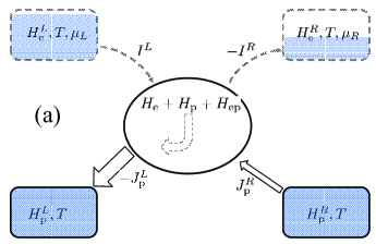
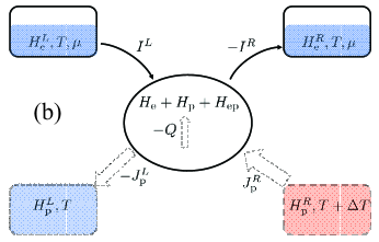
Figure 1: Schematic representation of the model system considered in this paper, and its different possible situations: (a) By applying a voltage bias, heat can be extracted from one of the phonon baths, although they remain at the same temperature. (b) By applying a temperature difference between the two phonon baths, an electrical current can be generated between the two electron baths. This contributes with a phonon-drag part to the thermopower.

II.2 Linear transport coefficients

In the linear response regime, we introduce an infinitesimal change of the chemical potential or temperature at one of the baths, $\alpha$, e.g., $\mu^{\alpha}=\mu+\delta\mu$, $T_{\sigma}^{\alpha}=T+\delta T_{\sigma}$, with $\mu$ and $T$ the corresponding equilibrium values. We look at the response of the charge and heat current due to this small perturbation. Up to the 2nd order in $M$, the result is summarized as follows

$$\left(\begin{array}[]{ccc}\frac{I^{\alpha}}{e}\\ J^{\alpha}_{\rm e}\\ J^{\alpha}_{\rm p}\end{array}\right)=\left(\begin{array}[]{ccc}\mathcal{L}_{0}&\mathcal{L}_{1}&\tilde{\mathcal{Q}}_{0}\\ \mathcal{L}_{1}&\mathcal{L}_{2}&\tilde{\mathcal{Q}}_{1}\\ {\mathcal{Q}}_{0}&{\mathcal{Q}}_{1}&\mathcal{K}_{\rm p}\\ \end{array}\right)\left(\begin{array}[]{ccc}\delta\mu\\ \frac{\delta T_{\rm e}}{T}\\ \frac{\delta T_{\rm p}}{T}\end{array}\right).$$ (4)

We define the positive current direction as that electrons/phonons go from the bath to the device, and $I^{\alpha}$, $J^{\alpha}_{\rm e}$, $J^{\alpha}_{\rm p}$ are the electrical current, heat current carried by electrons and phonons, respectively. The expressions for the coefficients $\mathcal{L}$ and $\mathcal{K}_{\rm p}$ are given in Appendix A. Both include three contributions. The first term is the elastic Landauer result. The second term is the (quasi-)elastic correction due to change of the electron spectral function. The last one is the inelastic term. The effect of each part in $\mathcal{L}$ on the conductance and Seebeck coefficient have been analyzed in Ref. Lü et al., 2015 for a single level model. $\mathcal{Q}_{n}$ and $\tilde{\mathcal{Q}}_{n}$ are the drag coefficients. We use the following convention for the drag effect: The electron drag effect corresponds to generating phonon flow due to electron flow, while the phonon drag corresponds to the opposite process. We can write $\mathcal{Q}_{n}$ and $\tilde{\mathcal{Q}}_{n}$ as

$$\tilde{\mathcal{Q}}_{n}\!\! = \!\!-\!\!\sum_{\beta}\!\!\int\!\!\frac{d\omega}{2\pi}\hbar\omega\textrm{Tr}[\Lambda^{(n)}_{\tilde{\alpha}\beta}(\omega)\mathcal{A}_{\alpha}(\omega)]\partial_{\hbar\omega}n_{B}(\hbar\omega,T),$$ (5)

$${\mathcal{Q}}_{n}\!\! = \!\!-\!\!\sum_{\beta}\!\!\int\!\!\frac{d\omega}{2\pi}\hbar\omega\textrm{Tr}[\Lambda^{(n)}_{\alpha\beta}(\omega)\tilde{\mathcal{A}}_{\alpha}(\omega)]\partial_{\hbar\omega}n_{B}(\hbar\omega,T),$$ (6)

where $n_{B}(\hbar\omega,T)=\left[{\rm exp}\left(\frac{\hbar\omega}{k_{B}T}\right)-1\right]^{-1}$ is the Bose-Einstein distribution function. Throughout the paper, we use ${\rm Tr}[\cdot]$ for trace over phonon indices, ${\rm tr}[\cdot]$ for trace over electronic degrees of freedom, $\tilde{\mathcal{A}}_{\alpha}/\mathcal{A}_{\alpha}$ is the (time-reversed) phonon spectral function [Eq. (46)], and $\Lambda^{(n)}_{\tilde{\alpha}\beta}(\omega)$ is defined as

$$\Lambda^{(n)}_{\tilde{\alpha}\beta}(\omega) = \int\frac{d\varepsilon}{2\pi}(\varepsilon-\mu_{0})^{n}X_{\tilde{\alpha}\beta}(\varepsilon,\varepsilon_{-})$$

$$\times \bigl{[}f(\varepsilon,\mu_{\alpha},T_{\alpha}^{e})-f(\varepsilon_{-},\mu_{\beta},T_{\beta}^{e})\bigr{]},$$

$$X_{\tilde{\alpha}\beta}(\varepsilon,\varepsilon_{-}) = \textrm{tr}\bigl{[}M\tilde{A}_{\alpha}(\varepsilon)MA_{\beta}(\varepsilon_{-})\bigr{]},$$ (8)

with $\varepsilon_{-}=\varepsilon-\hbar\omega$, and $\mu_{0}$ the equilibrium chemical potential. In the definition of $X_{\tilde{\alpha}\beta}$ and $\Lambda^{(n)}_{\tilde{\alpha}\beta}$, $\tilde{\alpha}$ means we need to use the time-reversed electron spectral function $\tilde{A}_{\alpha}$ [Eq. (45)]. $\Lambda^{(0)}(\omega)$ is the coupling-weighted electron-hole pair density of states (DOS), introduced in our previous workLü et al. (2010, 2012, 2015). In the linear regime, the Fermi distribution $f(\varepsilon,\mu_{\alpha},T^{\alpha})=f(\varepsilon,\mu,T)$ is the same for both electrodes, with $f(\varepsilon,\mu,T)=\left[{\rm exp}\left({\frac{\varepsilon-\mu}{k_{B}T}}\right)+1\right]^{-1}$. Hereafter, the summation of $\beta$ is over $L$ and $R$, and the integration is from $-\infty$ to $+\infty$ if not specified explicitly. In the linear regime, without magnetic field, we have $(D^{r})^{T}=D^{r}$ and $(G^{r})^{T}=G^{r}$. This leads to $\mathcal{Q}_{n}=\tilde{\mathcal{Q}}_{n}$, which ensures the Onsager symmetry (Appendix B).

For one electronic level coupled to one phonon mode, we can check that our result for $\mathcal{Q}_{0}/{\mathcal{Q}}_{1}$ is equivalent to that of Ref. Entin-Wohlman et al., 2010(Appendix C). In order for $\mathcal{Q}_{0}/{\mathcal{Q}}_{1}$ to be non-zero, we need some special design of the system, e.g., asymmetric coupling to the left and right electron bathEntin-Wohlman et al. (2010).

Here, we focus on the case where there are two or more phonon modes. For ${\tilde{\mathcal{Q}}}_{0}$, we can do an expansion over the energy dependence of the electron spectral function. The zeroth order contribution is

$$\tilde{\mathcal{Q}}_{0}^{(0)} = \sum_{\beta}\int\frac{d\omega}{4\pi^{2}}(\hbar\omega)^{2}\partial_{\hbar\omega}n_{B}(\hbar\omega,T)$$

$$\times \textrm{Tr}[{\rm Im}X_{\tilde{\alpha}\beta}(\mu,\mu){\rm Im}{\mathcal{A}}_{\alpha}(\omega)],$$

with Re and Im meaning real and imaginary part, respectively. In order for $\tilde{\mathcal{Q}}_{0}^{(0)}$ to be non-zero, the device needs to have at least two vibrational modes. This follows from the fact that $\mathcal{A}_{\alpha}$ is Hermitian.

II.2.1 Relation with adiabatic pumping and current-induced forces

Now we write $\tilde{\mathcal{Q}}_{0}^{(0)}$ in terms of the unperturbed retarded (advanced) electron scattering states, coming from (leaving to) the left $|\psi_{L}\rangle$ ($|\tilde{\psi}_{L}\rangle$) or right $|\psi_{R}\rangle$ ($|\tilde{\psi}_{R}\rangle$) electrode

$$X^{kl}_{\tilde{\alpha}\beta}(\varepsilon,\varepsilon_{-}) = \sum_{m,n}\langle\psi_{\beta}^{n}(\varepsilon_{-})|M^{k}|\tilde{\psi}_{\alpha}^{m}(\varepsilon)\rangle\langle\tilde{\psi}^{m}_{\alpha}(\varepsilon)|M^{l}|\psi_{\beta}^{n}(\varepsilon_{-})\rangle.$$

Here, $m$ and $n$ are channel indices. The retarded and advanced scattering states including e-ph interaction are generated from

$$|\Psi_{\alpha}(\varepsilon)\rangle = |\psi_{\alpha}(\varepsilon)\rangle+G^{r}H_{\rm ep}|\psi_{\alpha}(\varepsilon)\rangle,$$ (11)

$$|\tilde{\Psi}_{\alpha}(\varepsilon)\rangle = |\psi_{\alpha}(\varepsilon)\rangle+G^{a}H_{\rm ep}|\psi_{\alpha}(\varepsilon)\rangle,$$ (12)

They are normalized as

$$\langle\Psi_{\alpha}(\varepsilon)|\Psi_{\beta}(\varepsilon^{\prime})\rangle=2\pi\delta(\alpha,\beta)\delta(\varepsilon-\varepsilon^{\prime}),$$ (13)

and so is $|\psi_{\alpha}\rangle$. From the definition of the scattering matrix

$$2\pi\delta(\varepsilon-\varepsilon^{\prime})S_{\alpha\beta}^{mn}=\langle\tilde{\Psi}_{\alpha}^{m}(\varepsilon^{\prime})|\Psi_{\beta}^{n}(\varepsilon)\rangle,$$ (14)

and Eqs. (11-12), we get

$$S_{\alpha\beta}^{mn}=\delta_{\alpha,\beta}\delta_{m,n}-i\langle{\psi}_{\alpha}^{m}|H_{\rm ep}|\Psi_{\beta}^{n}\rangle.$$ (15)

Here, $S_{\alpha\beta}^{mn}$ is the matrix element connecting the incoming wave from the $n$-th channel in electrode $\beta$ to the $m$-th outgoing channel in electrode $\alpha$. Taking the derivative over the phonon displacement yields

$$\partial_{k}S_{\alpha\beta}^{mn}=-i\langle\tilde{\Psi}_{\alpha}^{m}|M^{k}|\Psi_{\beta}^{n}\rangle.$$ (16)

Substituting Eq. (16) into Eq. (II.2.1), taking the $\omega\to 0$ limit, we obtain

$${\rm Im}\sum_{\beta}{\rm tr}\bigl{[}\partial_{l}S_{\alpha\beta}\partial_{k}S_{\beta\alpha}^{\dagger}\bigr{]}={\rm Im}\sum_{\beta}X_{\tilde{\alpha}\beta}^{kl}+\cdots.$$ (17)

The trace is over the channel indices. We have kept only the second order terms.

Equation (17) makes connection with the Brouwer formula for adiabatic pumpingBrouwer (1998); Thomas et al. (2012); Bustos-Marún et al. (2013). Here, a temperature difference between the left and right electrode breaks the population balance between the phonon scattering states from these two baths, e.g., there are more phonon waves travelling in one direction, determined by the temperature bias. When the phonon wave goes through the device, it produces phase-shifted oscillating potential felt by the electrons. In the space of the atomic coordinates, the trajectory may form a closed loop, generating pumped electrical current.

The opposite of this effect is that an electrical current generates a directed phonon heat current. The term governing this effect is $X_{LR}$. The same term appears in the expressions for the current-induced nonconservative and effective magnetic forcesDundas et al. (2009); Lü et al. (2010); Bode et al. (2011); Todorov et al. (2011); Lü et al. (2012), e.g., Eqs. (56-61) in Ref. Lü et al., 2012. This shows that the electron drag effect is closely related to these novel current-induced forces.

II.3 Nonlinear regime

When the applied temperature or voltage bias is large, additional energy transfer between the electron and phonon subsystem takes place. We consider two situations: Electrical-current-driven heat flow in the isothermal case, and temperature-driven electrical current at zero voltage bias.

II.3.1 Electrical current induced heat flow
($T^{e}=T^{\rm p}=T$, $eV\neq 0$)

In the first setup, all the baths are at the same temperature ($T$), but the electron baths are subject to a nonzero voltage bias ($eV=\mu_{L}-\mu_{R}$). This is the most common situation in a working electronic device [Fig. 1 (a)]. For large bias, there will be energy transfer from the electron to the phonon subsystem

$$Q\! = \!\!2\sum_{\alpha,\beta}\int\frac{d\omega}{2\pi}\int\frac{d\varepsilon}{2\pi}\hbar\omega{\rm Tr}\left[{\rm tr}\left[MA_{\alpha}(\varepsilon)MA_{\beta}(\varepsilon+\hbar\omega)\right]\mathcal{A}(\omega)\right]$$ (18)

$$\times f_{\beta}(\varepsilon+\hbar\omega)(1-f_{\alpha}(\varepsilon))(n_{B}(\hbar\omega,T)+1).$$

Since all the baths are at the same temperature, we have omitted it in this subsection. Equation (18) is a result of balance between phonon emission and adsorption processes [Fig. 2]. For $\omega>0$, it represents process where an electron in electrode $\beta$ combines with a hole at lower energy in $\alpha$, accompanied by a phonon emission process. For $\omega<0$, it represents the opposite process, where an electron-hole pair is created between $\alpha$ and $\beta$ by adsorbing one phonon. While the Fermi distributions $f_{\beta}(1-f_{\alpha})$ ensures that the phonon emission process happens only when the applied bias $eV$ is larger than the phonon energy $\hbar\omega$, the Bose function $n_{B}+1$ prohibits phonon adsorption process at $T=0$. This equation can also be written in a compact form as

$$Q\! = \!\!\int\frac{d\omega}{2\pi}\hbar\omega{\rm Tr}\bigl{[}\Lambda^{(0)}_{LR}(\omega){\mathcal{A}}(\omega)\bigr{]}\Delta n_{B}(\hbar\omega,T;\hbar\omega-eV,T),$$

with

$$\Delta n_{B}(\hbar\omega_{1},T_{1};\hbar\omega_{2},T_{2})=n_{B}(\hbar\omega_{1},T_{1})-n_{B}(\hbar\omega_{2},T_{2}).$$ (20)

Energy transfer within the device breaks the balance between the device and bath phonons. As a result, the extra energy is further transferred to the two phonon baths. The heat current flowing out of the phonon bath $\alpha$ is given by the minus of Eq. (LABEL:eq:power) with $\tilde{\mathcal{A}}$ replaced by $\tilde{\mathcal{A}}_{\alpha}$, such that

$$J_{\rm p}^{L}+J_{\rm p}^{R}+Q=0,$$ (21)

as required by the energy conservation.

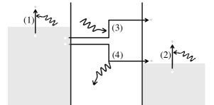
Figure 2: Electron-hole pair excitation and recombination processes. (1) and (2) are intra-electrode processes. (3) and (4) are inter-electrode ones. At $T=0$, (1)-(3) are not possible, and (4) is possible only when the applied bias is larger than the phonon energy.

In fact, we can split $J_{\rm p}^{\alpha}$ into two parts according to their symmetry upon bias reversal $J_{\rm p}^{\alpha}=J_{\rm p}^{\alpha,h}+J_{\rm p}^{\alpha,p}$, where $J_{\rm p}^{\alpha,h}$ and $J_{\rm p}^{\alpha,p}$ are even and odd function of $eV$. We call them the Joule heating and Peltier drag current, respectively. Assuming constant electron DOS, we get

$$J_{\rm p}^{\alpha,h}\!\! \approx \!\!-\!\!\int_{0}^{+\infty}\frac{d\omega}{4\pi^{2}}\;h(\hbar\omega){\rm{Tr}}[{\rm Re}X_{LR}(\mu,\mu){\rm Re}\tilde{\mathcal{A}}_{\alpha}(\omega)],$$

$$J_{\rm p}^{\alpha,p}\!\! \approx \!\!-\!\!\int_{0}^{+\infty}\frac{d\omega}{4\pi^{2}}\;p(\hbar\omega){\rm Tr}[{\rm Im}X_{LR}(\mu,\mu){\rm Im}\tilde{\mathcal{A}}_{\alpha}(\omega)].$$

The two coefficients are

$$h(\hbar\omega)\!\! \equiv \!\!\sum_{s=\pm 1}\!\!\hbar\omega(\hbar\omega+s\,eV)\Delta n_{B}(\hbar\omega+seV;\hbar\omega),$$ (24)

$$p(\hbar\omega)\!\! \equiv \!\!\sum_{s=\pm 1}\!\!s\,\hbar\omega(\hbar\omega+s\,eV)\Delta n_{B}(\hbar\omega+seV;\hbar\omega).$$ (25)

The Joule current corresponds to the energy transfer from the electrons to the phonons in Eq. (LABEL:eq:power), i.e., $J_{\rm p}^{L,h}+J_{\rm p}^{R,h}+Q=0$. But the drag current is related to the $\mathcal{Q}_{0}$ coefficient in Subsec. II.2, and depends on the direction of current flow, i.e., $J_{\rm p}^{L,p}+J_{\rm p}^{R,p}=0$. This relation follows from the fact that ${\rm Im}\mathcal{A}={\rm Im}\tilde{\mathcal{A}}={\rm Im}\tilde{\mathcal{A}}_{L}+{\rm Im}\tilde{\mathcal{A}}_{R}=0$. We will see later that it is due to momentum transfer between electrons and phonons. In the limit of high temperature ($k_{B}T\gg eV\pm\hbar\omega$), we have $h(\hbar\omega)\to 0$, and $p(\hbar\omega)\to 2eVk_{B}T$. The drag part will dominate over the Joule heating part. In this case, it is possible to extract heat from one of the phonon baths by applying a voltage bias, similar to a refrigerator, as shown in Fig. 1 (b).

We note that in Ref. Lü et al., 2015, we have studied the same problem using the semi-classical generalized Langevin equation approach. Similar equations were derived there, and the asymmetric heat flow was attributed to the asymmetric current-induced forces. These two complementary analysis shows that the two effects are closely related.

II.3.2 Temperature-driven electric current
($\mu_{L}=\mu_{R}$,$T^{e}\neq T^{\rm p}$)

In the second setup, we apply a temperature difference between the electron and phonon subsystem at zero voltage bias. This drives an electrical current within the device

$${I}^{\alpha}=e\sum_{\beta}\int\frac{d\omega}{2\pi}{\textrm{Tr}}\bigl{[}\Lambda^{(0)}_{\tilde{\alpha}\tilde{\bar{\alpha}}}(\omega)\mathcal{A}_{\beta}(\omega)\bigr{]}\Delta n_{B}(\hbar\omega,T_{\rm p}^{\beta};\hbar\omega,T_{\rm e}).$$

(26)

Here, $\bar{\alpha}$ means the lead different from $\alpha$. There are two possible situations here. The first one is that the phonon baths are at the same temperature ($T_{\rm p}$), but different from that of electron baths ($T_{\rm e}$). We can consider the two phonon baths as an effective single bath. The four-terminal setup reduces to a three-terminal one, and equation (26) simplifies to

$${I}^{\alpha}=e\int\frac{d\omega}{2\pi}{\textrm{Tr}}\left[\Lambda^{(0)}_{\tilde{\alpha}\tilde{\bar{\alpha}}}(\omega)\mathcal{A}(\omega)\right]\Delta n_{B}(\hbar\omega,T_{\rm p};\hbar\omega,T_{\rm e}).$$ (27)

The three-terminal setup has been considered in Ref. Entin-Wohlman et al., 2010. For a single electronic level coupling to one phonon mode, equation (27) agrees with result therein. Due to the temperature difference between the electron and phonon systems, there will be energy flow between them. It has been analyzed in Sec. III C of Ref. Lü et al., 2015. A similar problem has been considered in Refs. Segal, 2008; Zhang et al., 2013; Ren and Zhu, 2013; Vinkler-Aviv et al., 2014. Here we focus on the other situation, where we apply a temperature difference between the two phonon baths [Fig. 1 (b)]. This generates a phonon-drag electrical current. For constant electronic DOS, we get

$${I}^{\alpha}\approx e\int\frac{d\omega}{4\pi^{2}} \hbar\omega {\textrm{Tr}}\left[{\rm Im}X_{\tilde{\alpha}\tilde{\bar{\alpha}}}(\mu,\mu){\rm Im}\mathcal{A}_{\bar{\alpha}}(\omega)\right]$$ (28)

$$\times \Delta n_{B}(\hbar\omega,T_{\rm p}^{\alpha};\hbar\omega,T_{\rm p}^{\bar{\alpha}}),$$

extending the result in Subsec. II.2 to the nonlinear regime.

III Model Calculation

III.1 1D model and qualitative analysis

For the ease of understanding the general results in Sec. II, we now study a simple 1D atomic chain. The electronic Hamiltonian takes the tight-binding form, with the hopping matrix element $-t$,

$$H_{\rm e}=-t\sum_{|i-j|=1}(c^{\dagger}_{i}c_{j}+{\rm h.c.}).$$ (29)

The electron dispersion relation is $\varepsilon_{k}=-2t\cos k$, where $k$ is the 1D wavevector[Fig. 3 (d)]. We have set the lattice distance $a=1$. For this 1D lattice, due to translational invariance, the electron Green’s function in real space only depends on the distance between different sites $j$ and $l$, $n=j-l$,

$$G_{0,jl}^{r}(\varepsilon)=\frac{e^{i|k(\varepsilon^{+})n|}}{2it|\sin k(\varepsilon^{+})|}.$$ (30)

Here, $k(\varepsilon^{+})$ is the wavevector corresponding to energy $\varepsilon^{+}=\varepsilon+i0^{+}$. The left and right spectral function, defined within the electron energy band, are

$$A_{L,jl}(\varepsilon)=\tilde{A}^{*}_{L,jl}(\varepsilon)=\frac{e^{ik(\varepsilon^{+})n}}{2t|\sin k(\varepsilon^{+})|},A_{R}(\varepsilon)=A_{L}^{*}(\varepsilon).$$

(31)

The ions are connected by 1D springs with spring constant $K_{0}$

$$H_{\rm p}=\sum_{j}\left(\frac{1}{2}{\dot{u}}_{j}^{2}+K_{0}{u}_{j}^{2}\right)-\frac{1}{2}K_{0}\sum_{|i-j|=1}{u}_{i}{u}_{j},$$ (32)

The phonon retarded Green’s function is

$$D^{r}_{0,jl}(\omega)=\frac{e^{i|q(\omega^{+})n|}}{2iK_{0}|\sin q(\omega^{+})|}.$$ (33)

Here, $q(\omega^{+})$ is the phonon wavevector corresponding to frequency $\omega^{+}=\omega+i0^{+}$, which we can get from the dispersion relation $\omega_{q}=2\sqrt{K_{0}}\left|\sin\frac{q}{2}\right|$ [Fig. 3 (c)]. The phonon spectral function, defined within the phonon band, is

$$\mathcal{A}_{L,jl}(\omega)=\mathcal{\tilde{A}}_{L,jl}^{*}(\omega)=\frac{e^{iq(\omega^{+})n}}{2K_{0}|\sin q(\omega^{+})|},\mathcal{A}_{R}(\omega)=\mathcal{A}_{L}^{*}(\omega).$$ (34)

To consider the e-ph interaction, we assume the atomic motion modifies the hopping matrix element linearly, i.e.,

$$H_{\rm ep}=-m\sum_{j}{u}_{j}(c^{\dagger}_{j}c_{j+1}-c^{\dagger}_{j}c_{j-1}+{\rm h.c.}).$$ (35)

For a phonon emission process through electronic transition from the initial left scattering states $|\psi_{L}(k_{L})\rangle$ to the final right scattering state $|\psi_{R}(k_{R})\rangle$, only phonon mode that fulfills the energy and crystal-momentum conservation can be excited, e.g., $\langle\psi_{L}(k_{L})|M^{q}|\psi_{R}(k_{R})\rangle\sim\delta(k_{L}-k_{R}-q+G)\delta\bigl{(}\varepsilon(k_{L})-\varepsilon(k_{R})-\hbar\omega(q)\bigr{)}$. Here, $G$ is a reciprocal lattice vector, and $k_{L}>0$, $k_{R}<0$. It is this selection rule that gives the electron/phonon drag effect in a translational invariant lattice[Fig. 3 (c)-(d)].

To show that similar mechanism works in a coherent nano-conductor, we artificially switch off the e-ph interaction, except at two sites, e.g., we only consider coupling to $u_{n}$ and $u_{n+1}$[Fig. 3 (b)]. That is, in Eq. (35), the sum over $j$ only applies to these two sites. Then, only nearest hopping between four sites, $\{n-1,n,n+1,n+2\}$, are modified by atomic motion. We set these four sites as our device, and all other sites as electron and phonon baths $L$ and $R$. In this case, the condition of energy conservation is still valid, but the conservation of crystal-momentum is not, since the local e-ph interaction breaks the translation invariance. The matrix element is

$$\langle\psi_{L}(k_{L})|M^{q}|\psi_{R}(k_{R})\rangle = -\frac{m}{\hbar\sqrt{|v_{L}v_{R}|}}e^{-ik_{L}}\left[1+e^{i(q-k_{L}+k_{R})}\right]\left[1+e^{i(k_{L}+k_{R})}\right]\left[1-e^{-i(k_{L}-k_{R})}\right].$$ (36)

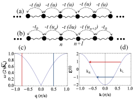
Figure 3: (a) A model 1D lattice, where the electron nearest-neighbor hopping amplitude $t(u)$ depends on the atomic displacement $u$. (b)Localized e-ph interaction at sites $n$ and $n+1$, $\delta u=u_{n+1}-u_{n}$. (c) Phonon dispersion relation. (d) Electron dispersion relation. Blue and red lines depict phonon emission processes due to e-ph interaction. An electron at state $k_{L}$ is scattered by phonons to an state $k_{R}$ and emit one phonon, whose wavevector is denoted by the vertical lines in (c). Depending on the value of $k_{L}$ and $k_{R}$, the emitted phonon may travel to the right (blue line, normal process) or the left (red line, Umklapp process). Normally, the electron energy is much larger than the phonon energy, so in this figure we have ignored the electron energy change.

Here, $v_{L/R}$ is the group velocity of the $L/R$ scattering state with wavevector $k_{L/R}$. We can see that the squared scattering matrix element $|\langle\psi_{L}(q_{L})|M^{q}|\psi_{R}(q_{R})\rangle|^{2}\neq|\langle\psi_{L}(q_{L})|M^{-q}|\psi_{R}(q_{R})\rangle|^{2}$, their difference

$$\Delta M_{LR}\propto\sin\phi\sin q.$$ (37)

We have defined $\phi=k_{L}-k_{R}$. This means the electrons have different probability of exciting left and right traveling phonon waves. The difference depends on the electron and phonon wavevectors. For example, similar to the 1D lattice, electrons with $\varepsilon<0$ (below half filling) preferentially emit phonons travelling to the right. From another point of view, the holes dominate the inelastic transportLü et al. (2015). This breaks the left-right symmetry, and generates drag effect in a nano-conductor, although the crystal-momentum selection rule is not valid.

To make connection with the NEGF approach in Sec. II, we can calculate the real space e-ph interaction matrix at sites $n$ and $n+1$, and find $M^{n+1}_{LR}\equiv\langle\psi_{L}(k_{L})|M^{n+1}|\psi_{R}(k_{R})\rangle=e^{-i\phi}\langle\psi_{L}(k_{L})|M^{n}|\psi_{R}(k_{R})\rangle$. So,

$$X^{n,n+1}_{LR}\bigl{(}\varepsilon(k_{L}),\varepsilon(k_{R})\bigr{)}=\left|M^{n}_{LR}\right|^{2}\left(\begin{array}[]{cr}1&e^{-i\phi}\\ e^{i\phi}&1\\ \end{array}\right).$$ (40)

Making use of Eq. (34), we get, for given electron ($k_{L}$, $k_{R}$) and phonon wavevectors ($q$), that satisfy the requirement of energy conservation, $\varepsilon(k_{L})=\varepsilon(k_{R})+\hbar\omega(q)$, the electron ‘drag’ term becomes,

$${\rm Tr}\bigl{[}{\rm Im}X_{LR}(\omega){\rm Im}\tilde{\mathcal{A}}_{L}(\omega)\bigr{]}\propto\sin\phi\sin q(\omega^{+}).$$ (41)

This is consistent with our scattering analysis, and shows that the drag effect we discuss here shares the same origin as that in lattice system.

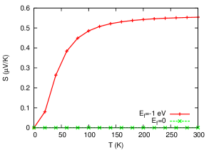
Figure 4: Phonon drag contribution to the Seebeck coefficient at different chemical potentials. The parameters used are as follows: $t=1$ eV, $K_{0}=0.02$ eV/(Ųu), $K^{\prime}_{0}=0.5K$, $m=0.15$ eV/(Å$\sqrt{{\rm u}}$). Here, $K^{\prime}_{0}$ is the spring constant connecting the device to the left and right phonon baths.

III.2 Numerical results

Now we present our numerical results for the 1D model with localized e-ph interaction using the formulas developed in Sec. II. In Fig. 4, we show the calculated phonon drag contribution to the Seebeck coefficient. The parameters, given in the figure caption, are chosen to closely resemble that of a single atom gold chainde la Vega et al. (2006); Ludoph and van Ruitenbeek (1999); Matsushita et al. (2015); Evangeli et al. (2015). The single electron contribution to the Seebeck coefficient vanishes, since we have a perfect electron transport channel. The drag coefficient is zero at $E_{F}=0$ due to electron-hole symmetryLü et al. (2015). But once moving to $E_{F}=-1$ eV, the symmetry is broken, and we get a non-zero value. Positive $S$ means the holes dominate over the electrons in the inelastic scattering process. The saturation of the $S$ with $T$ can be understood from Eq. (II.2), i.e., at high temperature, $\tilde{\mathcal{Q}}_{0}\propto T$, while $S\propto\tilde{\mathcal{Q}}_{0}/T$.

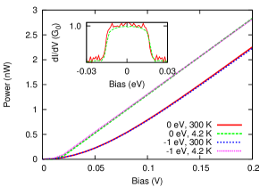
Figure 5: Energy current going from electron to phonons (power) as a function of voltage bias at different temperatures and Fermi levels from Eqs. (LABEL:eq:power-21). All the electron and phonon baths are kept at the same temperature, see also Fig. 1 (b). The inset shows the differential conductance ($dI/dV$) at $E_{F}=0$ (red, solid) and $-1$ eV (green, dashed) at $4.2$ K.

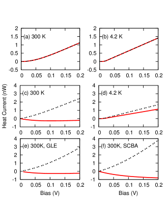
Figure 6: Heat current carried by phonons, going into the left (red, solid) and right (black, dashed) phonon bath. (a)-(b) $E_{F}=0$, (c)-(f) $E_{F}=-1$ eV. (a)-(d) Calculated from Eqs. (LABEL:eq:power-21). We also show the results calculated from the generalized Langevin equation (GLE) approach (Ref. Lü et al., 2012) (e) and the self-consistent Born approximation (SCBA) (Ref. Lü and Wang, 2007) (f).

Figures 5-6 show the results for the setup in Fig. 1 (a). The temperatures of all the baths are the same, while there is a voltage bias applied between the two electron baths. We define the power as Q in Eq. (LABEL:eq:power). Figure 5 shows its dependence on the voltage bias at different temperatures and Fermi levels. The onset of power flow at the phonon frequency is clear at $4.2$ K, but smoothed out at $300$ K. The inset shows the corresponding conductance drop at the phonon threshold for $4.2$ K. Although the magnitude of the power changes slightly, the general behavior does not depend on the position of the Fermi level. All these results agree with previous studiesFrederiksen et al. (2004); Viljas et al. (2005); Lü and Wang (2007).

Next, we show in Fig. 6(a) and (b) that the heat flows into the left and right phonon baths are drastically different at the two Fermi levels. For $E_{F}=0$, the heat flow into the two phonon baths are symmetric (Fig. 6 (a-b)). But when we move to $E_{F}=-1.0$ eV, they show strong asymmetry, due to the drag part of the heat current (Fig. 6 (c-d)). It depends on the phase of the electron wavefunction, which in our case could be tuned by changing the chemical potential. At $E_{F}=-1$ eV, the probability of emitting right travelling phonons is larger, resulting in larger heat current into bath $R$. This is the same with the lattice system [Fig. 3 (c)-(d)]. Comparing results at $T=4.2$ and $300$ K, we find that the asymmetry increases with temperature. Interestingly, at $300$ K, we can extract heat from the right phonon bath by applying the voltage bias. This is a prototype atomic ‘refrigerator’. The results calculated using the generalized Langevin equation (GLE) approachLü et al. (2012)[Fig. 6 (e)] and self-consistent Born approximation (SCBA)Lü and Wang (2007)[Fig. 6 (f)] show that, although the magnitude of the heat current changes, the qualitative conclusions remain no matter which approximation we use.

IV Conclusions

In conclusion, by assuming linear coupling between electron and phonons in a four-terminal nano-device, we have shown that in the linear transport regime, in addition to modifying the normal thermoelectric transport coefficients, e-ph interaction also introduces new drag type coefficients. The drag effect can be traced back to the momentum transfer between the electrons and phonons. We have shown that it is closely related to the adiabatic pumping, and current-induced forces in a coherent conductor. So in principle phonon-drag thermopower behaves as an alternative way of probing these current-induced forces. The expressions derived in this paper can be readily applied to the realistic structures by combining these with first-principles electronic structure calculationSoler et al. (2002); Brandbyge et al. (2002); Frederiksen et al. (2007). Finally, we note that one could also study similar drag effect in coulomb coupled all-electronic devicesSánchez et al. (2010); Sothmann et al. (2012); Whitney et al. (2016).

Appendix A Expressions for $\mathcal{L}$ and $\mathcal{K}_{\rm p}$

We write down the full expressions for the thermoelectric coefficients in Eq. (4). The complete $\mathcal{L}$ including e-ph interaction is made from three contributions:

$$\mathcal{L}_{n}=\sum_{i=1}^{3}\mathcal{L}^{(i)}_{n},$$ (42)

with

$$\mathcal{L}^{(1)}_{n} = \frac{1}{\hbar}\int\frac{d\varepsilon}{2\pi}(\varepsilon-\mu)^{n}\textrm{tr}\left[A_{\bar{\alpha}}(\varepsilon)\Gamma_{\alpha}(\varepsilon)\right]f^{\prime}(\varepsilon),\quad\mathcal{L}^{(2)}_{n}=\frac{1}{\hbar}\int\frac{d\varepsilon}{2\pi}(\varepsilon-\mu)^{n}\textrm{tr}\left[\Delta A_{\bar{\alpha}}(\varepsilon)\Gamma_{\alpha}(\varepsilon)\right]f^{\prime}(\varepsilon),$$ (43)

$$\mathcal{L}^{(3)}_{n} = \frac{i}{\hbar}\int\frac{d\varepsilon}{2\pi}(\varepsilon-\mu)^{n}{\rm tr}\bigl{[}(\Sigma_{\rm ep}^{>}(\varepsilon)-\Sigma_{\rm ep}^{<}(\varepsilon))\tilde{A}_{\alpha}(\varepsilon)\bigr{]}f^{\prime}(\varepsilon).$$ (44)

We have defined $f^{\prime}(\varepsilon)=-\frac{\partial f(\varepsilon,\mu,T)}{\partial\varepsilon}$. Since the chemical potential $\mu$ and temperature $T$ are all the same for both electrodes. We have omitted them to simplify the expressions. We also have

$$A_{\alpha}(\varepsilon)=G_{0}^{r}(\varepsilon)\Gamma^{e}_{\alpha}(\varepsilon)G_{0}^{a}(\varepsilon),\quad\tilde{A}_{\alpha}(\varepsilon)=G_{0}^{a}(\varepsilon)\Gamma^{e}_{\alpha}(\varepsilon)G_{0}^{r}(\varepsilon),\quad A(\omega)=A_{L}(\omega)+A_{R}(\omega),$$ (45)

$${\mathcal{A}}_{\alpha}(\omega)=D_{0}^{r}(\omega)\Gamma^{\rm p}_{\alpha}(\omega)D_{0}^{a}(\omega),\quad\tilde{\mathcal{A}}_{\alpha}(\omega)=D_{0}^{a}(\omega)\Gamma^{\rm p}_{\alpha}(\omega)D_{0}^{r}(\omega),\quad\mathcal{A}(\omega)=\mathcal{A}_{L}(\omega)+\mathcal{A}_{R}(\omega).$$ (46)

$\mathcal{L}^{(1)}_{n}$ is the single electron Landauer result. $\mathcal{L}^{(2)}_{n}$ is due to corrections to the electron DOS

$$\Delta A_{\bar{\alpha}}=G^{r}_{0}(\varepsilon)\Sigma_{\rm ep}^{r}(\varepsilon)A_{\bar{\alpha}}(\varepsilon)+A_{\bar{\alpha}}(\varepsilon)\Sigma_{\rm ep}^{a}(\varepsilon)G_{0}^{a}(\varepsilon).$$ (47)

$\mathcal{L}^{(3)}$ is the inelastic term. Note that only the Fock diagram contributes to $\mathcal{L}^{(3)}$. Effect of e-ph interaction on the $\mathcal{L}_{n}$ in a single level model has been studied in Ref. Lü et al., 2015.

The phonon thermal conductance has similar form

$$\mathcal{K}_{\rm p}=\sum_{i=1}^{3}\mathcal{K}^{(i)}_{\rm p}$$ (48)

with

$$\mathcal{K}^{(1)}_{\rm p} = \int\frac{d\omega}{4\pi}\hbar\omega\textrm{Tr}\left[\mathcal{A}_{\bar{\alpha}}(\omega)\Gamma_{\rm p}^{\alpha}(\omega)\right]\frac{\partial n_{B}}{\partial T_{\rm p}}T_{\rm p},\quad\mathcal{K}^{(2)}_{\rm p}=\int\frac{d\omega}{4\pi}\hbar\omega\textrm{Tr}\left[\Delta\mathcal{A}_{\bar{\alpha}}(\omega)\Gamma_{\rm p}^{\alpha}(\omega)\right]\frac{\partial n_{B}}{\partial T_{\rm p}}T_{\rm p},$$ (49)

$$\mathcal{K}^{(3)}_{\rm p} = i\int\frac{d\omega}{4\pi}\hbar\omega\textrm{Tr}\left[(\Pi_{\rm ep}^{>}(\omega)-\Pi_{\rm ep}^{<}(\omega))\tilde{\mathcal{A}}_{\alpha}(\omega)\right]\frac{\partial n_{B}}{\partial T_{\rm p}}T_{\rm p}.$$ (50)

Here $\bar{\alpha}$ means electrode opposite to $\alpha$. Similarly, $\mathcal{K}^{(2)}_{n}$ is due to corrections to the phonon DOS

$$\Delta\mathcal{A}_{\bar{\alpha}}=D^{r}_{0}(\varepsilon)\Pi_{\rm ep}^{r}(\varepsilon)\mathcal{A}_{\bar{\alpha}}(\varepsilon)+\mathcal{A}_{\bar{\alpha}}(\varepsilon)\Pi_{\rm ep}^{a}(\varepsilon)D_{0}^{a}(\varepsilon).$$ (51)

Appendix B Onsager symmetry

Here, we show that $\mathcal{Q}_{n}=\tilde{\mathcal{Q}}_{n}$ in the presence of time-reversal symmetry, e.g., $(G^{r})^{T}=G^{r}$. In that case, from Eq. (46), we have

$$\tilde{\mathcal{A}}_{\alpha}=\mathcal{A}_{\alpha}^{*},\quad\tilde{\mathcal{A}}=\mathcal{A},\quad\tilde{{A}}_{\alpha}={A}_{\alpha}^{*},\quad\tilde{A}=A.$$ (52)

Furthermore, $A$ and $\mathcal{A}$ are both real. Consequently, in the linear response regime, we can set $f(\varepsilon,\mu_{\alpha},T_{\alpha})=f(\varepsilon,\mu_{\beta},T_{\beta})$ in Eq. (II.2), and get

$$\sum_{\beta}\Lambda_{\tilde{\alpha}\beta}^{(n)}=\sum_{\beta}\Lambda_{\tilde{\alpha}\tilde{\beta}}^{(n)}=\big{(}\sum_{\beta}\Lambda_{{\alpha}{\beta}}^{(n)}\big{)}^{*}.$$ (53)

Using the above two equations, we see that $\mathcal{Q}_{n}^{*}=\tilde{\mathcal{Q}}_{n}$.

On the other hand, the coefficients $\mathcal{Q}_{n}$ are real $\mathcal{Q}_{n}=\mathcal{Q}_{n}^{*}$. This can be seen from the fact that: (1) the matrices $M$, $A$, $\mathcal{A}$ are real, and $A_{\alpha}/\mathcal{A}_{\alpha}$ is Hermitian; (2) the trace of their products is real. Putting them together, we get the desired result $\mathcal{Q}_{n}=\tilde{\mathcal{Q}}_{n}$.

Appendix C Equivalence to the results of Ref. 38

Here, we show that results of Ref. Entin-Wohlman et al., 2010 (Eqs. (35-36)) are special case of our results. There, the authors considered one electronic level at ($\varepsilon_{0}$) coupled to one vibrational mode with angular frequency $\omega_{0}$. The electronic level couples to two electrodes and the vibrational mode couples to one phonon bath, characterized by $\gamma_{ph}$. In this special case, all the matrices become numbers. We get $G_{0}^{r}(\varepsilon)=\left[\varepsilon+i\gamma(\varepsilon)/2-\varepsilon_{0}\right]^{-1}$, with $\gamma(\varepsilon)=\gamma_{R}(\varepsilon)+\gamma_{L}(\varepsilon)$, and $D_{0}^{r}(\omega)=\left[(\omega+i\gamma_{\rm ph})^{2}-\omega_{0}^{2}\right]^{-1}$. Now we have $\mathcal{Q}_{0}=0$, since the phonon mode couples only to one bath and $\mathcal{A}_{\alpha}$ is real. Substituting these two equations to Eq. (6), and assuming $\gamma_{\rm ph}$ is small, we get

$$\mathcal{Q}_{n} = m^{2}\int\frac{d\varepsilon}{4\pi}(\varepsilon+{\hbar\omega_{0}}/{2}-\mu)^{n}{|G^{r}_{0}(\varepsilon+\hbar\omega_{0}/2)|^{2}|G^{r}_{0}(\varepsilon-\hbar\omega_{0}/2)|^{2}}$$

$$\times \partial_{\hbar\omega}n_{B}(\hbar\omega_{0})\left[\gamma_{\alpha}(\varepsilon-\hbar\omega_{0}/2)\gamma_{\bar{\alpha}}(\varepsilon+\hbar\omega_{0}/2)-\gamma_{\alpha}(\varepsilon+\hbar\omega_{0}/2)\gamma_{\bar{\alpha}}(\varepsilon-\hbar\omega_{0}/2)\right](f(\varepsilon+\hbar\omega_{0}/2)-f(\varepsilon-\hbar\omega_{0}/2)).$$

This is consistent with Eqs. (35-36) of Ref. Entin-Wohlman et al., 2010. The extra factor $1/2$ in Eq. (C) comes from different definition of the e-ph interaction $m$. Note that we need $\gamma_{\alpha}(\varepsilon)$ to be energy dependent, and $\gamma_{\alpha}(\varepsilon)\neq\gamma_{\bar{\alpha}}(\varepsilon)$, in order for $\mathcal{Q}_{n}\neq 0$.

References

- Dresselhaus et al. (2007) M. S. Dresselhaus, G. Chen, M. Y. Tang, R. G. Yang, H. Lee, D. Z. Wang, Z. F. Ren, J. P. Fleurial, and P. Gogna, Adv. Mater. 19, 1043 (2007).
- Snyder and Toberer (2008) G. J. Snyder and E. S. Toberer, Nat. Mater. 7, 105 (2008).
- Majumdar (2004) A. Majumdar, Science 303, 777 (2004).
- Mahan and Sofo (1996) G. D. Mahan and J. O. Sofo, Proc. Natl. Acad. Sci. 93, 7436 (1996).
- Godijn et al. (1999) S. F. Godijn, S. Möller, H. Buhmann, L. W. Molenkamp, and S. A. van Langen, Phys. Rev. Lett. 82, 2927 (1999).
- Paulsson and Datta (2003) M. Paulsson and S. Datta, Phys. Rev. B 67, 241403 (2003).
- Reddy et al. (2007) P. Reddy, S. Jang, R. A. Segalman, and A. Majumdar, Science 315, 1568 (2007).
- Wang et al. (2008) J.-S. Wang, J. Wang, and J.-T. Lü, Euro. Phys. J. B 62, 381 (2008).
- Baheti et al. (2008) K. Baheti, J. A. Malen, P. Doak, P. Reddy, S. Jang, T. D. Tilley, A. Majumdar, and R. A. Segalman, Nano Lett. 8, 715 (2008).
- Dubi and Di Ventra (2011) Y. Dubi and M. Di Ventra, Rev. Mod. Phys. 83, 131 (2011).
- Li et al. (2012) N. Li, J. Ren, L. Wang, G. Zhang, P. Hänggi, and B. Li, Rev. Mod. Phys. 84, 1045 (2012).
- Koch et al. (2004) J. Koch, F. von Oppen, Y. Oreg, and E. Sela, Phys. Rev. B 70, 195107 (2004).
- Eom et al. (1998) J. Eom, C.-J. Chien, and V. Chandrasekhar, Phys. Rev. Lett. 81, 437 (1998).
- Jacquod and Whitney (2010) P. Jacquod and R. S. Whitney, EPL 91, 67009 (2010).
- Bergfield and Stafford (2009) J. P. Bergfield and C. A. Stafford, Nano Lett. 9, 3072 (2009).
- Finch et al. (2009) C. M. Finch, V. M. García-Suárez, and C. J. Lambert, Phys. Rev. B 79, 033405 (2009).
- Staring et al. (1993) A. A. M. Staring, L. W. Molenkamp, B. W. Alphenaar, H. van Houten, O. J. A. Buyk, M. A. A. Mabesoone, C. W. J. Beenakker, and C. T. Foxon, EPL 22, 57 (1993).
- Scheibner et al. (2005) R. Scheibner, H. Buhmann, D. Reuter, M. N. Kiselev, and L. W. Molenkamp, Phys. Rev. Lett. 95, 176602 (2005).
- Boese and Fazio (2001) D. Boese and R. Fazio, EPL 56, 576 (2001).
- Dong and Lei (2002) B. Dong and X. L. Lei, J. Phys.: Condens. Matter 14, 11747 (2002).
- Lü and Wang (2007) J.-T. Lü and J.-S. Wang, Phys. Rev. B 76, 165418 (2007).
- Asai (2008) Y. Asai, Phys. Rev. B 78, 045434 (2008).
- Galperin et al. (2008) M. Galperin, A. Nitzan, and M. A. Ratner, Mol. Phys. 106, 397 (2008).
- Leijnse et al. (2010) M. Leijnse, M. R. Wegewijs, and K. Flensberg, Phys. Rev. B 82, 045412 (2010).
- Nakpathomkun et al. (2010) N. Nakpathomkun, H. Q. Xu, and H. Linke, Phys. Rev. B 82, 235428 (2010).
- Hsu et al. (2011) B. C. Hsu, Y.-S. Liu, S. H. Lin, and Y.-C. Chen, Phys. Rev. B 83, 041404 (2011).
- Sergueev et al. (2011) N. Sergueev, S. Shin, M. Kaviany, and B. Dunietz, Phys. Rev. B 83, 195415 (2011).
- Ren et al. (2012) J. Ren, J.-X. Zhu, J. E. Gubernatis, C. Wang, and B. Li, Phys. Rev. B 85, 155443 (2012).
- Jiang and Wang (2011) J.-W. Jiang and J.-S. Wang, J. Appl. Phys. 110, 124319 (2011).
- Bao et al. (2010) W. S. Bao, S. Y. Liu, and X. L. Lei, J. Phys.: Condens. Matter 22, 315502 (2010).
- Arrachea et al. (2014) L. Arrachea, N. Bode, and F. von Oppen, Phys. Rev. B 90, 125450 (2014).
- Sánchez and Serra (2011) D. Sánchez and L. m. c. Serra, Phys. Rev. B 84, 201307 (2011).
- Sierra and Sánchez (2014) M. A. Sierra and D. Sánchez, Phys. Rev. B 90, 115313 (2014).
- Zhou et al. (2015) H. Zhou, J. Thingna, J.-S. Wang, and B. Li, Phys. Rev. B 91, 045410 (2015).
- Agarwalla et al. (2015) B. K. Agarwalla, J.-H. Jiang, and D. Segal, Phys. Rev. B 92, 245418 (2015).
- Whitney (2013) R. S. Whitney, Phys. Rev. B 87, 115404 (2013).
- Yamamoto and Hatano (2015) K. Yamamoto and N. Hatano, Phys. Rev. E 92, 042165 (2015).
- Entin-Wohlman et al. (2010) O. Entin-Wohlman, Y. Imry, and A. Aharony, Phys. Rev. B 82, 115314 (2010).
- Jiang et al. (2012) J. Jiang, O. Entin-Wohlman, and Y. Imry, Phys. Rev. B 85, 075412 (2012).
- Entin-Wohlman et al. (2015) O. Entin-Wohlman, Y. Imry, and A. Aharony, Phys. Rev. B 91, 054302 (2015).
- Jiang et al. (2015) J.-H. Jiang, M. Kulkarni, D. Segal, and Y. Imry, Phys. Rev. B 92, 045309 (2015).
- Sánchez et al. (2010) R. Sánchez, R. López, D. Sánchez, and M. Büttiker, Phys. Rev. Lett. 104, 076801 (2010).
- Sothmann et al. (2012) B. Sothmann, R. Sánchez, A. N. Jordan, and M. Büttiker, Phys. Rev. B 85, 205301 (2012).
- Whitney et al. (2016) R. S. Whitney, R. Sánchez, F. Haupt, and J. Splettstoesser, Physica E 75, 257 (2016).
- Paulsson et al. (2005) M. Paulsson, T. Frederiksen, and M. Brandbyge, Phys. Rev. B 72, 201101 (2005).
- Dundas et al. (2009) D. Dundas, E. J. McEniry, and T. N. Todorov, Nat. Nanotech. 4, 99 (2009).
- Lü et al. (2010) J.-T. Lü, M. Brandbyge, and P. Hedegård, Nano Lett. 10, 1657 (2010).
- Bode et al. (2011) N. Bode, S. V. Kusminskiy, R. Egger, and F. von Oppen, Phys. Rev. Lett. 107, 036804 (2011).
- Buttiker et al. (1994) M. Buttiker, H. Thomas, and A. Pretre, Z. Phys. B Condens. Mat. 94, 133 (1994).
- Brouwer (1998) P. W. Brouwer, Phys. Rev. B 58, R10135 (1998).
- Sánchez and Büttiker (2011) R. Sánchez and M. Büttiker, Phys. Rev. B 83, 085428 (2011).
- Lü et al. (2015) J.-T. Lü, H. Zhou, J.-W. Jiang, and J.-S. Wang, AIP Adv. 5, 053204 (2015).
- Lü et al. (2012) J.-T. Lü, M. Brandbyge, P. Hedegård, T. N. Todorov, and D. Dundas, Phys. Rev. B 85, 245444 (2012).
- Lü et al. (2015) J.-T. Lü, R. B. Christensen, J.-S. Wang, P. Hedegård, and M. Brandbyge, Phys. Rev. Lett. 114, 096801 (2015).
- Thomas et al. (2012) M. Thomas, T. Karzig, S. V. Kusminskiy, G. Zaránd, and F. von Oppen, Phys. Rev. B 86, 195419 (2012).
- Bustos-Marún et al. (2013) R. Bustos-Marún, G. Refael, and F. von Oppen, Phys. Rev. Lett. 111, 060802 (2013).
- Todorov et al. (2011) T. N. Todorov, D. Dundas, A. T. Paxton, and A. P. Horsfield, Beilstein J. Nanotechnol. 2, 727 (2011).
- Segal (2008) D. Segal, Phys. Rev. Lett. 100, 105901 (2008).
- Zhang et al. (2013) L. Zhang, J.-T. Lü, J.-S. Wang, and B. Li, J. Phys.: Condens. Matter 25, 445801 (2013).
- Ren and Zhu (2013) J. Ren and J.-X. Zhu, Phys. Rev. B 87, 241412 (2013).
- Vinkler-Aviv et al. (2014) Y. Vinkler-Aviv, A. Schiller, and N. Andrei, Phys. Rev. B 89, 024307 (2014).
- de la Vega et al. (2006) L. de la Vega, A. Martín-Rodero, N. Agraït, and A. Levy Yeyati, Phys. Rev. B 73, 075428 (2006).
- Ludoph and van Ruitenbeek (1999) B. Ludoph and J. M. van Ruitenbeek, Phys. Rev. B 59, 12290 (1999).
- Matsushita et al. (2015) R. Matsushita, S. Kaneko, S. Fujii, H. Nakamura, and M. Kiguchi, Nanotechnology 26, 045709 (2015).
- Evangeli et al. (2015) C. Evangeli, M. Matt, L. Rincón-García, F. Pauly, P. Nielaba, G. Rubio-Bollinger, J. C. Cuevas, and N. Agraït, Nano Lett. 15, 1006 (2015).
- Frederiksen et al. (2004) T. Frederiksen, M. Brandbyge, N. Lorente, and A.-P. Jauho, Phys. Rev. Lett. 93, 256601 (2004).
- Viljas et al. (2005) J. K. Viljas, J. C. Cuevas, F. Pauly, and M. Häfner, Phys. Rev. B 72, 245415 (2005).
- Soler et al. (2002) J. M. Soler, E. Artacho, J. D. Gale, A. Garcia, J. Junquera, P. Ordejon, and D. Sanchez-Portal, J. Phys.:Condens. Matter 14, 2745 (2002).
- Brandbyge et al. (2002) M. Brandbyge, J.-L. Mozos, P. Ordejon, J. Taylor, and K. Stokbro, Phys. Rev. B 65, 165401 (2002).
- Frederiksen et al. (2007) T. Frederiksen, M. Paulsson, M. Brandbyge, and A.-P. Jauho, Phys. Rev. B 75, 205413 (2007).