Pointwise rotation for mappings with exponentially integrable distortion
Abstract.
We prove an upper bound for pointwise rotation of mappings with -exponentially integrable distortion. We also show that this bound is essentially optimal by providing examples which attain this rotation up to a constant multiplication.
Key words and phrases:
Mappings of finite distortion, rotation, exponentially integrable distortion.The author was financially supported by the Jenny and Antti Wihuri Foundation and by The Centre of Excellence in Analysis and Dynamics Research (Academy of Finland, decision 271983)
1. Introduction
Let be a -quasiconformal mapping normalized by and . Then the pointwise stretching properties of this mapping are captured by the classical Hölder continuity result
| (1.1) |
for all . On the other hand, the rotational properties of quasiconformal mappings, and also of mappings of finite distortion, have been earlier studied (see, for example, [3], [4] and [6]) by restricting to mappings between annuli and then measuring the maximal rotation of the inner circle. Recently in [2] Astala, Iwaniec, Prause and Saksman proposed a new pointwise approach to rotation of quasiconformal mappings, dropping assumptions regarding annuli, and proved that
| (1.2) |
where we use the same normalization as in (1.1), is the principal branch of the argument and .
In this paper we study mappings of finite distortion with -exponentially integrable distortion function, that is
For this class of mappings the analogue to (1.1) is given by the modulus of continuity results in [5] and [8], which show that
where and . So, the pointwise stretching is well understood for mappings with exponentially integrable distortion. However, the question regarding the analogous result for the pointwise rotation (1.2) in this class of mappings has remained open. Our aim is to answer this question in the form of the following theorem:
Theorem 1.1.
Fix an arbitrary and let be a mapping of finite distortion such that , normalized by the conditions and . Then
| (1.3) |
when . More precisely, for every such there exists a constant such that (1.3) holds for all which satisfy . Here is a fixed constant that does not depend on the parameter or the mapping and is the principal branch of the argument.
We will also show that Theorem 1.1 is optimal, up to the exact value of the constant . We do this by providing for any given a mapping , which satisfies the assumptions of Theorem 1.1, such that
| (1.4) |
for every . It remains open if the constant is optimal in the inequality (1.3), but we are inclined to believe so.
Moreover, in [2] it was proved that given a -quasiconformal mapping , again with the normalization and , the pointwise stretching bounds the principal branch of the argument by
when . Using this relation between stretching and argument they defined the pointwise rotation of a mapping at a point as the limit
where is some decreasing sequence of positive radii.
However, for mappings with exponentially integrable distortion the argument is in general not bounded by . This follows as the mapping
| (1.5) |
has -exponentially integrable distortion with a suitable choice for the parameter , but clearly satisfies
for any constant , when the radius is small enough. Therefore we use the formulation of Theorem 1.1, and later when defining the pointwise rotation, use the formulation (2.2), instead of the one in [2]. Nevertheless, we will later on see how the pointwise stretching will bound from above the pointwise rotation even in the class of mappings with exponentially integrable distortion.
The mappings used to prove the optimality, up to the constant , for Theorem 1.1 are defined by
| (1.6) |
We will show that these mappings have -exponentially integrable distortion if the parameters , satisfy
| (1.7) |
and that for any we can choose the parameters and such that (1.4) holds for every .
2. Definitions and prerequisites
Let be a domain and a sense preserving homeomorphism. We say that has finite distortion if the following conditions hold:
-
•
-
•
-
•
for a measurable function , which is finite almost everywhere. The smallest such function is denoted by and is called the distortion function of . Here we follow the traditional notation where denotes the differential matrix of at the point , denotes the Jacobian at the point and the norm is defined by
Such a mapping is said to have a -exponentially integrable distortion if its distortion function satisfies
For a detailed study of these mappings see, for example, [1].
Let be a mapping of finite distortion. When we study the pointwise rotation of the mapping at a point we examine the change of the argument of as the parameter goes from to , which can be written as
This can also be understood as the maximal winding of the path around the point . As we are interested in the maximal change of the argument, from an arbitrary direction , we will study the supremum
| (2.1) |
And finally, as we are interested in how fast (2.1) grows in the limit case , we define the pointwise rotation at the point by
| (2.2) |
where is any branch of the argument and is a normalization factor, which is of the right order due to Theorem 1.1. Moreover, we can use interchangeably with the notion , where we choose the corresponding branch of the logarithm. This is useful in some situations, for example, when calculating rotation of the mappings (1.6).
Next we note, that for mappings with exponentially integrable distortion we can normalize general pointwise rotation in terms of Theorem 1.1.
Corollary 2.1.
Let be a mapping of finite distortion such that and let be arbitrary. Then there exists a normalized mapping , which satisfies the conditions of Theorem 1.1 with the same parameter , such that the pointwise rotation of the mapping around the point is the same as the pointwise rotation of the mapping around the origin.
Proof. Define , where is the constant for which . It is easy to see that satisfies the assumptions of Theorem 1.1 with the desired parameter . Moreover, the pointwise rotation of around the origin is the same as the pointwise rotation of around the point , since the constant plays no role in (2.2).
Hence, when studying the pointwise rotation of mappings with exponentially integrable distortion we can restrict ourselves to mappings that satisfy the assumptions of Theorem 1.1 and measure the rotation at the origin. Then note, that given an arbitrary function satisfying the assumptions of Theorem 1.1 the inequality (1.3) controls the rotation (2.2) and implies that
Thus Theorem 1.1 and Corollary 2.1 together prove that the limit (2.2) exists and is finite for an arbitrary mapping with exponentially integrable distortion and for an arbitrary point . Moreover, the examples (1.6) show that the rotation
is attainable for any .
In the proof of Theorem 1.1 the modulus of path families will play an important role. We give here the main definitions, but for a closer look see, for example, [9]. We say that an image of a continuous mapping , where is an interval, is a path. We will denote both the mapping and its image by . Let be a family of paths. We say that a measurable function is admissible with respect to if
| (2.3) |
for every locally rectifiable path . We denote the modulus of a path family by and define it by
| (2.4) |
We will also need a weighted version of (2.4), where the weight is measurable and locally integrable, defined by
Note that in (2.3) only locally rectifiable paths are considered.
We will also need the subsequent modulus of continuity result which follows from [[5], Theorem B] by Herron and Koskela. Their result states, that for mappings satisfying the assumptions of Theorem 1.1
| (2.5) |
where the constant is fixed and , for some positive which depends on and . The exact value of the constant in (2.5) is not known, and due to this we are not able to calculate the explicit value of the constant in Theorem 1.1.
We will use to denote a generic constant which does not depend on any parameters and which value can change even on the same line of inequalities. We denote the unit disc by , the boundary of a disc is denoted by , the radius of a disc is denoted by and for every .
3. Proofs
We will formulate Theorem 1.1 with a slightly different, but clearly equivalent, normalization.
Theorem 3.1.
Fix an arbitrary and let be a mapping of finite distortion such that . Normalize it by the conditions , and , and fix any branch of the argument. Then
| (3.1) |
when . More precisely, for every such there exists a constant such that (3.1) holds for all which satisfy . Here is some fixed constant that does not depend on the parameter or the mapping .
We will prove Theorem 1.1 in the form of Theorem 3.1 as the condition when simplifies notation in the proof.
Fix an arbitrary , let be a function satisfying the assumptions of Theorem 3.1 and let be arbitrary. We will estimate , which is the winding of the path around the origin, using the modulus of a path family. Our aim is to show that
| (3.2) |
when , which is enough to show Theorem 3.1 as is finite for any branch of the argument.
To this end, we will use Corollary 4.2 from [7], due to Koskela and Onninen, which treats capacity and moduli inequalities for a very general class of mappings satisfying certain Orlicz-type conditions. As we are interested in mappings satisfying the assumptions of Theorem 3.1, notably in homeomorphisms with exponentially integrable distortion, it is easy to see that the Orlicz-type conditions in their result are satisfied. Moreover, as path families we will use all paths connecting two closed separate sets, which we will specify later, and would like to get a weighted moduli inequality between and . These choices for path families satisfy the assumptions regarding paths made in [[7], corollary 4.2]. Thus, applying their result to mappings that satisfy the assumptions of Theorem 3.1, we obtain the weighted moduli inequality
| (3.3) |
which we shall use to prove the estimate (3.2).
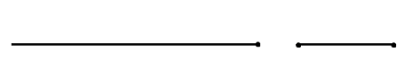
Fix an arbitrary point . Using rotation we can assume that , which will slightly simplify notation. Then define the line segments and , see Figure 1, and let be the family of all paths joining the sets and . Our intent is to estimate the values of and , and use the inequality (3.3) to obtain the desired upper bound for the winding of , which is the same as the winding in (3.2). Without loss of generality we can additionally assume that .
Let us first estimate from above when is small. To this end, construct balls , where goes trough numbers and is the smallest number for which . Then define
To see that is admissible for the path family note that every point belongs to some ball , we have when and for every . Using the mapping we estimate
| (3.4) |
To estimate this integral further we use the elementary inequality
which holds for any , to obtain the pointwise inequality
| (3.5) |
that holds almost everywhere. By combining (3.4) and (3.5) we obtain
| (3.6) |
As is a mapping with -exponentially integrable distortion and , the first integral is bounded from above by a constant . For the second integral we first note that
for small . For the rest of the integral we calculate
where was the smallest number for which , and thus . Hence by combining the above estimates with (3.6) we obtain
which gives
| (3.7) |
for all , for some .
Next we will estimate from below. Here we start with
and provide a lower bound for
| (3.8) |
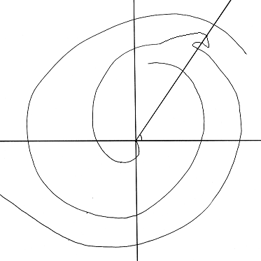
that holds for every direction and an arbitrary admissible . We will estimate the integral (3.8) from below by first finding disjoint line segments , for which one endpoint lies in and the other in , and then using admissibility of to estimate its integral over these line segments. The main idea is to note that the paths and must cycle around the origin alternately, see figure 2 for illustration.
To see this, assume that the argument of the path increases by when moves from to , where . As the mapping is a homeomorphism and the path must contain the origin and points with big moduli, since when , the path must intersect the line segment at least once, let say at the point , where . We can choose and such that there are no points from the paths and in the line segment . These line segments are the ones we are looking for, and as the path cycles around the origin times we can define
| (3.9) |
and find at least disjoint line segments with desired endpoints. Thus we obtain, for every direction , that
| (3.10) |
where
and for every line segment the end points are in different sets . As every line segment belongs to the path family we can estimate the integral over any line segment , using the reverse Hölder inequality and admissibility of , by
| (3.11) |
Combining this with (3.10) we obtain
| (3.12) |
To estimate this further we will use the following technical lemma.
Lemma 3.2.
Let and be given, and let be positive numbers such that . Then
| (3.13) |
Proof. Choose the numbers such that we can find , and , for which . By elementary calculations we see that replacing with will decrease the value of the sum (3.13). Thus, if we would know that the sum (3.13) attains its minimum we would be ready, as the numbers given by the condition , for every , would then have to give this minimum and can be calculated to satisfy the equality in (3.13).
To show that the sum does attain its minimum we define
and note that it is compact. Then define the mapping on the set by
Note that if for every the sum (3.13) is coupled with by the relation . Let be such that is finite. As is a fixed number there exists such that
if , for some . Hence for every such that for some , and thus it is enough to look for the minimum in the set
As the set is compact and is continuous in the set the mapping attains its minimum in and hence also the sum (3.13) attains minimum, which finishes the proof.
We return to proving our main theorem. We continue from (3.12) by estimating
| (3.14) |
where in the last inequality we have used Lemma 3.2. To estimate further from (3.14) we must bound from below. To this end, use Theorem B from [5], with the formulation of (2.5), on the modulus of continuity to get that
| (3.15) |
when is small. Hence the estimate (3.14) together with (3.15) gives
for an arbitrary direction and small . Thus we have for these points that
| (3.16) |
We now have the estimates (3.7) and (3.16) for the moduli and , when the point is small. Then we use the inequality (3.3) with these estimates to obtain
and see
Thus, due to the equality (3.9), we have that
when . And since is finite for any fixed branch of the argument this proves Theorem 3.1, and hence also its renormalization Theorem 1.1.
We will next show that Theorem 1.1 is sharp up to the constant by proving that, given arbitrary parameters and satisfying the condition (1.7), the mapping
| (3.17) |
has -exponentially integrable distortion and that we can choose the parameters and such that the rotation is close to the bound given by Theorem 1.1. First note, that it is enough to calculate the distortion function in the ball , as otherwise it is bounded by some constant. To do this compute the complex derivatives
| (3.18) |
and
| (3.19) |
Then calculate the modulus of the Beltrami coefficient
| (3.20) |
And finally use the equation with (3.20) to obtain
where is bounded, for , and as . Thus is -exponentially integrable when
From this we obtain that
| (3.21) |
and
where in the last inequality we use the bound (3.21) for . This shows that given an arbitrary we can choose the parameters and such that the mapping (3.17) satisfies
for all . Clearly the mappings are sense-preserving homeomorphisms. From the calculations (3.18) and (3.19), together with the definition (3.17), we see that they lie in the Sobolev space , and thus also have locally integrable Jacobian. Hence these mappings have finite distortion and thus prove that Theorem 1.1 is sharp up to the constant , and additionally that the rotation
can be attained.
Regarding the remarks on the relation between stretching and rotation we first calculate the distortion of the mappings (1.5), defined by
in a similar manner as for the mappings (3.17), and obtain that
where is bounded and as . This proves that has -exponentially integrable distortion when
and with a similar reasoning as for the mappings (3.17) we see that is a mapping of finite distortion. Moreover, since , we see that grows like as .
However, the pointwise stretching of does bound the pointwise rotation even in the case of mappings with exponentially integrable distortion, but the relation between stretching and rotation is different from the quasiconformal case. This follows from (3.15), where we use the modulus of continuity. If in (3.15) we would instead of
assume
| (3.22) |
where , and continue after (3.15) as in the proof of Theorem 3.1 we would obtain
| (3.23) |
where is a constant depending on the constant chosen in (3.22). This shows how stretching bounds rotation from above. To see that this relation between stretching and rotation is optimal, again up to the constant , we present the mappings
| (3.24) |
where and . These mappings can be checked to be mappings of finite distortion with -exponentially integrable distortion when
| (3.25) |
with a similar calculation as for the mappings (3.17). From (3.25) we see that can be arbitrary big if we choose sufficiently big , and hence the constant truly does depend on the stretching and there is no absolute constant for which (3.23) would hold.
References
- [1] K. Astala, T. Iwaniec, and G. J. Martin, Elliptic partial differential equations and quasiconformal mappings in the plane, Princeton University Press, 2009.
- [2] K. Astala, T. Iwaniec, I. Prause, and E. Saksman, Bilipschitz and quasiconformal rotation, stretching and multifractal spectra, Publ. Math. Inst. Hautes tudes Sci. June 2015, Volume 121, Issue 1, 113–154.
- [3] Z. Balogh, K. Fässler and I. Platis, Modulus of curve families and extremality of spiral-stretch maps, J. Anal. Math. 113 (2011), 265–291.
- [4] V. Gutlyanski and O. Martio, Rotation estimates and spirals, Conform. Geom. Dyn. 5 (2001), 6–20.
- [5] D. Herron and P. Koskela, Mappings of finite distortion: gauge dimension of generalized quasi-circles, Illinois J. Math. 47 (2003), 1243–1259.
- [6] F. John, Rotation and strain, Comm. Pure Appl. Math., 14 (1961), 391–413.
- [7] P. Koskela and J. Onninen, Mappings of finite distortion: capacity and modulus inequalities, J. Reine Angew. Math. 599 (2006), 1–26.
- [8] J. Onninen and X. Zhong, A note on mappings of finite distortion: the sharp modulus of continuity, Michigan Math. J. 53 (2005), no. 2, 329–335.
- [9] J. Väisälä, Lectures on -dimensional quasiconformal mappings, Lecture notes in math., 229, Springer-Verlag, Berlin-New York, 1972.