$T$-optimal discriminating designs for Fourier
regression models

In this paper we consider the problem of constructing $T$-optimal discriminating designs for Fourier regression models. We provide explicit solutions of the optimal design problem for discriminating between two Fourier regression models, which differ by at most three trigonometric functions. In general, the $T$-optimal discriminating design depends in a complicated way on the parameters of the larger model, and for special configurations of the parameters $T$-optimal discriminating designs can be found analytically. Moreover, we also study this dependence in the remaining cases by calculating the optimal designs numerically. In particular, it is demonstrated that $D$- and $D_{s}$-optimal designs have rather low efficiencies with respect to the $T$-optimality criterion.

Keywords and Phrases: $T$-optimal design; model discrimination; linear optimality criteria; Chebyshev polynomial, trigonometric models

AMS subject classification: 62K05

1 Introduction

The problem of identifying an appropriate regression model in a class of competing candidate models is one of the most important problems in applied regression analysis. Nowadays it is well known that a well designed experiment can improve the performance of model discrimination substantially, and several authors have addressed the problem of constructing optimal designs for this purpose. The literature on designs for model discrimination can roughly be divided into two parts. Hunter and Reiner, (1965), Stigler, (1971) considered two nested models, where the extended model reduces to the “smaller” model for a specific choice of a subset of the parameters. The optimal discriminating designs are then constructed such that these parameters are estimated most precisely. Since these fundamental papers several authors have investigated this approach in various regression models [see Hill, (1978), Studden, (1982), Spruill, (1990), Dette, (1994, 1995), Dette and Haller, (1998), Song and Wong, (1999), Zen and Tsai, (2004), Biedermann et al., (2009) among many others]. The second line of research was initialized in a fundamental paper of Atkinson and Fedorov, 1975a , who introduced the $T$-optimality criterion for discriminating between two competing regression models. Since the introduction of this criterion, the problem of determining $T$-optimal discriminating designs has been considered by numerous authors [see Atkinson and Fedorov, 1975b , Ucinski and Bogacka, (2005), Dette and Titoff, (2009), Atkinson, (2010), Tommasi and López-Fidalgo, (2010) or Wiens, (2009, 2010) among others]. The $T$-optimal design problem is essentially a minimax problem, and – except for very simple models – the corresponding optimal designs are not easy to find and have to be determined numerically in most cases of practical interest. On the other hand, analytical solutions are helpful for a better understanding of the optimization problem and can also be used to validate numerical procedures for the construction of optimal designs. Some explicit solutions of the $T$-optimal design problem for discriminating between two polynomial regression models can be found in Dette et al., (2012), but to our best knowledge no other analytical solutions are available in the literature.

In the present paper we consider the problem of constructing $T$-optimal discriminating designs for Fourier regression models, which are widely used to describe periodic phenomena [see for example Lestrel, (1997)]. Optimal designs for estimating all parameters of the Fourier regression model have been discussed by numerous authors [see e.g. Karlin and Studden, (1966), page 347, Lau and Studden, (1985), Kitsos et al., (1988), Riccomagno et al., (1997) and Dette and Melas, (2003) among others]. Discriminating design problems in the spirit of Hunter and Reiner, (1965), Stigler, (1971) have been discussed by Biedermann et al., (2009), Zen and Tsai, (2004) among others, but $T$-optimal designs for Fourier regression models, have not been investigated in the literature so far. In Section 2 we introduce the problem and provide a characterization of $T$-optimal discriminating designs in terms of a classical approximation problem. Explicit solutions of the $T$-optimal design problem for Fourier regression models are discussed in Section 3. Finally, in Section 4 we provide some numerical results of these challenging optimization problems. In particular, we demonstrate that the structure (more precisely the number of support points) of the $T$-optimal discriminating design depends sensitively on the location of the parameters.

2 $T$-optimal discriminating designs

Consider the classical regression model

$$y=\eta(x)+\varepsilon,$$ (2.1)

where the explanatory variable $x$ varies in a compact design space, say $\cal X$, and observations at different locations, say $x$ and $x^{\prime}$, are assumed to be independent. In (2.1) the quantity $\varepsilon$ denotes a random variable with mean 0 and variance $\sigma^{2}$, and $\eta(x)$ is a function, which is called regression function in the literature [see Seber and Wild, (1989)]. We assume that the experimenter has two parametric models, say $\eta_{1}(x,\theta_{1})$ and $\eta_{2}(x,\theta_{2})$, for this function in mind to describe the relation between predictor and response, and that the first goal of the experiment is to identify the appropriate model from these two candidates. In order to find “good” designs for discriminating between the models $\eta_{1}$ and $\eta_{2}$ we consider approximate designs in the sense of Kiefer, (1974), which are probability measures on the design space $\mathcal{X}$ with finite support. The support points, say $x_{1},\dots,x_{s}$, of an (approximate) design $\xi$ define the locations where observations are taken, while the weights denote the corresponding relative proportions of total observations to be taken at these points. If the design $\xi$ has masses $\omega_{i}>0$ at the different points $x_{i}\>(i=1,\dots,s)$ and $n$ observations can be made, the quantities $\omega_{i}n$ are rounded to integers, say $n_{i}$, satisfying $\sum^{s}_{i=1}n_{i}=n$, and the experimenter takes $n_{i}$ observations at each location $x_{i}\>(i=1,\dots,s)$ [see for example Pukelsheim and Rieder, (1992)].
For the construction of a good design for discriminating between the models $\eta_{1}$ and $\eta_{2}$ Atkinson and Fedorov, 1975a proposed in a seminal paper to fix one model, say $\eta_{2}$, and to determine the discriminating design such that the minimal deviation between the model $\eta_{2}$ and the class of models defined by $\eta_{1}$ is maximized. More precisely, a $T$-optimal design is defined $\xi^{*}$ by

$$\xi^{*}=\arg\max_{\xi}\int_{\chi}\left(\eta_{2}(x,\theta_{2})-\eta_{1}(x,\widehat{\theta}_{1})\right)^{2}\xi(dx),$$

where the parameter $\widehat{\theta}_{1}$ minimizes the expression

$$\widehat{\theta}_{1}=\arg\min_{\theta_{1}}\int_{\chi}\left(\eta_{2}(x,\theta_{2})-\eta_{1}(x,\theta_{1})\right)^{2}\xi(dx).$$

Note that the $T$-optimality criterion is a local optimality criterion in the sense of Chernoff, (1953), because it requires knowledge of the parameter $\theta_{2}$. Bayesian versions of this criterion have recently been investigated by Dette et al., (2013) and Dette et al., 2015a .

In the present work we consider cases, where the competing regression functions are given by two Fourier regression models of different order, that is

$$\eta_{1}(x,\theta_{1})=\overline{q}_{0}+\sum_{i=1}^{k_{1}}\overline{q}_{2i-1}\sin(ix)+\sum_{i=1}^{k_{2}}\overline{q}_{2i}\cos(ix)$$ (2.2)

and

$$\eta_{2}(x,\theta_{2}) = \tilde{q}_{0}+\sum_{i=1}^{k_{1}}\tilde{q}_{2i-1}\sin(ix)+\sum_{i=1}^{k_{2}}\tilde{q}_{2i}\cos(ix)$$

$$+ \sum_{i=k_{1}+1}^{m}b_{2(i-k_{1})-1}\sin(ix)+\sum_{i=k_{2}+1}^{m}b_{2(i-k_{2})}\cos(ix),$$

where

$$\theta_{1} = (\overline{q}_{0},\overline{q}_{2},\ldots,\overline{q}_{2k_{2}},\overline{q}_{1},\ldots,\overline{q}_{2k_{1}-1})$$

$$\theta_{2} = (\tilde{q}_{0},\ldots,\tilde{q}_{2k_{2}},\tilde{q}_{1},\ldots,\tilde{q}_{2k-1},b_{2},\ldots,b_{2m},b_{1},\ldots,b_{2m-1})$$

are the parameter vectors in model $\eta_{1}$ and $\eta_{2}$, respectively. Fourier regression models are widely used to describe periodic phenomena [see e.g. Mardia, (1972), or Lestrel, (1997)] and the problem of designing experiments for Fourier regression models has been discussed by several authors [see the cited references in the introduction]. However, the problem of constructing $T$-optimal discriminating designs for these models has not been addressed in the literature so far.

We assume that the design space is given by the interval $\chi=[0,2\pi]$ and denote the difference $\eta_{2}(x,\theta_{2})-\eta_{1}(x,\theta_{1})$ by

$$\overline{\eta}(x,q,\overline{b}) = q_{0}+\sum_{i=1}^{k_{1}}q_{2i-1}\sin(ix)+\sum_{i=1}^{k_{2}}q_{2i}\cos(ix)$$

$$+\sum_{i=k_{1}+1}^{m}b_{2(i-k_{1})-1}\sin(ix)+\sum_{i=k_{2}+1}^{m}b_{2(i-k_{2})}\cos(ix),$$

where $q=(q_{0},q_{1},\ldots,q_{2k_{1}-1},q_{2},\ldots,q_{2k_{2}})$, $q_{i}=\tilde{q}_{i}-\overline{q}_{i}$ and $\overline{b}=(b_{1},b_{3},\ldots,b_{2(m-k_{1})-1},b_{2},b_{4},\ldots,b_{2(m-k_{2})})^{T}$ denotes the vector of “additional” parameters in model (2). With these notations the $T$-optimality criterion reduces to

$$T(\xi,\overline{b})=\min_{q}\int^{2\pi}_{0}\overline{\eta}^{2}(x,q,\overline{b})\xi(dx),$$

and a $T$-optimal design for discriminating between the models (2.2) and (2) maximizes $T(\xi,\overline{b})$, that is

$$\xi^{*}=\arg\max_{\xi}T(\xi,\overline{b}).$$

The following result provides a characterization of $T$-optimal designs and is known in the literature as the equivalence theorem for $T$-optimality [see, for instance, Theorem 2.2 in Dette and Titoff, (2009)].

Theorem 2.1

For a fixed vector $\overline{b}$ the following conditions are equivalent:

• The design

  $$\xi^{*}=\left(\begin{array}[]{ccc}x^{*}_{1}&\ldots&x^{*}_{n}\\ \omega_{1}&\ldots&\omega_{n}\end{array}\right),\,\,x_{i}\in[0,2\pi],\,\,i=1,\ldots,n.$$

  is a $T$-optimal for discriminating designs for the models $\eta_{1}$ and $\eta_{2}$.

• There exists a vector $\theta^{*}$ and a positive constant $h$ such, that the function $\psi^{*}(x)=\overline{\eta}(x,\theta^{*},\overline{b})$ satisfies the following conditions

  • $|\psi^{*}(x)|\leq h$,  for all  $x\in[0,2\pi]$,

  • $|\psi^{*}(x_{i})|=h$,  for all  $i=1,2,\dots,n$.

  • The support points $x^{*}_{i}$ and weights $\omega_{i}$ of the design $\xi^{*}$ satisfy the conditions

    $$\sum^{n}_{i=1}\psi^{*}(x^{*}_{i})\frac{\partial\overline{\eta}(x^{*}_{i},\theta,\overline{b})}{{\displaystyle\partial\theta_{j}}}\omega_{i}\Big{|}_{\theta=\theta^{*}}=0,\quad j=0,\ldots,k_{1}+k_{2}.$$ (2.6)

Note that Theorem 2.1 is not restricted to Fourier regression models but holds in general for linear models. A detailed discussion can be found in Dette and Titoff, (2009). As pointed out in the introduction, the explicit determination of $T$-optimal discriminating designs is a very challenging problem. The complexity of the problem depends on the dimension of the vector $\overline{b}$. In the following Sections 3 and 4 we provide explicit and numerical solutions of this difficult optimal design problem for Fourier regression models. In particular, we will demonstrate that the structure of the $T$-discriminating design (such as the number of support points) depends on the location of the vector $\overline{b}$ in the $(2m-k_{1}-k_{2})$-dimensional Euclidean space.

3 Explicit solutions

In this section we give some explicit $T$-optimal discriminating designs for Fourier regression models. In particular we consider the problem of constructing $T$-optimal discriminating designs for the models (2.2) and (2), where

$$k_{1}=k_{2}=m-1,$$ (3.1)

$$k_{1}=m-1,\ k_{2}=m-2,$$ (3.2)

$$k_{1}=m-2,\ k_{2}=m-1.$$ (3.3)

We give an explicit solution for the case (3.1), while for the case (3.2) explicit results are provided in Section 3.2 for specific values of the parameters $b_{\ell}$ in model (2). Corresponding results for the case (3.3) are briefly mentioned in Remark 3.1. In general the solution of the $T$-optimal design problem depends in a complicated way on the parameters $\overline{b}$, and we demonstrate numerically in Section 4 that the number of support points of the $T$-optimal discriminating design changes if the vector $\overline{b}$ is located in different areas of the space $\mathbb{R}^{2}$.

3.1 Discriminating designs for $k_{1}=k_{2}=m-1$

Throughout this section we assume that $k_{1}=k_{2}=m-1$ and rewrite the function in (2) as

$$\overline{\eta}(x,q,\overline{b})=q_{0}+\sum_{i=1}^{m-1}q_{2i-1}\sin(ix)+\sum_{i=1}^{m-1}q_{2i}\cos(ix)+b_{1}\sin(mx)+b_{2}\cos(mx).$$

Our first result gives an explicit solution of the $T$-optimal design problem in the case $b_{1},b_{2}\neq 0$.

Theorem 3.1

Consider the Fourier regression models (2.2) and (2) with $k_{1}=k_{2}=m-1$. Let $b_{1},b_{2}\neq 0$, then the design

$$\xi^{*}=\begin{pmatrix}\frac{1}{m}\arctan(\frac{1}{b})&\frac{1}{m}\arctan(\frac{1}{b})+\frac{\pi}{m}&\dots&\frac{1}{m}\arctan(\frac{1}{b})+\frac{(2m-1)\pi}{m}\\ \frac{1}{2m}&\frac{1}{2m}&\dots&\frac{1}{2m}\end{pmatrix}$$ (3.4)

is a $T$-optimal discriminating design, where $b=b_{2}/b_{1}$.

Proof. We consider the function

$$\psi^{*}(x)=\overline{\eta}(x,0,\overline{b})=b_{1}\sin(mx)+b_{2}\cos(mx)$$

and prove that this function and the weights $\omega^{*}_{i}=\frac{1}{2m}$ and support points $x_{i}^{*}=\frac{1}{m}\arctan(\frac{1}{b})+\frac{(i-1)}{m}\pi$ of the design $\xi^{*}$ defined in (3.4) satisfy the conditions of Theorem 2.1.

Direct calculations show for the support points of the design $\xi^{*}$ the identities

$$\psi^{*}(x^{*}_{i})=(-1)^{i-1}\sqrt{b^{2}_{1}+b^{2}_{2}},\qquad i=1,\ldots,2m.$$

Consequently, the function $\psi^{*}$ satisfies conditions (i)-(ii) for $h=\sqrt{b^{2}_{1}+b^{2}_{2}}$, and it remains to show that the equations in (2.6) hold. In other words, we have to check that the equalities

$$\sum^{n}_{i=1}(-1)^{i}\sin(jx_{i}^{*})=0,\ \ \sum^{n}_{i=1}(-1)^{i}\cos(jx_{i}^{*})=0,\ \ j=0,\ldots,m-1,$$ (3.5)

are satisfied. Observing the identities $\sin(\alpha+\beta)=\sin(\alpha)\cos(\beta)+\cos(\alpha)\sin(\beta)$ and $\cos(\alpha+\beta)=\cos(\alpha)\cos(\beta)-\sin(\alpha)\sin(\beta)$ we can rewrite (3.5) as

$$\sum^{2m}_{i=1}(-1)^{i}\sin\Big{(}j\frac{(i-1)\pi}{m}\Big{)}=0,\ \ \sum^{2m}_{i=1}(-1)^{i}\cos\Big{(}j\frac{(i-1)\pi}{m}\Big{)}=0,\ \ j=0,\ldots,m-1.$$

These equalities are a consequence of the identity

$$\sum^{2m-1}_{\ell=0}e^{\frac{i\pi\ell j}{m}}(-1)^{\ell}=0\qquad j=1,\ldots,m-1$$

(here $i=\sqrt{-1}$ and the case $j=0$ has to be considered separately), and the assertion of Theorem 3.1 now follows from Theorem 2.1. $\Box$

Corollary 3.1

Consider the Fourier regression models (2.2) and (2) with $k_{1}=k_{2}=m-1$. If $b_{1}=0$, then the design

$$\xi^{*}=\begin{pmatrix}0&\frac{\pi}{m}&\dots&\frac{(2m-1)\pi}{m}\\ \frac{1}{2m}&\frac{1}{2m}&\dots&\frac{1}{2m}\end{pmatrix}$$

is a $T$-optimal discriminating design. If $b_{2}=0$, then the design

$$\xi^{*}=\begin{pmatrix}\frac{\pi}{2m}&\frac{3\pi}{2m}&\dots&\frac{(4m-1)\pi}{2m}\\ \frac{1}{2m}&\frac{1}{2m}&\dots&\frac{1}{2m}\end{pmatrix}$$

is a $T$-optimal discriminating design.

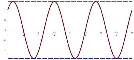
Figure 1: The function $\psi^{*}$ of Theorem 2.1 for the two Fourier regression models (3.6) and (3.7) ($b_{1}=b_{2}=1$).

Example 3.1

Suppose that $m=3,$ $b_{1}=b_{2}=1$ and $k_{1}$=$k_{2}$=2, then if follows from Theorem 3.1 that the design with equal masses at the six points $\frac{1}{12}\pi$, $\frac{5}{12}\pi$, $\frac{3}{4}\pi$, $\frac{13}{12}\pi$, $\frac{17}{12}\pi$ and $\frac{7}{4}\pi$ is a $T$-optimal discriminating design for the two Fourier regression models

$$\overline{q}_{0}+\overline{q}_{1}\sin x+\overline{q}_{2}\cos x+\overline{q}_{3}\sin(2x)+\overline{q}_{4}\cos(2x)$$ (3.6)

$$\overline{q_{0}}+\tilde{q}_{1}\sin x+\tilde{q}_{2}\cos x+\tilde{q}_{3}\sin(2x)+\tilde{q}_{4}\cos(2x)+{b_{1}}\sin(3x)+{b_{2}}\cos(3x).$$ (3.7)

The function $\psi^{*}$ of Theorem 2.1 for this design is depicted in Figure 1.

3.2 Discriminating designs for $k_{1}=m-1,k_{2}=m-2$

Throughout this section we determine $T$-optimal discriminating designs for the trigonometric regression models

$$\eta_{1}(x,\theta_{1})= = \overline{q}_{0}+\sum^{m-1}_{i=1}\overline{q}_{2i-1}\sin(ix)+\sum^{m-2}_{i=1}\overline{q}_{2i}\cos(ix)$$ (3.8)

$$\eta_{2}(x,\theta_{2}) = \tilde{q}_{0}+\sum^{m-1}_{i=1}\tilde{q}_{2i-1}\sin(ix)+\sum^{m-2}_{i=1}\tilde{q}_{2i}\cos(ix)$$

$$+ b_{0}\cos((m-1)x)+b_{1}\sin(mx)+b_{2}\cos(mx).$$

Note that the two regression models in (2.2) and (2) now differ by three functions, that is $k_{1}=m-1,k_{2}=m-2$. In general, $T$-optimal discriminating designs for this case have to be determined numerically, and we will provide numerical results for $m=2$ and $m=3$ in the following Section 4. However, for some special configurations of the parameters, the $T$-optimal discriminating designs can also be found explicitly, and these cases will be discussed in the present section.

If $k_{1}=m-1,k_{2}=m-2$ the function $\overline{\eta}$ in (2) has the representation

$$\overline{\eta}(x,q,\overline{b})=q_{0}+\sum_{i=1}^{m-1}q_{2i-1}\sin(ix)+\sum_{i=1}^{m-2}q_{2i}\cos(ix)+b_{0}\cos((m-1)x)+b_{1}\sin(mx)+b_{2}\cos(mx).$$

We may assume without loss of generality that $b_{0}=1$. Indeed, if $b_{0}=0$, the optimal designs can be obtained from Theorem 3.1. Moreover, if $b_{0}\neq 0$, the $T$-optimal discriminating design does not depend on the particular value of $b_{0}$, since we can divide all coefficients by this parameter. After normalizing we therefore obtain

$$\overline{\eta}(x,q,\overline{b}) = q_{0}+\sum_{i=1}^{m-1}q_{2i-1}\sin(ix)+\sum_{i=1}^{m-2}q_{2i}\cos(ix)+\cos((m-1)x)$$

$$+b_{1}\sin(mx)+b_{2}\cos(mx).$$

We now concentrate on two special cases: $b_{1}=0,\ b_{2}\neq 0$ and $b_{2}=0,\ b_{1}\neq 0$, for which we can provide an explicit solution of the $T$-optimal design problem if the absolute value of the non-vanishing parameter is sufficiently large. For this purpose we define support points and weights as follows

$$x^{*}_{i}(b)=\arccos\Big{(}-\Big{(}1+\frac{1}{2m|b|}\Big{)}\cos\Big{(}\frac{(m-i+1)\pi}{m}\Big{)}-\frac{1}{2m|b|}\Big{)},\$$ (3.11)

$${\omega^{*}_{i}=\frac{1}{m}\cos^{2}\Big{(}\frac{(i-1)\pi}{2m}\Big{)},\ i=1,\ldots,m.\hskip 96.0002pt}$$ (3.12)

Our next result gives an explicit solution of the $T$-optimal design problem in the case $b_{1}=0,\ b_{2}\neq 0$.

Theorem 3.2

Consider the Fourier regression models (3.8) and (3.2) with $b_{0}=1$, $b_{1}=0$, $b_{2}\neq 0$.

• If $b_{2}>0$, $|b_{2}|\geq\frac{1}{2m}\cot^{2}\left(\frac{\pi}{2m}\right)$, then the design

  $$\xi^{*}_{1}=\left(\begin{array}[]{cccccc}x^{*}_{1}(b_{2})&\ldots&x^{*}_{m}(b_{2})&2\pi-x^{*}_{m}(b_{2})&\ldots&2\pi-x^{*}_{2}(b_{2})\\ \omega^{*}_{1}&\ldots&\omega^{*}_{m}&\omega^{*}_{m}&\ldots&\omega^{*}_{2}\end{array}\right)$$ (3.15)

  is a $T$-optimal discriminating design, where the support points and weights are defined in (3.11) and (3.12), respectively.

• If $b_{2}<0$, $|b_{2}|\geq\frac{1}{2m}\cot^{2}\left(\frac{\pi}{2m}\right)$, then the design

  $$\xi^{*}_{2}=\left(\begin{array}[]{cccccc}\pi-x^{*}_{m}(b_{2})&\ldots&\pi-x^{*}_{1}(b_{2})&\pi+x^{*}_{2}(b_{2})&\ldots&\pi+x^{*}_{m}(b_{2})\\ \omega^{*}_{m}&\ldots&\omega^{*}_{1}&\omega^{*}_{2}&\ldots&\omega^{*}_{m}\end{array}\right),$$ (3.18)

  is a $T$-optimal discriminating design, where the support points and weights are defined in (3.11) and (3.12), respectively.

Proof. We only consider the case $b_{2}\geq\frac{1}{2m}\cot^{2}(\frac{\pi}{2m})>0$ and note that the other case follows by similar arguments. We will use Theorem 2.1 and prove the existence of a vector $\theta^{*}$, such that the function $\psi^{*}(x)=\overline{\eta}(x,\theta^{*},\overline{b})$ satisfies conditions (i) - (iii) in this theorem. For this purpose let $T_{m}(x)=\cos(m\arccos x)$ denote the $m$th Chebyshev polynomial of the first kind, then it is follows by a straightforward calculation that there exists a vector $\theta^{*}$ such that the function

$$\psi^{*}(x)=\overline{\eta}(x,\theta^{*},\overline{b})=(-1)^{m}|b_{2}|\Big{(}1+\frac{1}{2m|b_{2}|}\Big{)}^{m}T_{m}\Big{(}\frac{-\cos(x)-\frac{1}{2m|b_{2}|}}{1+\frac{1}{2m|b_{2}|}}\Big{)},$$

is a trigonometric polynomial of degree $m$ with leading term $|b_{2}|\cos(mx)$ [note that the leading term of $T_{m}(x)$ is given by $2^{m-1}x^{m}$ and that $2^{m-1}(\cos x)^{m}=\cos(mx)+m\cos((m-2)x)+\ldots$]. Direct calculations show that the points $x^{*}_{i}(b_{2})$ defined in (3.11) are the extremal points of this function, that is

$$\psi^{*}(x^{*}_{i}(b_{2}))=(-1)^{i-1}|b_{2}|\Big{(}1+\frac{1}{2m|b_{2}|}\Big{)}^{m}\leavevmode\nobreak\ ,\qquad i=1,\ldots,m.$$ (3.19)

Consequently, $\psi^{*}$ satisfies conditions (i) and (ii) of Theorem 2.1. Finally, we prove the third condition (2.6). The corresponding equalities reduce to

$${\displaystyle\sum^{m}_{i=1}\omega^{*}_{i}\psi^{*}(x^{*}_{i}(b_{2}))\cos(jx^{*}_{i}(b_{2}))}+{\displaystyle\sum^{m}_{i=2}\omega^{*}_{i}\psi^{*}(2\pi-x^{*}_{i}(b_{2}))\cos\big{(}j(2\pi-x^{*}_{i}(b_{2}))\big{)}=0}$$ (3.20)

$(j=0,\ldots,m-2)$, and

$${\displaystyle\sum^{m}_{i=1}\omega^{*}_{i}\psi^{*}(x^{*}_{i}(b_{2}))\sin(jx^{*}_{i}(b_{2}))}+{\displaystyle\sum^{m}_{i=2}\omega^{*}_{i}\psi^{*}(2\pi-x^{*}_{i}(b_{2}))\sin\big{(}j(2\pi-x^{*}_{i}(b_{2})\big{)}=0}$$ (3.21)

$(j=1,\ldots,m-1)$. Observing (3.19), $x^{*}_{1}(b_{2})=0$ and the identity $\psi^{*}(x)=\psi^{*}(2\pi-x)$ we can rewrite the left hand side of (3.21) as

$$\sum^{m}_{i=2}\omega^{*}_{i}\big{(}\sin(jx^{*}_{i}(b_{2}))+\sin(j(2\pi-x_{i}^{*}(b_{2})))\big{)}=\sum^{m}_{i=2}\omega^{*}_{i}\big{(}\sin(jx^{*}_{i}(b_{2}))-\sin(jx^{*}_{i}(b_{2}))\big{)}$$

$(j=1,\ldots,m-1)$. Consequently (3.21) is obviously satisfied. Similarly, we obtain for (3.20)

$$\sum^{m}_{i=1}\overline{\omega}_{i}(-1)^{i}\cos(jx^{*}_{i}(b_{2}))=0,\ \ j=0,\ldots,m-2,\$$ (3.22)

where we use the notations $\overline{\omega}_{1}=\frac{\omega^{*}_{1}}{2}$, $\overline{\omega}_{i}=\omega^{*}_{i},\ i=0,\ldots,m-2$ in (3.22). Defining $t_{i}=\cos(x^{*}_{i}(b_{2}))$ we obtain for the left hand side of (3.22)

$$\sum^{m}_{i=1}\overline{\omega}_{i}(-1)^{i}\cos(jx^{*}_{i}(b_{2}))=\sum^{m}_{i=1}\sum^{m-2}_{p=0}\overline{\omega}_{i}(-1)^{i}a_{p}t_{i}^{p}=\sum^{m-2}_{p=0}a_{p}\sum^{m}_{i=1}\overline{\omega}_{i}(-1)^{i}t_{i}^{p}$$

for some coefficients $a_{p}$. It is proved in Appendix A.1 of Dette et al., (2012) that

$$\sum^{m}_{i=1}\overline{\omega}_{i}(-1)^{i}t_{i}^{p}=0,\leavevmode\nobreak\ \leavevmode\nobreak\ p=0,\ldots,m-2$$

which implies (3.20). The $T$-optimality of the design $\xi^{*}_{1}$ now directly follows from Theorem 2.1. $\Box$

The next theorem considers the case $b_{1}\neq 0,\ b_{2}=0$, which is substantially harder. Here we are able to determine the $T$-optimal discriminating designs explicitly if the degree $m$ of the Fourier regression model is odd.

Theorem 3.3

Consider the Fourier regression models (3.8) and (3.2) with $b_{0}=1,b_{1}\neq 0,b_{2}=0$, where $m$ is odd. For $\ell=1,2$ let $t^{(\xi_{\ell})}_{i}$ and $\omega^{(\xi_{\ell})}_{i}$, denote the support points and weights of the designs $\xi^{*}_{1}$ and $\xi^{*}_{2}$ defined in (3.15) and (3.18) and define

$$t^{(\ell)}_{i}=t^{(\xi_{\ell})}_{i}+\frac{\pi}{2}\ mod\ 2\pi;\leavevmode\nobreak\ \leavevmode\nobreak\ \ell=1,2.$$

• If $b_{1}\geq\frac{1}{2m}\cot^{2}\left(\frac{\pi}{2m}\right)$, then the design

  $$\widetilde{\xi}^{*}_{1}=\left(\begin{array}[]{ccc}t^{(1)}_{1}&\ldots&t^{(1)}_{2m-1}\\ \omega^{(\xi_{1})}_{1}&\ldots&\omega^{(\xi_{1})}_{2m-1}\end{array}\right)$$ (3.25)

  is a $T$-optimal discriminating design.

• If $b_{1}<0$, $|b_{1}|\geq\frac{1}{2m}\cot^{2}\left(\frac{\pi}{2m}\right)$, then the design

  $$\widetilde{\xi}^{*}_{2}=\left(\begin{array}[]{ccc}t^{(2)}_{1}&\ldots&t^{(2)}_{2m-1}\\ \omega^{(\xi_{2})}_{1}&\ldots&\omega^{(\xi_{2})}_{2m-1}\end{array}\right)$$ (3.28)

  is a $T$-optimal discriminating design.

Proof. The proof is similar to the proof of Theorem 3.2, where we use the function

$$\psi^{*}(x)=\overline{\eta}(x,\theta^{*},\overline{b})=(-1)^{\frac{m+1}{2}}|b_{1}|\Big{(}1+\frac{1}{2m|b_{1}|}\Big{)}^{m}T_{m}\Big{(}\frac{-\sin(x)-\frac{1}{2m|b_{1}|}}{1+\frac{1}{2m|b_{1}|}}\Big{)},$$

in Theorem 2.1 The fact that this function is of the form

$$q_{0}+\sum^{2d-2}_{i=1}q_{2i-1}\sin(ix)+\sum^{2d-3}_{i=1}q_{2i}\cos(ix)+\cos((2d-2)x)+b_{1}\sin((2d-1)x)$$

and satisfies the assumptions of Theorem 2.1 follows from the identity

$$\cos\big{(}(2d-1)\arccos(t)\big{)}\equiv(-1)^{d-1}\sin\big{(}(2d-1)\arcsin(t)\big{)},\ t\in[-1,1],\ d=1,2,\ldots,$$ (3.29)

which can be used in the case $m=2d-1$. The details are omitted for the sake of brevity. $\Box$

Example 3.2

Consider the case $m=5$, $b_{1}=0$, $b_{2}=2$ and $k_{1}=4$, $k_{2}=3$. The $T$-optimal discriminating design can be obtained from Theorem 3.2 and is given by

$$\xi_{1}^{*}=\begin{pmatrix}0&0.65&1.29&1.95&2.69&3.59&4.33&4.99&5.64\\ 0.20&0.18&0.13&0.07&0.02&0.02&0.07&0.13&0.18\end{pmatrix}$$

Similarly, if $b_{1}=2,b_{2}=0$ the $T$-optimal discriminating design is given by

$$\tilde{\xi}_{1}^{*}=\begin{pmatrix}1.57&2.21&2.86&3.52&4.26&5.16&5.9&0.28&0.93\\ 0.20&0.18&0.13&0.07&0.02&0.02&0.07&0.13&0.18\end{pmatrix}$$

Note that the design $\tilde{\xi}^{*}_{1}$ is obtained from the design $\xi^{*}_{1}$ by the transformation $x\to x+\frac{\pi}{2}$. In Figure 2 we display the function $\psi^{*}$ in the equivalence Theorem 2.1 for both cases.

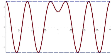
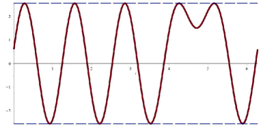
Figure 2: The function $\psi^{*}$ of Theorem 2.1 for two Fourier regression models of the form (3.8) and (3.2) with $m=5$. Left part: design $\xi_{1}^{*}$ of Theorem 3.2 ($b_{0}=1$, $b_{1}=0$, $b_{2}=2$), right part: design $\widetilde{\xi}^{*}_{1}$ of Theorem 3.3 ($b_{0}=1$, $b_{1}=2$, $b_{2}=0$).

Remark 3.1

In the case $k_{1}=m-2,k_{2}=m-1$ explicit solutions can be obtained by similar arguments as given in the proof of Theorem 3.2 and 3.3. If $m=2d$ is even and $b_{1}=0$ the function $\overline{\eta}$ is given by

$$\overline{\eta}(x,q,\overline{b})=q_{0}+\sum_{i=1}^{2d-2}q_{2i-1}\sin(ix)+\sum_{i=1}^{2d-1}q_{2i}\cos(ix)+\sin((2d-1)x)+b_{2}\cos(2dx)\leavevmode\nobreak\ .$$ (3.30)

If $b_{2}\geq\frac{1}{2m}\cot(\frac{\pi}{2m})$, the $T$-optimal discriminating design for the Fourier regression models (2.2) and (2) with $k_{1}=m-2$ and $k_{2}=m-1$ is given by the design (3.25), where the support points and weights are defined by

$$t^{(1)}_{i} = t^{(\xi_{1})}_{i}+\frac{3\pi}{2}\ \mod\ 2\pi;\leavevmode\nobreak\ \leavevmode\nobreak\ i=1,2,\ldots,2m-1\leavevmode\nobreak\ ,$$

$$\omega^{(1)}_{i} = \omega^{(\xi_{1})}_{i};\leavevmode\nobreak\ \leavevmode\nobreak\ i=1,2,\ldots,2m-1\leavevmode\nobreak\ ,$$

respectively, and $t^{(\xi_{1})}_{i}$ and $\omega^{(\xi_{1})}_{i};$ are the support points of the design $\xi_{1}^{*}$ in (3.15). The extremal polynomial $\psi^{*}$ in Theorem 2.1 is given by

$$\psi^{*}(x)=\overline{\eta}(x,\theta^{*},\overline{b})=(-1)^{\frac{m}{2}}|b_{1}|\Big{(}1+\frac{1}{2m|b_{1}|}\Big{)}^{m}T_{m}\Big{(}\frac{-\sin(x)+\frac{1}{2m|b_{1}|}}{1+\frac{1}{2m|b_{1}|}}\Big{)},$$

where the fact that $\psi^{*}$ can be represented in the form (3.30) follows from (3.29). A similar result is available in the case $b_{2}<0,|b_{2}|\geq\frac{1}{2m}\cot(\frac{\pi}{2m})$ and the details are omitted for the sake of brevity.

4 Some numerical results

The results of Section 3.2 are only correct if the module of $b_{1}$ or $b_{2}$ is larger or equal to some threshold. Otherwise $T$-optimal designs have a more complicated structure and have to be found numerically [see Dette et al., 2015b for some algorithms]. In this section we provide some more insight in the structure of $T$-optimal discriminating designs in cases, where an analytical determination of the optimal design is not possible. For this purpose we consider the Fourier regression models (3.8) and (3.2), where $b_{0}=1$ and $b_{1},\ b_{2}\neq 0$. Recalling the representation (3.2) for the function $\overline{\eta}$ in (2), we see that the support points and weights of the optimal $T$-discriminating designs depend on the two parameters $b_{1},b_{2}$ of the extended model. Moreover, the structure of the optimal design changes and depends on the location of the point ($b_{1},b_{2}$). We have calculated $T$-optimal discriminating designs for the Fourier regression models (3.8) and (3.2) for $m=2$ and $m=3$.

If $m=2$ the $T$-optimal designs have either $2$ or $3$ support points, and the corresponding areas for the point $(b_{1},b_{2})$ are depicted in the left part of Figure 3. For example, if $b_{1}=0$ and $|b_{2}|\geq 0.25$ the locally $T$-optimal discriminating design has $3$ support points (which coincides with the results of Theorem 3.2), while in the opposite case the optimal design is supported at only two points. This pattern does not change if $b_{1}\not=0$, but the threshold is slightly increasing. Numerical calculations show that the threshold converges to $\frac{\sqrt{2}}{4}$ as $b_{1}\to\infty$.

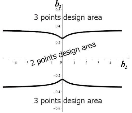
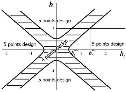
Figure 3: The number of support points of the $T$-optimal design for the Fourier regression models (3.8) and (3.2). Left part: $m=2$, right part: $m=3$.

The right part of Figure 3 shows corresponding results for the case $m=3$, and we see that the plane is separated into five parts. Four of them correspond to parameter configurations, where the $T$-optimal discriminating design is supported at $5$ points. Additionally, there exists one component, where a $4$-point design is $T$-optimal for discriminating between the two Fourier regression models. Consider for example the situation, where $b_{2}=1$ and $b_{1}$ varies in the interval $[0,3]$. In this case there exist two values, say $b_{1}^{min}$ and $b_{1}^{max}$, where the line through the point $(0,1)$ in the direction $(1,0)$ intersects the boundary of the fourth region [see the right part of Figure 3]. If $b_{1}\in[0,b_{1}^{min}]$ the $T$-optimal discriminating design has $5$ support points, while it has only $4$ support points if $b_{1}\in[b_{1}^{min},b_{1}^{max}]$. Finally, on the interval $[b_{1}^{max},3]$ the $T$-optimal discriminating design has again $5$ support points. The support points and corresponding weights of the $T$-optimal discriminating design are shown in Figure 4 [for the Fourier regression models (3.8) and (3.2)] as a function of the parameter $b_{1}\in[0,3]$ where $b_{2}=1$.

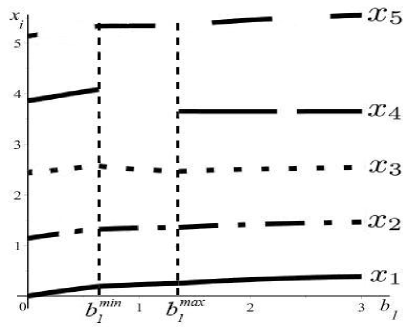
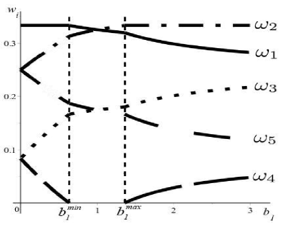
Figure 4: The support points and weights of the $T$-optimal discriminating design for the Fourier regression models (3.8) and (3.2), where $m=3$, $b_{0}=1$, $b_{2}=1$, and $b_{1}\in[0,3]$.

We conclude this section investigating the $T$-efficiency

$$\mbox{Eff}_{T}(\xi,b)=\frac{T(\xi,b)}{\max_{\eta}T(\eta,b)}$$

of some commonly used designs in this context. The first design is the $D$-optimal design for the extended model (2). The design can be found in Pukelsheim, (2006) and is given by

$$\xi_{D}^{*}=\begin{pmatrix}0&\frac{\pi}{4}&\frac{\pi}{2}&\frac{3\pi}{4}&\pi&\frac{5\pi}{4}&\frac{3\pi}{2}&\frac{7\pi}{4}\\ &&&&&&\\ \frac{1}{8}&\frac{1}{8}&\frac{1}{8}&\frac{1}{8}&\frac{1}{8}&\frac{1}{8}&\frac{1}{8}&\frac{1}{8}\end{pmatrix}$$

The second design is a discriminating design in the sense of Stigler, (1971). This design provides a most accurate estimation of the three highest coefficients $b_{0},b_{1}$ and $b_{2}$ in model (3.2) and can be obtained from the results of Lau and Studden, (1985). The design is given by

$$\xi^{*}_{D_{3}}=\begin{pmatrix}0&\frac{\pi}{4}&\frac{\pi}{2}&\frac{3\pi}{4}&\pi&\frac{5\pi}{4}&\frac{3\pi}{2}&\frac{7\pi}{4}\\ &&&&&&\\ \frac{3}{20}&\frac{1}{10}&\frac{3}{20}&\frac{1}{10}&\frac{3}{20}&\frac{1}{10}&\frac{3}{20}&\frac{1}{10}\end{pmatrix}$$

and will be called $D_{3}$-optimal design throughout this section. The corresponding efficiencies are shown in Figure 5 for various values of $b_{2}$, where the parameter $b_{1}$ varies in the interval $[0,5]$.

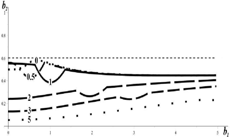
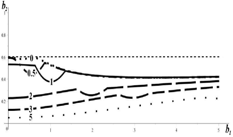
Figure 5: The $T$-efficiency of the $D$-optimal design (left part) and $D_{3}$-optimal design (right part) for discriminating between the Fourier regression models (3.8) and (3.2), where $m=3$, $b_{2}=0,0.5,1,2,3,5$, $b_{1}\in[0,5]$.

Both designs have rather similar $T$-efficiencies which are always smaller than $60\%$. This similarity can be explained by the fact that the $D$- and $D_{3}$-optimal design have the same support and only differ with respect to their weights. The efficiencies are decreasing with the parameter $b_{2}$. For larger values of $b_{2}$ the efficiencies of the $D$-and $D_{3}$-optimal design are very low. For fixed $b_{2}$ and larger values of $b_{1}$ the efficiencies do not change substantially.

Acknowledgements The authors would like to thank Martina Stein, who typed parts of this manuscript with considerable technical expertise. The work of V.B. Melas and P. Shpilev was supported by St. Petersburg State University (project "Actual problems of design and analysis for regression models", 6.38.435.2015). This work has also been supported in part by the Collaborative Research Center “Statistical modeling of nonlinear dynamic processes” (SFB 823, Teilprojekt C2) of the German Research Foundation (DFG) and by a grant from the National Institute Of General Medical Sciences of the National Institutes of Health under Award Number R01GM107639. The content is solely the responsibility of the authors and does not necessarily represent the official views of the National Institutes of Health.

References

- Atkinson, (2010) Atkinson, A. C. (2010). The non-uniqueness of some designs for discriminating between two polynomial models in one variablel. MODA 9, Advances in Model-Oriented Design and Analysis, pages 9–16.
- (2) Atkinson, A. C. and Fedorov, V. V. (1975a). The designs of experiments for discriminating between two rival models. Biometrika, 62:57–70.
- (3) Atkinson, A. C. and Fedorov, V. V. (1975b). Optimal design: Experiments for discriminating between several models. Biometrika, 62:289–303.
- Biedermann et al., (2009) Biedermann, S., Dette, H., and Hoffmann, P. (2009). Constrained optimal discrimination designs for Fourier regression models. Annals of the Institute of Statistical Mathematics, 61(1):143–157.
- Chernoff, (1953) Chernoff, H. (1953). Locally optimal designs for estimating parameters. Annals of Mathematical Statistics, 24:586–602.
- Dette, (1994) Dette, H. (1994). Discrimination designs for polynomial regression on a compact interval. Annals of Statistics, 22:890–904.
- Dette, (1995) Dette, H. (1995). Optimal designs for identifying the degree of a polynomial regression. Annals of Statistics, 23:1248–1267.
- Dette and Haller, (1998) Dette, H. and Haller, G. (1998). Optimal designs for the identification of the order of a Fourier regression. Annals of Statistics, 26:1496–1521.
- Dette and Melas, (2003) Dette, H. and Melas, V. B. (2003). Optimal designs for estimating individual coefficients in Fourier regression models. Annals of Statistics, 31(5):1669–1692.
- (10) Dette, H., Melas, V. B., and Guchenko, R. (2015a). Bayesian -optimal discriminating designs. Annals of Statistics, 43(5):1959–1985.
- Dette et al., (2012) Dette, H., Melas, V. B., and Shpilev, P. (2012). -optimal designs for discrimination between two polynomial models. Annals of Statistics, 40(1):188–205.
- Dette et al., (2013) Dette, H., Melas, V. B., and Shpilev, P. (2013). Robust -optimal discriminating designs. Annals of Statistics, 41(1):1693–1715.
- (13) Dette, H., Proksch, K., Chao, S.-K., and Härdle, W. (2015b). Confidence corridors for multivariate generalized quantile regression. Journal of Business & Economic Statistics, to appear.
- Dette and Titoff, (2009) Dette, H. and Titoff, S. (2009). Optimal discrimination designs. Annals of Statistics, 37(4):2056–2082.
- Hill, (1978) Hill, P. D. (1978). A review of experimental design procedures for regression model discrimination. Technometrics, 20(1):15–21.
- Hunter and Reiner, (1965) Hunter, W. G. and Reiner, A. M. (1965). Designs for discriminating between two rival models. Technometrics, 7(3):307–323.
- Karlin and Studden, (1966) Karlin, S. and Studden, W. J. (1966). Tchebysheff Systems: With Application in Analysis and Statistics. Wiley, New York.
- Kiefer, (1974) Kiefer, J. (1974). General equivalence theory for optimum designs (approximate theory). Annals of Statistics, 2:849–879.
- Kitsos et al., (1988) Kitsos, C. P., Titterington, D. M., and Torsney, B. (1988). An optimal design problem in rhythmometry. Biometrics, 44:657–671.
- Lau and Studden, (1985) Lau, T.-S. and Studden, W. J. (1985). Optimal designs for trigonometric and polynomial regression using canonical moments. Annals of Statistics, 13(1):383–394.
- Lestrel, (1997) Lestrel, P. E. (1997). Fourier Descriptors and Their Applications in Biology. Cambridge University Press, New York.
- Mardia, (1972) Mardia, K. (1972). The Statistics of Directional Data. Academic Press, New York.
- Pukelsheim, (2006) Pukelsheim, F. (2006). Optimal Design of Experiments. SIAM, Philadelphia.
- Pukelsheim and Rieder, (1992) Pukelsheim, F. and Rieder, S. (1992). Efficient rounding of approximate designs. Biometrika, 79:763–770.
- Riccomagno et al., (1997) Riccomagno, E., Schwabe, R., and Wynn, H. P. (1997). Lattice-based -optimum design for Fourier regression. Annals of Statistics, 25(6):2313–2327.
- Seber and Wild, (1989) Seber, G. A. F. and Wild, C. J. (1989). Nonlinear Regression. John Wiley and Sons Inc., New York.
- Song and Wong, (1999) Song, D. and Wong, W. K. (1999). On the construction of -optimal designs. Statistica Sinica, 9:263–272.
- Spruill, (1990) Spruill, M. C. (1990). Good designs for testing the degree of a polynomial mean. Sankhya, Ser. B, 52(1):67–74.
- Stigler, (1971) Stigler, S. (1971). Optimal experimental design for polynomial regression. Journal of the American Statistical Association, 66:311–318.
- Studden, (1982) Studden, W. J. (1982). Some robust-type -optimal designs in polynomial regression. Journal of the American Statistical Association, 77(380):916–921.
- Tommasi and López-Fidalgo, (2010) Tommasi, C. and López-Fidalgo, J. (2010). Bayesian optimum designs for discriminating between models with any distribution. Computational Statistics & Data Analysis, 54(1):143–150.
- Ucinski and Bogacka, (2005) Ucinski, D. and Bogacka, B. (2005). -optimum designs for discrimination between two multiresponse dynamic models. Journal of the Royal Statistical Society, Ser. B, 67:3–18.
- Wiens, (2009) Wiens, D. P. (2009). Robust discrimination designs, with Matlab code. Journal of the Royal Statistical Society, Ser. B, 71:805–829.
- Wiens, (2010) Wiens, D. P. (2010). Robustness of design for the testing of lack of fit and for estimation in binary response models. Computational Statistics and Data Analysis, 54:3371–3378.
- Zen and Tsai, (2004) Zen, M.-M. and Tsai, M.-H. (2004). Criterion-robust optimal designs for model discrimination and parameter estimation in Fourier regression models. Journal of Statistical Planning and Inference, 124(2):475–487.