Electric quantum walks in two dimensions

Abstract

We study electric quantum walks in two dimensions considering Grover, Alternate, Hadamard, and DFT quantum walks. In the Grover walk the behaviour under an electric field is easy to summarize: when the field direction coincides with the $x$ or $y$ axes, it produces a transient trapping of the probability distribution along the direction of the field, while when it is directed along the diagonals, a perfect 2D trapping is frustrated. The analysis of the alternate walk helps to understand the behaviour of the Grover walk as both walks are partially equivalent; in particular, it helps to understand the role played by the existence of conical intersections in the dispersion relations, as we show that when these are removed a perfect 2D trapping can occur for suitable directions of the field. We complete our study with the electric DFT and Hadamard walks in 2D, showing that the latter can exhibit perfect 2D trapping.

I Introduction

The quantum walk (QW) Kempe03 ; Kendon06 ; Konno08 ; Venegas12 is a simple quantum diffusion model that can be understood as the quantum analog of classical random walks Strauch06 , but also as the discretized version of different wave equations including the Schrödinger deValcarcel10 ; Hinarejos13 and the Dirac Strauch07 ; Chandrasekar13 ; DiMolfetta14 equations. Appearing in two basic forms, namely the coined QW Aharonov93 ; Meyer96 and the continuous QW Farhi98 ; Childs04 , here we deal with the former.

Originally introduced by Feynman Feynman65 , QWs were rediscovered many years later by different authors in different contexts Aharonov93 ; Meyer96 ; Watrous01 ; Farhi98 ; Childs04 , and maybe not surprisingly they are finding very diverse applications and unsuspected connections, nonetheless the fact that QWs have been shown to constitute a universal model for quantum computation in both its continuous Childs09 and discrete Lovett10 forms. Along the last decade or so there have been a number of experimental researches in quite diverse platforms (see review exp for a recent review), including “classical” devices Bouwmeester99 , as QWs can be implemented by using classical means only, at least for a not too large dimensionality of the QW Knight03 ; Roldan05 .

One interesting aspect to consider in QWs is the effect of external, artificial fields such as gravitational, magnetic, or electric fields. While gravitational DiMolfetta14 or magnetic magnetic QW ; magnetic2 QWs have been considered only recently, electric QWs (EQW) already were considered by MeyerMeyer97 ; Meyer98 and have been the subject of continued attention at least for a decade, and are by now quite well understood in the one dimensional (1D) case Wojcik04 ; Banuls06 ; Regensburger11 ; Cedzich13 ; Genske13 ; Xue15 . We mention also related work on other inhomogeneous QWs Linden09 ; Shikano10 .

In the 1D-EQW the quantum walker acquires an additional phase $\varphi$ (proportional to the applied electric field amplitude) that depends on the walker position. It turns out that the behaviour of the 1D–EQW is very sensitive to the value of the additional phase. While, in general, a non null $\varphi$ leads (roughly) to localization phenomena, the detailed behaviour, however, depends on whether $\varphi/2\pi$ is a rational or an irrational number, which somehow connects the 1D-EQW with 2D conductors under the action of a normal magnetic field, where similar dependences on the rationality, or not, of a parameter manifest in the celebrated Hofstadter butterfly Hofstadter . In this article we go beyond the 1D case and study 2D electric QWs (2D-EQWs) in some detail, a problem previously considered in DiFranco15 from a different perspective.

The rest of the article organizes as follows: in Section II we review what is known for 1D-EQWs, and then in Section III we study 2D-EQWs. We first consider the Grover walk, then the alternate 2D-EQW (for which some analytical results can be derived), and in a last subsection those using the DFT and the Hadamard coins. In particular, we can understand what is necessary for a perfect 2D-trapping of the probability distribution: the absence of conical intersections in the walk dispersion relations. Finally, in Section IV, we give our main conclusions.

II Electric QWs in 1D

Consider a walker with an attached qubit, the coin, moving along the one–dimensional infinite lattice. The state at time $t$ can be written as $\left|\psi\left(t\right)\right\rangle=\sum_{x}\sum_{s}a_{x,s}\left(t\right)\left|x,s\right\rangle$ where $x\in Z$ denotes position and $s=\pm 1$ denotes the coin state, so that $\left|a_{x,s}\left(t\right)\right|^{2}$ is the probability of finding the walker at (discrete) time $t$ at (discrete) position $x$ with coin state $s$. Of course $\sum_{x}\sum_{s}\left|a_{x,s}\left(t\right)\right|^{2}=1$ for all $t$.

The state evolves according to $\left|\psi\left(t+1\right)\right\rangle=\hat{U}_{\varphi}\left|\psi\left(t\right)\right\rangle$ with $\hat{U}_{\varphi}$ the unitary evolution operator

$$\hat{U}_{\varphi}\equiv e^{i\varphi\hat{x}}\hat{U}_{0}=e^{i\varphi\hat{x}}\hat{S}\hat{C},$$ (1)

being $\hat{U}_{0}$ the standard QW evolution operator and $e^{i\varphi\hat{x}}$ the electric field unitary. The conditional shift operator reads

$$\hat{S} = \sum_{x=-\infty}^{+\infty}\sum_{s=\pm 1}\left|x+s,s\right\rangle\left\langle x,s\right|,$$ (2)

the coin operator acts onto the qubit parts of the state and can be represented by the following matrix

$$\hat{C}=\begin{pmatrix}e^{i\left(\alpha+\beta\right)}\cos\theta&e^{i\left(\alpha-\beta\right)}\sin\theta\\ -e^{-i\left(\alpha-\beta\right)}\sin\theta&e^{-i\left(\alpha+\beta\right)}\cos\theta\end{pmatrix},$$ (3)

wich can be understood as a general unitary rotation parametrized by the three angles $\alpha$,$\,\beta\text{, and }\theta$. It turns out that the unique dynamically relevant parameter is $\theta$ Roldan13 , and setting the phases $\alpha$ and $\beta$ to zero just fixes the rotation axis on the Bloch sphere to be the $y$-axis, i.e. $\hat{C}=\exp\left\{i\theta\hat{\sigma}_{2}\right\}$ with $\hat{\sigma}_{2}$ the second Pauli matrix (for $\theta=\pi/4$ the usual Hadamard coin is recovered). As for $\hat{S}$, it just modifies the position register one step up (down) for $s=+1(-1)$. The last part of $\hat{U}_{\varphi}$ represents the effect of the electric field, which adds a position linearly-dependent phase to the states as $e^{i\varphi\hat{x}}\left|x,s\right\rangle=e^{i\varphi x}\left|x,s\right\rangle$.

It is instructive to move from position to quasi-momentum $k$ space where $\hat{S}$ becomes diagonal with matrix elements $\exp\left\{ik\hat{\sigma}_{3}\right\}$ with $\hat{\sigma}_{3}$ the third Pauli matrix. Hence $\hat{S}$ performs a $k$-dependent rotation of the vector state around the $z$-axis of the Bloch sphere. For a localized initial state (which projects on all $k$ values within the first Brillouin zone -BZ-, $k\in\left[-\pi,\pi\right]$) this means that each of its frequency components is rotated by a different angle. When the electric field is added, its effect consists in introducing a $k$-dependent shift of the quasi-momentum as Genske13

$$\exp\left(i\varphi\hat{x}\right)\left|\psi(k)\right\rangle=\exp\left(\varphi\partial_{k}\right)\left|\psi(k)\right\rangle=\left|\psi\left(k+\varphi\right)\right\rangle.$$ (4)

When no electric field is applied ($\varphi=0$) the problem is translational invariant, which allows for the derivation of dispersion relations $\omega_{\pm}(k)$, with $\omega_{+}=\omega=-\omega_{-}$ being $\omega\in\left[0,\pi\right[$ given by deValcarcel10

$$\omega=\arccos\left(\cos\theta\cos k\right),$$ (5)

which govern the propagation of plane waves, Fig. 1(a).

Contrarily, when $\varphi\neq 0$ the problem loses the translational invariance as the unitary becomes position dependent; however, the fact that the action of $\exp\left(i\varphi\hat{x}\right)$ is just shifting the quasi-momentum by $\varphi$ allows one to visualize the effect of the electric field as a shift of size $\varphi$ along the horizontal axis, at each walk step, of the original dispersion relations. If after $p$ steps the total accumulated phase is $q2\pi$ (with $q$ and $p$ integers) then the dispersion relation returns to be the same as $p$ steps before, which, in continuous terms, suggests that the behaviour could be periodic, specially for small $\varphi$ as the adiabaticity of the change would avoid Landau–Zener tunneling from one to the other of the two dispersion relation curves Regensburger11 . Indeed the presence of gaps, or pseudo-gaps, serves as a diagnostic for localization in photonic crystals PCs .

However, the problem is discrete, which makes of the rationality of $\varphi/2\pi$ a crucial point, as the dispersion relation only returns to its initial position when it is a rational $\varphi/2\pi=q/p$.

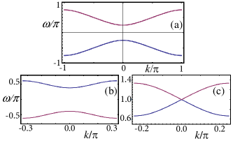
Figure 1: Dispersion relation (DR) of the 1D-QW for $\theta=\pi/4$ (a); effective DRs of the 1D-EQW for $\varphi=2\pi/p$ with $p=3$ (b) and $p=4$ (c).

When $\varphi/2\pi=q/p$ there must exist a stroboscopic QW within the EQW, which has been cleverly exploited by Cedzich et al. Cedzich13 in order to derive an effective dispersion relation for the EQW. Their result reads Cedzich13

$$\left.\cos\omega_{\pm}\left(k\right)\right|_{p}^{\left(odd\right)} = c_{\theta}^{p}\cos pk,$$ (6)

$$\left.\cos\omega_{\pm}\left(k\right)\right|_{p}^{\left(even\right)} = \left(1-c_{\theta}^{p}\right)\left(-1\right)^{1+\frac{p}{2}}-c_{\theta}^{p}\cos pk,$$ (7)

with $c_{\theta}\equiv\cos\theta$, see Fig. 1 (see Appendix A and the treatment below of the alternate walk for details). The effective group velocities are computed with $v_{g}\left(k\right)=p^{-1}\partial\omega\left(k\right)/\partial k$, and it is easy to show that the maximum velocities are given by $v_{g}^{\max}=\pm c_{\theta}^{p}$ for odd $p$ (ocurring at $k=\pi/2p$), and $v_{g}^{\max}=\mp\sqrt{c_{\theta}^{p}}$ for even $p$ (ocurring at $k=0$ for $p=4n$ and $k=\pi/p$ for $p=4n+2$ with $n$ an integer). Notice that now the pseudo-momentum $k$ runs from $-\pi/p$ to $+\pi/p$. It is clear that $v_{g}^{\max}$ rapidly decreases as $p$ increases, hence one expects to see a transient trapping of the probability distribution, the larger $p$ the longer its duration, the trapping being imperfect because the maximum group velocities, even if small, are not null. This is consistent with the view of Landau-Zener transitions becoming less important when the phase jumps are smaller Regensburger11 but notice that given the discrete nature of the walk, the (transient) localization can also occur for sizeable values of $\varphi$.

Consider now the irrational case. Any irrational number can be approximated, with arbitrary accuracy, by the rational number obtained after a suitable truncation of the irrational’s continued fraction expansion

$$\frac{\varphi}{2\pi}=\left\{a_{0},a_{1},a_{2}\ldots\right\}\equiv a_{0}+\frac{1}{a_{1}+\frac{1}{a_{2}+\ldots}}.$$ (8)

Hence the irrational is approximated to some rational when the expansion is finite, the closer is the approximation the more terms the expansion contains Cedzich13 . This means that we can infer the behaviour for the EQW in the irrational case by thinking about what occurs with its successively more precise rational approximations. However, one must keep in mind that in real situations (measurements, computations) rationals and irrationals cannot be distinguished, as the number of available digits is always finite.

Consider first the rational case $\varphi/2\pi=\left\{0,a_{1}\right\}=1/m_{1}$. From the arguments above, one expects the existence of some periodicity in the evolution of the probability distribution, and this is indeed the case: it oscillates with a period $m_{1}$ when $m_{1}$ is odd, and with a period $2m_{1}$ when $m_{1}$ is even (the difference between even and odd cases lies in that the walker needs two steps for repeating any position).

Consider now the rational $\left\{0,a_{1},a_{2}\right\}=n_{2}/m_{2}$ where $n_{2}=a_{2}$ and $m_{2}=1+a_{1}a_{2}$. Numerics reveal two periods in the evolution of the distribution width, one period $m_{2}$ and also a period $m_{1}$ reminiscent of the case $\left\{0,a_{1}\right\}$. For larger sequences $\left\{0,a_{1},a_{2},a_{3},\ldots\right\}$ the tendency is the same, with more periods that can be numerically observed and that correspond to the periods of the subsequent possible truncations of the sequence. Of course the weights of the different terms $a_{n}$ determine the details of the dynamics, as periods with very different orders of magnitude can be simultaneously involved and, depending on the particular case, the periods are or not easily seen.

As stated, the continued fraction expansion of an irrational number must contain an infinite number of terms. Hence, in very general terms, one would expect to see manifestations of all the periods (there are an infinite number of them) contained in the successive possible truncations of the irrational expansion, leading to a quite complicated dynamics in general that, in any case, manifests as a permanent trapping. The numerics confirm this and support the conclusion that the probability distribution is really trapped for irrational values of $\varphi/2\pi$. This is the fundamental difference between the rational and the irrational cases: for rationals trapping is transient and lasts more the larger $p$ is, while for irrationals the trapping is permanent. We direct the reader to the thorough study of Cedzich et al. for full details Cedzich13 .

III Electric QWs in 2D

Unlike the 1D case, completely characterized by only four parameters –of which only two $\left(\theta,\varphi\right)$ are dynamically relevant–, in the 2D case the number of possible independent parameters is actually too large to try any general treatment. Multidimensional QWs were first introduced by Mackay et al. Mackay02 who generalized the 1D definition by endorsing the walker with a $2N$-dimensional qudit, and different walks are defined depending on the $2N\times 2N$ coin operator. The most widely used and studied 2D-QW is the so-called Grover walk, whose electric version we will consider first.

In 2D-QWs the walker moves on a 2D lattice and is endorsed with a four-dimensional coin–qudit, the evolution being governed by $\left|\psi\left(t+1\right)\right\rangle=\hat{S}_{2}\hat{C}_{2}\left|\psi\left(t\right)\right\rangle$ with $\hat{S}_{2}$ the conditional 2D-shift and $\hat{C}_{2}$ a coin operator acting on the four–dimensional qudit. The state of the system at (discrete) time $t$ can be written as

$$\left|\psi\left(t\right)\right\rangle=\sum_{x,y}\sum_{s}a_{x,y,s}\left(t\right)\left|x,y;s\right\rangle.$$ (9)

Here $\left|x,y;s\right\rangle=\left|x,y\right\rangle\otimes\left|s\right\rangle$ with $\left|x,y\right\rangle$ the state of the walker on the 2D lattice and $\left|s\right\rangle$ the coin-qudit. We take the ordering $s=X_{+},Y_{-},Y_{+},X_{-}$ for $s=1$ to $4$, respectively. (We refer the reader to Appendix B for a brief comment about that.) The conditional displacement in 2D reads

$$\hat{S}_{2} = \sum_{x,y}\sum_{j=\pm 1}[\left|x+j,y;X_{j}\right\rangle\left\langle x,y;X_{j}\right|$$ (10)

$$+\left|x,y+j;Y_{i}\right\rangle\left\langle x,y;Y_{j}\right|],$$

and the coin operator can be any unitary on the 4D coin Hilbert space.

III.1 The Grover 2D-EQW

For the Grover walk the coin operator matrix elements are

$$\left\langle j\right|\hat{C}_{G}\left|k\right\rangle=\frac{1}{2}-\delta_{jk},$$ (11)

with $j,k=X_{\pm},Y_{\pm}$. Grover’s walk dispersion relations consist of four sheets, two of which are plane (i.e. have a null group velocity for all $k$-values within the BZ), while the other two, non–flat, curves cross at five conical intersections located at the center and corners of the first BZ (see below the comments to the 2D alternate walk). The Grover walk is well known and we refer the reader to Hinarejos13 and references therein for further details.

We straightforwardly add the electric field to the Grover walk by using the unitary

$$\hat{U}_{\varphi_{x},\varphi_{y}}=e^{i\varphi_{x}\hat{x}}e^{i\varphi_{y}\hat{y}}\hat{S}_{2}\hat{C}_{G}.$$ (12)

Note that $e^{i\varphi_{x}\hat{x}}$ and $e^{i\varphi_{y}\hat{y}}$ commute with both $\hat{S}_{2}$ and $\hat{C}_{G}$.

While we have not been able to derive analytical results for the electric Grover walk, we have arrived to a series of conclusions from an extensive numerical study. First we choose the symmetric initial condition for which the Grover and Alternate walks are equivalent DiFranco11 ; Hinarejos13 (see next subsection), i.e. our initial condition does not project onto the non-propagating sheets of the dispersion relation. This initial state is $\left|c_{0}\right\rangle=2^{-1}\left(1,-1,-1,1\right)$ and in Fig. 2(a) a snapshot of the probability distribution at $t=600$ is shown. (Later on we comment on the effect of changing the initial coin state.)

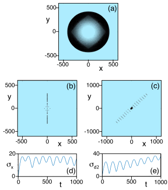
Figure 2: Grover-EQW. Top view of the probability distribution in the absence of electric field (a), and for electric fields $\varphi_{y}=0$ and $\varphi_{x}=2\pi/120$ (b) and $\varphi_{x}=\varphi_{y}=2\pi/120$ (c); where the probabitlity is higher in the darker regions. Figs. (d) and (e) show the evolution of the probability distribution standard deviation along the direction in which the trapping is larger for the cases (b) and (c), respectively. In all cases the initial coin state is $\left|c\right\rangle=\left(\left|X_{+}\right\rangle-\left|Y_{-}\right\rangle-\left|Y_{+}\right\rangle+\left|X_{-}\right\rangle\right)/2=1/2\left(1,-1,-1,1\right)$ and the walker is initially located at the origin. This initial state does not project onto the non-propagating branches of the dispersion relation, notice the absence of localization in (a), hence the localization effect is entirely due to the electric field. In (a) and (b) $t=600$ while in (c) $t=1000$.

From that learned in the 1D-EQW one could expect that for $\varphi_{x}=0$ and $\varphi_{y}\neq 0$ (an electric field along the $y$-axis) there could be a trapping effect, even if transient, along the $y$-axis, but not necessarily so along the $x$-axis. The same reasoning holds for the $\varphi_{y}=0$ case mutatis mutandi. This is so because the walker moves along the principal axes (the walker moves, after one step, from (0,0) to sites $(\pm 1,0)$ and $(0,\pm 1)$, this is not necessarily so for other walks), hence the directions of displacement of the walker coincide with those of the applied electric field and its orthogonal. This is indeed what the numerical solutions show, see Fig. 2(b), where a snapshot of the probability distribution is shown for $\varphi_{x}=2\pi/120$ (see caption for details), and Fig. 2(d) that shows the evolution of the distribution width (s.d.) along the $x$-axis, $\sigma_{x}$. The figure reveals a clear localization that can be intuitively understood as commented.

When the electric field is oriented along a line different from the principal axes things become different. For $\varphi_{x}=\varphi_{y}=\varphi$ (i.e., an electric field directed along the principal diagonal) one could expect two different scenarios: (i) a localization along the principal diagonal (the direction of the field) and a spreading of the distribution along the anti-diagonal (similarly to the axial field case discussed above); but one could also expect (ii) a localization effect along both the $x$ and $y$ axes (hence an effective 2D localization) if one thinks that the projection of the field along $x$ ($y$) will provoke a localization along $x$ ($y$). However, the fact that the walker moves, after each step, along the principal axes excludes the first possibility because the field direction does not coincide with the natural directions of displacement of the walker, hence the second option should be closer to what actually occurs.

Even if this is not entirely the case, it is quite close to it as can be seen in Figs. 2(c) and 2(e) where we show the probability distribution and its width for $\varphi_{x}=\varphi_{y}=2\pi/120$. It can be appreciated how most of the probability distribution remains localized, but for some bursts that, so to say, periodically escape from the trapping region, the bursts being apparent in Fig. 2(c). The origin of these imperfections in the 2D-localization can be traced back to the existence of critical points in the Grover walk, as around these points interband transitions cannot be avoided. We delay the discussion about that to our study of the alternate walk below.

For other inclinations of the field we have observed complicated dynamics, with the probability distribution usually alligning with some non-trivial direction with respect to the electric field. See an example below, Fig. 5, when we consider the electric alternate walk.

We must mention that for initial states other from the one we have chosen (the one that makes the Grover walk equivalent to the alternate walk in 2D DiFranco11 ), the behaviour is qualitatively the same, and the main difference is the existence of a more or less large amount of trapping originated not by the electric field, but by the projections of the initial condition onto the non-propagating branches of the dispersion relation. Notice that these branches are not affected by the electric field, so that the population that is trapped in those branches would remain trapped.

As for the influence of the value of $\varphi$, we have observed that the smaller it is the longer time the localization remains, as in the 1D case, but we have not seen any clear difference between rationals and “irrationals”. This could have also been expected, however, because in a 2D walk the trajectories that the walker can follow are not forced to run parallel to the direction of the electric field, as is obviously the case in the 1D walk, hence the dependence on the size of the phase cannot be that critical as in the 1D case.

Before moving to other 2D walks, let us recall here that the Grover walk can also be understood as the 1D walk of two independent and non-interacting bosons. In this case, the localization along an axis of the walk when the field is applied along that axis would mean that the electric field acts directly only on one particle, with the result that this particle remains at rest (during the transient localization, of course) while the other particle on which no electric field acts, follows a quantum walk. On the other hand, when the field acts equally on the two particles (case $\varphi_{x}=\varphi_{y}$) we see a (transient) co-walking of the particles as if they formed a molecule Albrecht12 .

III.2 Electric Alternate QWs in 2D

The Alternate Quantum Walk (AQW) was introduced as a simpler way to build a QW on a 2D lattice using lower dimensional qudit resources than those needed in the standard 2D walk DiFranco11 ; DiFranco11b ; Roldan13 .

Consider a quantum walker on a 2D–lattice with a 1D internal qubit, the basis states being $\left|x,y;s\right\rangle$ with $s=\pm 1$. In the electric alternate QW in 2D (EAQW) the state evolves as $\left|\psi\left(t+1\right)\right\rangle=\hat{U}_{\varphi_{1},\varphi_{2}}\left|\psi\left(t\right)\right\rangle$ where

$$\hat{U}_{\varphi_{1},\varphi_{2}}\equiv e^{i\left(\varphi_{x}\hat{x}+\varphi_{y}\hat{y}\right)}\hat{U}_{0,0}=e^{i\left(\varphi_{x}\hat{x}+\varphi_{y}\hat{y}\right)}\hat{S}_{y}\hat{C}_{y}\hat{S}_{x}\hat{C}_{x}.$$ (13)

being $\hat{S}_{j}$ the conditional displacement along axis $j=x,y$, and $\hat{C}_{j}$ given by (3) with $\alpha=\beta$, and with, in general, different angles $\theta_{x}$ and $\theta_{y}$. As in the electric Grover walk, we can set the two phases $\varphi_{x}$ and $\varphi_{y}$ together at the end of the operator because of compatibility.

For $\varphi_{x}=\varphi_{y}=0$, the usual alternate QW DiFranco11 ; DiFranco11b is recovered, whose dispersion relations Roldan13 are

$$\cos\omega_{\pm} = \cos\left(k_{x}+k_{y}\right)\cos\theta_{x}\cos\theta_{y}$$ (14)

$$-\cos\left(k_{x}-k_{y}\right)\sin\theta_{x}\sin\theta_{y}.$$

In the usual case $\hat{C}_{x}=\hat{C}_{y}=\hat{H}$ (i.e., when the two coins are Hadamard transformations) the dispersion relations show a gap-less band structure with conical intersections (diabolical points), Fig. 3(a). (The implications in the evolution of the system of these conical intersections has been analyzed in detail in Roldan13 ; Hinarejos13 .) These dispersion relations, if rotated by $\pi/4$, are the same as the two non–plane sheets of the Grover’s 2D walk dispersion relations; hence, if an initial condition is chosen (in the Grover’s walk) such that it does not project on the plane sheets, the Grover walk and the alternate walks become equivalent in 2D except for the $\pi/4$ rotation of the walk axes Roldan13 . This is what we did in the previous section.

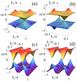
Figure 3: Dispersion relations of the AQW in 2D (a), and effective dispersion relations of the AEQW with $\varphi_{x}=2\pi/p$ and $\varphi_{y}=0$ for $p=9$ (b) and $p=8$ (c) and (d). In (b) and (c) we have taken $\theta_{1,2}=\pi/4\pm\delta\theta$ with $\delta\theta=0$, while in (d) $\delta\theta=0.05$.

Consider now the simplest case of an electric field directed along one of the principal axes, say $\varphi_{y}=0$. We reason along the same lines as in the 1D case Cedzich13 and first show that $\hat{U}_{\varphi_{x},0}^{p}$ is translational invariant when $\varphi_{x}=2\pi q/p$: It is easy to see that

$$\hat{U}_{\varphi_{x},0}\left(k_{x},k_{y}\right)\left|\psi\left(k_{x},k_{y}\right)\right\rangle=$$

$$\hat{U}_{0,0}\left(k_{x}+\varphi_{x},k_{y}\right)\left|\psi\left(k_{x}+\varphi_{x},k_{y}\right)\right\rangle,$$ (15)

from which a similar reasoning to that in the 1D case Cedzich13 leads to

$$\hat{U}_{\varphi_{x},0}^{p}\left(k_{x},k_{x}\right) = \hat{U}_{0,0}\left(k_{x}+\varphi_{x},k_{y}\right)$$ (16)

$$\hat{U}_{0,0}\left(k_{x}+2\varphi_{x},k_{y}\right)\ldots U_{0,0}\left(k_{x}+p\varphi_{x},k_{y}\right)$$

$$= \hat{S}_{x}\hat{U}_{0,0}\left(k_{x},k_{y}\right)\hat{S}_{x}^{2}\hat{U}_{0,0}\left(k_{x},k_{y}\right)$$

$$\ldots\hat{S}_{x}^{p}\hat{U}_{0,0}\left(k_{x},k_{y}\right),$$

which has been written in a form suitable to apply the Lemma used by Cedzich et al. Cedzich13 (see Appendix A for details). Finally one gets the stroboscopic dispersion relations

$$\left.\cos\omega_{\pm}\left(k\right)\right|_{p}^{\left(odd\right)} = \left|r\right|^{p}\cos\left[p\arccos\left(\frac{\mathrm{Re}\left(r\right)}{\left|r\right|}\right)\right],$$ (17)

$$\left.\cos\omega_{\pm}\left(k\right)\right|_{p}^{\left(even\right)} = -\left|r\right|^{p}\cos\left[p\arccos\left(\frac{\mathrm{Re}\left(r\right)}{\left|r\right|}\right)\right]+$$ (18)

$$\left(-1\right)^{\frac{p}{2}+1}\left(1-\left|r\right|^{p}\right),$$

with

$$r=e^{ik_{x}}\left(c_{\theta_{x}}c_{\theta_{y}}e^{ik_{y}}-s_{\theta_{x}}s_{\theta_{y}}e^{-ik_{y}}\right),$$ (19)

and $s_{\theta_{x}}=\sin\theta_{x}$, etc. From $\omega_{\pm}\left(k\right)$ the group velocities are easily obtained as $v_{g}=(1/p)\partial\omega/\partial k$, we do not give them because of their length.

In Figs. 3 we represent these effective dispersion relations for $p=9$, Fig. 3(b), and $p=8$, Figs. 3(c) and (d); where we took $\theta_{x,y}=\pi/4\pm\delta\theta$ with $\delta\theta=0$ in (b) and (c), and $\delta\theta=0.05$ in (d). We have chosen small values for $p$ in order to easily visualize the curves, as the slopes quickly increase as $p$ does, and for larger $p$ it is difficult to see the details. We see that the conical intersections of the original dispersion relation survive with the electric field, and we see that a non–null $\delta\theta$ breaks these degeneracies Roldan13 . Hence one must expect large changes in the dynamics depending on whether $\delta\theta=(\theta_{x}-\theta_{y})/2$ is null or not. In any case, notice that for most $k$ values there are wide plateaus in the effective dispersion relations in which the group velocities are relatively very small. Moreover, the plateaus become wider as $p$ is increased, so that the smallness of the group velocity across most of the $k$-space is a most remarkable feature. Notice finally that $k_{y}$ now runs from $-\pi/2p$ to $\pi/2p$. Apart from these very general considerations, not much information can be extracted from the dispersion relations when the initial state is localized in space, as it is our present case, as the effect of interferences on the propagation of each frequency component cannot be easily devised.

In order to study numerically the behaviour of the EAQW it is convenient to make use of the partial equivalence with the Grover walk, keeping in mind the $\pi/4$ rotation between the two walks. This rotation reflects the fact that the directions of displacement of the walker do not coincide with the principal axes, but with the diagonals, as at each step the walker is displaced along both $x$ and $y$. This implies that when a field is added along, say, $y$, this actually means that the walker acquires a phase $\varphi$ at both $x$ and $y$ displacements, which is equivalent to the action of a field of amplitude $2\varphi$ directed along the main diagonal in the electric Grover walk.

The $\pi/4$ rotation manifests in the numerical results: The plots shown in Fig. 2 above for the Grover walk with fields of amplitude $\varphi$ along $x$, in Fig. 2(b), and along the main diagonal, in Fig. 2(c), apply to the EAQW with $2\varphi$ fields along the diagonal and along the $x$-axis, respectively, if rotated 45 degrees.

However the alternate walk allows one extra degree of freedom, because when $\theta_{x}$ is taken different from $\theta_{y}$, the conical degeneracies are removed, which allows to see their influence

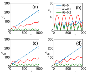
Figure 4: AEQW. Evolution of the probability distribution width along the principal axes, (a) and (b), and the diagonals, (c) and (d), for $\varphi_{x}=2\pi/120$ and $\varphi_{y}=0$. In all cases three different values of $\delta\theta$ ($=0$, $0.1$, and $0.2$; curves with higher to lower values at $t=1000$) have been considered, where $\theta_{x,y}=\pi/4\pm\delta\theta$.

In Figs. 4 we represent the evolution of the distribution width, along both the principal axes and the diagonals, for three values of $\delta\theta$ and for a field $\varphi_{x}=2\pi/120$ and $\varphi_{y}=0$. The case $\delta\theta=0$ reveals that there is a transient trapping along the $y$-axis. When the conical intersections are lifted for $\delta\theta\neq 0$ the progressive appearance of a perfect trapping along all four axes is clear. Again, this is consistent with the view that Landau-Zener transitions become less likely the larger is the energy gap.

We have also investigated the effect of tilted fields, and in Fig. 5 we show results for the case $\varphi_{x}=2\varphi_{y}=2\pi/120$. The figure reveals that also in this case there occurs a perfect trapping when $\delta\theta$ is large enough, which emphasizes the role played by the conical intersections.

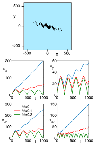
Figure 5: AEQW. Top figure is a snapshot of the probability distribution for $\varphi_{x}=2\varphi_{y}=2\pi/120$ at $t=600$. The rest of the figures show, as in Fig. 4, the evolution of the probability distribution width.

III.3 Other EQWs in 2D: DFT and Hadamard coins

As deriving general analytical results with electric fields is beyond reach in this case, looking at the walk dispersion relation seems the obvious simple choice, as if they contain diabolical points one can expect a behaviour similar to that of the Grover walk, while a perfect 2D trapping for some appropriate field direction could be expected when there are no conical intersections.

Let us consider first the 2D-DFT walk, whose coin reads

$$\hat{C}_{DFT}=\frac{1}{2}\left(\begin{array}[]{cccc}1&1&1&1\\ 1&i&-1&-i\\ 1&-1&1&-1\\ 1&-i&-1&i\end{array}\right).$$ (20)

The dispersion relations are not explicit and are obtained by numercically solving

$$\cos 2\omega+2\sin 2\omega=\cos\left(k_{x}-k_{y}\right)+$$

$$2\left(\sin\omega+\sin k_{x}+\sin k_{y}+\cos k_{x}+\cos k_{y}\right)\sin\omega$$ (21)

see Fig. 6. It consists of four sheets with several conical intersections and a lesser degree of symmetry than the Grover walk. In Fig. 6(b) we have represented the probability distribution at $t=600$, see caption.

The effect of the electric field on the DFT-walk is similar to that in the Grover walk, at least qualitatively, as it can be seen by comparing Figs. 7 and 2. Clearly the trapping capacity when the field is along the diagonal is much smaller in the DFT coin. Hence, we conclude that the electric-DFT walk is very similar to the electric Grover-walk, the differences beeing more quantitative than qualitative.

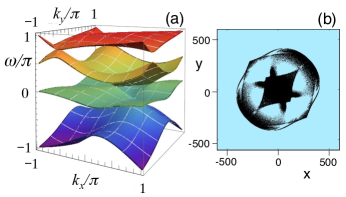
Figure 6: Dispersion relation of the DFT-QW in 2D (a), and a snapshot of the probability distribution at $t=600$ (b). The initial coin state is $\left|c\right\rangle=1/2\left(1,i,i,-1\right)$.

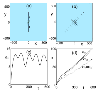
Figure 7: Electric DFT walk in 2D. In Figs. (a) and (c) the electric field is $\varphi_{x}=2\pi/120$ and $\varphi_{y}=0$, whilst in Figs. (b) and (d) the electric field is $\varphi_{x}=\varphi_{y}=2\pi/120$. The initial state is as in Fig. 6 and $t=600$.

Let us finally consider the Hadamard walk, whose coin is defined as $\hat{C}_{H_{2}}=\hat{H}\otimes\hat{H}$, i.e.

$$\hat{C}_{H_{2}}=\frac{1}{2}\left(\begin{array}[]{cccc}1&1&1&1\\ 1&-1&1&-1\\ 1&1&-1&-1\\ 1&-1&-1&1\end{array}\right),$$ (22)

which is a separable coin when acting on vector $\left|s\right\rangle=\mathrm{col}(X_{+},Y_{-},Y_{+},X_{-})$ Mackay02 (see Appendix B). Its dispersion relation reads Annabestani10

$$\cos\omega_{1,2} = \frac{1}{4}\left[\cos k_{x}-\cos k_{y}\mp\sqrt{\mathcal{S}+8}\right],$$ (23)

$$\mathcal{S} = \cos^{2}k_{x}+\cos^{2}k_{y}+6\cos k_{x}\cos k_{y},$$ (24)

and its four sheets can be seen in Fig. 8, that appear distributed by pairs that intersect along a line within each pair, but the two pairs are well separated by a clear gap.

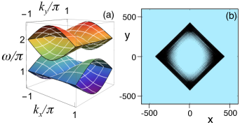
Figure 8: Dispersion relation of the Hadamard-QW in 2D (a), and snapshot of the probability distribution at $t=600$ (b). The initial coin state is $\left|c\right\rangle=1/2\left(1,i,i,-1\right)$.

The effect of the electric field on this walk is sharper than in any of the previous ones but the alternate walk with different angles in the two coin operations. Now we see clear 1D or 2D trapping depending on the direction of the field as Figs. 9 and 10 illustrate. Figs. 9 show the behaviour for a field directed along the main diagonal, which produces a sharp diagonal trapping, while in Fig. 10 it is shown how a field directed along the $x$-axis produces a sharp 2D trapping. The behaviour reveals that in this Hadamard walk the main directions of propagation do not coincide with those of the main axes. The 2D-Hadamard electric walk confirms the role played by conical intersections in the dispersion relations leading to the conclussion that perfect 2D trapping can occur if such diabolical points are removed.

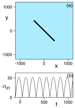
Figure 9: Electric Hadamard-QW in 2D when the electric field is $\varphi_{x}=2\pi/120$ and $\varphi_{y}=0$. (a) shows a snapshot of the probability distribution at $t=1000$, and (b) the evolution of its width. The initial coin state is $\left|c\right\rangle=1/2(1,i,i,-1)$.

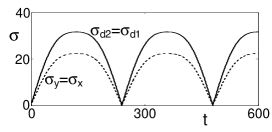
Figure 10: Evolution of the probability distribution width for the electric Hadamard-QW in 2D when the electric field is $\varphi_{x}=\varphi_{y}=2\pi/120$. A perfect 2D trapping is apparent.

IV Conclusions

After a suitable review of the one dimensional case, we have addressed the study of electric quantum walks in two dimensions. The easiest one to understand in intuitive terms is the Grover walk: a field along the principal axes produces trapping along the field axis, and when the field acts along the diagonals, a frustrated 2D trapping occurs. The reason for the frustration lies in the existence of conical intersections in the Grover walk dispersion relations, which we have confirmed through the analysis of the alternate electric QW. As the two walks are equivalent after a $\pi/4$ rotation of the principal axes, the behaviour of the alternate electric walk is somewhat counter-intuitive at first sight as the field seems to be rotated by $\pi/4$. We have also addressed the two other popular 2D walks, namely the Hadamard and DFT walks.

In our analysis of the alternate walk we have shown that when the two coin operations within each step are not identical, which removes conical intersections, the effect of the electric field can lead to a perfect 2D localization, a result confirmed by the behaviour of the Hadamard walk that exhibits perfect 2D trapping for appropriate field direction.

Acknowledgements

We gratefully acknowledge continued financial support from Spanish Government (Ministerio de Educación e Innovación) through projects FIS2011-26960, FIS2014-60715-P, FPA2011-23897, FPA2014-54459-P, and SEV-2014-0398, and support from the Generalitat Valenciana (Valencian Goverment) through grant GV-PROMETEO-II-2014-087. MH acknowledges financial support from ANII (Uruguay) grant PD_NAC_2014_1_102359.

V Appendix A

Cedzich et al. Cedzich13 introduce the following Lemma. Let $m\in\mathbb{N}$ and let $\eta$ be a primitive $m$-th root of unity. Now consider the matrices

$$\hat{A}=\left(\begin{array}[]{cc}a&b\\ c&d\end{array}\right),\ \ \hat{R}=\left(\begin{array}[]{cc}\eta&0\\ 0&\eta^{-1}\end{array}\right),$$ (25)

and set

$$\tau_{m}=Tr\left[\hat{A}\hat{R}^{0}\hat{A}\hat{R}^{1}\ldots\hat{A}\hat{R}^{m-1}\right],$$ (26)

then it can be demonstrated that

$$\tau_{m}^{\left(odd\right)} = a^{m}+d^{m},$$ (27)

$$\tau_{m}^{\left(even\right)} = -\left(a^{m}+d^{m}\right)+2\left(-1\right)^{m/2}$$ (28)

$$\times\left[\left(ad\right)^{m/2}-\left(\det A\right)^{m/2}\right].$$

In order to apply the Lemma we need the matrix elements of $\hat{U}_{0,0}\left(k_{x},k_{y}\right)$, wich can be written as

$$\hat{U}_{0,0}\left(k_{x},k_{y}\right)=\left(\begin{array}[]{cc}a&b\\ -b^{\ast}&a^{\ast}\end{array}\right),$$ (31)

$$a=e^{i\left(k_{x}+k_{y}\right)}\cos\theta_{x}\cos\theta_{y}-e^{i\left(k_{x}-k_{y}\right)}\sin\theta_{x}\sin\theta_{y},$$ (32)

$$b=e^{i\left(k_{x}+k_{y}\right)}\sin\theta_{x}\cos\theta_{y}+e^{i\left(k_{x}-k_{y}\right)}\cos\theta_{x}\sin\theta_{y},$$ (33)

and then from the trace $\tau_{p}=a^{p}+\left(a^{\ast}\right)^{p}$ one gets the dispersion relations

$$\left.\cos\left[\omega_{\pm}\left(k\right)\right]\right|_{p}^{\left(odd\right)} = \left|a\right|^{p}\cos\beta,$$ (34)

$$\left.\cos\left[\omega_{\pm}\left(k\right)\right]\right|_{p}^{\left(even\right)} = \left(-1\right)^{\frac{p}{2}+1}\left(1-\left|a\right|^{p}\right)-\left|a\right|^{p}\cos\beta,\qquad$$ (35)

$$\beta \equiv p\arccos\left(\frac{\mathrm{Re}\left(a\right)}{\left|a\right|}\right).$$ (36)

VI Appendix B

Multidimensional QWs can be defined in different ways. In the original definition Mackay02 the ordering of the coin elements is taken from the tensor product of two qubits: if $\mathrm{col}\left(x_{+},x_{-}\right)$ and $\mathrm{col}\left(y_{+},y_{-}\right)$ are these qubits, then the tensor product qudit has elements $\mathrm{col}\left(x_{+}y_{+},x_{+}y_{-},x_{-}y_{+},x_{-}y_{-}\right)$.

It is natural to interpret $x_{+}y_{+}$ ($x_{-}y_{-}$) as the positive (negative) direction of the main diagonal and $x_{+}y_{-}$ ($x_{-}y_{+}$) as the negative (positive) direction of the antidiagonal, so that one can write the coin vector components as $\mathrm{col}\left(d_{+},a_{-},a_{+},d_{-}\right)$ with $d$ ($a$) standing for diagonal (antidiagonal). This is the ordering chosen by, e.g., Mackay02 . However the above choice seems to leave unoccupied positions on the plane, and it is also natural to avoid this by rotating clockwise the displacement directions by 45º, so that the coin vector is written as $\mathrm{col}\left(x_{+},y_{-},y_{+},x_{-}\right)$, which is the choice made, e.g., by Annabestani10 and that we have also followed. Of course the two choices are equivalent, but for a 45º rotation.

But the above orderings are not mandatory and one can order the coin components at will. For example, in Hinarejos13 we chose the ordering $\mathrm{col}\left(x_{+},x_{-},y_{+},y_{-}\right)$, mainly because it admits a straightforward notation in the generalization to higher dimensional QWs.

This can be confusing, of course, as authors do not use to specify which ordering have they chosen, which makes sometimes difficult to translate the results of different articles. For example, if one uses the definitions of Mackay02 ; Annabestani10 , the Hadamard coin expression is that given in the main text, Eq. (22), that is designed to be a separable matrix, but if the same matrix is applied to other ordering, e.g. ours in Hinarejos13 , then one is not implementing a separable operator, and one is indeed making a different QW. In fact, if one is willing to implement the Hadamard walk with the ordering of the coin elements in Hinarejos13 , the correct matrix must be written as

$$\hat{C}_{H^{\prime}}=\frac{1}{2}\left(\begin{array}[]{cccc}1&1&1&1\\ 1&1&-1&-1\\ 1&-1&-1&1\\ 1&-1&1&-1\end{array}\right),$$ (37)

which is obtained by permuting the second and fourth indexes of matrix (22), as this is the difference between the two orderings we have discussed. It is fortunate the fact that the Grover coin has the same expression irrespectively of the ordering chosen for the coin vector elements.

References

- (1) J. Kempe, Contemp. Phys. 44, 307 (2003).
- (2) V. Kendon, Math. Struct. Comput. Sci. 17, 1169 (2006); Phil. Trans. R. Soc. A 364, 3407 (2006).
- (3) N. Konno, Quantum Walks in Quantum Potential Theory (Lecture Notes in Mathematics vol 1954) ed U Franz and M Schürmann (Berlin: Springer, 2008) pp 309–452.
- (4) S.E. Venegas-Andraca, Quant. Inf. Proc. 11, 1015 (2012).
- (5) F. W. Strauch, Phys. Rev. A 73, 054302 (2006).
- (6) G.J. de Valcárcel, E. Roldán, and A. Romanelli, New J. Phys 12, 123022 (2010).
- (7) M. Hinarejos, A. Pérez. E. Roldán, A. Romanelli, and G.J. de Valcárcel, New J. Phys. 15, 073041 (2013).
- (8) F. W. Strauch, J. Math. Phys. 48, 082102 (2007).
- (9) C.M. Chandrasekar, Sci. Reports Sci. Rep. 3, 2829 (2013).
- (10) G. Di Molfetta, M. Brachet, and F. Debbasch, Physica A 397, 157 (2014).
- (11) Y. Aharonov, L. Davidovich, and N. Zagury, Phys. Rev. A 48, 1687 (1993).
- (12) D. Meyer, J. Stat. Phys. 85, 551 (1996).
- (13) E. Farhi and S. Gutmann, Phys. Rev. A 58, 915 (1998).
- (14) A.M. Childs and J. Goldstone, Phys. Rev. A 70, 042312 (2004).
- (15) Richard P. Feynman and A.R. Hibbs, Quantum Mechanics and Path Integrals, International Series in Pure and Applied Physics (McGraw-Hill, 1965).
- (16) J. Watrous, Proceedings of the 33rd Annual ACM Symposium on the Theory of Computing, Heraklion, Crete, Greece, July 06–08, 2001 (ACM Press, New York, 2001), p.60.
- (17) A.M. Childs, Phys. Rev. Lett. 102, 18050 (2009).
- (18) N.B. Lovett, S. Cooper, M. Everitt, M. Trevers, and V. Kendon, Phys. Rev. A 81, 042330 (2010).
- (19) K. Manouchehri and J. Wang, Physical Implementation of Quantum Walks (Springer, 2014).
- (20) D. Bouwmeester, I. Marzoli, G. P. Karman, W. Schleich, and J. P. Woerdman, Phys. Rev. A 61, 013410 (1999).
- (21) P. L. Knight, E. Roldán, and J. E. Sipe, Phys. Rev. A 68, 020301 (2003); Opt. Commun. 227, 147 (2003).
- (22) E. Roldán and J. C. Soriano, J. Mod. Opt. 52, 2649 (2005).
- (23) P. Arnault and F. Debbasch, Physica A 443, 179 (2016).
- (24) I. Yalçınkaya and Z. Gedik, Phys. Rev. A 92, 042324 (2015).
- (25) A. Wojcik, T. Lukzak, P. Kurzynski, A. Grudka, and M. Bednarska, Phys. Rev. Lett. 93, 180601 (2004).
- (26) D. A. Meyer, Phys. Rev. E 55, 5261 (1997).
- (27) D. A. Meyer, J. Phys. A: Math. Gen. 31, 2321 (1998).
- (28) M.C. Bañuls, C. Navarete, A. Pérez, E. Roldán, and J.C. Soriano, Phys. Rev. A 73, 062304 (2006).
- (29) A. Regensburger, Ch. Bersch, B. Hinrichs, G. Onishchukov, A. Schreiber, Ch. Silberhorn, and U. Peschel, Phys. Rev. Lett. 107, 233902 (2011).
- (30) C. Cedzich, T. Rybár, A. H. Werner, A. Alberti, M. Genske, and R. F. Werner, Phys. Rev. Lett. 111, 160601 (2013).
- (31) M. Genske, W. Alt, A. Steffen, A. H. Werner, R. F. Werner, D. Meschede, and A. Alberti, Phys. Rev. Lett. 110, 190601 (2013).
- (32) P. Xue, R. Zhang, H. Qin, X. Zhan, Z.H. Bian, J. Li, and B.C. Sanders, Phys. Rev. Lett. 114, 140502 (2015).
- (33) N. Linden and J. Sharam, Phys. Rev. A 80, 052327 (2009).
- (34) Y. Shikano and H. Katsura, Phys. Rev. E 82, 031122 (2010).
- (35) D. R. Hofstadter, Phys. Rev. B 14, 2239 (1976).
- (36) C. Di Franco and M. Paternostro, Phys. Rev. A 91, 012328 (2015).
- (37) S. John , Phys. Rev. Lett. 58, 2486 (1987); E. Yablonovitch, Phys. Rev. Lett. 58, 2059 (1987).
- (38) T.D.Mackay, S.D. Bartlett,L.T.Stephenson, and B. C. Sanders, J. Phys. A: Math. Gen. 35, 2745 (2002).
- (39) A. Ahlbrecht, A. Alberti, D. Meschede, V.B. Scholz, A.H. Werner, and R.F. Werner, New J. Phys. 14, 073050 (2012).
- (40) C. Di Franco, M. Mc Gettrick, and Th. Busch, Phys. Rev. Lett. 106, 080502 (2011).
- (41) C. Di Franco,M.Mc Gettrick, T. Machida, and Th. Busch, Phys. Rev. A 84, 042337 (2011).
- (42) E. Roldán, C. Di Franco, F. Silva, and G.J. de Valcárcel, Phys. Rev. A 87, 022336 (2013).
- (43) B. Kollár, J. Novotný, T. Kiss, and I. Jex, New J. Phys. 16, 023002 (2014).
- (44) M. Annabestani, M. R. Abolhasani, and G. Abal, J. Phys. A: Math. Theor. 43, 075301 (2010).