Energy Bounds for a Compressed Elastic Film on a Substrate

Abstract

We study pattern formation in a compressed elastic film which delaminates from a substrate. Our key tool is the determination of rigorous upper and lower bounds on the minimum value of a suitable energy functional. The energy consists of two parts, describing the two main physical effects. The first part represents the elastic energy of the film, which is approximated using the von Kármán plate theory. The second part represents the fracture or delamination energy, which is approximated using the Griffith model of fracture. A simpler model containing the first term alone was previously studied with similar methods by several authors, assuming that the delaminated region is fixed. We include the fracture term, transforming the elastic minimization into a free-boundary problem, and opening the way for patterns which result from the interplay of elasticity and delamination.

After rescaling, the energy depends on only two parameters: the rescaled film thickness, $\sigma$, and a measure of the bonding strength between the film and substrate, $\gamma$. We prove upper bounds on the minimum energy of the form $\sigma^{a}\gamma^{b}$ and find that there are four different parameter regimes corresponding to different values of $a$ and $b$ and to different folding patterns of the film. In some cases the upper bounds are attained by self-similar folding patterns as observed in experiments. Moreover, for two of the four parameter regimes we prove matching, optimal lower bounds.

1 Introduction

Compressed elastic sheets such as plastic films and fabric often exhibit self-similar folding patterns. A typical example are folds in curtains, which decrease in number and increase in size from top to bottom as the folds merge. This coarsening phenomenon is also observed at the microscale in graphene and semiconductor films. The spontaneous delamination of prestrained semiconductor films from their substrates produces blisters with rich, self-similar folding patterns [19]. This also represents a challenge to manufacturers. Recently experimentalists have discovered how this, originally unwanted phenomenon, can be harnessed for thin film patterning and nanofabrication [21], for example to create nanotubes and nanochannels from prestrained semiconductor films [11], [27].

In the mathematical community there is an ongoing programme to understand why these patterns occur. The calculus of variations has proved to be a useful tool, where the patterns are viewed as minimisers of an elastic potential energy. This is the approach we take in this paper.

Motivated by the experiments of [27], we study a variational model of a two-layer material consisting of a rectangular elastic film on a substrate. The film is clamped along one edge to the substrate and is free on the other three sides. Due to a lattice mismatch between the film and the substrate, the film suffers isotropic in-plane compression. It can relax this compression by delaminating from the substrate and buckling, but a short-range attractive force between the film and the substrate opposes this. We assign to the material the following energy:

(1.1) $$I^{(\sigma,{\gamma})}:=I_{\textrm{vK}}+I_{\textrm{Bo}},$$

where $I_{\textrm{vK}}$ is the von Kármán energy of isotropically compressed plates:

(1.2) $$I_{\textrm{vK}}[\mathboit u,w,l_{1},l_{2}]:=\int_{0}^{l_{1}}\!\int_{0}^{l_{2}}|D\mathboit u+(D\mathboit u)^{\mathrm{T}}+Dw\otimes Dw-\mathrm{Id}|^{2}\,dx\,dy+(\sigma l_{1})^{2}\int_{0}^{l_{1}}\!\int_{0}^{l_{2}}|D^{2}w|^{2}\,dx\,dy$$

and $I_{\textrm{Bo}}$ is a bonding energy that penalises delamination of the film from the substrate:

(1.3) $$I_{\textrm{Bo}}[\mathboit u,w,l_{1},l_{2}]:={\gamma}\,|\{(x,y)\in(0,l_{1})\times(0,l_{2})\,:\,w(x,y)>0\}|.$$

Here $(0,l_{1})\times(0,l_{2})$ is the set of material points of the film, $l_{1}\leq l_{2}$, and $\mathboit u(x,y)=(u(x,y),v(x,y))$ and $w(x,y)$ are the in-plane and vertical displacements of the film from an isotropically compressed state. The substrate is taken to be at height $z=0$ so that film is bonded to the substrate at points where $w=0$. The energy is rescaled so that $(u,v,w)=(x/2,y/2,0)$ corresponds to the stress-free, minimum energy state of the film, and $(u,v,w)=(0,0,0)$ has positive energy and corresponds to the isotropically compressed state. The energy has two parameters: $0<\sigma<1$ is the rescaled thickness of the film and ${\gamma}\geq 0$ is a measure of attractive force between the film and the substrate. We show how these are related to physical parameters such as the film thickness and Young’s modulus in Appendix A, where the energy (1.1) is derived. The experimental setup is shown in Figure 1 and discussed below.

Figure 1: Geometry of the partially delaminated film. The bottom layer is the substrate, the middle layer is the sacrificial buffer layer, which is removed by chemical etching in the region $x_{1}>0$, and the top layer is the thin elastic film. The film is subject to compression at the boundary $x_{1}=0$, where it is still attached to the buffer layer. It may rebond to the substrate in the region $x_{1}>0$. For simplicity, in our model we take the buffer layer to have zero thickness. Consequently we refer to the material as a two-layer material rather than a three-layer material. The general case is discussed briefly in Appendix B.

We assume that the film is clamped to the substrate along the edge $\{0\}\times(0,l_{2})$:

(1.4) $$u(0,y)=0,\quad v(0,y)=0,\quad w(0,y)=0,\quad Dw(0,y)=\mathbf{0}$$

and is free on the other three sides of the rectangle $(0,l_{1})\times(0,l_{2})$. Since the film cannot go below the substrate we also have the positivity constraint

(1.5) $$w\geq 0.$$

The von Kármán energy (1.2) is the sum of a stretching energy $I_{\textrm{S}}$, which penalises compression and extension, and a bending energy $I_{\textrm{Be}}$:

(1.6) $$I_{\textrm{S}} :=\int_{0}^{l_{1}}\!\int_{0}^{l_{2}}|D\mathboit u+(D\mathboit u)^{\mathrm{T}}+Dw\otimes Dw-\mathrm{Id}|^{2}\,dx\,dy,$$

$$I_{\textrm{Be}} :=(\sigma l_{1})^{2}\int_{0}^{l_{1}}\!\int_{0}^{l_{2}}|D^{2}w|^{2}\,dx\,dy.$$

The folding patterns in the experiments of [27], and in compressed thin films in general, can be explained as the competition between the stretching and bending energies. The stretching energy has no minimum over the set of displacements satisfying the clamped boundary condition. Its infimum is zero, and an infimising sequence can be constructed by taking a periodic folding pattern, with folds perpendicular to the clamped boundary, and by sending the wavelength of the folds to zero. This relaxes the compression in the film but sends the bending energy to infinity. The competition between the stretching and bending energies determines the scale of the pattern.

We shall see that for some range of the parameters $(\sigma,{\gamma})$ it is energetically favourable for the film to form a self-similar folding pattern with the wavelength of the folds increasing away from the clamped boundary. Close to the boundary a fine folding pattern is needed in order to interpolate the folds to the clamped boundary condition without paying too much stretching energy. It would cost too much bending energy, however, to use such small folds in the whole domain and so branching occurs to obtain larger folds in the bulk of the domain. The addition of the bonding energy, which is the novelty of this paper, complicates the situation further and gives a richer family of folding patterns.

Experimental Motivation.

In the experiments of [27] they use a three-layer material, where the bottom layer is a substrate (e.g., Si), the middle layer is a buffer layer (e.g., SiO₂), and the top layer is a thin semiconductor film (e.g., Si_xGe_1-x). Due to a lattice mismatch between the film and the buffer layer, the thin film suffers isotropic, in-plane compression. See Figure 1.

In the experiments, a slab of the buffer layer is removed by chemical etching. (An acid is used to eat away the buffer layer from the side, without damaging the film or substrate. Once the desired portion of the buffer layer has been removed the acid is washed out and the sample is dried.) This allows the thin film to partially relax the in-plane compression by folding. Since the buffer layer is thin, it is observed that the folds of the film come into contact with the substrate and bond to it via attractive interfacial forces. In this way submicro and nano scale channels are fabricated, which can be used, e.g., in nanofluidic devices. The patterns formed by the channels are self-similar, consisting of regions where the film is bonded to the substrate between folds that branch as they approach the boundary of the etched region.

The model above is a simplified model where we take the buffer layer to have zero thickness and treat the material as a two-layer material, although many of our results extend to the case of thin buffer layers as shown in Appendix B. Also, while our variational model is a major simplification of the dynamic etching, rinsing and drying processes used in experiments, we still obtain good qualitative agreement with experiments. More sophisticated models of delamination appear for example in [1] and [9].

Main results.

The type of self-similar folding patterns seen in experiments are difficult to predict. Typically the in-plane compression in the film is far past the critical buckling threshold and so standard buckling analysis (linear instability analysis) cannot predict the branching patterns. Minimising the energy $I^{(\sigma,{\gamma})}$ numerically is also challenging since there are many local minimisers. Instead we construct approximate global minimisers of $I^{(\sigma,{\gamma})}$ by hand. In the proof of Theorem 2.1 we construct admissible displacement fields $(\mathboit u^{*},w^{*})$ satisfying upper bounds of the form

$$I^{(\sigma,{\gamma})}[\mathboit u^{*},w^{*},l_{1},l_{2}]\leq\overline{c}\,l_{1}l_{2}\,\sigma^{a}\gamma^{b}$$

for some $\overline{c},a,b>0$. The powers $a$ and $b$ depend on the region in the phase diagram; in Theorem 2.1 we identify four parameter regimes $A$–$D$ within the parameter space $\{(\sigma,{\gamma})\in(0,1)\times[0,\infty)\}$ corresponding to different values of $a$ and $b$ and different folding patterns $(\mathboit u^{*},w^{*})$ of the thin film. These parameter regimes are shown in Fig. 2 and the values of $a$ and $b$ are given in Theorem 2.1.

We will see that the upper bound for regime $A$ is attained when the film is bonded to the substrate everywhere, for regime $B$ by a simple periodic folding pattern, and for regimes $C$ and $D$ by fold branching patterns. What distinguishes regimes $C$ and $D$ is that in regime $C$ the film is bonded to the substrate in large parts of the domain. Also regime $C$ is bulk dominated in the sense that the order of the energy is determined by the deformation of the film in the interior of the domain, whereas regime $D$ is boundary dominated. Consequently we refer to regime $A$ as the flat regime, regime $B$ as the laminate regime (borrowing a term from the theory of phase transitions in metals), regime $C$ as the localised branching regime, and regime $D$ as the uniform branching regime. Some of these patterns are shown in Figures 3–5.

For parameter regimes $A$ and $D$ we prove matching lower bounds:

$$\min_{(\mathboit u,w)}I^{(\sigma,{\gamma})}[\mathboit u,w,l_{1},l_{2}]\geq\underline{c}\,l_{1}l_{2}\,\sigma^{a}\gamma^{b}$$

with the same $a$ and $b$ as in the upper bounds, but with a smaller multiplicative constant $0<\underline{c}<\overline{c}$. See Theorem 2.2. Therefore we obtain power laws of the form

$$\min_{(\mathboit u,w)}I^{(\sigma,{\gamma})}[\mathboit u,w,l_{1},l_{2}]\sim l_{1}l_{2}\,\sigma^{a}\gamma^{b}.$$

See Remark 2.3. This means that our approximate global minimisers $(\mathboit u^{*},w^{*})$, while not being minimisers, do have the optimal energy scaling. Moreover we see that some of our optimal constructions $(\mathboit u^{*},w^{*})$ exhibit self-similar folding patterns. In this sense we predict the patterns seen in experiments.

For regimes $B$ and $C$ it remains an open problem to prove matching upper and lower bounds.

Applications of the results.

The upper bound constructions give scaling laws for the geometry of the patterns. For example, in parameter regime $C$ the upper bound construction corresponds to a self-similar folding pattern with periodicity cells of the form shown in Figure 5, where the period $2h$ decreases towards the clamped boundary. The period $2h_{0}$, the fold width $2\delta_{0}$ and the fold height $A_{0}$ of the coarsest pattern (the folds furthest from the clamped boundary) satisfy the scaling laws

(1.7) $$h_{0}\sim l_{1}\sigma^{1/4}{\gamma}^{1/16},\quad\delta_{0}\sim l_{1}\sigma^{3/4}{\gamma}^{-5/16},\quad A_{0}\sim l_{1}\sigma^{1/2}\gamma^{-1/8}.$$

These come from the proof of Proposition 6.6. These scaling laws can be written in terms of the film thickness, Young’s modulus, etc., using equation (A.7). Moreover, by comparing these scaling laws with experiments, we could extract a value for the bonding strength ${\gamma}$, which is difficult to measure experimentally. The upper bound constructions could also be used as initial guesses for numerical simulations.

Related work.

The variational study of pattern formation in compressed thin films was initiated by Ortiz and Gioia in the 90s [28, 18, 19], and has meanwhile attracted significant attention in the mathematical literature. Our results generalise those of [7] and [23], who proved for the case ${\gamma}=0$ the optimal energy scaling $\min I^{(\sigma,0)}\sim\sigma$. In [8] it is shown that the minimum energy scales the same way if the thin film is modelled using three-dimensional nonlinear elasticity, which justifies our choice of the von Kármán approximation (see also [15]). The scaling is different, however, if the in-plane displacements of the film $(u,v)$ are neglected, see [18, 28, 22]. The rigorous energy scaling approach used in this paper was first used for the study of pattern formation in shape-memory alloys [24, 25] and has proven successful in the study of a variety of other pattern formation problems, including for example confinement of elastic sheets and crumpling patterns [16], and the structure of flux tubes in type-I superconductors [14, 13]. The limit in which the volume fraction of one phase is very small may lead to the occurrence of a variety of phases with partial branching, as was demonstrated for superconductors in [14, 13] and for shape-memory alloys and dislocation structures in [31, 17]. A finer mathematical analysis was possible in the case of annular thin films [6]. The situation with compliant substrates leads to different patterns, which are homogeneous over the film, see for example [26, 5] and references therein. There is a large literature on folding patterns in compressed thin films and other approaches include linear instability analysis, post-buckling analysis and numerical methods, e.g., [2, 3, 4, 11, 20, 29]. These type of techniques were used by [1] to study the same experiments [27] as we do. Our results complement theirs; they use a different model and techniques to obtain different types of results, namely quantitative predictions about the folding patterns away from the boundary, rather than focussing on self-similar branching as we do here. In the physics literature self-similar folding patterns are referred to as wrinklons [30]. A more detailed discussion of the literature and an overview of the present results are given in the companion paper [10].

Outline of the paper.

In Section 2 we state our main results, the upper and lower bounds on the minimum value of the energy $I^{(\sigma,{\gamma})}$. The lower bounds are proved in Section 3 and the upper bounds are proved in Sections 4–6. The model is derived in Appendix A. In Appendix B we show how our results can be extended to include the more general boundary conditions that correspond to the the experiments of [27]. In Appendix C we prove a version of the Poincaré inequality that is needed for the lower bounds.

2 Main Results

In this section we state our main results. The proofs will be postponed to the following sections. Let $\Omega:=(0,l_{1})\times(0,l_{2})$ be the set of material points of the elastic film, $0<l_{1}\leq l_{2}$, and let

(2.1) $$V:=\left\{(\mathboit u,w)\in H^{1}(\Omega;\mathbb{R}^{2})\times H^{2}(\Omega):w=0,\,\mathboit u=Dw=\mathbf{0}\textrm{ on }\{0\}\times(0,l_{2}),\;w\geq 0\right\}$$

be the set of admissible displacements satisfying the clamped boundary condition and the positivity constraint.

Theorem 2.1 (Upper bounds).

Let $0<l_{1}\leq l_{2}$. Define the parameter space $X=\{(\sigma,{\gamma})\in(0,1)\times[0,\infty)\}$. Define parameter regimes

$$A:= \{(\sigma,{\gamma})\in X:{\gamma}\geq\sigma^{-1}\},$$

$$B:= \{(\sigma,{\gamma})\in X:\sigma^{-4/9}\leq{\gamma}<\sigma^{-1}\},$$

$$C:= \{(\sigma,{\gamma})\in X:\sigma^{4/5}\leq{\gamma}<\sigma^{-4/9}\},$$

$$D:= \{(\sigma,{\gamma})\in X:{\gamma}<\sigma^{4/5}\},$$

see Figure 2. There exists a positive constant c, independent of $l_{1}$, $l_{2}$, $\sigma$, and ${\gamma}$, such that

$$\min_{V}I^{(\sigma,{\gamma})}\leq c\,l_{1}l_{2}\left\{\begin{array}[]{ll}1&\textrm{if }(\sigma,{\gamma})\in A,\\ (\sigma{\gamma})^{2/5}&\textrm{if }(\sigma,{\gamma})\in B,\\ \sigma^{1/2}{\gamma}^{5/8}&\textrm{if }(\sigma,{\gamma})\in C,\\ \sigma&\textrm{if }(\sigma,{\gamma})\in D.\end{array}\right.$$

Proof.

The proof is done in Sections 4–6, separately for each regime. Precisely, the bound in Regime A follows from Lemma 4.1, the one in regime B from Proposition 5.3, regime C and D from Proposition 6.6. ∎

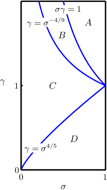
Figure 2: The four parameter regimes given in Theorem 2.1. $A$ is the flat regime, $B$ is the laminate regime, $C$ is the localised branching regime, and $D$ is the uniform branching regime.

Define an additional parameter regime

$$D^{\prime}:=\{(\sigma,{\gamma})\in X:{\gamma}<\sigma^{1/2}\}\supset D.$$

Theorem 2.2 (Lower Bounds).

Let $\gamma\geq 0$, $\sigma\in(0,1)$, $0<l_{1}\leq l_{2}$. There exists a positive constant c, independent of $l_{1}$, $l_{2}$, $\sigma$, and ${\gamma}$, such that for all $(\mathboit u,w)\in V$

(σγ)2/3if σ1/2≤γ≤σ−1,σif γ<σ1/2.(regime D′).I^{(\sigma,\gamma)}[\mathboit u,w]\geq c\,l_{1}l_{2}\left\{\!\!\!\begin{tabular}[]{lll}$1$&if $\gamma\geq\sigma^{-1}$&\text{(regime $A$),}\\ $(\sigma\gamma)^{2/3}$&if $\sigma^{1/2}\leq\gamma\leq\sigma^{-1}$,\\ $\sigma$&if $\gamma<\sigma^{1/2}$.&\text{(regime $D^{\prime}$).}\end{tabular}\right.

(2.2) 1 if ≥γσ-1 (regime A),

Proof.

This follows immediately from Lemma 3.1 and Lemma 3.2 in Section 3 below, using the fact that $(\sigma\gamma)^{2/3}\geq\sigma$ is equivalent to $\gamma\geq\sigma^{1/2}$. ∎

Remark 2.3 (Optimality of the bounds in regimes $A$ and $D$).

The bounds for regimes $A$ and $D$ are optimal in the sense that the lower and upper bounds scale the same way in the parameters $\sigma$ and $\gamma$:

$$\min_{V}I^{(\sigma,{\gamma})}\sim\left\{\begin{array}[]{ll}1&\textrm{if }(\sigma,{\gamma})\in A,\\ \sigma&\textrm{if }(\sigma,\gamma)\in D.\end{array}\right.$$

Proving optimal bounds in the whole parameter space $X$ remains an open problem.

Idea of the proof of Theorem 2.1.

We describe the constructions used to obtain the upper bounds in Theorem 2.1, which correspond to different folding patterns of the thin film. The type of pattern is determined by the competition between the stretching, bending and bonding energies.

In the flat regime $A$ the bonding strength ${\gamma}$ is large compared to $\sigma$ and the upper bound $I^{(\sigma,{\gamma})}\leq c\,l_{1}l_{2}$ is obtained by taking $w=0$ everywhere, i.e., by taking the film to be bonded to the substrate everywhere. See Lemma 4.1. In regimes $B$–$D$, where the bonding strength ${\gamma}$ is smaller, this upper bound can be improved by allowing the film to relax the in-plane compression by partially delaminating from the substrate and buckling.

In the laminate regime $B$ we obtain the upper bound $I^{(\sigma,{\gamma})}\leq c\,l_{1}l_{2}(\sigma{\gamma})^{2/5}$ with a simple periodic folding pattern interpolated to the clamped boundary conditions, as shown in Figure 3. Note that the film is still bonded to the substrate in a large part of the domain. See Proposition 5.3. In regimes $C$ and $D$ a better upper bound can be achieved using a self-similar branching pattern, where the period of the folding pattern decreases towards the clamped boundary.

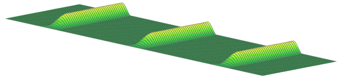
Figure 3: The upper bound construction for the laminate regime $B$. Away from the clamped boundary the film forms a periodic pattern consisting of folds in between regions where it is bonded to the substrate. This is interpolated to the clamped boundary conditions in a thin boundary layer.

In the subset of regime $D$ where $\gamma\leq\sigma$ the bonding energy is a lower order term and the upper bound $I^{(\sigma,{\gamma})}\leq c\,l_{1}l_{2}\sigma$ can be obtained using the same period-halving construction that was used for the case ${\gamma}=0$ in [7], as shown in Figure 4. Note that the film is delaminated from the substrate almost everywhere.

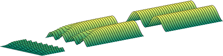
Figure 4: The upper bound construction for parameter regime $\{\gamma\leq\sigma\}\subset D$. Away from the clamped boundary the film forms a periodic folding pattern (right). The folds undergo a sequence of period-halvings (centre) before being interpolated to the clamped boundary (left). The film is delaminated from the substrate almost everywhere, but we do not pay too much bonding energy for this since the bonding strength ${\gamma}$ is small compared to $\sigma$.

In the rest of regime $D$ and in regime $C$ a new upper bound construction is needed. Away from the clamped boundary we take the film to form a periodic pattern, with periodicity cells of the form shown in Figure 5. It is energetically favourable for the period of the pattern to decrease towards the clamped boundary. By construction the stretching energy of each periodicity cell is zero. By requiring that the bending energy of each periodicity cell equals its bonding energy, we find that fold width $2\delta$ is related to the period $2h$ by $\delta\sim h^{1/3}$. Therefore, as we halve the period, $h\mapsto 2^{-1}h$, we must multiply the fold width by a factor of $2^{-1/3}\approx 0.8$. This means that the relative area $\frac{\delta}{h}$ where the film is delaminated in the periodicity cell increases as $h$ decreases. In order to achieve this we perform each period halving $h\mapsto 2^{-1}h$ using a two step refinement procedure consisting of fold shrinkage (Figure 6, right) and fold splitting and separation (Figure 6, left). (For a real film the two branching steps would happen simultaneously, but this does not change the order of the energy.) This takes one cell of period $2h$ and fold width $2\delta$ and produces two cells of period $h$ and fold width $2^{2/3}\delta\approx 1.6\delta$.

We repeat this refinement process until the pattern is fine enough to be interpolated to the clamped boundary conditions without paying too much stretching energy. We will see in the proof of Proposition 6.6 that if $\gamma\geq 1$, then refinement stops before $\delta=h$, i.e., before the film becomes delaminated from the substrate almost everywhere.

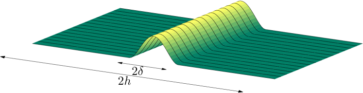
Figure 5: One of the periodicity cells used for regimes $B$, $C$, $D$. A fold of width $2\delta$ lies between two regions where the film is bonded to the substrate.

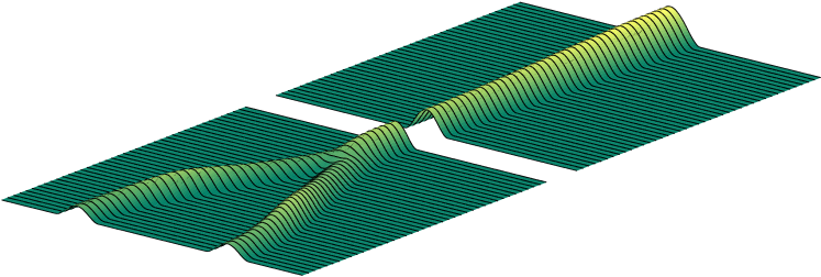
Figure 6: The branching construction used for regimes $C$ and $D$. Each refinement consists of two steps: fold shrinkage (right), where a fold is reduced in width and height, and fold splitting (left), where a fold splits into two folds of the same width.

If $\gamma<1$, however, the pattern refinement continues until $\delta=h$ and the film is delaminated from the substrate almost everywhere. At this point the period of the folds is still too large; if refinement were stopped here then the stretching energy in the interpolation boundary layer would be too high. Therefore we continue refining the pattern towards the clamped boundary by period-halving, $\delta\mapsto 2^{-1}\delta$, using the same construction as for regime $\{\gamma\leq\sigma\}$, shown in Figure 4. This continues until $\delta=l_{1}\sigma$ at which point the pattern is fine enough to be interpolated to the clamped boundary conditions. See the proof of Proposition 6.6.

3 Lower Bound Proofs

In this section we prove the main ingredients of the lower bound in Theorem 2.2.

Lemma 3.1 (Lower bound for $\gamma\geq 0$).

Let $\gamma\geq 0$, $\sigma\in(0,1)$, $0<l_{1}\leq l_{2}$. Then for all $(\mathboit u,w)\in V$

$$I^{(\sigma,{\gamma})}[\mathboit u,w,l_{1},l_{2}]\geq c\,l_{1}l_{2}\sigma.$$

Proof.

By scaling it suffices to consider the case $l_{1}=1$. Further, it suffices to prove the bound for $l_{2}=1$, and apply it to each of the squares $(0,1)\times(k,k+1)$, $k\in\mathbb{N}\cap[0,l_{2}-1]$, and use that $\lfloor l_{2}\rfloor\geq l_{2}/2$ for all $l_{2}\geq 1$.

The bound for $l_{1}=l_{2}=1$ and ${\gamma}=0$ was proven in [7, Lemma 1] and implies the general case ${\gamma}\geq 0$ since $I^{(\sigma,{\gamma})}\geq I^{(\sigma,0)}$. ∎

Lemma 3.2 (Lower bounds for $\gamma\geq\sigma^{2}$).

Let $\sigma\in(0,1]$, $\gamma\geq\sigma^{2}$. Then for all $(\mathboit u,w)\in V$

$$I^{(\sigma,{\gamma})}[\mathboit u,w,l_{1},l_{2}]\geq c\,l_{1}l_{2}\left\{\begin{array}[]{ll}1&\textrm{if }\gamma\geq\sigma^{-1},\\ (\sigma\gamma)^{2/3}&\textrm{if }\sigma^{2}\leq\gamma\leq\sigma^{-1}.\end{array}\right.$$

Proof.

As above, it suffices to consider the case $l_{1}=l_{2}=1$. Let $l\in(0,1]$. Subdivide $\Omega:=(0,1)^{2}$ into $\lceil l^{-1}\rceil^{2}$ squares of side length $l$, denoted by $q_{ij}$:

$$q_{ij}:=l(i,i+1)\times l(j,j+1)\;\cap\;(0,1)^{2},\qquad i,j\in\{0,\ldots,\lceil l^{-1}\rceil-1\}.$$

We say that $q_{ij}$ is good if

$$|\{w=0\}\cap q_{ij}|\geq\frac{l^{2}}{2}.$$

Otherwise $q_{ij}$ is bad. Let $N_{B}$ be the number of bad squares, $\Omega_{G}$ be the union of all the good squares, and $\Omega_{B}$ be the union of the bad ones. Let $E$ be the energy of a given deformation $(\mathboit u,w)$. It is easy to see that

$$N_{B}\frac{l^{2}}{2}\;\leq\;|\Omega_{B}\cap\{w>0\}|\;\leq\;|\{w>0\}|\;\leq\;\frac{E}{\gamma},$$

which implies

(3.1) $$N_{B}\leq\frac{2E}{\gamma l^{2}}.$$

Let $q_{ij}$ be a good square. By the Poincaré inequality

(3.2) $$\int_{q_{ij}}|Dw|^{2}\,d\mathboit x\leq l^{2}\int_{q_{ij}}|D^{2}w|^{2}\,d\mathboit x.$$

(The Poincaré constant $l^{2}$ is obtained in Appendix C.) Summing over all good squares yields

(3.3) $$\int_{\Omega_{G}}|Dw|^{2}\,d\mathboit x\leq l^{2}\int_{\Omega_{G}}|D^{2}w|^{2}\,d\mathboit x\leq\frac{l^{2}}{\sigma^{2}}E.$$

Define

$$\eta:=\int_{\Omega_{G}}|D\mathboit u+D\mathboit u^{T}-\mathrm{Id}|\,d\mathboit x.$$

We claim that

(3.4) $$\eta\leq E^{1/2}+\frac{l^{2}}{\sigma^{2}}E.$$

Proof: First note that

(3.5) $$E\geq\int_{\Omega}|D\mathboit u+D\mathboit u^{T}-\mathrm{Id}+Dw\otimes Dw|^{2}\,d\mathboit x\geq\left(\int_{\Omega}|D\mathboit u+D\mathboit u^{T}-\mathrm{Id}+Dw\otimes Dw|\,d\mathboit x\right)^{2}$$

by the Cauchy-Schwarz inequality since $\Omega$ has area 1. By the definition of the Frobenius norm

$$|Dw\otimes Dw|^{2}=w_{x}^{4}+2w_{x}^{2}w_{y}^{2}+w_{y}^{4}=(w_{x}^{2}+w_{y}^{2})^{2}=|Dw|^{4}.$$

Therefore

(3.6) $$\int_{\Omega_{G}}|Dw\otimes Dw|\,d\mathboit x=\int_{\Omega_{G}}|Dw|^{2}\,d\mathboit x\leq\frac{l^{2}}{\sigma^{2}}E$$

by equation (3.3). Using the triangle inequality and combining (3.5) and (3.6) gives

$$\eta\leq\int_{\Omega_{G}}|D\mathboit u+D\mathboit u^{T}-\mathrm{Id}+Dw\otimes Dw|\,d\mathboit x+\int_{\Omega_{G}}|Dw\otimes Dw|\,d\mathboit x\leq E^{1/2}+\frac{l^{2}}{\sigma^{2}}E$$

as required.

At this point we define $\mathboit U(\mathboit x):=(2\mathboit u(\mathboit x)-\mathboit x)\chi_{\Omega_{G}}(\mathboit x)$. Then $\mathboit U\in SBV(\Omega;\mathbb{R}^{2})\subset SBD(\Omega)$ and its jump set $JU$ is contained in the union of the boundaries of the bad squares, hence $\mathcal{H}^{1}(JU)\leq 4lN_{B}\leq 8E/\gamma l$ by (3.1). At the same time, $\|e(\mathboit U)\|_{L^{1}(\Omega)}=\eta$. By the Korn-Poincaré inequality for $SBD$ functions proven in [12, Th. 1] (with $p=1$) we obtain that there are a set $\omega_{\Gamma}\subset\partial\Omega$ with $\mathcal{H}^{1}(\omega_{\Gamma})\leq c\mathcal{H}^{1}(JU)$ and an affine function $\boldsymbol{a}$ with $D\boldsymbol{a}+D\boldsymbol{a}^{T}=0$ such that $\int_{\{0\}\times(0,1)\setminus\omega_{\Gamma}}|\boldsymbol{a}(\mathboit x)-\mathboit x|d\mathcal{H}^{1}(\mathboit x)\leq c\eta$. Since $a_{2}$ is constant on this set, if the length of $\omega_{\Gamma}$ is less than $1/2$ we obtain $\eta\geq c$ for some universal constant $c$. Conversely, if the length of $\omega_{\Gamma}$ is more than $1/2$ we obtain $1/2\leq c\mathcal{H}^{1}(JU)\leq cE/\gamma l$. Therefore at least one of $E\geq c\gamma l$ and $\eta\geq c$ holds. Recalling (3.4) this gives

(3.7) $$E\geq c\min\left\{\gamma l,1,\frac{\sigma^{2}}{l^{2}}\right\}.$$

We consider different choices of $l$. Equating the second two terms on the right-hand side of (3.7) gives $l=\sigma$ and

$$E\geq c\min\{\sigma\gamma,1\}=c\quad\textrm{if}\quad\sigma\gamma\geq 1.$$

Equating the first and third terms on the right-hand side of (3.7) gives $l=\sigma^{2/3}\gamma^{-1/3}$ and

$$E\geq c\min\{(\sigma\gamma)^{2/3},1\}=c(\sigma\gamma)^{2/3}\quad\textrm{if}\quad\sigma\gamma\leq 1.$$

Since we require that $l\in(0,1]$, then this estimate is only valid if in addition $\sigma^{2/3}\gamma^{-1/3}\leq 1\Longleftrightarrow\gamma\geq\sigma^{2}$. This completes the proof.

In order to make the argument more transparent we also give a self-contained proof, which does not apply the rigidity estimate in [12, Th. 1] but instead makes direct usage of some ideas from its proof, which can be much simplified in the present context.

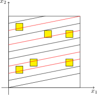
Figure 7: Sketch of the geometry in the proof of Lemma 3.2. The squares in $\Omega_{B}$ are shown, as well as some of the lines $(0,y)+\mathboit n\mathbb{R}$.

We assume for now that

(3.8) $$E\leq\frac{1}{16}\gamma l.$$

Therefore by equations (3.1) and (3.8)

(3.9) $$N_{B}l\leq\frac{1}{8}.$$

Pick $\mathboit n:=(\cos\theta,\sin\theta)\in S^{1}$ with $n_{1}\geq\frac{1}{\sqrt{2}}$, equivalently $\theta\in[-\pi/4,\pi/4]$. Define

$$\omega_{\mathboit n}:=\Big{\{}y\in(0,1)\,:\,\left\{(0,y)+\mathboit n\mathbb{R}\right\}\cap\Omega_{B}=\emptyset\Big{\}},$$

see Figure 7. Note that $\mathcal{L}^{1}(\omega_{\mathboit n}^{c})$ is maximised, e.g., when $\theta=-\pi/4$ and the union of bad squares $\Omega_{B}$ is given by

$$\bigcup_{i=0}^{N_{B}-1}(0,l)\times l(2i,2i+1).$$

In this case each line $(0,y)+\mathboit n\mathbb{R}$ intersects at most one bad square and $\mathcal{L}^{1}(\omega_{\mathboit n}^{c})=2lN_{B}$. By combining this and (3.9) we obtain

$$\mathcal{L}^{1}(\omega_{\mathboit n})\geq 1-2lN_{B}\geq\frac{3}{4}$$

for all admissible $\mathboit n$. For $y\in\omega n$ let $In(y):=\left\{(0,y)+\mathboit n\mathbb{R}\right\}\cap(0,1)^{2}$ and

$$\Omega n:=\bigcup_{y\in\omega n}In(y).$$

We estimate

(3.10) $$\int_{\Omega n}|D\mathboit u+D\mathboit u^{T}-\mathrm{Id}|\,d\mathboit x\leq\int_{\Omega_{G}}|D\mathboit u+D\mathboit u^{T}-\mathrm{Id}|\,dx=\eta.$$

The function $f_{n}(\mathboit x):=2\mathboit n\cdot\mathboit u(\mathboit x)-\frac{x_{1}}{n_{1}}$ vanishes at $x_{1}=0$ since $\mathboit u$ satisfies the boundary condition $\mathboit u(0,y)=(0,0)$. Also

(3.11) $$Dfn\cdot\mathboit n=2\mathboit n\cdot D\mathboit u\cdot\mathboit n-1=\mathboit n\cdot(D\mathboit u+D\mathboit u^{T}-\mathrm{Id})\mathboit n.$$

By the Poincaré inequality, (3.11) and (3.10)

(3.12) $$\int_{\Omega n}|fn|\,d\mathboit x\leq c\int_{\Omega n}|Dfn\cdot\mathboit n|\,d\mathboit x\leq c\int_{\Omega n}|D\mathboit u+D\mathboit u^{T}-Id|\,d\mathboit x\leq c\eta$$

for some $c>0$. Fix three different, admissible values of $\mathboit n$, called $\mathboit n$, $\mathboit n^{\prime}$, $\mathboit n^{\prime\prime}$, with corresponding angles $\theta$, $\theta^{\prime}$, $\theta^{\prime\prime}$. Set $\tilde{\Omega}=\Omega n\cap\Omega_{\mathboit n^{\prime}}\cap\Omega_{\mathboit n^{\prime\prime}}$. Then

$$|\tilde{\Omega}|>\frac{1}{64},$$

where the number on the right-hand side is obtained by taking $\theta=\pi/4$, $\theta^{\prime}=-\pi/4$, $\theta^{\prime\prime}=0$, $\omega n=[1/4,1]$, $\omega_{\mathboit n^{\prime}}=[0,3/4]$, $\omega_{\mathboit n^{\prime\prime}}=[0,3/8]\cup[5/8,1]$.

Given $x_{1}>0$, consider the following over-determined linear system for $\mathboit v\in\mathbb{R}^{2}$:

$$2\mathboit n\cdot\mathboit v=\frac{x_{1}}{n_{1}},\quad 2\mathboit n^{\prime}\cdot\mathboit v=\frac{x_{1}}{n^{\prime}_{1}},\quad 2\mathboit n^{\prime\prime}\cdot\mathboit v=\frac{x_{1}}{n^{\prime\prime}_{1}},$$

which can be written as

(3.13) $$2\begin{pmatrix}\mathboit n\\ \mathboit n^{\prime}\\ \mathboit n^{\prime\prime}\end{pmatrix}\mathboit v=x_{1}\begin{pmatrix}1/n_{1}\\ 1/n_{1}^{\prime}\\ 1/n_{1}^{\prime\prime}\end{pmatrix}$$

if we consider $\mathboit n$, $\mathboit n^{\prime}$, $\mathboit n^{\prime\prime}$ to be row vectors. It is easy to check that the null-space of the adjoint of the matrix on the left-hand side is spanned by $(\sin(\theta^{\prime}-\theta^{\prime\prime}),\sin(\theta^{\prime\prime}-\theta^{\prime}),\sin(\theta-\theta^{\prime}))$. Therefore (3.13) has a solution $\mathboit v$ if and only if

$$0 =\begin{pmatrix}1/n_{1}\\ 1/n_{1}^{\prime}\\ 1/n_{1}^{\prime\prime}\end{pmatrix}\cdot\begin{pmatrix}\sin(\theta^{\prime}-\theta^{\prime\prime})\\ \sin(\theta^{\prime\prime}-\theta^{\prime})\\ \sin(\theta-\theta^{\prime})\end{pmatrix}$$

$$=\frac{1}{2}\big{(}\cos^{2}\theta(\sin 2\theta^{\prime\prime}-\sin 2\theta^{\prime})+\cos^{2}\theta^{\prime}(\sin 2\theta-\sin 2\theta^{\prime\prime})+\cos^{2}\theta^{\prime\prime}(\sin 2\theta^{\prime}-\sin 2\theta)\big{)}.$$

Now choose $\theta>0$, $\theta^{\prime}=-\theta$. Then the right-hand side is nonzero since $\theta^{\prime\prime}\neq\pm\theta$, and there is no solution $\mathboit v$ to (3.13). Therefore for this choice of $\mathboit n$, $\mathboit n^{\prime}$, $\mathboit n^{\prime\prime}$

(3.14) $$\min_{v\in\mathbb{R}^{2}}\left|2\mathboit n\cdot\mathboit v-\frac{x_{1}}{n_{1}}\right|+\left|2\mathboit n^{\prime}\cdot\mathboit v-\frac{x_{1}}{n^{\prime}_{1}}\right|+\left|2\mathboit n^{\prime\prime}\cdot\mathboit v-\frac{x_{1}}{n^{\prime\prime}_{1}}\right|>0$$

for any $x_{1}>0$ and uniformly if $x_{1}\geq x_{1}^{*}>0$. By (3.4), (3.12), (3.14)

$$E^{1/2}+\frac{l^{2}}{\sigma^{2}}E \geq\eta$$

$$\geq\frac{1}{3c}\int_{\tilde{\Omega}\cap\{x_{1}\geq x_{1}^{*}\}}|fn|+|f_{\mathboit n^{\prime}}|+|f_{\mathboit n^{\prime\prime}}|\,d\mathboit x$$

$$\geq\frac{1}{3c}|\tilde{\Omega}\cap\{x_{1}\geq x_{1}^{*}\}|\min_{\begin{subarray}{c}v\in\mathbb{R}^{2}\\ x_{1}\in[x_{1}^{*},1]\end{subarray}}\left|2\mathboit n\cdot\mathboit v-\frac{x_{1}}{n_{1}}\right|+\left|2\mathboit n^{\prime}\cdot\mathboit v-\frac{x_{1}}{n^{\prime}_{1}}\right|+\left|2\mathboit n^{\prime\prime}\cdot\mathboit v-\frac{x_{1}}{n^{\prime\prime}_{1}}\right|$$

(3.15) $$\geq\tilde{c}$$

for some constant $\tilde{c}>0$. Putting together (3.8) and (3.15) leads to (3.7), and the proof is concluded as above. ∎

4 Upper Bound Construction for the Flat Regime $A$

In this section we prove Theorem 2.1 for parameter regime $A$. In this regime ${\gamma}$ is very large and the upper bound is obtain by taking the film to be bonded to the substrate everywhere.

Lemma 4.1 (Energy of the flat construction).

There exists a constant $c>0$ such that for all $\sigma\in(0,1)$, $\gamma>0$

(4.1) $$\min_{V}I^{(\sigma,\gamma)}\leq c\,l_{1}l_{2}.$$

Proof.

The displacement field $(u,v,w)=(0,0,0)$ satisfies the desired upper bound (4.1). Note that a smarter choice of displacement field is $(u,v,w)=(x/2,0,0)$, which yields the same bound (4.1) but with a smaller constant $c$. Here the film relaxes compression in the $x$-direction, the direction orthogonal to the clamped boundary, by spreading out. ∎

5 Upper Bound Construction for the Laminate Regime $B$

In this section we prove Theorem 2.1 for parameter regime $B$. In this regime it is favourable for the film to buckle, but not to exhibit branching patterns. See Figure 3.

In this and the next Section we work in components, so we write $\mathboit x=(x,y)$ and $\mathboit u=(u,v)$, the stretching energy takes the form

(5.1) $$I_{\textrm{S}}=\int_{\Omega}(2u_{x}+w_{x}^{2}-1)^{2}\,d\mathboit x+2\int_{\Omega}(u_{y}+v_{x}+w_{x}w_{y})^{2}\,d\mathboit x+\int_{\Omega}(2v_{y}+w_{y}^{2}-1)^{2}\,d\mathboit x.$$

5.1 Construction in the Interior

First we construct a displacement field on an interior rectangle of $(0,l_{1})\times(0,l_{2})$, away from the clamped boundary $\{x=0\}$. By translation invariance of the energy we can take the rectangle to be $(0,l)\times(-h,h)$ with $l<l_{1}$, $2h\leq l_{2}$. Take $\delta<h$ and consider a vertical displacement of the form

(5.2) $$w(x,y):=w(y):=\left\{\begin{array}[]{cl}0&y\in(-h,-\delta],\\ \displaystyle\frac{A}{2}\left(1+\cos\frac{\pi y}{\delta}\right)&y\in[-\delta,\delta],\\ 0&y\in[\delta,h).\end{array}\right.$$

This describes an $x$-independent displacement where the film has one fold of height $A$ and width $2\delta$, and is bonded down to the substrate elsewhere, see Figure 5. Choosing $u$ and $v$ so that the stretching energy vanishes, i.e., $I_{\mathrm{S}}=0$, and with $v(x,-h)=v(x,h)=0$ yields

(5.3) $$u(x,y) :=u(x):=\frac{1}{2}x+d,$$

$$v(x,y) :=v(y):=\left\{\begin{array}[]{cl}\vskip 3.0pt plus 1.0pt minus 1.0pt\displaystyle\frac{1}{2}(y+h)&y\in(-h,-\delta],\\ \vskip 3.0pt plus 1.0pt minus 1.0pt\displaystyle\frac{y}{2}-\frac{A^{2}\pi^{2}}{16\delta^{2}}\left(y-\frac{\delta}{2\pi}\sin\frac{2\pi y}{\delta}\right)&y\in[-\delta,\delta],\\ \displaystyle\frac{1}{2}(y-h)&y\in[\delta,h),\end{array}\right.$$

for any constant $d$. In order for $v$ to be continuous we must have

(5.4) $$A^{2}=\frac{8}{\pi^{2}}\delta h.$$

It is a simple calculus exercise to verify the following:

Lemma 5.1 (Energy of the basic laminate construction).

The displacement $(u,v,w)$ defined in equations (5.2)–(5.4) has the following energy on the rectangle $(0,l)\times(-h,h)$:

$$I^{(\sigma,\gamma)}=2\pi^{2}(\sigma l_{1})^{2}\frac{lh}{\delta^{2}}+2{\gamma}l\delta.$$

5.2 Construction in the Boundary Layer

We define a displacement field $(\tilde{u},\tilde{v},\tilde{w})$ on a boundary layer rectangle $(0,\varepsilon)\times(-h,h)$ by interpolating between the clamped boundary conditions (1.4) and the displacements introduced in equations (5.2)–(5.4): Let

(5.5) $$\tilde{u}(x):=\frac{1}{2}x,\quad\tilde{v}(x,y):=\psi^{2}\left(\frac{x}{\varepsilon}\right)v(y),\quad\tilde{w}(x,y):=\psi\left(\frac{x}{\varepsilon}\right)w(y),$$

where $\psi$ is the cubic interpolating polynomial satisfying $\psi(0)=0$, $\psi(1)=1$, $\psi^{\prime}(0)=\psi^{\prime}(1)=0$, i.e.,

$$\psi(t):=t^{2}(3-2t).$$

Note that in (5.5) we take $\tilde{v}=\psi^{2}v$ rather than the more natural choice of $\tilde{v}=\psi v$ since then the stretching term $\tilde{w}_{y}^{2}+2\tilde{v}_{y}-1$ is of order $1$ rather than of order $h/\delta$. See equation (5.9).

We extend $(\tilde{u},\tilde{v},\tilde{w})$ to the whole boundary layer $(0,\varepsilon)\times(0,l_{2})$ by gluing together $l_{2}/2h$ copies of $(\tilde{u},\tilde{v},\tilde{w})$ along their horizontal boundaries. (If $2h$ does not divide $l_{2}$, then we glue together $\lfloor l_{2}/2h\rfloor$ copies to get a construction on $(0,\varepsilon)\times(0,2h\lfloor l_{2}/2h\rfloor)$ and define $u=x/2$, $v=w=0$ on $(0,\varepsilon)\times(2h\lfloor l_{2}/2h\rfloor,l_{2})$. For simplicity we assume that $2h$ divides $l_{2}$ in the rest of the paper since it does not affect the energy bound.)

Lemma 5.2 (Energy of the boundary layer construction).

Let $0<\delta\leq\varepsilon$, $\delta\leq h\leq l_{2}$. The displacement field $(\tilde{u},\tilde{v},\tilde{w}):(0,\varepsilon)\times(0,l_{2})\to\mathbb{R}^{3}$ defined above satisfies the following energy bound:

(5.6) $$I^{(\sigma,\gamma)}\leq Cl_{2}\left(\frac{h^{2}}{{\varepsilon}}+{\varepsilon}+(\sigma l_{1})^{2}\frac{{\varepsilon}}{\delta^{2}}+{\gamma}\frac{{\varepsilon}\delta}{h}\right).$$

Proof.

Observe that $w$, defined in equation (5.2), satisfies the following:

$$|\partial^{m}_{y}w|\leq Ch^{1/2}\delta^{1/2-m}\quad\textrm{for }m\geq 0.$$

Thus $\tilde{w}$ satisfies

(5.7) $$|\partial^{n}_{x}\partial^{m}_{y}\tilde{w}|\leq Ch^{1/2}\delta^{1/2-m}\varepsilon^{-n}\quad\textrm{for }m\geq 0,\textrm{ }n\geq 0.$$

The displacement $v$, defined in equation (5.3), satisfies $|v|\leq Ch$ and so

(5.8) $$|\tilde{v}_{x}|\leq C\frac{h}{\varepsilon}.$$

Recall that $v$ was chosen so that $w_{y}^{2}+2v_{y}-1=0$. Therefore

(5.9) $$|\tilde{w}_{y}^{2}+2\tilde{v}_{y}-1|=|\psi^{2}(w_{y}^{2}+2v_{y}-1)-(1-\psi^{2})|=|1-\psi^{2}|\leq 1.$$

From equations (5.7)–(5.9) we can estimate the stretching, bending, and bonding energy in the boundary layer $(0,\varepsilon)\times(0,l_{2})$:

(5.10) $$I_{\textrm{S}}\leq Cl_{2}\left[\frac{h\delta^{3}}{\varepsilon^{3}}+\frac{h^{2}}{\varepsilon}+\varepsilon\right],\quad I_{\textrm{Be}}\leq C\frac{l_{2}}{h}(\sigma l_{1})^{2}\varepsilon\delta\left[\frac{h\delta}{\varepsilon^{4}}+\frac{h}{\delta\varepsilon^{2}}+\frac{h}{\delta^{3}}\right],\quad I_{\textrm{Bo}}\leq C\frac{l_{2}}{h}{\gamma}\varepsilon\delta.$$

By using the assumptions $\delta\leq{\varepsilon}$ and $\delta\leq h$, the bounds (5.10) reduce to (5.6), as required. ∎

5.3 Complete Construction

We are now in a position to prove the upper bound for the laminate regime $B$:

Proposition 5.3 (Energy of the laminate construction).

Let $0<l_{1}\leq l_{2}$, $\sigma{\gamma}\leq 1$, ${\gamma}\geq 1$. Then

$$\min_{V}I^{(\sigma,\gamma)}\leq Cl_{1}l_{2}(\sigma{\gamma})^{2/5}.$$

Proof.

Take the displacement field $(u,v,w)$ that was defined in (5.2)–(5.4) on $(0,l)\times(-h,h)$ and extend it to the domain $(\varepsilon,l_{1})\times(0,l_{2})$ by taking $l=l_{1}-\varepsilon$, $d={\varepsilon}/2$, and gluing together $l_{2}/2h$ copies along their horizontal boundaries (assuming without loss of generality that $2h$ divides $l_{2}$ as above). Lemma 5.1 implies that this construction has energy

(5.11) $$I^{(\sigma,{\gamma})}\leq C\frac{(l_{1}-{\varepsilon})l_{2}}{h}\left[(\sigma l_{1})^{2}\frac{h}{\delta^{2}}+{\gamma}\delta\right].$$

Define $(u,v,w)$ on $(0,\varepsilon)\times(0,l_{2})$ using the boundary layer construction from Section 5.2. By combining (5.6) and (5.11) we find that the energy on the whole domain $(0,l_{1})\times(0,l_{2})$ satisfies

(5.12) $$I^{(\sigma,{\gamma})} \leq Cl_{2}\left[\frac{h^{2}}{{\varepsilon}}+{\varepsilon}+(\sigma l_{1})^{2}\frac{{\varepsilon}}{\delta^{2}}+{\gamma}\frac{{\varepsilon}\delta}{h}+(\sigma l_{1})^{2}\frac{(l_{1}-{\varepsilon})}{\delta^{2}}+{\gamma}\frac{(l_{1}-{\varepsilon})\delta}{h}\right]$$

$$=Cl_{2}\left[\frac{h^{2}}{{\varepsilon}}+{\varepsilon}+(\sigma l_{1})^{2}\frac{l_{1}}{\delta^{2}}+{\gamma}\frac{l_{1}\delta}{h}\right].$$

Now we chose ${\varepsilon}$, $h$, and $\delta$ to minimise the order of the energy. This can be done by equating terms on the right-hand side of (5.12), which yields

(5.13) $$h=l_{1}(\sigma{\gamma})^{2/5},\quad{\varepsilon}=h,\quad\delta=(\sigma l_{1})^{2/3}{\gamma}^{-1/3}h^{1/3}=l_{1}\sigma^{4/5}{\gamma}^{-1/5}.$$

Note that the conditions $l_{1}\leq l_{2}$, $\sigma{\gamma}\leq 1$, ${\gamma}\geq 1$ ensure that the geometrical restrictions $\delta\leq h$, $h\leq l_{2}$, ${\varepsilon}\leq l_{1}$ and the constraint $\delta\leq{\varepsilon}$ are satisfied. Substituting (5.13) into (5.12) gives

$$I^{(\sigma,{\gamma})}\leq l_{1}l_{2}(\sigma{\gamma})^{2/5}$$

as required. ∎

6 Upper Bound Constructions for the Branching Regimes $C$ and $D$

In this section we prove Theorem 2.1 for the branching regimes $C$ and $D$. The basic idea is to use copies of a folding pattern of the form shown in Figure 5 and to decrease $h$ and $\delta$ towards the clamped boundary by a sequence of fold branchings.

6.1 Branching constructions.

First we prove a general lemma about the cost of fold branching. This covers both our fold splitting construction (Lemma 6.3) and our fold shrinkage construction (Lemma 6.4).

Lemma 6.1 (The cost of branching).

Let $\Omega=(0,l)\times(-h,h)$, $h\leq l$. Let $0<\delta\leq h$ and let $w\in C^{4}(\Omega;[0,\infty))$ satisfy the following:

• $w(x,y)=0$ for $y$ in a neighbourhood of $\pm h$; $w_{x}(x,y)=0$ for $x$ in a neighbourhood of $0$, $l$;

• $w(x,-y)=w(x,y)$;

• For all $x\in(0,l)$

  $$\int_{0}^{h}(1-w_{y}^{2})\,dy=0;$$

• For all $a,b\in\{0,1,2\}$,

  (6.1) $$|\partial^{a}_{x}\partial^{b}_{y}w|\leq c\left(\frac{h}{\delta l}\right)^{a}\left(\frac{1}{\delta}\right)^{b}(h\delta)^{1/2}.$$

Define

(6.2) $$v(x,y):=\frac{1}{2}\int_{-h}^{y}(1-w_{y}^{2})\,d\tilde{y},\qquad u(x,y):=\frac{1}{2}x-\int_{-h}^{y}(w_{x}w_{y}+v_{x})\,d\tilde{y}.$$

Then $v=0$ for $y=\pm h$ and $u=\frac{1}{2}x$ on $\partial\Omega$, and $v(x,-y)=-v(x,y)$.

Assume additionally either

• $w(x,y)=0$ whenever $|y|>c\delta$

or

• $\delta\leq h/2$ and $w(x,y)=A(x)[\psi_{\delta}(y+\varphi(x))+\psi_{\delta}(y-\varphi(x))]$, where $\psi_{\delta}$ is an even function supported on the interval $[-\delta,\delta]$ satisfying $|\psi_{\delta}^{(k)}|\leq C/\delta^{k}$ for $k\in\{0,1,2\}$, and where $\varphi:[0,l]\to[0,h/2]$ and $|\varphi^{(k)}|\leq Ch/l^{k}$ for $k\in\{0,1,2\}$.

Then

(6.3) $$I^{(\sigma,\gamma)}[\mathboit u,w,\Omega]\leq c\gamma\delta l+c(\sigma l_{1})^{2}\frac{lh}{\delta^{2}}+c\frac{h^{6}}{\delta l^{3}}\,.$$

Remark 6.2 (Assumptions of Lemma 6.1).

Recall that the stretching energy of the film was given in (5.1). The definition of $u$ in (6.2) ensures that the second term of the stretching energy vanishes, and the definition of $v$ ensures that the third term vanishes.

Proof.

First we prove the boundary conditions on $v$. The condition $v(x,-h)=0$ is clear from the definition of $v$. Assumptions (ii) and (iii) imply

(6.4) $$\int_{-h}^{h}(1-w_{y}^{2})\,dy=0$$

hence$v(x,h)=0$. Further, by (ii) we get $v(x,0)=0$. Differentiating (6.4) with respect to $x$ gives

(6.5) $$\int_{-h}^{h}w_{y}w_{xy}\,dy=0.$$

Next we show that $v$ is odd in $y$: By assumption (ii) and equation (6.4)

$$v(x,-y) =\frac{1}{2}\int_{-h}^{-y}1-w_{y}^{2}(x,\tilde{y})\,d\tilde{y}=\frac{1}{2}\int_{y}^{h}1-w_{y}^{2}(x,\tilde{y})\,d\tilde{y}$$

$$=\frac{1}{2}\int_{-h}^{h}1-w_{y}^{2}(x,\tilde{y})\,d\tilde{y}-\frac{1}{2}\int_{-h}^{y}1-w_{y}^{2}(x,\tilde{y})\,d\tilde{y}$$

$$=-v(x,y)$$

as required.

Now we turn to the boundary conditions on $u$. Clearly $u=\frac{1}{2}x$ for $y=-h$ by the definition of $u$. Note that, by (ii), $w_{x}w_{y}$ is an odd function of $y$. Therefore

(6.6) $$\int_{-h}^{h}w_{x}w_{y}\,dy=0.$$

Since $v$ is an odd function of $y$, so is $v_{x}$, and

(6.7) $$\int_{-h}^{h}v_{x}\,dy=0.$$

For future use we differentiate this equation with respect to $x$ and record that

(6.8) $$\int_{-h}^{h}v_{xx}\,dy=0.$$

By equations (6.2)₂, (6.6), (6.7)

$$u(x,h)=\frac{1}{2}x-\int_{-h}^{h}(w_{x}w_{y}+v_{x})\,d\tilde{y}=\frac{1}{2}x.$$

It remains to show that $u=\frac{1}{2}x$ for $x=0,l$. This follows immediately from the definition of $u$ and $v$ and the fact that $w_{x}$ is zero close to $x=0,l$ (assumption (i)).

Now we compute the energy bound (6.3). It is easy to see that the bonding energy $I_{\textrm{Bo}}:=\gamma|\{(x,y)\in\Omega:w(x,y)>0\}|$ satisfies $I_{\textrm{Bo}}\leq c\gamma\delta l$ in both cases (v) and (vi), which gives the first term in equation (6.3).

To estimate the bending energy we observe that by (iv) and the assumption $h\leq l$

$$|D^{2}w|^{2}=w_{xx}^{2}+2w_{xy}^{2}+w_{yy}^{2}\leq ch\delta\left(\left(\frac{h}{\delta l}\right)^{4}+2\left(\frac{h}{\delta l}\right)^{2}\left(\frac{1}{\delta}\right)^{2}+\left(\frac{1}{\delta}\right)^{4}\right)\leq c\frac{h\delta}{\delta^{4}}=c\frac{h}{\delta^{3}}.$$

Therefore in both cases (v) and (vi) the bending energy satisfies

(6.9) $$(\sigma l_{1})^{2}\int_{\Omega}|D^{2}w|^{2}\,d\mathboit x\leq c(\sigma l_{1})^{2}\delta l\frac{h}{\delta^{3}}=c(\sigma l_{1})^{2}\frac{lh}{\delta^{2}},$$

which gives the second term in equation (6.3).

Now we come to the stretching energy. By the definition of $u$ and $v$ we only need to estimate

$$I_{\textrm{S}}=\int_{\Omega}(2u_{x}+w_{x}^{2}-1)^{2}\,d\mathboit x$$

(see Remark 6.2). From the definition of $u$, equation (6.8), and the fact that $w_{y}w_{xx}$ is an odd function of $y$ (assumption (ii)), we compute

(6.10) $$u_{x}=\frac{1}{2}-\int_{-h}^{y}(w_{xy}w_{x}+w_{y}w_{xx}+v_{xx})\,d\tilde{y}=\frac{1}{2}+\int_{y}^{h}(w_{xy}w_{x}+w_{y}w_{xx}+v_{xx})\,d\tilde{y}.$$

From the definition of $v$ and equation (6.5) we see that

(6.11) $$v_{x}=-\int_{-h}^{y}w_{y}w_{xy}\,d\tilde{y}=\int_{y}^{h}w_{y}w_{xy}\,d\tilde{y}$$

and therefore

(6.12) $$v_{xx}=-\int_{-h}^{y}w_{xy}^{2}+w_{y}w_{xxy}\,d\tilde{y}=\int_{y}^{h}w_{xy}^{2}+w_{y}w_{xxy}\,d\tilde{y}.$$

By assumption (iv)

(6.13) $$|w_{xy}w_{x}+w_{y}w_{xx}|\leq\left(\frac{h}{\delta l}\right)\left(\frac{1}{\delta}\right)(h\delta)^{1/2}\left(\frac{h}{\delta l}\right)(h\delta)^{1/2}+\left(\frac{1}{\delta}\right)(h\delta)^{1/2}\left(\frac{h}{\delta l}\right)^{2}(h\delta)^{1/2}\leq c\frac{h^{3}}{\delta^{2}l^{2}}.$$

First we consider case (v). Since $w=0$ for $|y|\geq\delta$, then from equations (6.10) and (6.12) we see that $u_{x}=\frac{1}{2}$ for $|y|\geq\delta$. Therefore the stretching energy reduces to

(6.14) $$I_{\textrm{S}}=\int_{0}^{l}\int_{-\delta}^{\delta}(2u_{x}+w_{x}^{2}-1)^{2}\,dydx.$$

For $|y|<\delta$ equations (6.10), (6.12) reduce to

(6.15) $$u_{x}=\frac{1}{2}-\int_{-\delta}^{y}w_{xy}w_{x}+w_{y}w_{xx}+v_{xx}\,d\tilde{y}=\frac{1}{2}+\int_{y}^{\delta}w_{xy}w_{x}+w_{y}w_{xx}+v_{xx}\,d\tilde{y},$$

(6.16) $$v_{xx}=-\int_{-\delta}^{y}w_{xy}^{2}+w_{y}w_{xxy}\,d\tilde{y}=\int_{y}^{\delta}w_{xy}^{2}+w_{y}w_{xxy}\,d\tilde{y}.$$

By equation (6.16) and assumption (iv)

(6.17) $$|v_{xx}|\leq c\delta\left(\left(\frac{h}{\delta l}\right)^{2}\left(\frac{1}{\delta}\right)^{2}h\delta+\frac{(h\delta)^{1/2}}{\delta}\left(\left(\frac{h}{\delta l}\right)^{2}\left(\frac{1}{\delta}\right)(h\delta)^{1/2}\right)\right)\leq c\frac{h^{3}}{\delta^{2}l^{2}}.$$

Using (6.15), (6.13), (6.17) we estimate

(6.18) $$|2u_{x}-1|\leq c\delta\left(\frac{h^{3}}{\delta^{2}l^{2}}+\frac{h^{3}}{\delta^{2}l^{2}}\right)\leq c\frac{h^{3}}{\delta l^{2}}.$$

We conclude from equation (6.14), (6.18) and assumption (iv) that

(6.19) $$I_{\textrm{S}}\leq 2\int_{0}^{l}\int_{-\delta}^{\delta}|2u_{x}-1|^{2}+|w_{x}|^{4}\,dydx\leq cl\delta\frac{h^{6}}{\delta^{2}l^{4}}=c\frac{h^{6}}{\delta l^{3}}.$$

This gives the third term in equation (6.3) and completes the proof for case (v).

We finish by computing the stretching energy for case (vi). We decompose $\Omega$ as $\Omega=\Omega_{1}\cup\Omega_{2}\cup\Omega_{3}$ where

$$\Omega_{1} :=\{(x,y)\in\Omega:\delta-\varphi(x)<y<-\delta+\varphi(x)\},$$

$$\Omega_{2} :=\{(x,y)\in\Omega:-\delta+\varphi(x)\leq y\leq\delta+\varphi(x)\}\cup\{(x,y)\in\Omega:-\delta-\varphi(x)\leq y\leq\delta-\varphi(x)\},$$

$$\Omega_{3} :=\{(x,y)\in\Omega:y>\delta+\varphi(x)\}\cup\{(x,y)\in\Omega:y<-\delta-\varphi(x)\}.$$

Observe that $w=0$ in $\Omega_{1}$ and $\Omega_{3}$. $\Omega_{1}$ is the central region between the two folds, which occupy region $\Omega_{2}$. The same arguments used in the proof of case (v) show that the stretching energy in region $\Omega_{3}$ is zero and that the stretching energy in region $\Omega_{2}$ satisfies estimate (6.19). (The integral over $(-\delta,\delta)$ in (6.19) is replaced with integrals over $(-\delta-\varphi(x),\delta-\varphi(x))$ and $(-\delta+\varphi(x),\delta+\varphi(x))$.) It remains to compute the stretching energy in the central region $\Omega_{1}$. Since $w=0$ in this region we only need to estimate

$$\int_{\Omega_{1}}|2u_{x}-1|^{2}\,dxdy.$$

First we show that $v_{x}=0$ in $\Omega_{1}$. We only need to consider values of $x$ such that $\varphi(x)>\delta$. Since $w=0$ in $\Omega_{1}$ and $\Omega_{3}$, equation (6.11) reduces to the following in $\Omega_{1}$:

(6.20) $$v_{x}=-\int_{-\varphi(x)-\delta}^{-\varphi(x)+\delta}w_{y}w_{xy}\,d\tilde{y}=\int_{\varphi(x)-\delta}^{\varphi(x)+\delta}w_{y}w_{xy}\,d\tilde{y}\qquad\textrm{in }\Omega_{1}.$$

But $w_{y}w_{xy}$ is even in $y$. Therefore

(6.21) $$\int_{\varphi(x)-\delta}^{\varphi(x)+\delta}w_{y}w_{xy}\,d\tilde{y}=\int_{-\varphi(x)-\delta}^{-\varphi(x)+\delta}w_{y}w_{xy}\,d\tilde{y}.$$

Combining (6.20) and (6.21) proves that $v_{x}=0$ in $\Omega_{1}$, as claimed. Recalling (6.2), it follows that

$$u_{y}=-w_{x}w_{y}-v_{x}=0\qquad\textrm{in }\Omega_{1}.$$

Therefore $u(x,y)=u(x,0)$ for all $(x,y)\in\Omega_{1}$. Using assumption (vi) we compute, for $y<0$,

$$w_{x} =A^{\prime}(x)\psi_{\delta}(y+\varphi(x))+A(x)\varphi^{\prime}(x)\psi^{\prime}_{\delta}(y+\varphi(x)),$$

$$w_{y} =A(x)\psi^{\prime}_{\delta}(y+\varphi(x))$$

(since $(x,y)\in\Omega_{1}$, we have $\varphi(x)\geq\delta$). It follows that, again for $y<0$,

$$w_{x}w_{y}=A(x)A^{\prime}(x)\frac{1}{2}\frac{d}{dy}\psi_{\delta}^{2}(y+\varphi(x))+w_{y}^{2}(x,y)\varphi^{\prime}(x).$$

Integrating gives

$$\int_{-h}^{0}w_{x}w_{y}\,dy= =\frac{1}{2}A(x)A^{\prime}(x)\{\psi_{\delta}^{2}(\varphi(x))-\psi_{\delta}^{2}(-h+\varphi(x))\}+\varphi^{\prime}(x)\int_{-h}^{0}w_{y}^{2}\,dy$$

$$=\frac{1}{2}A(x)A^{\prime}(x)\psi_{\delta}^{2}(\varphi(x))+\varphi^{\prime}(x)h$$

by assumption (iii) and since $\varphi(x)\in[0,h/2]$, $\delta<h/2$, and $\psi_{\delta}$ is supported on $[-\delta,\delta]$. Therefore

$$2u(x,0)-x=-2\int_{-h}^{0}(w_{x}w_{y}+v_{x})\,dy=-A(x)A^{\prime}(x)\psi_{\delta}^{2}(\varphi(x))-2h\varphi^{\prime}(x)-2\int_{-h}^{0}v_{x}\,dy.$$

If $(x,0)\in\Omega_{1}$, then $\varphi(x)>\delta$ and so $\psi_{\delta}(\varphi(x))=0$. Hence

$$2u(x,y)-x=2u(x,0)-x=-2h\varphi^{\prime}(x)-2\frac{\partial}{\partial x}\int_{-h}^{0}v\,dy\quad\textrm{ for all }(x,y)\in\Omega_{1}.$$

We compute the integral on the right-hand side:

$$-2\frac{\partial}{\partial x}\int_{-h}^{0}v\,dy=\frac{\partial}{\partial x}\int_{-h}^{0}\int_{-h}^{y}w_{y}^{2}(x,\tilde{y})\,d\tilde{y}\,dy=\frac{\partial}{\partial x}\int_{-h}^{0}\int_{\tilde{y}}^{0}w_{y}^{2}(x,\tilde{y})\,dy\,d\tilde{y}$$

by changing the order of integration. Therefore

$$-2\frac{\partial}{\partial x}\int_{-h}^{0}v\,dy=-\frac{\partial}{\partial x}\int_{-h}^{0}\tilde{y}w_{y}^{2}(x,\tilde{y})\,d\tilde{y}=\frac{\partial}{\partial x}\int_{0}^{h}yw_{y}^{2}(x,y)\,dy.$$

If $(x,0)\in\Omega_{1}$, then

$$-2\frac{\partial}{\partial x}\int_{-h}^{0}v\,dy =\frac{\partial}{\partial x}\int_{\varphi(x)-\delta}^{\varphi(x)+\delta}yw_{y}^{2}(x,y)\,dy$$

$$=\frac{\partial}{\partial x}\int_{\varphi(x)-\delta}^{\varphi(x)+\delta}(y-\varphi(x))w_{y}^{2}(x,y)\,dy+h\varphi^{\prime}(x)\qquad\textrm{(by assumption (iii))}$$

$$=\frac{\partial}{\partial x}\int_{\varphi(x)-\delta}^{\varphi(x)+\delta}(y-\varphi(x))A^{2}(x)[\psi^{\prime}_{\delta}(y-\varphi(x))]^{2}\,dy+h\varphi^{\prime}(x)$$

$$=\frac{\partial}{\partial x}\int_{-\delta}^{\delta}yA^{2}(x)[\psi^{\prime}_{\delta}(y)]^{2}\,dy+h\varphi^{\prime}(x)\qquad\textrm{(by changing variables)}$$

$$=2A(x)A^{\prime}(x)\int_{-\delta}^{\delta}y[\psi^{\prime}_{\delta}(y)]^{2}\,dy+h\varphi^{\prime}(x)$$

$$=h\varphi^{\prime}(x)$$

since $y[\psi^{\prime}_{\delta}(y)]^{2}$ is odd. Therefore, if $(x,y)\in\Omega_{1}$,

$$2u(x,y)-x=-h\varphi^{\prime}(x).$$

We conclude that

$$\int_{\Omega_{1}}|2u_{x}-1|^{2}\,dxdy=\int_{\Omega_{1}}h^{2}|\varphi^{\prime\prime}(x)|^{2}\,dxdy\leq Chl\,h^{2}(h/l^{2})^{2}=C\frac{h^{5}}{l^{3}}\leq C\frac{h^{6}}{\delta l^{3}}$$

since $\delta<h$. Therefore the stretching energy in region $\Omega_{1}$ is the same order (or less) than the stretching energy in region $\Omega_{2}$ and we have finally arrived at the desired estimate (6.3). ∎

In the follow lemma we construct a deformation that takes one fold of width $2\delta$ at $x=l$ and splits it into two folds of width $2\delta$ separated by a distance of $h-2\delta$ at $x=0$. The film is bonded to the substrate between the two folds. See Figure 6, left.

Lemma 6.3 (Fold splitting construction).

Let $0<\delta\leq h/2$. Let $\psi\in C^{\infty}_{c}((-1,1);[0,1])$ be an even function with $\psi(0)=1$. Define $\psi_{\delta}(y)=\psi(y/\delta)$. Let $\varphi\in C^{\infty}([0,l];[0,h/2])$ satisfy $\varphi(0)=h/2$, $\varphi(l)=0$, $\varphi^{\prime}=\varphi^{\prime\prime}=0$ in a neighbourhood of $x=0,l$, and $|\varphi^{(k)}|\leq Ch/l^{k}$ for $k\in\{0,1,2\}$. Set

$$\tilde{w}(x,y):=\psi_{\delta}(y+\varphi(x))+\psi_{\delta}(y-\varphi(x)).$$

Define $A:[0,l]\to(0,\infty)$ by

(6.22) $$A^{2}(x)\int_{0}^{h}\tilde{w}_{y}^{2}(x,y)\,dy=h.$$

Then $w:[0,l]\times[-h,h]\to[0,\infty)$ defined by

(6.23) $$w(x,y):=A(x)\tilde{w}(x,y)$$

satisfies the assumptions of Lemma 6.1.

Proof.

Observe that $w$ satisfies assumption (ii) of Lemma 6.1 since $\psi_{\delta}$ is even. Equation (6.22) ensures that $w$ satisfies assumption (iii). Clearly $w$ also satisfies assumption (vi). It remains to check assumptions (i) and (iv).

Since $\delta\leq h/2$ and $|\varphi|\leq h/2$, then $w(x,y)=0$ for $y$ in a neighbourhood of $\pm h$. We differentiate (6.22) with respect to $x$ and rearrange to get

(6.24) $$A^{\prime}(x)=\frac{\displaystyle-A(x)\int_{0}^{h}\tilde{w}_{y}\tilde{w}_{xy}\,dy}{\displaystyle\int_{0}^{h}\tilde{w}_{y}^{2}\,dy}.$$

By assumption $\varphi^{\prime}$ vanishes in a neighbourhood of $x=0,l$, and consequently so do $\tilde{w}_{xy}$, $A^{\prime}$ and

$$w_{x}(x,y)=A^{\prime}(x)\tilde{w}(x,y)+A(x)(\psi^{\prime}_{\delta}(y+\varphi(x))+\psi^{\prime}_{\delta}(y-\varphi(x)))\varphi^{\prime}(x).$$

Therefore assumption (i) of Lemma 6.1 is satisfied.

Finally we check assumption (iv). Observe that

$$\int_{0}^{h}\tilde{w}_{y}^{2}(x,y)\,dy\geq\int_{\varphi(x)}^{\varphi(x)+\delta}\tilde{w}_{y}^{2}(x,y)\,dy\geq\frac{1}{\delta}\left(\int_{\varphi(x)}^{\varphi(x)+\delta}\tilde{w}_{y}(x,y)\,dy\right)^{2}=\frac{1}{\delta}\tilde{w}^{2}(x,\varphi(x))\geq\frac{1}{\delta}$$

since $\psi(0)=1$. Observing that by definition $|\tilde{w}_{y}|\leq C/\delta$ we conclude

(6.25) $$\frac{1}{\delta}\leq\int_{0}^{h}\tilde{w}_{y}^{2}\,dy\leq\frac{C}{\delta}\qquad\textrm{ and }\qquad c(h\delta)^{1/2}\leq A\leq C(h\delta)^{1/2}.$$

Since $|\tilde{w}_{y}|\leq C\delta^{-1}$ and $|\tilde{w}_{xy}|\leq C|\varphi^{\prime}|\delta^{-2}$, then (6.24) and (6.25) give

$$|A^{\prime}|=|A|\left|\int_{\max\{0,-\delta+\varphi(x)\}}^{\delta+\varphi(x)}\tilde{w}_{y}\tilde{w}_{xy}\,dy\right|\;\left|\int_{0}^{h}\tilde{w}_{y}^{2}\,dy\right|^{-1}\leq C\frac{|A||\varphi^{\prime}|}{\delta}\leq C|A|\frac{h}{\delta l}.$$

Note that

$$|\tilde{w}_{xxy}| \leq|\psi^{\prime\prime\prime}_{\delta}(y+\varphi(x))+\psi^{\prime\prime\prime}_{\delta}(y-\varphi(x))||\varphi^{\prime}|^{2}+|\psi^{\prime\prime}_{\delta}(y+\varphi(x))+\psi^{\prime\prime}_{\delta}(y-\varphi(x))||\varphi^{\prime\prime}|$$

$$\leq C\frac{1}{\delta^{3}}\left(\frac{h}{l}\right)^{2}+C\frac{1}{\delta^{2}}\frac{h}{l^{2}}\leq C\frac{h^{2}}{\delta^{3}l^{2}}$$

since $\delta<h$. Therefore

$$|A^{\prime\prime}| \leq\frac{\displaystyle\left|-A^{\prime}\int_{0}^{h}\tilde{w}_{y}\tilde{w}_{xy}\,dy-A\int_{0}^{h}(\tilde{w}_{xy}^{2}+\tilde{w}_{y}\tilde{w}_{xxy})\,dy\right|}{\displaystyle\int_{0}^{h}\tilde{w}_{y}^{2}\,dy}+2|A|\frac{\displaystyle\left(\int_{0}^{h}\tilde{w}_{y}\tilde{w}_{xy}\,dy\right)^{2}}{\displaystyle\left(\int_{0}^{h}\tilde{w}_{y}^{2}\,dy\right)^{2}}$$

$$\leq C\delta\left(|A^{\prime}|\delta\delta^{-1}|\varphi^{\prime}|\delta^{-2}+|A|\delta(|\varphi^{\prime}|^{2}\delta^{-4}+\delta^{-1}h^{2}\delta^{-3}l^{-2})\right)+C|A|\delta^{2}\left(\delta\delta^{-1}|\varphi^{\prime}|\delta^{-2}\right)^{2}$$

$$\leq C|A|\left(\frac{h}{\delta l}\right)^{2}$$

since $|A^{\prime}|\leq C|A||\varphi^{\prime}|/\delta$ and $|\varphi^{\prime}|\leq Ch/l$. Putting everything together gives

$$|w| \leq|A||\tilde{w}|\leq C(h\delta)^{1/2},$$

$$|w_{x}| \leq|A^{\prime}||\tilde{w}|+|A||\psi^{\prime}_{\delta}(y+\varphi(x))+\psi^{\prime}_{\delta}(y-\varphi(x))||\varphi^{\prime}|\leq C|A||\varphi^{\prime}|\delta^{-1}\leq C(h\delta)^{1/2}\frac{h}{\delta l},$$

$$|w_{y}| \leq|A||\psi^{\prime}_{\delta}(y+\varphi(x))+\psi^{\prime}_{\delta}(y-\varphi(x))|\leq C(h\delta)^{1/2}\frac{1}{\delta},$$

$$|w_{xx}| \leq|A^{\prime\prime}||\tilde{w}|+2|A^{\prime}||\psi^{\prime}_{\delta}(y+\varphi(x))+\psi^{\prime}_{\delta}(y-\varphi(x))||\varphi^{\prime}|+|A||\psi^{\prime\prime}_{\delta}(y+\varphi(x))+\psi^{\prime\prime}_{\delta}(y-\varphi(x))||\varphi^{\prime}|^{2}$$

$$\quad+|A||\psi^{\prime}_{\delta}(y+\varphi(x))+\psi^{\prime}_{\delta}(y-\varphi(x))||\varphi^{\prime\prime}|$$

$$\leq C(h\delta)^{1/2}\left(\frac{h^{2}}{\delta^{2}l^{2}}+\frac{h}{\delta l^{2}}\right)\leq C(h\delta)^{1/2}\left(\frac{h}{\delta l}\right)^{2},$$

$$|w_{xy}| \leq|A^{\prime}||\psi^{\prime}_{\delta}(y+\varphi(x))+\psi^{\prime}_{\delta}(y-\varphi(x))|+|A||\psi^{\prime\prime}_{\delta}(y+\varphi(x))+\psi^{\prime\prime}_{\delta}(y-\varphi(x))||\varphi^{\prime}|$$

$$\leq C(h\delta)^{1/2}\left(\frac{h}{\delta l}\right)\left(\frac{1}{\delta}\right),$$

$$|w_{yy}| \leq|A||\psi^{\prime\prime}_{\delta}(y+\varphi(x))+\psi^{\prime\prime}_{\delta}(y-\varphi(x))|\leq C(h\delta)^{1/2}\left(\frac{1}{\delta}\right)^{2}$$

and hence $w$ satisfies assumption (iv) of Lemma 6.1. ∎

In the following lemma we construct a deformation that takes one fold of width $2\delta$ at $x=l$ and shrinks it down to a fold of width $2\tilde{\delta}<2\delta$ at $x=0$. See Figure 6, right.

Lemma 6.4 (Fold shrinkage construction).

Let $0<\delta\leq h$, $\lambda\in[1/4,1]$. Let $\psi\in C^{\infty}_{c}((-1,1);[0,1])$ be an even function with $\psi(0)=1$. Define $\psi_{\delta}(y):=\psi(y/\delta)$. Let $\hat{\delta}\in C^{2}([0,l];[\lambda\delta,\delta])$ satisfy $\hat{\delta}(0)=\lambda{\delta}$, $\hat{\delta}(l)=\delta$, $\hat{\delta}^{\prime}=0$ in a neighbourhood of $x=0,l$, and $|\hat{\delta}^{(k)}|\leq C\delta/l^{k}$. Set $\tilde{w}(x,y):=\psi_{\hat{\delta}(x)}(y)$. Define $A:[0,l]\to(0,\infty)$ by

(6.26) $$A^{2}(x)\int_{0}^{h}\tilde{w}_{y}^{2}(x,y)\,dy=h.$$

Then $w:[0,l]\times[-h,h]\to[0,\infty)$ defined by

(6.27) $$w(x,y):=A(x)\tilde{w}(x,y)$$

satisfies the assumptions of Lemma 6.1.

Proof.

The same arguments used in the proof of Lemma 6.3 show that $w$ satisfies assumptions (i)–(iii) of Lemma 6.1. Clearly it also satisfies assumption (v). It remains to check assumption (iv). Observe that

$$\int_{0}^{h}\tilde{w}_{y}^{2}(x,y)\,dy=\int_{0}^{h}[\psi_{\hat{\delta}(x)}^{\prime}(y)]^{2}\,dy=\frac{1}{\hat{\delta}^{2}(x)}\int_{0}^{\hat{\delta}(x)}\left[\psi^{\prime}\left(\tfrac{y}{\hat{\delta}(x)}\right)\right]^{2}\,dy=\frac{1}{\hat{\delta}(x)}\int_{0}^{1}[\psi^{\prime}(y)]^{2}\,dy=\frac{c_{*}}{\hat{\delta}(x)}.$$

Therefore

$$A(x)=\left(\frac{\hat{\delta}(x)h}{c_{*}}\right)^{1/2}\leq c(\delta h)^{1/2}.$$

Note that

$$\frac{\partial}{\partial\delta}\psi_{\delta}(y)=-\psi^{\prime}\left(\frac{y}{\delta}\right)\frac{y}{\delta^{2}}.$$

Since $\hat{\delta}(x)\geq\lambda\delta$, we estimate

$$|\tilde{w}_{x}(x,y)| =\left|\psi^{\prime}\left(\frac{y}{\hat{\delta}(x)}\right)\frac{y}{\hat{\delta}^{2}(x)}\hat{\delta}^{\prime}(x)\right|\leq C\left|\frac{\hat{\delta}^{\prime}(x)}{\hat{\delta}(x)}\right|\leq\frac{C}{l},$$

$$|\tilde{w}_{y}(x,y)| =\left|\psi^{\prime}\left(\frac{y}{\hat{\delta}(x)}\right)\frac{1}{\hat{\delta}(x)}\right|\leq\frac{C}{\delta},$$

$$|\tilde{w}_{yx}(x,y)| \leq\left|\psi^{\prime\prime}\left(\frac{y}{\hat{\delta}(x)}\right)\frac{y}{\hat{\delta}^{3}(x)}\hat{\delta}^{\prime}(x)\right|+\left|\psi^{\prime}\left(\frac{y}{\hat{\delta}(x)}\right)\frac{\hat{\delta}^{\prime}(x)}{\hat{\delta}^{2}(x)}\right|\leq C\left|\frac{\hat{\delta}^{\prime}(x)}{\hat{\delta}^{2}(x)}\right|\leq\frac{C}{\delta l},$$

$$|\tilde{w}_{xxy}(x,y)| \leq\left|\psi^{\prime\prime\prime}\left(\frac{y}{\hat{\delta}(x)}\right)\frac{y^{2}}{\hat{\delta}^{5}(x)}(\hat{\delta}^{\prime}(x))^{2}\right|+3\left|\psi^{\prime\prime}\left(\frac{y}{\hat{\delta}(x)}\right)\frac{y}{\hat{\delta}^{4}(x)}(\hat{\delta}^{\prime}(x))^{2}\right|$$

$$\;\,+\left|\psi^{\prime\prime}\left(\frac{y}{\hat{\delta}(x)}\right)\frac{y}{\hat{\delta}^{3}(x)}\hat{\delta}^{\prime\prime}(x)\right|+\left|\psi^{\prime}\left(\frac{y}{\hat{\delta}(x)}\right)\frac{1}{\hat{\delta}^{2}(x)}\hat{\delta}^{\prime\prime}(x)\right|+2\left|\psi^{\prime}\left(\frac{y}{\hat{\delta}(x)}\right)\frac{1}{\hat{\delta}^{3}(x)}(\hat{\delta}^{\prime}(x))^{2}\right|$$

$$\leq C\frac{1}{\delta l^{2}}.$$

Similarly to the proof of Lemma 6.3, it follows that

$$|A^{\prime}|\leq C\frac{|A|}{l},\qquad|A^{\prime\prime}|\leq C\frac{|A|}{l^{2}}.$$

The estimates on the derivatives of $\tilde{w}$ and $A$ are at least as good those given in the proof of Lemma 6.3 (in fact they are better). Therefore the derivatives of $w$ satisfy the same estimates proved in Lemma 6.3, and $w$ satisfies assumption (iv) of Lemma 6.1, as required. ∎

Remark 6.5.

From the proof of Lemma 6.4 we see that fold shrinkage is cheaper than fold splitting.

6.2 Overall construction.

In this section we put everything together to prove Theorem 2.1 for the branching regimes $C$ and $D$.

Proposition 6.6 (Overall construction for $0\leq\gamma\leq\sigma^{-4/9}$).

Let $0<l_{1}\leq l_{2}$ and $\gamma\leq\sigma^{-4/9}$. Then

$$\min_{V}I^{(\sigma,\gamma)}\leq Cl_{1}l_{2}(\sigma^{1/2}\gamma^{5/8}+\sigma).$$

Remark 6.7.

Observe that

$$\sigma^{1/2}{\gamma}^{5/8}+\sigma\leq\left\{\begin{array}[]{cl}2\sigma^{1/2}{\gamma}^{5/8}&\textrm{if }\,{\gamma}\geq\sigma^{4/5},\;\textrm{in particular if}\;(\sigma,\gamma)\in C,\\ 2\sigma&\textrm{if }\,{\gamma}<\sigma^{4/5},\;\textrm{i.e., if}\;(\sigma,\gamma)\in D.\end{array}\right.$$

Also

$$\sigma^{1/2}{\gamma}^{5/8}+\sigma\geq(\sigma\gamma)^{2/5}\;\textrm{ if }\;{\gamma}\geq\sigma^{-4/9},\;\textrm{in particular if}\;(\sigma,\gamma)\in B.$$

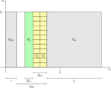
Figure 8: Sketch of the geometry in the proof of Proposition 6.6. The sets are so defined that $\Omega$ is covered by their union, this is ensured by making $\Omega_{\textrm{B}}$ have width $l_{1}$.

Proof of Proposition 6.6.

We cover $\Omega=(0,l_{1})\times(0,l_{2})$ by the union of three sets: a boundary layer region $\Omega_{\textrm{BL}}$, a branching region $\Omega_{\textrm{BR}}$, and a bulk region $\Omega_{\textrm{B}}$,

$$\Omega\subset\tilde{\Omega}:=\Omega_{\textrm{BL}}\cup\Omega_{\textrm{BR}}\cup\Omega_{\textrm{B}}$$

where

$$\Omega_{\textrm{BL}}:=(0,\varepsilon)\times(0,l_{2}),\quad\Omega_{\textrm{BR}}:=[\varepsilon,\varepsilon+l_{\textrm{BR}}]\times(0,l_{2}),\quad\Omega_{\textrm{B}}:=(\varepsilon+l_{\textrm{BR}},\varepsilon+l_{\textrm{BR}}+l_{1})\times(0,l_{2}),$$

and where the boundary layer width $\varepsilon$ and the branching region width $l_{\textrm{BR}}$ are to be determined. In particular, $l_{\textrm{BR}}$ will be chosen by summing up the optimal widths of the individual branching steps. We construct the test function on $\tilde{\Omega}$ and then restrict to $\Omega$, which only decreases the energy; note that $\Omega\subset\tilde{\Omega}$ for any choice of the parameters. In the boundary layer region $\Omega_{\textrm{BL}}$ we use the construction $(\tilde{u},\tilde{v},\tilde{w})$ from Section 5.2 with $h=h_{N}$ and $\delta=\delta_{N}$ to be determined. In the bulk region $\Omega_{\textrm{B}}$ we use the construction from Section 5.1 with $l=l_{1}$, $h=h_{0}$ and $\delta=\delta_{0}$, again to be determined. We assume $h_{N}=2^{N}h_{0}$ for some $N\in\mathbb{N}$, also to be determined. (We assume without loss of generality as in Section 5.3 that $2h_{0}$ divides $l_{2}$ and use the construction from Section 5.1 on the $l_{2}/2h_{0}$ rectangles $(\varepsilon+l_{\textrm{BR}},\varepsilon+l_{\textrm{BR}}+l_{1})\times(2h_{0}(j-1),2h_{0}j)$, $j\in\{1,\ldots,l_{2}/2h_{0}\}$.)

We split up the branching region $\Omega_{\textrm{BR}}$ into $N$ vertical strips $\Omega_{i}$ of width $2L_{i}$, $i\in\{0,\ldots,N-1\}$:

$$\Omega_{\textrm{BR}}=\bigcup_{i=0}^{N-1}\Omega_{i},\qquad\Omega_{i}:=\Bigg{\{}[0,2L_{i}]+\varepsilon+\sum_{k=i+1}^{N-1}2L_{k}\Bigg{\}}\times(0,l_{2}).$$

Note that the strips are labelled from left to right in decreasing order $\Omega_{N-1},\ldots,\Omega_{1},\Omega_{0}$. The total width of the branching region is defined by $l_{\textrm{BR}}:=\sum_{i=0}^{N-1}2L_{i}$, while the values of the $L_{i}$’s are chosen below. Let $h_{i+1}=h_{i}/2$, $i\in\{0,\ldots,N-1\}$. Then each strip is split into $l_{2}/2h_{i}$ rectangles $R_{i}^{j}$ of height $2h_{i}$, see Figure 8.

$$\Omega_{i}=\bigcup_{j=1}^{l_{2}/2h_{i}}R_{i}^{j},\qquad R_{i}^{j}:=\Bigg{\{}[0,2L_{i}]+\varepsilon+\sum_{k=i+1}^{N-1}2L_{k}\Bigg{\}}\times\Bigg{\{}[0,2h_{i}]+(j-1)2h_{i}\Bigg{\}}.$$

Finally, we split each rectangle $R_{i}^{j}$ into two rectangles $U_{i}^{j}$, $V_{i}^{j}$ of width $L_{i}$:

$$R_{i}^{j}=U_{i}^{j}\cup V_{i}^{j}$$

$$U_{i}^{j} :=\Bigg{\{}[0,L_{i}]+\varepsilon+\sum_{k=i+1}^{N-1}2L_{k}\Bigg{\}}\times\Bigg{\{}[0,2h_{i}]+(j-1)2h_{i}\Bigg{\}},$$

$$V_{i}^{j} :=\Bigg{\{}[L_{i},2L_{i}]+\varepsilon+\sum_{k=i+1}^{N-1}2L_{k}\Bigg{\}}\times\Bigg{\{}[0,2h_{i}]+(j-1)2h_{i}\Bigg{\}}.$$

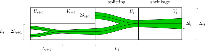
Figure 9: Sketch of the geometry in the proof of Proposition 6.6. The area marked green is the set where $w>0$.

Let $\delta_{0}>\delta_{1}>\cdots>\delta_{N}$. On the rectangles $U_{i}^{j}$ we use the fold splitting construction from Lemma 6.3 with $h=h_{i}$, $\delta=\delta_{i+1}$, $l=L_{i}$. This is admissible provided that

(6.28) $$\delta_{i+1}\leq h_{i+1}=\frac{h_{i}}{2}\text{ and }h_{i}\leq L_{i}\,.$$

On the rectangles $V_{i}^{j}$ we use the fold shrinkage construction from Lemma 6.4 with $h=h_{i}$, $\delta=\delta_{i}$, $\lambda=\delta_{i+1}/\delta_{i}$, $l=L_{i}$, see Figure 9. This is admissible provided that

(6.29) $$\delta_{i}\leq h_{i}\leq L_{i}\text{ and }\frac{1}{4}\delta_{i}\leq\delta_{i+1}\leq\delta_{i}\,.$$

By Lemmas 6.1, 6.3 and 6.4 the energy of the displacement satisfies

(6.30) $$I^{(\sigma,\gamma)}[\mathboit u,w,U_{i}^{j}\cup V_{i}^{j}]\leq c\gamma\delta_{i}L_{i}+c(\sigma l_{1})^{2}\frac{L_{i}h_{i}}{\delta_{i}^{2}}+c\frac{h_{i}^{6}}{\delta_{i}L_{i}^{3}}.$$

Equating terms on the right-hand leads to the optimality conditions

$$\delta_{i}\sim(\sigma l_{1})^{2/3}\gamma^{-1/3}h_{i}^{1/3},\quad L_{i}\sim(\sigma l_{1})^{-1/2}\delta_{i}^{1/4}h_{i}^{5/4}.$$

In order to enforce (6.28) and (6.29) we choose

$$\delta_{i}:=\min\left\{h_{i},(\sigma l_{1})^{2/3}\gamma^{-1/3}h_{i}^{1/3}\right\},\quad L_{i}:=\max\left\{h_{i},(\sigma l_{1})^{-1/2}\delta_{i}^{1/4}h_{i}^{5/4}\right\},\quad i\in\{0,\ldots,N-1\}.$$

We only have to verify the second condition in (6.29). Obviously $\delta_{i+1}\leq\delta_{i}$. At the same time, $h_{i+1}=h_{i}/2$ implies $\delta_{i+1}\geq\delta_{i}/2$.

To complete the proof we need to consider two cases: $\gamma\geq 1$, $\gamma<1$.

Case $\gamma\geq 1$: First we choose $h_{N}$ and $\delta_{N}$, the size of the folding pattern in the boundary layer, by equating terms in equation (5.6). This gives

(6.31) $$\varepsilon:=h_{N}:=\sigma l_{1}\gamma,\quad\delta_{N}:=\sigma l_{1}$$

and

(6.32) $$I^{(\sigma,\gamma)}[\mathboit u,w,\Omega_{\textrm{BL}}]\leq Cl_{2}\varepsilon=Cl_{1}l_{2}\sigma\gamma.$$

Observe that $\delta_{N}\leq\varepsilon$ since $\gamma\geq 1$ and so the bound (5.6) is valid (in particular, $h\leq l_{2}$ since $\sigma\gamma\leq 1$). Now we determine which of the two values is taken by $\delta_{i}$, $i\in\{0,\ldots,N-1\}$. Note that

$$h_{i}\geq(\sigma l_{1})^{2/3}\gamma^{-1/3}h_{i}^{1/3}\quad\Longleftrightarrow\quad h_{i}\geq\sigma l_{1}\gamma^{-1/2}.$$

But for all $i$

$$h_{i}\geq h_{N}=\sigma l_{1}\gamma\geq\sigma l_{1}\gamma^{-1/2}$$

since $\gamma\geq 1$. Therefore for all $i\in\{0,\ldots,N-1\}$

(6.33) $$\delta_{i}=(\sigma l_{1})^{2/3}\gamma^{-1/3}h_{i}^{1/3}$$

and, inserting in the definition of $L_{i}$,

$$L_{i}=\max\left\{h_{i},(\sigma l_{1})^{-1/3}\gamma^{-1/12}h_{i}^{4/3}\right\}.$$

Note that

$$h_{i}\leq(\sigma l_{1})^{-1/3}\gamma^{-1/12}h_{i}^{4/3}\quad\Longleftrightarrow\quad h_{i}\geq\sigma l_{1}\gamma^{1/4}.$$

But for all $i$

$$h_{i}\geq h_{N}=\sigma l_{1}\gamma\geq\sigma l_{1}\gamma^{1/4}$$

since $\gamma\geq 1$. Therefore

(6.34) $$L_{i}=(\sigma l_{1})^{-1/3}\gamma^{-1/12}h_{i}^{4/3}\quad\textrm{for all }i\in\{0,\ldots,N-1\}.$$

It remains to choose $h_{0}$ (equivalently $N$). We do this by balancing the energy in the bulk region $\Omega_{\textrm{B}}$ with the energy in the branching region $\Omega_{\textrm{BR}}$. The same computation as in Lemma 5.1 shows that the energy in $\Omega_{\textrm{B}}$ satisfies

(6.35) $$I^{(\sigma,\gamma)}[\mathboit u,w,\Omega_{\textrm{B}}]\leq C\frac{l_{2}}{2h_{0}}\left((\sigma l_{1})^{2}\frac{l_{1}h_{0}}{\delta_{0}^{2}}+2{\gamma}l_{1}\delta_{0}\right)=Cl_{1}l_{2}(\sigma l_{1})^{2/3}\gamma^{2/3}h_{0}^{-2/3}.$$

Inserting (6.33) and (6.34) in (6.30) leads to

$$I^{(\sigma,\gamma)}[\mathboit u,w,U_{i}^{j}\cup V_{i}^{j}]\leq C(\sigma l_{1})^{1/3}\gamma^{7/12}h_{i}^{5/3}.$$

Therefore the energy in $\Omega_{\textrm{BR}}$ satisfies

$$I^{(\sigma,\gamma)}[\mathboit u,w,\Omega_{\textrm{BR}}] \leq C\sum_{i=0}^{N-1}\frac{l_{2}}{2h_{i}}(\sigma l_{1})^{1/3}\gamma^{7/12}h_{i}^{5/3}=C\sum_{i=0}^{N-1}l_{2}(\sigma l_{1})^{1/3}\gamma^{7/12}h_{i}^{2/3}$$

(6.36) $$=C\sum_{i=0}^{N-1}l_{2}(\sigma l_{1})^{1/3}\gamma^{7/12}(2^{-i}h_{0})^{2/3}\leq Cl_{2}(\sigma l_{1})^{1/3}\gamma^{7/12}h_{0}^{2/3}.$$

Equating the energy bounds for $\Omega_{\textrm{B}}$ and $\Omega_{\textrm{BR}}$ gives

$$l_{1}l_{2}(\sigma l_{1})^{2/3}\gamma^{2/3}h_{0}^{-2/3}=l_{2}(\sigma l_{1})^{1/3}\gamma^{7/12}h_{0}^{2/3}\quad\Longleftrightarrow\quad h_{0}=l_{1}\sigma^{1/4}\gamma^{1/16}.$$

(Here we have assumed that the equation $l_{1}\sigma\gamma=h_{N}=2^{-N}h_{0}=2^{-N}l_{1}\sigma^{1/4}\gamma^{1/16}$ has an integer solution $N$. In general this will not be the case. We obtain the same energy bound, however, by defining $h_{0}=l_{1}\sigma^{1/4}\gamma^{1/16}$, $\tilde{N}=\lfloor|\log_{2}(l_{1}\sigma\gamma/h_{0})|\rfloor$, $h_{i}=2^{-i}h_{0}$, $i\in\{1,\ldots,\tilde{N}\}$.) We remark that $h_{0}\geq h_{N}$ because $\gamma\leq\sigma^{-4/5}$. Substituting $h_{0}=l_{1}\sigma^{1/4}\gamma^{1/16}$ into (6.35) and (6.36) yields

$$I^{(\sigma,\gamma)}[\mathboit u,w,\Omega_{\textrm{B}}\cup\Omega_{\textrm{BR}}]\leq Cl_{1}l_{2}\sigma^{1/2}\gamma^{5/8}.$$

By combing this and (6.32) we find that

$$I^{(\sigma,\gamma)}[\mathboit u,w,\Omega]\leq Cl_{1}l_{2}(\sigma^{1/2}\gamma^{5/8}+\sigma\gamma).$$

But since $\sigma\gamma\leq 1$ and $\gamma\geq 1$

$$\sigma\gamma=\sigma^{1/2}\gamma^{5/8}(\sigma\gamma)^{1/2}\gamma^{-1/8}\leq\sigma^{1/2}\gamma^{5/8}$$

and we obtain the desired result.

Case $\gamma<1$: In this case we choose $\varepsilon$, $h_{N}$ and $\delta_{N}$ as for the case $\gamma=0$ (see [7]):

(6.37) $$\varepsilon=h_{N}=\delta_{N}=l_{1}\sigma.$$

(Compare (6.37) to (6.31).) Substituting these into equation (5.6) gives

(6.38) $$I^{(\sigma,\gamma)}[\mathboit u,w,\Omega_{\textrm{BL}}]\leq Cl_{1}l_{2}\sigma(1+\gamma)\leq Cl_{1}l_{2}\sigma$$

since $\gamma<1$. Now we determine $\delta_{i}$ for $i\in\{0,\ldots,N-1\}$. In this case

$$h_{N}=\sigma l_{1}<\sigma l_{1}\gamma^{-1/2}.$$

Let $I$ be the largest value of $i<N$ such that $h_{i}\geq\sigma l_{1}\gamma^{-1/2}$ (if there is none, $I=-1$). We have

(6.39) $$\delta_{i}=(\sigma l_{1})^{2/3}\gamma^{-1/3}h_{i}^{1/3}\;\textrm{ for }i\in\{0,\ldots,I\},\qquad\delta_{i}=h_{i}\;\textrm{ for }i\in\{I+1,\ldots,N-1\}.$$

Therefore

$$L_{i}=\left\{\begin{array}[]{ll}\max\left\{h_{i},(\sigma l_{1})^{-1/3}\gamma^{-1/12}h_{i}^{4/3}\right\}&\textrm{if }i\in\{0,\ldots,I\},\\ \max\left\{h_{i},(\sigma l_{1})^{-1/2}h_{i}^{3/2}\right\}&\textrm{if }i\in\{I+1,\ldots,N-1\}.\end{array}\right.$$

Since $\gamma<1$ and $h_{i}\geq h_{N}=\sigma l_{1}$, it is easy to check that

(6.40) $$L_{i}=\left\{\begin{array}[]{ll}(\sigma l_{1})^{-1/3}\gamma^{-1/12}h_{i}^{4/3}&\textrm{if }i\in\{0,\ldots,I\},\\ (\sigma l_{1})^{-1/2}h_{i}^{3/2}&\textrm{if }i\in\{I+1,\ldots,N-1\}.\end{array}\right.$$

It remains to choose $h_{0}$. We do this as for the case $\gamma\geq 1$ by balancing the energy in the bulk region $\Omega_{\textrm{B}}$ with the energy in the branching region $\Omega_{\textrm{BR}}$. From (6.35) we see that the energy in the bulk region satisfies

(6.41) $$I^{(\sigma,\gamma)}[\mathboit u,w,\Omega_{\textrm{B}}]\leq\begin{cases}Cl_{1}l_{2}(\sigma l_{1})^{2/3}\gamma^{2/3}h_{0}^{-2/3}&\text{ if }h_{0}\geq\sigma l_{1}\gamma^{-1/2},\\ Cl_{1}l_{2}(\sigma l_{1})^{2}h_{0}^{-2}&\text{ if }h_{0}<\sigma l_{1}\gamma^{-1/2}.\end{cases}$$

Inserting equations (6.39), (6.40) in (6.30),

$$I^{(\sigma,\gamma)}[\mathboit u,w,U_{i}^{j}\cup V_{i}^{j}]\leq C\left\{\begin{array}[]{ll}(\sigma l_{1})^{1/3}\gamma^{7/12}h_{i}^{5/3}&\textrm{if }i\in\{0,\ldots,I\},\\ (\sigma l_{1})^{-1/2}\gamma h_{i}^{5/2}+(\sigma l_{1})^{3/2}h_{i}^{1/2}&\textrm{if }i\in\{I+1,\ldots,N-1\}.\end{array}\right.$$

Therefore the energy in $\Omega_{\textrm{BR}}$ satisfies

$$I^{(\sigma,\gamma)}[\mathboit u,w,\Omega_{\textrm{BR}}] \leq C\sum_{i=0}^{I}\frac{l_{2}}{2h_{i}}(\sigma l_{1})^{1/3}\gamma^{7/12}h_{i}^{5/3}+C\sum_{i=I+1}^{N-1}\frac{l_{2}}{2h_{i}}\left((\sigma l_{1})^{-1/2}\gamma h_{i}^{5/2}+(\sigma l_{1})^{3/2}h_{i}^{1/2}\right)$$

$$\leq Cl_{2}\left((\sigma l_{1})^{1/3}\gamma^{7/12}h_{0}^{2/3}+(\sigma l_{1})^{-1/2}\gamma h_{I+1}^{3/2}+(\sigma l_{1})^{3/2}h_{N-1}^{-1/2}\right)$$

$$\leq Cl_{2}\left((\sigma l_{1})^{1/3}\gamma^{7/12}h_{0}^{2/3}+\sigma l_{1}\gamma^{1/4}+\sigma l_{1}\right)$$

since $h_{I-1}<\sigma l_{1}\gamma^{-1/2}$ and $h_{N-1}=2h_{N}=2\sigma l_{1}$. Since $\gamma<1$,

(6.42) $$I^{(\sigma,\gamma)}[\mathboit u,w,\Omega_{\textrm{BR}}]\leq Cl_{2}\left((\sigma l_{1})^{1/3}\gamma^{7/12}h_{0}^{2/3}+\sigma l_{1}\right).$$

It remains to choose $h_{0}$. If $\gamma<\sigma$, we expect the second term on the right-hand side of (6.42) will dominate the energy, therefore it suffices to choose $h_{0}$ so that the others are not bigger. Focusing on the second row of (6.41) one easily sees that $h_{0}=\sigma^{1/2}l_{1}$ is the appropriate choice (this is the same choice used in [7, 8]). In particular, since $\gamma<\sigma$ this obeys $h_{0}<\sigma l_{1}\gamma^{-1/2}$, hence is consistent. Adding together (6.41), (6.38) and (6.42) yields in this case

$$I^{(\sigma,\gamma)}[\mathboit u,w,\Omega]\leq Cl_{1}l_{2}(\sigma+\sigma^{2/3}\gamma^{7/12})\leq 2Cl_{1}l_{2}\sigma.$$

If instead $\gamma\geq\sigma$, we choose $h_{0}$ by equating the $h_{0}$ term on the right-hand side of (6.42) with the first row in the right-hand side of (6.41). This gives

$$h_{0}=l_{1}\sigma^{1/4}\gamma^{1/16}$$

as in the case $\gamma\geq 1$. This is consistent since $h_{0}\geq\sigma l_{1}\gamma^{-1/2}$ is the same as $\gamma\geq\sigma^{4/3}$, which is true in this case. Then adding together (6.41), (6.38) and (6.42) yields

$$I^{(\sigma,\gamma)}[\mathboit u,w,\Omega]\leq Cl_{1}l_{2}(\sigma+\sigma^{1/2}\gamma^{5/8})$$

as required. ∎

Appendix A Derivation of the Model and Rescaling

In this appendix we derive the energy (1.1). We model the two-layer material (an elastic film on a substrate) described in the introduction with an energy consisting of two parts, an elastic energy for the thin film and a bonding energy for the interaction between the film and the substrate. We take the elastic energy to be the von Kármán energy, which penalises extension (stretching and compression) and bending:

(A.1) $$\hat{I}_{\mathrm{vK}} :=\frac{Eh_{\mathrm{f}}}{2(1-\nu^{2})}\int_{\Omega}\left\{(1-\nu)\left|\frac{D\mathboit u+(D\mathboit u)^{\textrm{T}}}{2}+\frac{Dw\otimes Dw}{2}-\varepsilon_{*}\mathrm{Id}\right|^{2}\right.$$

$$\left.\phantom{\frac{Eh_{\mathrm{f}}}{2(1-\nu^{2})}\int_{\Omega}}\quad+\nu\left|\mathrm{tr}\left(\frac{D\mathboit u+(D\mathboit u)^{\textrm{T}}}{2}+\frac{Dw\otimes Dw}{2}-\varepsilon_{*}\mathrm{Id}\right)\right|^{2}\right\}\,d\mathboit x$$

$$\phantom{==}+\frac{Eh_{\mathrm{f}}^{3}}{24(1-\nu^{2})}\int_{\Omega}\left\{(1-\nu)|D^{2}w|^{2}+\nu(\Delta w)^{2}\right\}\,d\mathboit x$$

where $\Omega=(0,l_{1})\times(0,l_{2})$ is the set of material points $(x,y)$ of the film, $h_{\textrm{f}}$ is the thickness of the film, $E$ is the Young’s Modulus, and $\nu$ is the Poisson ratio. The functions $\mathboit u(x,y)=(u(x,y),v(x,y))$ and $w(x,y)$ are the in-plane and transversal (vertical) displacements of the film from the isotropically compressed state $((1-\varepsilon_{*})x,(1-\varepsilon_{*})y,0)$, where $0<\varepsilon_{*}<1$ is the compression ratio. Note that ${\varepsilon}_{*}=0$ corresponds to no compression and ${\varepsilon}_{*}=1$ corresponds to total compression. Thus $(u,v,w)=(0,0,0)$ corresponds to the isotropically compressed state of the film and $(u,v,w)=(\varepsilon_{*}x,\varepsilon_{*}y,0)$ corresponds to the relaxed, natural state. The substrate is taken to be at height $z=0$. Therefore the transversal displacement $w$ must satisfy the constraint $w\geq 0$ (since the film cannot go below the substrate). If $w(x,y)=0$ then the material point $(x,y)$ of the film is bonded down to the substrate.

For the energy scaling analysis that we perform we can set the Poisson ratio $\nu$ equal to zero without loss of generality since the terms of (A.1) with factor $\nu$ can be bound from above and below by those without, as shown in [7, Appendix B].

The interfacial force between the thin film and the substrate is an attractive van der Waals force. We model it in a simple way with a bonding energy $\hat{I}_{\textrm{Bo}}$ that penalises debonding from the substrate:

(A.2) $$\hat{I}_{\textrm{Bo}}:=\gamma^{*}|\{(x,y)\in\Omega\,:\,w(x,y)>0\}|$$

where $\gamma^{*}$ is a constant depending on the material properties of the film and the substrate. In more sophisticated models $I_{\textrm{Bo}}$ would also depend on the size of $w$, i.e., how far the film is from the substrate.

Thus the total energy we assign to the system is

(A.3) $$\hat{I}:=\hat{I}_{\textrm{vK}}+\hat{I}_{\textrm{Bo}}.$$

On the boundary $\{x=0\}$ we assume that the film is fixed to the substrate and satisfies the clamped boundary conditions

(A.4) $$u(0,y)=0,\quad v(0,y)=0,\quad w(0,y)=0,\quad Dw(0,y)=0.$$

(Note that in the experiments of [27] the film is actually fixed to a buffer layer and satisfies slightly different boundary conditions. This is discussed in Appendix B.) The film is free on the rest of its boundary, $\{x=l_{1}\}\cup\{y=0\}\cup\{y=l_{2}\}$.

Rescaling.

In order to reduce the number of parameters we define rescaled variables, denoted with a superscript $*$, by

(A.5) $$\mathboit u=:2\varepsilon_{*}\mathboit u^{*},\qquad w=:(2\varepsilon_{*})^{1/2}\,w^{*}.$$

By substituting from equation (A.5) into equation (A.3), multiplying by $2(1-\nu^{2})/(Eh_{\mathrm{f}}\varepsilon_{*}^{2})$, setting $\nu=0$, and dropping all the superscripts * for convenience, we obtain a new energy $I^{(\sigma,{\gamma})}$:

(A.6) $$I^{(\sigma,{\gamma})}[\mathboit u,w,l_{1},l_{2}] =\int_{x=0}^{l_{1}}\!\int_{y=0}^{l_{2}}|D\mathboit u+(D\mathboit u)^{\mathrm{T}}+Dw\otimes Dw-\mathrm{Id}|^{2}\,dx\,dy$$

$$\phantom{=}+(\sigma l_{1})^{2}\int_{x=0}^{l_{1}}\!\int_{y=0}^{l_{2}}|D^{2}w|^{2}\,dx\,dy+{\gamma}|\{(x,y)\in\Omega\,:\,w(x,y)>0\}|$$

where $\sigma$ is the rescaled film thickness and ${\gamma}$ is the rescaled bonding energy per unit area:

(A.7) $$\sigma:=\frac{h_{\mathrm{f}}}{l_{1}(6\varepsilon_{*})^{1/2}},\qquad{\gamma}:=\frac{2(1-\nu^{2}){\gamma}^{*}}{Eh_{\mathrm{f}}\varepsilon_{*}^{2}}=\frac{2{\gamma}^{*}}{Eh_{\mathrm{f}}\varepsilon_{*}^{2}}\quad(\textrm{since }\nu=0).$$

Throughout this paper we refer to ${\gamma}$ as the bonding strength, although note that it also depends on the unscaled film thickness $h_{\textrm{f}}$. Equation (A.6) is exactly equation (1.1) given in the Introduction.

Appendix B Upper Bounds for Buffer Layers with Nonzero Thickness

In the experiments of [27] the film is not clamped to the substrate, but rather to a thin buffer layer, and satisfies clamped boundary conditions of the form

(B.1) $$u(0,y)=0,\quad v(0,y)=0,\quad w(0,y)=h_{\mathrm{b}},\quad Dw(0,y)=\mathbf{0}$$

where $h_{\mathrm{b}}>0$ is the thickness of the buffer layer. In this paper we considered the unphysical case $h_{\mathrm{b}}=0$ in order to simplify the analysis. In this appendix we show that the upper bounds of Theorem 2.1 also hold when $h_{\mathrm{b}}$ is sufficiently small. Recall that $\Omega=(0,l_{1})\times(0,l_{2})$. Define

$$V_{h_{\textrm{b}}}=\left\{(\mathboit u,w)\in H^{1}(\Omega;\mathbb{R}^{2})\times H^{2}(\Omega):w=h_{\textrm{b}},\,\mathboit u=Dw=\mathbf{0},\,\textrm{ on }\{0\}\times(0,l_{2}),\;w\geq 0\right\}.$$

Theorem B.1 (Upper Bounds for $h_{\textrm{b}}>0$).

Let $0<l_{1}\leq l_{2}$, $\sigma\in(0,1)$, ${\gamma}\geq 0$. Assume that $h_{\textrm{b}}$ satisfies

$$0\leq\frac{h_{\textrm{b}}}{l_{1}}\leq\min\{\sigma,\sigma^{-1}{\gamma}^{-3/2}\}.$$

Then there exists admissible displacement fields $(\mathboit u,w)\in V_{h_{\textrm{b}}}$ satisfying the same upper bounds as in Theorem 2.1.

Proof.

We construct displacement fields satisfying the required upper bounds by simply appending to the constructions used to prove Theorem 2.1 a boundary layer in which the film is bent upwards from height $0$ to height $h_{\textrm{b}}$. Let $\eta>0$ be the boundary layer thickness. For $x\in[0,\eta]$, $y\in[0,l_{2}]$ define

(B.2) $$u=\frac{1}{2}x,\quad v=0,\quad w=h_{\textrm{b}}\left[1-\psi\left(\frac{x}{\eta}\right)\right]$$

where $\psi\in C^{2}(\mathbb{R})$ is a function with $\psi(t)=0$ for $t\leq 0$, $\psi(t)=1$ for $t\geq 1$. For $x\geq\eta$, define $u$, $v$, $w$ as in the proof of Theorem 2.1 (except that $u$ is replaced with $u+\eta/2$). The energy $E_{\textrm{BL}}^{\eta}$ of $(u,v,w)$ in the boundary layer $(0,\eta)\times(0,l_{2})$ satisfies

(B.3) $$E_{\textrm{BL}}^{\eta}\leq l_{2}\eta\left(\frac{h_{\textrm{b}}^{4}}{\eta^{4}}+(\sigma l_{1})^{2}\frac{h_{\textrm{b}}^{2}}{\eta^{4}}+1+\gamma\right)\leq l_{2}\eta\left(2(\sigma l_{1})^{2}\frac{h_{\textrm{b}}^{2}}{\eta^{4}}+1+\gamma\right)$$

since we assumed that $h_{\textrm{b}}\leq\sigma l_{1}$. We choose

(B.4) $$\eta=(\sigma l_{1}h_{\textrm{b}})^{1/2}\max\{1,\gamma\}^{-1/4}$$

so that

(B.5) $$E_{\textrm{BL}}^{\eta}\leq l_{2}(\sigma l_{1}h_{\textrm{b}})^{1/2}\max\{1,\gamma\}^{3/4}.$$

For each regime it is easy to check that this boundary layer energy is no greater than the energy of the constructions given in Theorem 2.1. ∎

This is the simplest possible modification of the proof of Theorem 2.1 and we do not claim that the bound $h_{\textrm{b}}/l_{1}<\min\{\sigma,\sigma^{-1}{\gamma}^{-3/2}\}$ is sharp.

Appendix C Poincaré Constant

In this section we prove the Poincaré inequality (3.2). It is sufficient to prove the following:

Lemma C.1.

Let $Q=(0,1)\times(0,1)$ be the unit square and $\mathboit f\in C^{2}(Q;\mathbb{R}^{2})$. Let $\mathboit f$ be zero on at least half of the square:

$$|\{\mathboit x\in Q:\mathboit f(\mathboit x)=\mathbf{0}\}|\geq\frac{1}{2}.$$

Then

$$\int_{Q}|\mathboit f|^{2}\,d\mathboit x\leq\int_{Q}|D\mathboit f|^{2}\,d\mathboit x.$$

Proof.

First we recall the Poincaré inequality in one dimension. Let $\mathboit g:[0,1]\to\mathbb{R}^{2}$. Write $\mathboit g$ as the Fourier cosine series (the Fourier series of the even extension of $g$ to $[-1,1]$)

$$\mathboit g(x)=\frac{\hat{\mathboit g}_{0}}{2}+\sum_{k=1}^{\infty}\hat{\mathboit g}_{k}\cos(\pi kx),\qquad\hat{\mathboit g}_{k}=2\int_{0}^{1}\mathboit g(x)\cos(\pi kx)\,dx.$$

Let $\overline{\mathboit g}=\hat{\mathboit g}_{0}/2=\int_{0}^{1}\mathboit g(x)\,dx$. By Parseval’s Theorem

(C.1) $$\int_{0}^{1}|\mathboit g(x)-\overline{\mathboit g}|^{2}\,dx=\frac{1}{2}\sum_{k=1}^{\infty}|\hat{\mathboit g}_{k}|^{2}=\frac{1}{2\pi^{2}}\sum_{k=1}^{\infty}\frac{1}{k^{2}}|\pi k\hat{\mathboit g}_{k}|^{2}\leq\frac{1}{2\pi^{2}}\sum_{k=1}^{\infty}|\pi k\hat{\mathboit g}_{k}|^{2}=\frac{1}{\pi^{2}}\int_{0}^{1}|\mathboit g^{\prime}(x)|^{2}\,dx,$$

which is the Poincaré inequality in one dimension. Let

$$\mathboit a(x)=\int_{0}^{1}\mathboit f(x,y)\,dy,\qquad\overline{\mathboit a}=\int_{0}^{1}\mathboit a(x)\,dx=\int_{Q}\mathboit f(x,y)\,dxdy.$$

By equation (C.1)

$$\int_{0}^{1}|\mathboit a(x)-\overline{\mathboit a}|^{2}\,dx\leq\frac{1}{\pi^{2}}\int_{0}^{1}|\mathboit a^{\prime}(x)|^{2}\,dx\leq\frac{1}{\pi^{2}}\int_{0}^{1}\int_{0}^{1}|\mathboit f_{x}|^{2}\,dxdy,$$

$$\int_{0}^{1}|\mathboit f(x,y)-\mathboit a(x)|^{2}\,dy\leq\frac{1}{\pi^{2}}\int_{0}^{1}|\mathboit f_{y}|^{2}\,dy.$$

Therefore

(C.2) $$\int_{Q}|\mathboit f-\overline{\mathboit a}|^{2}\,dxdy\leq 2\left(\int_{Q}|\mathboit f-\mathboit a|^{2}\,dxdy+\int_{Q}|\mathboit a-\overline{\mathboit a}|^{2}\,dxdy\right)\leq\frac{2}{\pi^{2}}\int_{Q}|D\mathboit f|^{2}\,dxdy.$$

Let $U=\{\mathboit x\in Q:\mathboit f(\mathboit x)=\mathbf{0}\}$. We have

(C.3) $$\frac{1}{2}|\overline{\mathboit a}|^{2}\leq|U||\overline{\mathboit a}|^{2}=\int_{U}|\mathboit f-\overline{\mathboit a}|^{2}\,dx\leq\frac{2}{\pi^{2}}\int_{Q}|D\mathboit f|^{2}\,dxdy.$$

Observe that

$$\int_{Q}|\mathboit f-\overline{\mathboit a}|^{2}\,d\mathboit x=\int_{Q}|\mathboit f|^{2}\,d\mathboit x-|\overline{\mathboit a}|^{2}.$$

By combining this with estimates (C.2) and (C.3) we complete the proof:

$$\int_{Q}|\mathboit f|^{2}\,d\mathboit x=\int_{Q}|\mathboit f-\overline{\mathboit a}|^{2}\,d\mathboit x+|\overline{\mathboit a}|^{2}\leq\frac{6}{\pi^{2}}\int_{Q}|D\mathboit f|^{2}\,d\mathboit x.$$

∎

Acknowledgements.

The authors would like to thank O. G. Schmidt and other members of the Institute for Integrative Nanosciences, IFW Dresden (including P. Cendula, S. Kiravittaya and Y. F. Mei) for interesting discussions about the experiments that were the motivation for this paper. This work was partially supported by the Deutsche Forschungsgemeinschaft through the Sonderforschungsbereich 1060 “The mathematics of emergent effects”.

References

- [1] R. K. Annabattula, J. M. Veenstra, Y. F. Mei, O. G. Schmidt, and P. R. Onck, Self-organization of linear nanochannel networks, Phys. Rev. B 81 (2010), 224114.
- [2] B. Audoly, Stability of straight delamination blisters, Phys. Rev. Lett. 83 (1999), 4124–4127.
- [3] B. Audoly and A. Boudaoud, Self-similar structures near boundaries in strained systems, Phys. Rev. Lett. 91 (2003), 086105.
- [4] B. Audoly, B. Roman, and A. Pocheau, Secondary buckling patterns of a thin plate under in-plane compression, Eur. Phys. J. B 27 (2002), 7–10.
- [5] J. Bedrossian and R. V. Kohn, Blister patterns and energy minimization in compressed thin films on compliant substrates, Comm. Pure Appl. Math. 68 (2015), 472–510.
- [6] P. Bella and R. V. Kohn, Wrinkles as the result of compressive stresses in an annular thin film, Comm. Pure Appl. Math. 67 (2014), 693–747.
- [7] H. Ben Belgacem, S. Conti, A. DeSimone, and S. Müller, Rigorous bounds for the Föppl-von Kármán theory of isotropically compressed plates, J. Nonlinear Sci. 10 (2000), 661–683.
- [8] , Energy scaling of compressed elastic films, Arch. Rat. Mech. Anal. 164 (2002), 1–37.
- [9] K. Bhattacharya, I. Fonseca, and G. Francfort, An asymptotic study of the debonding of thin films, Arch. Ration. Mech. Anal. 161 (2002), 205–229.
- [10] D. Bourne, S. Conti, and S. Müller, Folding patterns in partially delaminated thin films, Preprint arXiv 1512.06320, to appear in “Innovative numerical approaches for coupled multi-scale problems”, A. Pandolfi and K. Weinberg (eds.), Springer (2015).
- [11] P. Cendula, S. Kiravittaya, Y. F. Mei, Ch. Deneke, and O. G. Schmidt, Bending and wrinkling as competing relaxation pathways for strained free-hanging films, Phys. Rev. B 79 (2009), 085429.
- [12] A. Chambolle, S. Conti, and G. Francfort, Korn-Poincaré inequalities for functions with a small jump set, Preprint hal-01091710v1 (2014).
- [13] R. Choksi, S. Conti, R. V. Kohn, and F. Otto, Ground state energy scaling laws during the onset and destruction of the intermediate state in a type-I superconductor, Comm. Pure Appl. Math. 61 (2008), 595–626.
- [14] R. Choksi, R.V. Kohn, and F. Otto, Energy minimization and flux domain structure in the intermediate state of a type-I superconductor, J. Nonlinear Sci. 14 (2004), 119–171.
- [15] S. Conti, A. DeSimone, and S. Müller, Self-similar folding patterns and energy scaling in compressed elastic sheets, Comp. Meth. Appl. Mech. Eng. 194 (2005), 2534–2549.
- [16] S. Conti and F. Maggi, Confining thin elastic sheets and folding paper, Arch. Rat. Mech. Anal. 187 (2008), 1–48.
- [17] S. Conti and B. Zwicknagl, Low volume-fraction microstructures in martensites and crystal plasticity, preprint arXiv:1507.04521 (2015).
- [18] G. Gioia and M. Ortiz, Delamination of compressed thin films, Adv. Appl. Mech. 33 (1997), 119–192.
- [19] , Determination of thin-film debonding parameters from telephone-cord measurements, Acta Mater. 46 (1998), 169–175.
- [20] R. Huang and S. H. Im, Dynamics of wrinkle growth and coarsening in stressed thin films, Phys. Rev. Lett. 74 (2006), 026214.
- [21] L. Ionov, Biomimetic 3D self-assembling biomicroconstructs by spontaneous deformation of thin polymer films, J. Mater. Chem. 22 (2012), 19366–19375.
- [22] W. Jin and R.V. Kohn, Singular perturbation and the energy of folds, J. Nonlinear Sci. 10 (2000), 355–390.
- [23] W. Jin and P. Sternberg, Energy estimates of the von Kármán model of thin-film blistering, J. Math. Phys. 42 (2001), 192–199.
- [24] R. V. Kohn and S. Müller, Branching of twins near an austenite-twinned-martensite interface, Phil. Mag. A 66 (1992), 697–715.
- [25] , Surface energy and microstructure in coherent phase transitions, Comm. Pure Appl. Math. 47 (1994), 405–435.
- [26] R.V. Kohn and H.-M. Nguyen, Analysis of a compressed thin film bonded to a compliant substrate: the energy scaling law, J. Nonlinear Sci. 23 (2013), 343–362.
- [27] Y. Mei, D. J. Thurmer, F. Cavallo, S. Kiravittaya, and O. G. Schmidt, Semiconductor sub-micro-/nanochannel networks by deterministic layer wrinkling, Advanced Materials 19 (2007), 2124–2128.
- [28] M. Ortiz and G. Gioia, The morphology and folding patterns of buckling-driven thin-film blisters, J. Mech. Phys. Solids 42 (1994), 531–559.
- [29] Y. Pomeau, Buckling of thin plates in the weakly and strongly nonlinear regimes, Phil. Mag. B 78 (1998), 235–242.
- [30] H. Vandeparre, M. Piñeirua, F. Brau, B. Roman, J. Bico, C. Gay, W. Bao, C. N. Lau, P. M. Reis, and P. Damman, Wrinkling hierarchy in constrained thin sheets from suspended graphene to curtains, Phys. Rev. Lett. 106 (2001), 224301.
- [31] B. Zwicknagl, Microstructures in low-hysteresis shape memory alloys: Scaling regimes and optimal needle shapes, Arch. Ration. Mech. Anal. 213 (2014), 355–421.