Photoacoustic Tomography With Spatially Varying Compressibility and Density

Abstract

This paper investigates photoacoustic tomography with two spatially varying acoustic parameters, the compressibility and the density. We consider the reconstruction of the absorption density parameter (imaging parameter of Photoacoustics) with complete and partial measurement data. We investigate and analyze three different numerical methods for solving the imaging problem and compare the results.

Keywords: Photoacoustic imaging, spatially varying compressibility and density, variable sound speed, regularization, time reversal.

1 Introduction

Photoacoustic Imaging (PAI) is a novel technique for tomographical imaging of small biological or medical specimens. The method makes use of the fact that an object expands after being exposed to ultrashort electromagnetic radiation, and emits an ultrasonic wave (see e.g. [32, 28]). The resulting acoustic pressure is assumed to be proportional to the electromagnetic absorption, which is the imaging parameter of Photoacoustics. It provides detailed anatomical and functional information.

Opposed to the conventional photoacoustic imaging [32, 28], which is based on the assumption that the compressibility and density of the medium are constant (and thus in turn the sound speed), this paper assumes both of these parameters spatially varying. The mathematical model describing the propagation of the ultrasonic pressure considered here is

$$\kappa(x)y^{\prime\prime}(x,t)-\nabla\cdot\left(\rho(x)^{-1}\nabla y(x,t)\right) =0\text{ in }\mathbbm{R}^{n}\times(0,\infty)$$ (1)

$$y(x,0) =f(x)\text{ in }\mathbbm{R}^{n}$$

$$y^{\prime}(x,0) =0\text{ in }\mathbbm{R}^{n}.$$

Here, $\kappa$ is the material compressibility, $\rho$ denotes the density and $f$ denotes the amount of absorbed energy, i.e. the imaging parameter that encodes the material properties of physiological interest in PAI. We emphasize that the speed of sound is given by $c(x)=\frac{1}{\sqrt{\kappa\rho}}$ and that this equation is more general than

$$y^{\prime\prime}(x,t)-c^{2}(x)\Delta y(x,t) =0\text{ in }\mathbbm{R}^{n}\times(0,\infty)$$ (2)

$$y(x,0) =f(x)\text{ in }\mathbbm{R}^{n}$$

$$y^{\prime}(x,0) =0\text{ in }\mathbbm{R}^{n},$$

which also describes acoustic wave propagation in the case of variable sound speed. The latter equation is derived from Equation 1 under the additional assumption that $\rho$ is spatially slowly varying. For further details on the derivation of Equation 1 from fluid- and thermodynamics, we refer to [7, Chapter 8.1].

The photoacoustic reconstruction consists in determining the function $f$ from measurement data of $y$ on a surface $S\subseteq\partial\Omega$ over time $(0,T)$.

There exists a huge amount of literature on reconstruction formulas in the case $c\equiv 1$, see for instance [34, 30, 29, 33, 31, 17, 16] to name but a few. Time reversal in the case of variable sound speed has been studied for instance in [2, 14, 21, 19, 26, 15]. Time reversal for photoacoustic imaging based on Equation 1 as well as on Equation 2 has been given in [21] - note that both associated wave operators are special cases of the general operator from [21]. Their theory has been generalized to the elastic wave equation in [24].

In this paper we focus on numerical realization and regularization theory of photoacoustic imaging based on Equation 1 with different numerical methods. Most closely related to our numerical approach is a time reversal algorithm from [25], which employs the formula Equation 27 below. Recently we applied iterative regularization techniques in the case of variable sound speed [6] and compared it with time reversal. The goal here is to generalize time reversal and iterative regularization for photoacoustic imaging in the case of spatially variable density and compressibility. A convergence in the least-squares-sense is thereby guaranteed by standard results from regularization theory (see e.g. [10, 8]).

The paper is organized as follows: In section 2 we analyze the mathematical equations describing wave propagation in the case of spatially variable compressibility and density. Imaging based on this model is analyzed in section 3. Numerical results are presented for three different methods; Time reversal, Neumann series, and Landweber iteration in section 4. The latter two seem to be new for the presented equation. We also investigate the case of partial measurement data.

1.1 Notation

In the beginning we summarize the basic notation, which is used throughout the paper.

$\Omega$ denotes a non-empty, open, bounded and connected domain in $\mathbbm{R}^{n}$ with Lipschitz and piecewise $C^{1}$-boundary $\partial\Omega$. Moreover, $S\subseteq\partial\Omega$ is connected and relatively open. The vector $\bm{n}(x)$, with $x\in\partial\Omega$, denotes the outward pointing unit normal vector of $\Omega$. The absorption density $f$, the compressibility $\kappa$ and the density $\rho$ are supposed to satisfy:

• $\kappa,\rho\in C^{1}(\mathbbm{R}^{n})$, satisfying $0<\rho_{\min}\leq\rho(x)\leq\rho_{\max}$, $0<\kappa_{\min}\leq\kappa(x)\leq\kappa_{\max}$. We also define $c_{\max}:=(\kappa_{\min}\rho_{\min})^{-1/2}$. Moreover, we assume that $\kappa,\rho$ are constant in $\mathcal{C}\Omega$ and satisfy $\kappa\rho=1$ there.

• The absorption density function $f$ has support in $\Omega$: $\text{supp}(f)\subseteq\Omega$.

For the sake of simplicity of notation we omit space and time arguments of functions whenever this is convenient and does not lead to confusions.

We use the following Hilbert spaces:

• We denote by $L^{2}(\Omega)=\left\{\phi\in L^{2}(\mathbbm{R}^{n}):\phi\equiv 0\text{ in }\mathcal{C}\Omega\right\}$, where $\mathcal{C}\Omega$ denotes the complement of $\Omega$, with inner product

  $$\left<\phi_{1},\phi_{2}\right>_{L^{2}(\Omega)}=\int_{\mathbbm{R}^{n}}\phi_{1}\phi_{2}dx.$$

• For $\hat{\Omega}=\Omega$ or $\mathbbm{R}^{n}$:

  • Let $H_{0}^{1}(\hat{\Omega})$ be the closure of differentiable functions on $\mathbbm{R}^{n}$ with compact support in $\hat{\Omega}$, associated with the non-standard (but equivalent) inner product

    $$\left<\phi_{1},\phi_{2}\right>_{1;\kappa,\rho}=\int_{\mathbbm{R}^{n}}\kappa\phi_{1}\phi_{2}+\rho^{-1}\nabla\phi_{1}\cdot\nabla\phi_{2}dx.$$ (3)

    The associated norm is denoted by $\left\|\phi\right\|_{1;\kappa,\rho}$.

  • The seminorm associated to the inner product

    $$\left<\phi_{1},\phi_{2}\right>_{1;\rho}=\int_{\mathbb{R}^{n}}\rho^{-1}\nabla\phi_{1}\cdot\nabla\phi_{2}dx$$ (4)

    is denoted by $\lvert\phi\rvert_{1;\rho}$.

  • The norm associated with the inner product

    $$\left<\phi_{1},\phi_{2}\right>_{1}=\int_{\hat{\Omega}}\phi_{1}\phi_{2}+\nabla\phi_{1}\cdot\nabla\phi_{2}dx$$

    is denoted by $\left\|\phi\right\|_{1}$.

  • The norms $\left\|\phi\right\|_{1}$ and $\left\|\phi\right\|_{1;\kappa,\rho}$ are equivalent. In fact, we have

    $$\sqrt{\min\left\{\kappa_{\min},{\rho_{\max}^{-1}}\right\}}\left\|\phi\right\|_{1}\leq\left\|\phi\right\|_{1;\kappa,\rho}\leq\sqrt{\max\left\{\kappa_{\max},{\rho_{\min}^{-1}}\right\}}\left\|\phi\right\|_{1}\,,$$ (5)

    $$\qquad\text{ for all }\phi\in H_{0}^{1}(\hat{\Omega}).$$

• $L^{2}(S)$ denotes the standard Hilbert space of square integrable functions on $\partial\Omega$ with support in $S$, together with the inner product

  $$\left<\phi_{1},\phi_{2}\right>_{L^{2}(S)}=\int_{S}\phi_{1}(x)\phi_{2}(x)dS(x).$$

  $L^{2}(\Sigma)$ denotes the standard Hilbert space of square integrable functions on $\partial\Omega\times(0,T)$ with support in $\Sigma:=S\times(0,T)$, together with the inner product

  $$\left<\phi_{1},\phi_{2}\right>_{L^{2}(\Sigma)}=\int_{0}^{T}\int_{S}\phi_{1}(x,t)\phi_{2}(x,t)dS(x)dt.$$

  The induced norms are denoted by $\left\|\cdot\right\|_{L^{2}(S)}$, $\left\|\cdot\right\|_{L^{2}(\Sigma)}$.

  $C_{0}^{\infty}(\Sigma)$ denotes the space of smooth functions with support in $\Sigma$.

• The trace operator $\gamma_{\Omega}:H^{1}(\mathbbm{R}^{n})\to L^{2}(\partial\Omega)$ restricts functions defined on $\mathbbm{R}^{n}$ onto $\partial\Omega$, respectively. This operator is the composition of the standard trace operator $\gamma:H^{1}(\Omega)\to L^{2}(\partial\Omega)$ and the restriction operator $R:H^{1}(\mathbbm{R}^{n})\to H^{1}(\Omega)$, which are both bounded [1, Theorem 5.22], and thus itself bounded. We denote

  $$\mathcal{C}_{\gamma}:=\left\|\gamma\circ R\right\|.$$ (6)

2 Direct Problem of Wave Propagation

In this section we are analyzing the wave operator $L$ mapping the absorption density $f$ onto the solution $y$ of Equation 1 restricted to $\Sigma$:

$$L:H_{0}^{1}(\Omega)\rightarrow L^{2}(\Sigma),\quad f\mapsto y|_{\Sigma}.$$ (7)

First, we show that the operator $L$ is bounded. Analogous to [6], we define the total wave energy by

$$E(t;y):=\frac{1}{2}\int_{\mathbbm{R}^{n}}\kappa y^{\prime}{}^{2}+\rho^{-1}\left|\nabla y\right|^{2}dx.$$ (8)

The time derivative of $E$, taking into account Equation 1, is

$$E^{\prime}(t;y)=\int_{\mathbbm{R}^{n}}\kappa y^{\prime\prime}y^{\prime}-\nabla\cdot\left(\rho^{-1}\nabla y\right)y^{\prime}dx=0\text{ for all }t>0.$$

Consequently,

$$E(t;y)=E(0;y)=\frac{1}{2}\lvert f\rvert_{1;\rho}^{2}\text{ for all }t>0.$$ (9)

This, together with Equation 8 shows that

$$\int_{\mathbbm{R}^{n}}\kappa y^{\prime}{}^{2}dx\leq\lvert f\rvert_{1;\rho}^{2}\text{ and }\lvert y(t)\rvert_{1;\rho}\leq\lvert f\rvert_{1;\rho}\text{ for all }t>0.$$ (10)

A-priori this inequality does not provide a bound for $y$ in the whole $\mathbbm{R}^{n}$ with respect to the standard $H^{1}$-norm. This is provided for instance by the following lemma:

Lemma 2.1.

Let $y$ be the solution of Equation 1, then

$$\left\|y(t)\right\|_{1;\kappa,\rho}\leq\mathcal{C}(T)\left\|f\right\|_{1;\kappa,\rho},\qquad\text{ for all }t\in(0,T),$$ (11)

where

$$\mathcal{C}(T):=\sqrt{\max\left\{1+2T^{2},2\right\}}.$$

Proof.

For arbitrary $\hat{t}\in(0,T)$ it follows from Equation 10 that:

$$\int_{\mathbbm{R}^{n}}\kappa(x)(y(x,t)-y(x,0))^{2}dx=\int_{\mathbbm{R}^{n}}\kappa(x)\left(\int_{0}^{\hat{t}}y^{\prime}(x,\hat{t})d\hat{t}\right)^{2}dx$$

$$\leq \hat{t}\int_{0}^{t}\int_{\mathbbm{R}^{n}}\kappa y^{\prime}{}^{2}dxd\hat{t}\leq T^{2}\lvert f\rvert_{1;\rho}^{2}.$$

With the elementary inequality $(a-b)^{2}\geq\frac{1}{2}a^{2}-b^{2}$ it follows that

$$\int_{\mathbbm{R}^{n}}\kappa(x)(y(x,t))^{2}dx$$

$$\leq 2\int_{\mathbbm{R}^{n}}\kappa(x)(y(x,t)-y(x,0))^{2}dx+2\int_{\mathbbm{R}^{n}}\kappa(x)(y(x,0))^{2}dx$$

$$\leq 2T^{2}\lvert f\rvert_{1;\rho}^{2}+2\left\|\sqrt{\kappa}f\right\|_{L^{2}(\mathbb{R}^{n})}^{2}.$$

This, together with Equation 10 shows the assertion.

Now, we prove boundedness of $L$:

Theorem .

The operator $L:H_{0}^{1}(\Omega)\to L^{2}(\Sigma)$ is bounded and

$$\left\|L\right\|\leq\frac{\mathcal{C}_{\gamma}\mathcal{C}(T)\sqrt{T}}{\sqrt{\min\left\{\kappa_{\min},{\rho_{\max}^{-1}}\right\}}}.$$ (12)

Proof.

For given $f$ let $y$ be the solution of Equation 1. From Equation 8 it follows that the solution $y$ of Equation 11 is in $H^{1}(\mathbbm{R}^{n})$ for every $t>0$. Thus from Equation 6 and Equation 11 it follows that

$$\left\|y\right\|_{L^{2}(\Sigma)}^{2}=\int_{0}^{T}\int_{\partial\Omega}y^{2}(t)dS(x)dt\leq\mathcal{C}_{\gamma}^{2}\int_{0}^{T}\left\|y(t)\right\|_{1}^{2}dt\leq\frac{\mathcal{C}_{\gamma}^{2}\mathcal{C}(T)^{2}T\left\|f\right\|_{1;\kappa,\rho}^{2}}{\min\left\{\kappa_{\min},{\rho_{\max}^{-1}}\right\}}.$$

Remark :

From [23, Theorem 1] it follows that the trace $L[f]$ is in fact in $H^{3/4}_{\text{loc}}\left(\partial\Omega\times(0,T)\right)$. Therefore, by finite speed of propagation (section 2), if we in addition assume that $f$ is supported away from $\partial\Omega$, $L[f]$ is in fact in $H^{3/4}\left(\partial\Omega\times(0,T)\right)$. The proof does not follow in a straightforward way from standard trace results, but utilizes the theory of Fourier integral operators and microlocal analysis. In special cases, this result can be further improved, see [21, Remark 5] and also [4, 5]. For instance, for $\Omega$ strictly convex, we have $L[f]\in H^{1}\left(\partial\Omega\times(0,T)\right)$. As a consequence, $L:H^{1}_{0}(\Omega)\to L^{2}(\Sigma)$ is compact, because it is a composition of bounded and a compact operator, using the fact that the embedding from $H^{1}(\partial\Omega\times(0,T))$ to $L^{2}(\partial\Omega\times(0,T))$ is compact (see e.g. [3, Theorem 2.34]).

In the following we characterize the adjoint of $L:H_{0}^{1}(\Omega)\to L^{2}(\Sigma)$ on a dense subset of $L^{2}(\Sigma)$. Since $L^{*}:L^{2}(\Sigma)\to H_{0}^{1}(\Omega)$ is bounded (in fact, $\left\|L\right\|=\left\|L^{*}\right\|$), a characterization follows by limits of convergent sequences on dense subsets. Here we characterize $L^{*}$ on $C_{0}^{\infty}(\Sigma)$ first and extend it by convergent sequences to $L^{2}(\Sigma)$.

Definition .

Let $i$ be the embedding operator from $H_{0}^{1}(\Omega)$ to $L^{2}(\Omega)$. Then $i^{*}:L^{2}(\Omega)\to H_{0}^{1}(\Omega)$ is the operator which maps a function $\psi\in L^{2}(\Omega)$ onto the solution of the equation

$$Du=\psi\text{ in }\Omega,\qquad u=0\text{ on }\partial\Omega,$$ (13)

with $D:=\kappa-\nabla\cdot\rho^{-1}\nabla$. In other words $i^{*}=D^{-1}$.

In the following we derive the adjoint $L^{*}$ of the operator $L$, which is required for the implementation of the Landweber iteration below, on a dense subset of $L^{2}(\Sigma)$. The boundedness of $L^{*}$ is guaranteed by elementary Hilbert space theory. Therefore, we get a characterization on $L^{2}(\Sigma)$ by limits of convergent sequences.

Theorem .

For $h\in C_{0}^{\infty}(\Sigma)$ the adjoint of the operator $L$, defined in Equation 7, is given by

$$L^{*}[h]=i^{*}\circ L_{D}^{*}[h]$$ (14)

where

$$L_{D}^{*}[h]=\left.\kappa z^{\prime}(0)\right|_{\Omega},$$ (15)

and $z:=z(h)$ is the weak solution of

$$\kappa z^{\prime\prime}-\nabla\cdot(\rho^{-1}\nabla z) =0\text{ in }\mathbbm{R}^{n}\backslash\partial\Omega\times(0,T),$$ (16)

$$z(T)=z^{\prime}(T) =0\text{ in }\mathbbm{R}^{n},$$

$$\left[z\right]=0,\quad\left[\frac{\partial z}{\partial\bm{n}}\right] =h\text{ on }\Sigma,$$

$$\left[z\right]=0,\quad\left[\frac{\partial z}{\partial\bm{n}}\right] =0\text{ on }\partial\Omega\setminus\Sigma\times(0,T).$$

Here

$$[z]:=z^{+}|_{\Sigma}-z^{-}|_{\Sigma}\text{ and }\left[\frac{\partial z}{\partial\bm{n}}\right]:=\left.\frac{\partial z^{+}}{\partial\bm{n}}\right|_{\Sigma}-\left.\frac{\partial z^{-}}{\partial\bm{n}}\right|_{\Sigma}$$

where $z^{+}:=z|_{\mathcal{C}\Omega\times(0,T)}$ and $z^{-}:=z|_{\Omega\times(0,T)}$.

Proof.

The existence of a weak solution of Equation 16 is analogous to [6, Appendix A], where the transmission problem has been studied for variable sound speed. Multiplying the first equation of Equation 16 by the solution of Equation 1 $y$, it follows that $h\in C^{\infty}_{0}(\Sigma)$:

$$\int_{\Sigma}hL[f]dS(x)dt=\int_{\Sigma}hydS(x)dt=\int_{\Omega}\kappa z^{\prime}(0)fdx$$ (17)

$$= \int_{\Omega}D\left[D^{-1}\left[\kappa z^{\prime}(0)\right]\right]fdx=\left<i^{*}\left[\kappa{z^{\prime}(0)}\right],f\right>_{1;\kappa,\rho}.$$

The following results on finite speed of propagation of the solution of Equation 1 are based on the results from [9].

Definition .

Let ${\tt d}(x):=\operatorname{dist}(x_{0},x)$ be the distance between $x_{0}$ and $x$ with respect to the Riemannian metric $\kappa\rho dx$. Note that this metric is chosen in accordance with the principal symbol of the elliptic operator

$$-\kappa^{-1}\nabla\cdot\left(\rho^{-1}\nabla\,\cdot\,\right)\;.$$

The cone $\mathcal{K}$ with respect to the space-time point $(t_{0},x_{0})$ is defined as

$$\mathcal{K}:=\left\{(x,t):{\tt d}(x)<t_{0}-t\right\}.$$

we further introduce

$$\mathcal{K}_{t}:=\left\{x:{\tt d}(x)<t_{0}-t\right\},$$

the cross-section of $\mathcal{K}$ at fixed time $t$.

Remark :

According to [9, pp. 416] the function ${\tt d}$ solves the PDE

$$\frac{1}{\rho\kappa}|\nabla{\tt d}|^{2}=1,\quad{\tt d}(x_{0})=0.$$ (18)

This relation will be used in the proof of section 2 below.

Theorem .

Let $y$ be the solution of Equation 1. Assume $y^{\prime}\equiv 0$ on $\mathcal{K}_{0}$, then $y\equiv 0$ in $\mathcal{K}$.

Proof.

Let

$$E_{\mathcal{K}_{t}}(t;y):=\frac{1}{2}\int_{\mathcal{K}_{t}}\kappa y^{\prime}{}^{2}+\rho^{-1}\lvert\nabla y\rvert^{2}dx$$ (19)

denote the local energy. Taking the time derivative of $E_{\mathcal{K}_{t}}$, it follows by application of the Leibniz rule for the differentiation of evolving region integrals [9, p.713] that

$$E_{\mathcal{K}_{t}}^{\prime}(t;y)=\int_{\mathcal{K}_{t}}\kappa y^{\prime}y^{\prime\prime}+\rho^{-1}\nabla y\cdot\nabla y^{\prime}dy+\frac{1}{2}\int_{\partial\mathcal{K}_{t}}\left(\kappa y^{\prime}{}^{2}+\rho^{-1}\lvert\nabla y\rvert^{2}\right)\bm{v}\cdot\bm{n}dS(x),$$

where $\bm{v}$ denotes the normal velocity of the moving boundary $\partial C_{t}$ and $\bm{n}$ is the outward pointing unit normal to $\mathcal{K}_{t}$. For a fixed point $x\in\mathcal{K}_{t}$, we have $\bm{v}(x)=\frac{\nabla{\tt d(x)}}{|\nabla{\tt d(x)}|^{2}}$ and $\bm{n}(x)=-\frac{\nabla{\tt d(x)}}{|\nabla{\tt d(x)}|}$. Therefore,

$$E_{\mathcal{K}_{t}}^{\prime}(t;y) =\int_{\mathcal{K}_{t}}\kappa y^{\prime}y^{\prime\prime}+\rho^{-1}\nabla y\cdot\nabla y^{\prime}dy$$ (20)

$$\qquad-\frac{1}{2}\int_{\partial\mathcal{K}_{t}}\left(\kappa y^{\prime}{}^{2}+\rho^{-1}\lvert\nabla y\rvert^{2}\right)\frac{1}{|\nabla{\tt d}|}dS(x)=:A-B\;.$$

By application of Green’s formula, $A$ is rewritten to

$$A=\int_{\mathcal{K}_{t}}y^{\prime}\left(\kappa y^{\prime\prime}-\nabla\cdot\left(\rho^{-1}\nabla y\right)\right)dx+\int_{\partial\mathcal{K}_{t}}\rho^{-1}y^{\prime}\nabla y\cdot\frac{\nabla{\tt d}}{|\nabla{\tt d}|}dS(x).$$

The first term vanishes since $y$ is solution to Equation 1 and thus from Equation 18 it follows that

$$|A|\leq\int_{\partial\mathcal{K}_{t}}\frac{\lvert y^{\prime}\rvert\rho^{-1/2}\lvert\nabla{\tt d}\rvert\lvert\nabla y\rvert\rho^{-1/2}}{\lvert\nabla{\tt d}\rvert}dS(x)=\int_{\partial\mathcal{K}_{t}}\frac{\lvert y^{\prime}\rvert\kappa^{1/2}\lvert\nabla y\rvert\rho^{-1/2}}{\lvert\nabla{\tt d}\rvert}dS(x)\;.$$

Using Cauchy’s inequality, we finally obtain

$$|A|\leq\frac{1}{2}\int_{\partial\mathcal{K}_{t}}\left(\kappa y^{\prime}{}^{2}+\rho^{-1}\lvert\nabla y\rvert^{2}\right)\frac{1}{\lvert\nabla{\tt d}\rvert}dS(x)=B\;.$$

Thus, from Equation 20 it follows that $E_{\mathcal{K}_{t}}^{\prime}(t;y)\leq 0.$

3 Photoacoustic Imaging

The photoacoustic imaging problem can be expressed as the solution of the operator equation:

$$L[f]=m.$$ (21)

Uniqueness of the solution of Equation 21 is closely related to a unique continuation result for the wave equation:

Theorem (Unique Continuation [20, 12, 22]).

Let $u$ be a solution to Equation 1, and $y\equiv 0$ in $(-T,T)\times B_{\varepsilon}(x_{0})$. Then

$$y\equiv 0\text{ in }\left\{(x,t)\in\mathbbm{R}\times\mathbbm{R}^{n}:\operatorname{dist}(x,x_{0})\leq T-|t|\right\}\;.$$

Uniqueness of the solution of Equation 21 requires a sufficiently large observation time

$$T_{0}:=\max\limits_{x\in\mathop{\mathrm{supp}}f}\operatorname{dist}(x,S),$$ (22)

where $\operatorname{dist}(x,S)$ is the distance of $x$ to the closest point $x^{\prime}\in S$ with respect to the Riemannian metric $\kappa\rho dx$.

Corollary (Injectivity of $L$ [21]).

Let $\Omega$ be strictly convex and $T>T_{0}$. Moreover, let $\mathop{\mathrm{supp}}f\subset\Omega$. Then $L[f]=0$ implies $f=0$.

In the following we discuss several numerical algorithms for solving Equation 21.

3.1 Landweber Iteration

We are employing the Landweber’s iteration for solving Equation 21 and compare it with the time reversal methods presented in subsection 3.2, which are the standard references in this field. More efficient iterative regularization algorithms are at hand [11], but these are less intuitive to be compared with time reversal. The Landweber algorithm reads as follows:

$$f_{0}:=0\quad\text{and}\quad f_{k}^{\delta}=f_{k-1}^{\delta}-\omega L^{*}[L[f_{k-1}^{\delta}]-m^{\delta}],\quad k=1,2,\dots,$$ (23)

where $m^{\delta}$ stands for error-prone data with $\left\|m^{\delta}-m\right\|_{L^{2}(\Sigma)}<\delta$, where $m=y|_{\Sigma}$. For a summary of results for Landweber regularization in Photoacoustics we refer to [6] and the references therein.

We emphasize that Landweber’s iteration converges to the minimum norm solution

$$f^{\dagger}=L^{\dagger}[m]\,,$$ (24)

where $L^{\dagger}$ is the Moore-Penrose inverse (see [18] for a survey), if the data $m$ is an element of the range of $L$. This is a property which is relevant when the observation time $T$ is smaller than the critical time $T_{0}$ which guarantees injectivity of $L$.

3.2 Time Reversal

In this subsection, we first state the conventional time reversal and give a remark on necessary assumptions to obtain error estimates for this method. This is followed by a description of a modified time reversal approach, for which a theoretical analysis based on [21] can be provided.

Conventional Time Reversal

We formally define the time reversal operator:

$$\overline{L}[h]=z(\cdot,0),$$ (25)

where $z$ is a solution of

$$\begin{aligned} \kappa z^{\prime\prime}-\nabla\cdot(\rho^{-1}\nabla z)&=0\text{ in }\Omega\times(0,T),\\ z(T)=z^{\prime}(T)&=0\text{ in }\Omega,\\ z&=h\text{ on }\partial\Omega\times(0,T),\\ \end{aligned}$$ (26)

The fundamental difference between $\overline{L}$ and $L^{*}$ is that they are defined via differential equations on $\Omega\times(0,T)$ and $\mathbbm{R}^{n}\times(0,T)$. The conventional time reversal reconstruction [25] consists of computing

$$f_{\text{TR}}=\overline{L}[m]\,.$$ (27)

Remark :

Assume that $S=\partial\Omega$, that $\rho\equiv 1$ and the speed of sound is non-trapping. For this case, Hristova [13, Theorem 2] provides an error estimate for the time reversal method, employing results on the decay of solutions of the wave equation (e.g. [27]).

Neumann Series

Stefanov and Uhlmann [21] define the modified time reversal for Equation 1: Rather than assuming (in most cases unjustified) the initial data $z(T)\equiv 0$ we are again using the harmonic extension of the data term $h(s,T)$, for $s\in\partial\Omega$, as initial datum at $T$. That is, for

$$-\nabla\cdot(\rho^{-1}\nabla\phi)=0\text{ in }\Omega,\text{ with }\phi(\cdot)=m(\cdot,T)\text{ on }\partial\Omega$$

the modified time reversal operator

$$\widetilde{\overline{L}}[h]=z(\cdot,0)$$ (28)

is defined by the solution of equation

$$\begin{aligned} \kappa z^{\prime\prime}-\nabla\cdot(\rho^{-1}z)&=0\text{ in }\Omega\times(0,T),\\ z(T)=\phi,\quad z^{\prime}(T)&=0\text{ in }\Omega,\\ z&=h\text{ on }\partial\Omega\times(0,T).\\ \end{aligned}$$ (29)

Note that this algorithm has not been used as a basis for numerical reconstruction for the generalized Equation 1.

Previously [21] showed stability of the modified time reversal reconstruction under non-trapping conditions and for sufficiently large measurement time for Equation 2. In fact, let $c=(\kappa\rho)^{-1/2}$ be non-trapping [14] and $T_{1}$ denote the time when all singularities have left $\overline{\Omega}$. Then the result is directly convertible to Equation 1:

Theorem (Stability of Modified Time Reversal).

[21, Theorem 1] Let $T>T_{1}$ and $S=\partial\Omega$ be a closed $C^{2}$-surface. Moreover, let the coefficients $\kappa$, $\rho\in C^{\infty}(\mathbbm{R}^{n})$.

Then $\widetilde{\overline{L}}L=Id-K$, where $K$ is a compact operator from $H^{1}_{0}(\Omega)\to H^{1}_{0}(\Omega)$ satisfying $\left\|K\right\|<1$.

Note that [21, Theorem 1] works only for complete boundary measurement data.

By subsection 3.2, the initial value $f$ can be expanded into the Neumann series

$$f=\sum_{j=0}^{\infty}K^{j}[m].$$ (30)

By induction one sees that the $m$-th iterate can be written as

$$f_{k}=f_{k-1}-\widetilde{\overline{L}}[L[f_{k-1}]-m],$$ (31)

where

$$f_{k}=\sum_{j=0}^{k}K^{j}[m].$$

Remark :

Note that with partial data, the Neumann series reconstruction consists in formally applying Equation 30 to the extended data $m_{s}$, where

$$m_{s}=m\text{ in }\Sigma^{\prime}\subset\subset\Sigma\text{ and }m_{s}=0\text{ in }\partial\Omega\setminus\Sigma\times(0,T),$$ (32)

in a way that $m_{s}\in H^{1}(\partial\Omega\times[0,T])$ serves as approximation to $m$ in $\Sigma$.

Let now $S\subset\partial\Omega$ relatively open. To fix the terminology, we define for $(x,\xi)\in\mathbbm{R}^{n}\times\mathbb{S}^{n-1}$ the curve

$$\gamma_{(x,\xi)}(\tau)$$

to be the geodesic (in the Riemannian metric $\kappa\rho dx$) through $x$ in direction $\xi$, where $\tau\in(-\infty,\infty)$ and $\gamma_{(x,\xi)}(0)=x$. Note that

$$\tau_{\pm}(x,\xi)=\max\left\{\tau\geq 0:\gamma_{(x,\xi)}(\pm\tau)\in\overline{\Omega}\right\}.$$

give the (possibly infinite) times when the geodesics leave the domain in positive ($\operatorname{sgn}=+$) resp. negative ($\operatorname{sgn}=-$) direction. Regarding stability [21, Theorem 3] provides the following result, which holds also in the partial data case.

Theorem .

Assume that

$$(\tau_{\text{sgn}}(x,\xi),\gamma_{(x,\xi)}(\tau_{\text{sgn}}(x,\xi))\in\Sigma$$

holds for all $(x,\xi)\in\Omega_{1}\times\mathbb{S}^{n-1}$ in at least one of the two directions $\operatorname{sgn}=+$, $\operatorname{sgn}=-$. Then there exists a constant $C>0$ such that for any $f\in C_{0}^{\infty}(\Omega_{1})$, with $\Omega_{1}\subset\subset\Omega$, the estimate

$$\left\|f\right\|_{H^{1}_{0}(\Omega_{1})}\leq C\left\|Lf\right\|_{H^{1}(\Sigma)}$$

is valid.

4 Numerical Experiments and Results

We compare conventional time reversal Equation 27, the Neumann series approach Equation 31 and the Landweber iteration Equation 23 for the photoacoustic imaging problem based on Equation 1. Similar studies have been performed in [6] for photoacoustic imaging based on Equation 2. Figure 1 displays the involved parameters, including absorption density $f$, material compressibility $\kappa$ and density $\rho$.

For the numerical solution of the involved wave equations Equation 1 and Equation 16, we use a straight-forward adaptation of the BEM-FEM scheme outlined in [6]. Equation 26 and Equation 29 are discretized by finite element discretization.

For the simulation of the data, for all different wave equations, the mesh size has been chosen as $\Delta x=0.0095$ and $\Delta t=\Delta x/(15*c_{\max})$, leading to about $40000$ nodal points in $\Omega$. For all wave equations involved in reconstruction, we use a grid with $\Delta x_{R}=0.01$ and $\Delta t_{R}=\Delta x_{R}/(15*c_{\max})$.

Measurement data are assumed to be recorded on $630$ detection points on the unit circle. In the partial data example, the measurements are restricted to the lower half of the circle.

The total measurement time was varied as multiples of $T_{0}$, which is defined as in Equation 22.

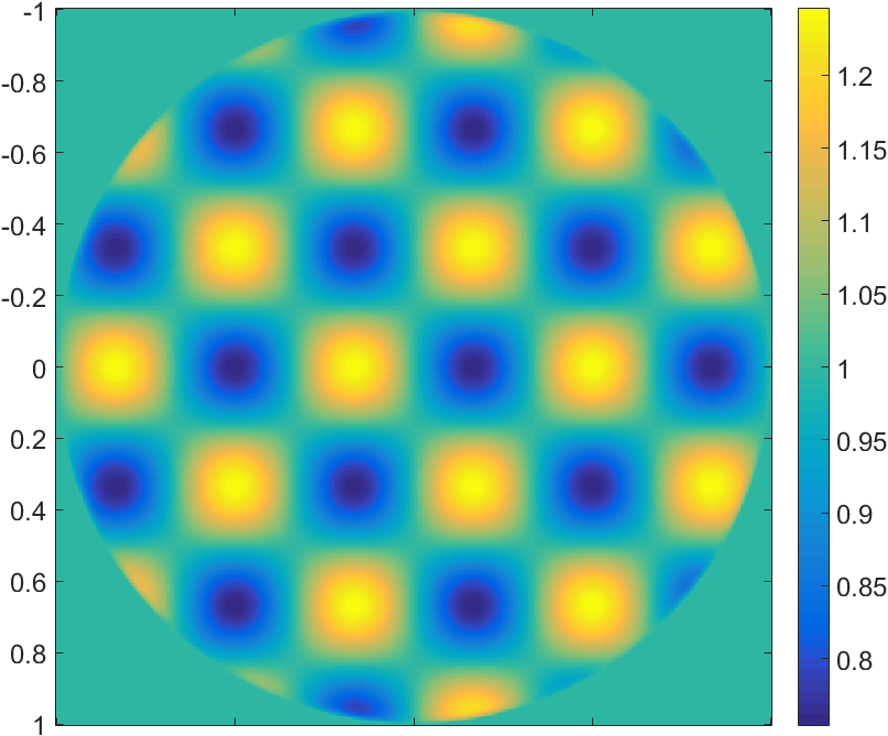
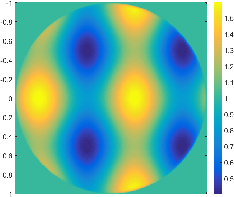
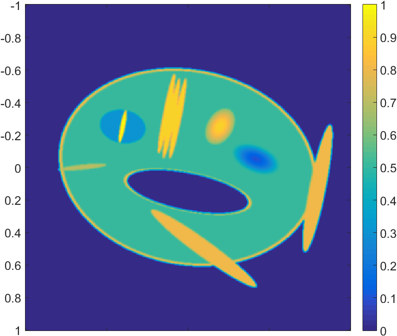
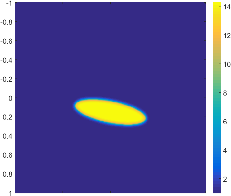
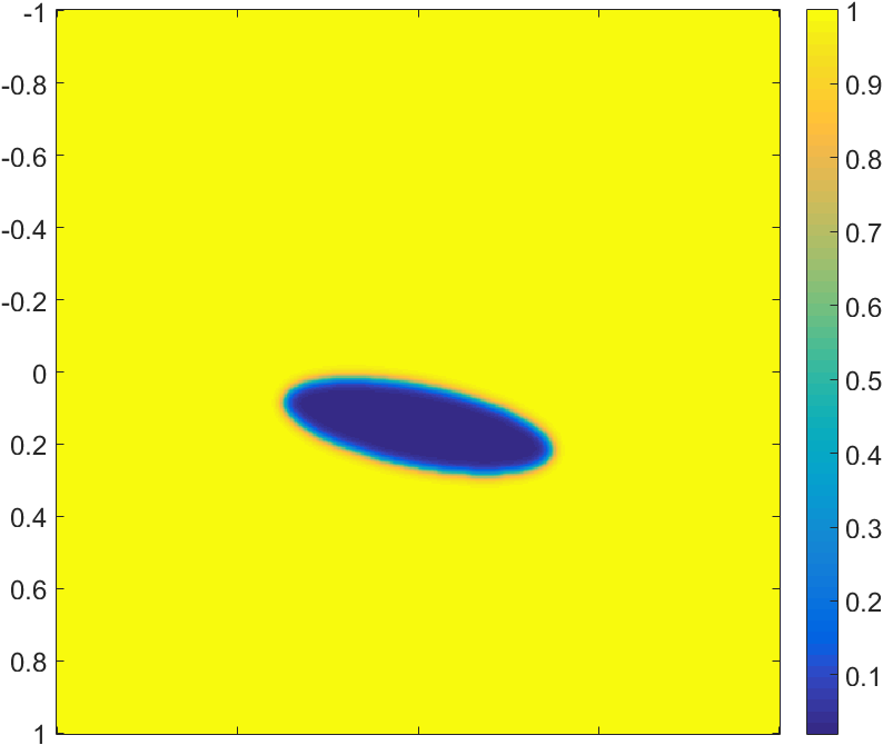
Figure 1: Parameters: First line: Test Example 1 – Mandrill. Second line: Test example 2 – Fish. From left to right: Initial pressure $f$, compressibility $\kappa$, density $\rho$.

4.1 Test Example 1 – Mandrill

We investigate the performance of the different photoacoustic imaging techniques, time reversal, Neumann series and Landweber iteration, respectively, with spatially varying $\kappa$ and $\rho$. We show different test cases

1. for partial measurement data (see Figure 2), where we show the imaging results for $T=2T_{0}$ and $T=4T_{0}$, where $T_{0}$, defined in Equation 22 denotes the minimal time that guarantees unique reconstruction of the absorption density $f$

2. as well as reconstructions from full data in the presence of noise (Figure 3). The noise level is stated as SNR (signal to noise ratio, in dB scale) with respect to the maximum signal value. The examples include moderate noise (SNR $=10$dB) and high noise (SNR $=5$dB).

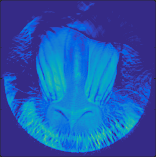
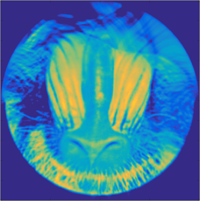
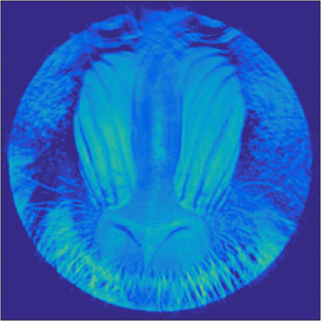
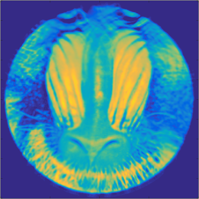
Figure 2: Partial data reconstructions: Data are recorded on the lower unit half-circle and the parameters $\kappa$, $\rho$ are exactly given. Data are noise free and recorded for $T=2T_{0}$, $4T_{0}$. Reconstructions for $T=2T_{0}$, $4T_{0}$ are shown in the first and second line, respectively. From left to right: Time reversal, Neumann series with $k=5$, Landweber iterate $k=5$.

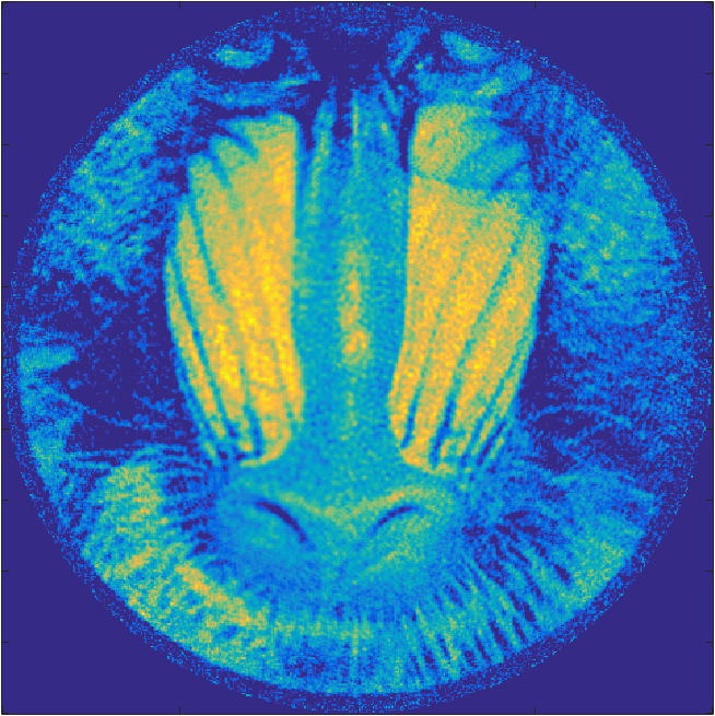
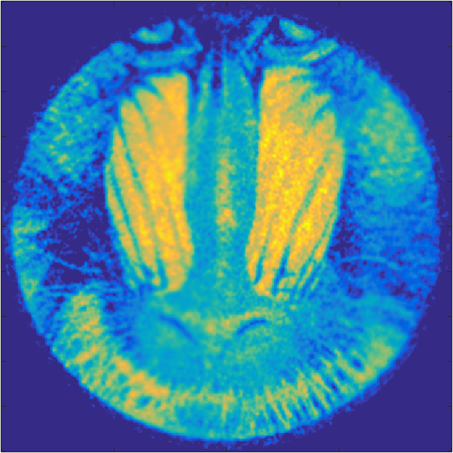
Figure 3: Reconstruction with complete, but noisy measurements and correct parameters $\kappa,\rho$, measurement time $T=2T_{0}$. First line: SNR $=10$dB. Second line: SNR $=5$dB. From left to right: Time reversal, Neumann series with $k=5$, Landweber iterate $k=5$.

4.2 Test Example 2 – Fish

The second test concerns a parameter setting $\kappa,\rho$ and associated sound speed $c=(\kappa\rho)^{-1/2}$, which is reconstructed with inversions (time reversal, Neumann series, Landweber iteration) based on Equation 2.

The phantom simulates a water-like body (e.g. soft tissue) containing an inclusion with significantly different acoustic properties, like the air-filled swim-bladder of a fish (see lower line of Figure 1). We choose the parameters to be bounded in the intervals $0.02\leq\rho\leq 1$ and $1\leq\kappa\leq 14.3$, with high gradients in the transition between the inclusion and the rest of the domain (see also Figure 1).

Moreover, we include the achievable results when only $c=(\kappa\rho)^{-1/2}$ is known, leading to a modeling error in the reconstructions.

1. In the first line of Figure 4 we display the reconstructions with correct parameters $\kappa,\rho$ as depicted in the second line of Figure 1.

1. Next, reconstructions are performed by using the parameters $\kappa_{1}=\kappa\rho$ and $\rho_{1}=1$. This displays the usually considered approximation (see second line of Figure 4).

2. We also try it the other way round by setting $\rho_{2}=\kappa\rho$, and $\kappa_{2}\equiv 1$ (third line of Figure 4). This leads to the wave equation in pure divergence form, and displays the case where the compressibility variations are negligible.

However, in b and c the modeling error leads to severe artifacts near regions of high-gradient regions of the parameters.

4.3 Results

In the presented test examples, all three methods qualitatively reconstruct the same features. Time reversal however fails to give a quantitatively correct results, due to the relatively short measurement times in use. Neumann series and Landweber iteration perform at the same level. As expected from theory, the Landweber reconstructions appear slightly smoother, specifically in Figure 3.

The second test clearly indicates that a modeling error in the reconstruction method can lead to severe artifacts near regions where the parameter gradients are large.

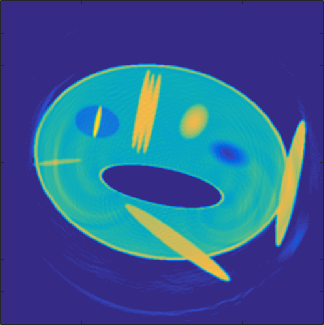
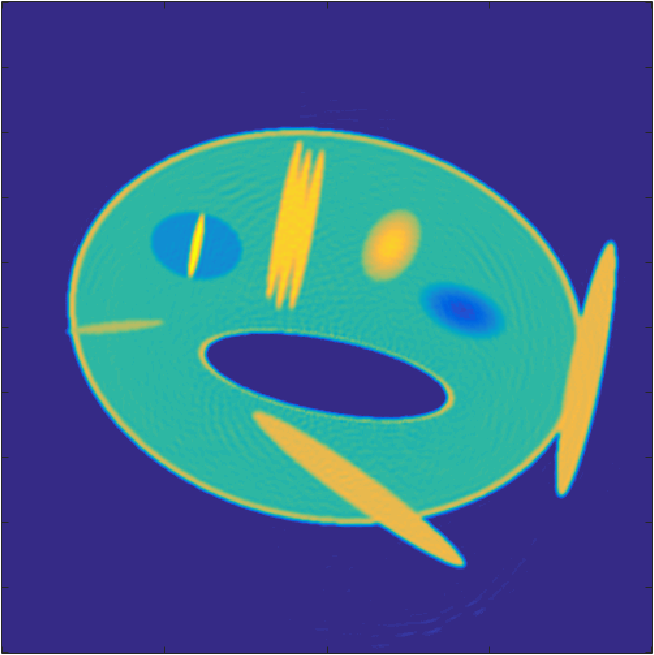
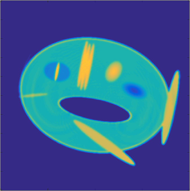
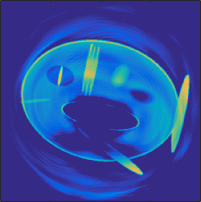
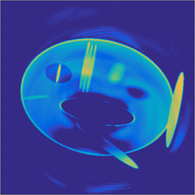
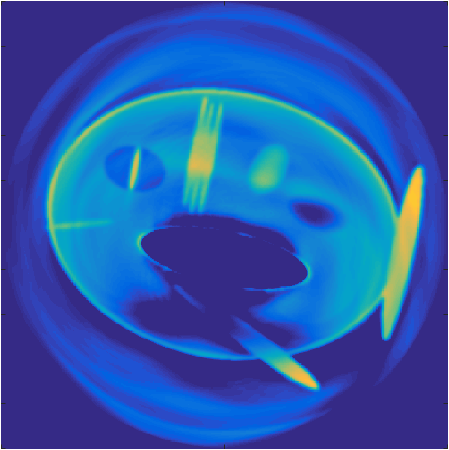
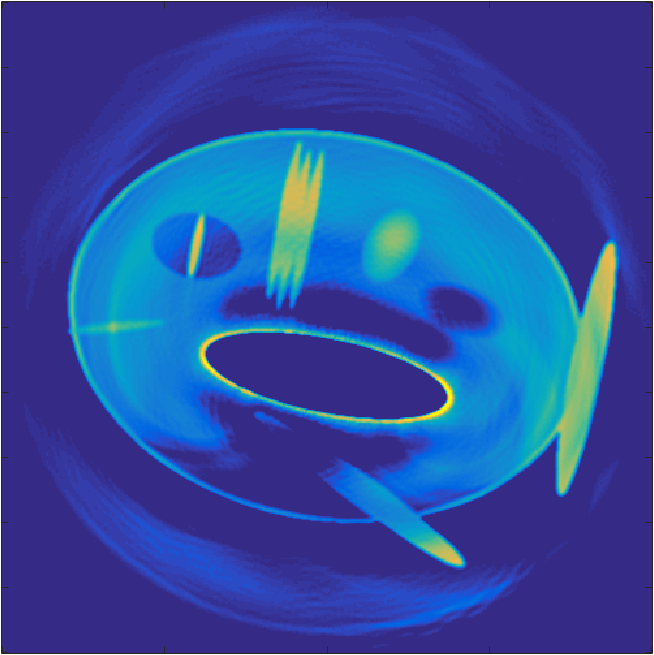
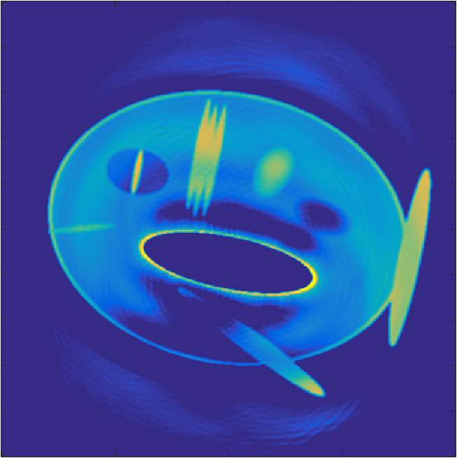
Figure 4: Reconstructions of the Fish phantom with $T=2T_{0}$. First line: Reconstruction using correct parameters $\kappa_{1}=\kappa$, $\rho_{1}=\rho$ as pictured in the second line of Figure 1. Second line: Reconstruction with parameters $\kappa_{1}=\kappa\rho$, $\rho_{1}\equiv 1$. Third line: Reconstruction with parameters $\rho_{1}=\kappa\rho$, $\kappa_{1}\equiv 1$. From left to right: Time reversal, Neumann series with $k=5$, Landweber iterate $k=5$.

5 Conclusions

In this work we have studied photoacoustic imaging based on a general wave model with spatially variable compressibility and density, respectively. We have implemented Neumann series and Landweber iteration for photoacoustic imaging based on this general equation and we compared the result to conventional time reversal as discussed in [25].

The numercial methods for photoacoustic imaging reveal the differences as outlined in Table 1 with respect to convergence, stability and robustness against noise at the present stage of research. Stability is understood in the sense of regularization theory [10], meaning that the Landweber iterates determined by a discrepancy principle approximate the minimum norm solution.

	Time Reversal	Neumann	Landweber
Convergence:			best approx. sol.
measurement time	$T\to\infty$	$T>T_{1}$	$T>0$
sound speed	non-trapping	non-trapping	arbitrary
data	full	full	partial
Stability:			regularized sol.
measurement time	$T>T_{1}$	$T>T_{1}/2$	$T>0$
sound speed	non-trapping	non-trapping	arbitrary
data	full	partial	partial
$L^{2}$-Noise:	no	no	yes

Table 1: Overview on the different photoacoustic imaging methods.

Numerical results show the reconstructions in the case of error prone data and under modeling errors. We emphasize that, so far, an error analysis is only possible for the Landweber iteration.

References

• [1] R. A. Adams. Sobolev Spaces. Academic Press, New York, 1975.
• [2] M. Agranovsky and P. Kuchment. Uniqueness of reconstruction and an inversion procedure for thermoacoustic and photoacoustic tomography with variable sound speed. Inverse Probl., 23(5):2089–2102, 2007.
• [3] T. Aubin. Nonlinear analysis on manifolds, Monge-Ampère equations, volume 252 of Grundlehren der mathematischen Wissenschaften. Springer, New York, 1982.
• [4] G. Bao and W. W. Symes. A trace theorem for solutions of partial differential equations. Math. Methods Appl. Sci., 14(8):553–562, 1991.
• [5] G. Bao and W. W. Symes. Trace regularity for a second order hyperbolic equation with non-smooth coefficients. J. Math. Anal. Appl., 174:370–389, 1993.
• [6] Z. Belhachmi, T. Glatz, and O. Scherzer. A direct method for photoacoustic tomography with inhomogeneous sound speed. Preprint on ArXiv arXiv:1507.01741, University of Vienna, Austria, 2015.
• [7] D. Colton and R. Kress. Inverse acoustic and electromagnetic scattering theory, volume 93 of Applied Mathematical Sciences. Springer-Verlag, Berlin, 1992.
• [8] H. W. Engl, M. Hanke, and A. Neubauer. Regularization of inverse problems. Number 375 in Mathematics and its Applications. Kluwer Academic Publishers Group, Dordrecht, 1996.
• [9] L. C. Evans. Partial Differential Equations, volume 19 of Graduate Studies in Mathematics. American Mathematical Society, Providence, RI, second edition, 2010.
• [10] C. W. Groetsch. The Theory of Tikhonov Regularization for Fredholm Equations of the First Kind. Pitman, Boston, 1984.
• [11] M. Hanke. Conjugate Gradient Type Methods for Ill-Posed Problems, volume 327 of Pitman Research Notes in Mathematics Series. Longman Scientific & Technical, Harlow, 1995.
• [12] L. Hörmander. A uniqueness theorem for second order hyperbolic differential equations. Comm. Partial Differential Equations, 17:699–714, 1992.
• [13] Y. Hristova. Time reversal in thermoacoustic tomography&mdash;an error estimate. Inverse Probl., 25(5):055008 (14pp), 2009.
• [14] Y. Hristova, P. Kuchment, and L. Nguyen. Reconstruction and time reversal in thermoacoustic tomography in acoustically homogeneous and inhomogeneous media. Inverse Probl., 24(5):055006, 2008.
• [15] C. Huang, L. Nie, R. W. Schoonover, L.V. Wang, and M. A. Anastasio. Photoacoustic computed tomography correcting for heterogeneity and attenuation. J. Biomed. Opt., 17:061211, 2012.
• [16] P. Kuchment. The Radon Transform and Medical Imaging. Society for Industrial and Applied Mathematics, Philadelphia, 2014.
• [17] P. Kuchment and L. Kunyansky. Mathematics of thermoacoustic tomography. European J. Appl. Math., 19:191–224, 2008.
• [18] M.Z. Nashed, editor. Generalized inverses and applications. Academic Press [Harcourt Brace Jovanovich Publishers], New York, 1976.
• [19] J. Qia, P. Stefanov, G. Uhlmann, and H. Zhao. An efficient Neumann series-based algorithm for thermoacoustic and photoacoustic tomography with variable sound speed. SIAM J. Imaging Sciences, 4(3):850–883, 2011.
• [20] L. Robbiano. Théorème d’unicité adapté au contrôle des solutions des problèmes hyperboliques. Comm. Partial Differential Equations, 16(4–5):789–800, 1991.
• [21] P. Stefanov and G. Uhlmann. Thermoacoustic tomography with variable sound speed. Inverse Probl., 25(7):075011, 16, 2009.
• [22] D. Tataru. Unique continuation for solutions to pde’s; between Hörmander’s theorem and Holmgren’s theorem. Comm. Partial Differential Equations, 20(5-6):855–884, 1995.
• [23] D. Tataru. On the regularity of boundary traces for the wave equation. Ann. Sc. Norm. Super. Pisa Cl. Sci. (4), 26(1):185–206, 1998.
• [24] J. Tittelfitz. Thermoacoustic tomography in elastic media. Inverse Probl., 28(5):055004, 2012.
• [25] B. E. Treeby and B. T. Cox. K-Wave: MATLAB toolbox for the simulation and reconstruction of photoacoustic wace fields. J. Biomed. Opt., 15:021314, 2010.
• [26] B. E. Treeby, T. K. Varslot, E. Z. Zhang, J. G. Laufer, and P. C. Beard. Automatic sound speed selection in photoacoustic image reconstruction using an autofocus approach. Biomed. Opt. Express, 16(9):090501–3, 2011.
• [27] B. R. Vainberg. On the short wave asymptotic behaviour of solutions of stationary problems and the asymptotic behaviour as $t\to\infty$ of solutions of non-stationary problems. Russ. Math. Surv., 30(2):1–58, 1975.
• [28] L. V. Wang, editor. Photoacoustic Imaging and Spectroscopy. Optical Science and Engineering. CRC Press, Boca Raton, 2009.
• [29] M. Xu and L. V. Wang. Exact frequency-domain reconstruction for thermoacoustic tomography–I: Planar geometry. IEEE Trans. Med. Imag., 21:823–828, 2002.
• [30] M. Xu and L. V. Wang. Time-domain reconstruction for thermoacoustic tomography in a spherical geometry. IEEE Trans. Med. Imag., 21(7):814–822, 2002.
• [31] M. Xu and L. V. Wang. Universal back-projection algorithm for photoacoustic computed tomography. Phys. Rev. E, 71(1), 2005.
• [32] M. Xu and L. V. Wang. Photoacoustic imaging in biomedicine. Rev. Sci. Instruments, 77(4), 2006.
• [33] M. Xu, Y. Xu, and L. V. Wang. Time-domain reconstruction algorithms and numerical simulations for thermoacoustic tomography in various geometries. IEEE Trans. Biomed. Eng., 50(9):1086–1099, 2003.
• [34] Y. Xu, M. Xu, and L. V. Wang. Exact frequency-domain reconstruction for thermoacoustic tomography — II: Cylindrical geometry. IEEE Trans. Med. Imag., 21:829–833, 2002.