Lectures on K-theoretic computations in enumerative geometry

1. Aims & Scope

1.1. K-theoretic enumerative geometry

1.1.1.

These lectures are for graduate students who want to learn how to do the computations from the title. Here I put emphasis on computations because I think it is very important to keep a connection between abstract notions of algebraic geometry, which can be very abstract indeed, and something we can see, feel, or test with code.

While it is a challenge to adequately illustrate a modern algebraic geometry narrative, one can become familiar with main characters of these notes by working out examples, and my hope is that these notes will be placed alongside a pad of paper, a pencil, an eraser, and a symbolic computation interface.

1.1.2.

Modern enumerative geometry is not so much about numbers as it is about deeper properties of the moduli spaces that parametrize the geometric objects being enumerated.

Of course, once a relevant moduli space $\mathbb{M}$ is constructed one can study it as one would study any other algebraic scheme (or stack, depending on the context). Doing this in any generality would appear to be seriously challenging, as even the dimension of some of the simplest moduli spaces considered here (namely, the Hilbert scheme of points of 3-folds) is not known.

1.1.3.

A productive middle ground is to compute the Euler characteristics $\chi(\mathscr{F})$ of naturally defined coherent sheaves $\mathscr{F}$ on $\mathbb{M}$, as representations of a group $G$ of automorphisms of the problem. This goes beyond intersecting natural cycles in $\mathbb{M}$, which is the realm of the traditional enumerative geometry, and is a nutshell description of equivariant K-theoretic enumerative geometry.

The group $G$ will typically be connected and reductive, and the $G$-character of $\chi(\mathscr{F})$ will be a Laurent polynomial on the maximal torus $T\subset G$ provided $\chi(\mathscr{F})$ is a finite-dimensional virtual $G$-module. Otherwise, it will be a rational function on $T$. In either case, it is a very concrete mathematical object, which can be turned and spun to be seen from many different angles.

1.1.4.

Enumerative geometry has received a very significant impetus from modern high energy physics, and this is even more true of its K-theoretic version. From its very origins, K-theory has been inseparable from indices of differential operators and related questions in mathematical quantum mechanics. For a mathematical physicist, the challenge is to study quantum systems with infinitely many degrees of freedom, systems that describe fluctuating objects that have some spatial extent.

While the dynamics of such systems is, obviously, very complex, their vacua, especially supersymmetric vacua, i.e. the quantum states in the kernel of a certain infinite-dimensional Dirac operator

(1)

may often be understood in finite-dimensional terms. In particular, the computations of supertraces

$$\operatorname{str}e^{-\beta\not{D}^{2}}A =\operatorname{tr}_{(\operatorname{Ker}\not{D})_{\textup{even}}}A-\operatorname{tr}_{(\operatorname{Ker}\not{D})_{\textup{odd}}}A$$

(2) $$=\operatorname{str}_{\operatorname{index}\not{D}}A$$

of natural operators $A$ commuting with $\not{D}$ may be equated with the kind of computations that is done in these notes.

Theoretical physicists developed very powerful and insightful ways of thinking about such problems and theoretical physics serves as a very important source of both inspiration and applications for the mathematics pursued here. We will see many examples of this below.

1.1.5.

What was said so far encompasses a whole universe of physical and enumerative contexts. While resting on certain common principles, this universe is much too rich and diverse to be reasonably discussed here.

These lectures are written with a particular goal in mind, which is to introduce a student to computations in two intertwined subjects, namely:

• K-theoretic Donaldson-Thomas theory, and

• quantum K-theory of Nakajima varieties.

Some key features of these theories, and of the relationship between them, may be summarized as follows.

1.2. Quantum K-theory of Nakajima varieties

1.2.1.

Nakajima varieties [Nak1, Nak2] are associated to a quiver (that is, a finite graph with possibly parallel edges and loops), a pair of dimension vectors, and a choice of stability chamber. They form a remarkable family of equivariant symplectic resolutions [Kal2] and have found many geometric and representation-theoretic applications. Their construction will be recalled in Section 4.

For quivers of affine ADE type, and a suitable choice of stability, Nakajima varieties are the moduli spaces of framed coherent sheaves on the corresponding ADE surfaces, e.g. on $\mathbb{C}^{2}$ for a quiver with one vertex and one loop. These moduli spaces play a very important role in supersymmetric gauge theories and algebraic geometry.

For general quivers, Nakajima varieties share many properties of the moduli spaces of sheaves on a symplectic surface. In fact, from their construction, they may be interpreted as moduli spaces of stable objects in certain abelian categories which have the same duality properties as coherent sheaves on a symplectic surface.

1.2.2.

From many different perspectives, rational curves in Nakajima varieties are of particular interest. Geometrically, a map

$$\textup{curve $C$}\to\textup{Moduli of sheaves on a surface $S$}$$

produces a coherent sheaf on a threefold $C\times S$. One thus expects a relation between enumerative geometry of sheaves on threefolds fibered in ADE surfaces and enumerative geometry of maps from a fixed curve to affine ADE Nakajima varieties.

Such a relation indeed exists and has been already profitably used in cohomology [OP1, OP2, MauObl, moop]. For it to work well, it is important that the fibers are symplectic. Also, because the source $C$ of the map is fixed and doesn’t vary in moduli, it can be taken to be a rational curve, or a union of rational curves.

Rational curves in other Nakajima varieties lead to enumerative problems of similar 3-dimensional flavor, even when they are lacking a direct geometric interpretations as counting sheaves on some threefold.

1.2.3.

In cohomology, counts of rational curves in a Nakajima variety $X$ are conveniently packaged in terms of equivariant quantum cohomology, which is a certain deformation of the cup product in ${H}^{\raisebox{1.42262pt}{$\scriptscriptstyle\bullet$}}_{G}(X)$ with deformation base $H^{2}(X)$. A related structure is the equivariant quantum connection, or Dubrovin connection, on the trivial ${H}^{\raisebox{1.42262pt}{$\scriptscriptstyle\bullet$}}_{G}(X)$ bundle with base $H^{2}(X)$.

While such packaging of enumerative information may be performed for an abstract algebraic variety $X$, for Nakajima varieties these structures are described in the language of geometric representation theory, and namely in terms of an action of a certain Yangian $\mathsf{Y}(\mathfrak{g})$ on ${H}^{\raisebox{1.42262pt}{$\scriptscriptstyle\bullet$}}_{G}(X)$. In particular, the quantum connection is identified with the trigonometric Casimir connection for $\mathsf{Y}(\mathfrak{g})$, studied in [TolCas] for finite-dimensional Lie algebras, see also [TV].

The construction of the required Yangian $\mathsf{Y}(\mathfrak{g})$, and the identification of quantum structures in terms of $\mathsf{Y}(\mathfrak{g})$, are the main results of [59]. That work was inspired by conjectures put forward by Nekrasov and Shatashvili [NS1, NS2], on the one hand, and by Bezrukavnikov and his collaborators (see e.g. [Et]), on the other.

A similar geometric representation theory description of quantum cohomology is expected for all equivariant symplectic resolutions, and perhaps a little bit beyond, see for example [FFFR]. Further, there are conjectural links, due to Bezrukavnikov and his collaborators, between quantum connections for symplectic resolutions $X$ and representation theory of their quantizations (see, for example, [BezF, BK, BM, 11, Kal1]), their derived autoequivalences etc.

1.2.4.

The extension [60] of our work [59] with D. Maulik to K-theory requires several new ideas, as certain arguments that are used again and again in [59] are simply not available in K-theory. For instance, in equivariant cohomology, a proper integral of correct dimension is a nonequivariant constant, which may be computed using an arbitrary specialization of the equivariant parameters (it is typically very convenient to set the weight $\hbar$ of the symplectic form to $0$ and send all other equivariant variables to infinity).

By contrast, in equivariant $K$-theory, the only automatic conclusion about a proper pushforward to a point is that it is a Laurent polynomial in the equivariant variables, and, most of the time, this cannot be improved. If this Laurent polynomial does not involve some equivariant variable variable $a$ then this is called rigidity, and is typically shown by a careful study of the $a^{\pm 1}\to\infty$ limit. We will see many variations on this theme below.

Also, very seldom there is rigidity with respect to the weight $\hbar$ of the symplectic form and nothing can be learned from making that weight trivial. Any argument that involves such step in cohomology needs to be modified, most notably the proof of the commutation of quantum connection with the difference Knizhnik-Zamolodchikov connection, see Sections 1.4 and 9 of [59]. In the logic of [59], quantum connection is characterized by this commutation property, so it is very important to lift the argument to K-theory.

One of the goals of these notes is to serve as an introduction to the additional techniques required for working in K-theory. In particular, the quantum Knizhnik-Zamolodchikov connection appears in Section 10.4 as the computation of the shift operator corresponding to a minuscule cocharacter. Previously in Section 8.2 we construct a difference connection which shifts equivariant variables by cocharacters of the maximal torus and show it commutes with the K-theoretic upgrade of the quantum connection. That upgrade is a difference connection that shifts the Kähler variables

$$z\in H^{2}(X,\mathbb{C})\big{/}2\pi iH^{2}(X,\mathbb{Z})$$

by cocharacters of this torus, that is, by a lattice isomorphic to $\operatorname{Pic}(X)$. This quantum difference connection is constructed in Section 8.1.

1.2.5.

Technical differences notwithstanding, the eventual description of quantum $K$-theory of Nakajima varieties is exactly what one might have guessed recognizing a general pattern in geometric representation theory. The Yangian $\mathsf{Y}(\mathfrak{g})$, which is a Hopf algebra deformation of $\mathscr{U}(\mathfrak{g}\otimes\mathbb{C}[t])$, is a first member of a hierarchy in which the Lie algebra

$$\mathfrak{g}\otimes\mathbb{C}[t]=\textup{Maps}(\mathbb{C},\mathfrak{g})$$

is replaced, in turn, by a central extension of maps from

• the multiplicative group $\mathbb{C}^{\times}$, or

• an elliptic curve.

Geometric realizations of the corresponding quantum groups are constructed in equivariant cohomology, equivariant K-theory, and equivariant elliptic cohomology, respectively, see [60, 75] and also [1] for the construction of an elliptic quantum group from Nakajima varieties.

Here we are on the middle level of the hierarchy, where the quantum group is denoted $\mathscr{U}_{\hbar}(\hat{\mathfrak{g}})$. The variable $q$ is the deformation parameter; its geometric meaning is the equivariant weight of the symplectic form. For quivers of finite type, these are identical to Drinfeld-Jimbo quantum groups from textbooks. For other quivers, $\mathscr{U}_{\hbar}(\hat{\mathfrak{g}})$ is constructed in the style of Faddeev, Reshetikhin, and Takhtajan from geometrically constructed $R$-matrices, see [59]. In turn, the construction of $R$-matrices, that is, solutions of the Yang-Baxter equations with a spectral parameter, rests on the $K$-theoretic version of stable envelopes of [60]. We discuss those in Section 9.1.

Stable envelopes in K-theory differ from their cohomological ancestors in one important feature: they depend on an additional parameter, called slope, which is a choice of an alcove of a certain periodic hyperplane arrangement in $\operatorname{Pic}(X)\otimes_{\mathbb{Z}}\mathbb{R}$. This is the same data as appears, for instance, in the study of quantization of $X$ over a field of large positive characteristic. A technical advantage of such slope dependence is a factorization of $R$-matrices into infinite product of certain root $R$-matrices, which generalizes the classical results obtained by Khoroshkin and Tolstoy in the case when the Lie algebra $\mathfrak{g}$ is of finite dimension.

1.2.6.

The identification of the quantum difference connection in term of $\mathscr{U}_{\hbar}(\hat{\mathfrak{g}})$ was long expected to be the lattice part of the quantum dynamical Weyl group action on $K_{G}(X)$. For finite-dimensional Lie algebras, this object was studied by Etingof and Varchenko in [EV] and many related papers, and it was shown in [Bal] to correctly degenerate to the Casimir connection in the suitable limit.

Intertwining operators between Verma modules, which is the main technical tool of [EV], are only available for real simple roots and so don’t yield a large enough dynamical Weyl group as soon as the quiver is not of finite type. However, using root $R$-matrices, one can define and study the quantum dynamical Weyl group for arbitrary quivers. This is done in [75]. Once available, a representation-theoretic identification of the quantum difference connections gives an essentially full control over the theory.

In these notes we stop where the analysis of [75] starts: we show that quantum connection commutes with qKZ, which is one of the key features of dynamical Weyl groups.

1.2.7.

The monodromy of the quantum difference connection is characterized in [1] in terms of an elliptic analog of $\mathscr{U}_{\hbar}(\hat{\mathfrak{g}})$. The categorical meaning of the corresponding operators is an area of active current research.

1.2.8.

These notes are meant to be a partial sample of basic techniques and results, and this is not an attempt to write an A to Z technical manual on the subject, nor to present a panorama of geometric applications that these techniques have.

For instance, one of the most exciting topics in quantum K-theory of symplectic resolutions is the duality, known under many different names including “symplectic duality” or “3-dimensional mirror symmetry”, see [65] for an introduction. Nakajima varieties may be interpreted as the moduli space of Higgs vacua in certain supersymmetric gauge theories, and the computations in their quantum K-theory may be interpreted as indices of the corresponding gauge theories on real 3-folds of the form $C\times S^{1}$. A physical duality equates these indices for certain pairs of theories, exchanging the Kähler parameters on one side with the equivariant parameters on the other.

In the context of these notes, this means that an exchange of the Kähler and equivariant difference equations of Section 8, which may be studied as such and generalizes various dualities known in representation theory. This is just one example of a very interesting phenomenon that lies outside of the scope of these lectures.

1.3. K-theoretic Donaldson-Thomas theory

1.3.1.

Donaldson-Thomas theory, or DT theory for short, is an enumerative theory of sheaves on a fixed smooth quasiprojective threefold $Y$, which need not be Calabi-Yau to point out one frequent misconception. There are many categories similar to the category of coherent sheaves on a smooth threefold, and one can profitably study DT-style questions in that larger context. In fact, we already met with such generalizations in the form of quantum K-theory of general Nakajima quiver varieties. Still, I consider sheaves on threefolds to be the core object of study in DT theories.

An example of a sheaf to have in mind could be the structure sheaf $\mathscr{O}_{C}$ of a curve, or more precisely, a $1$-dimensional subscheme, $C\subset Y$. The corresponding DT moduli space $\mathbb{M}$ is the Hilbert scheme of curves in $Y$ and what we want to compute from them is the K-theoretic version of counting curves in $Y$ of given degree and arithmetic genus satisfying some further geometric constraints like incidence to a given point or tangency to a given divisor.

There exist other enumerative theories of curves, notably the Gromov-Witten theory, and, in cohomology, there is a rather nontrivial equivalence between the DT and GW counts, first conjectured in [mnop1, mnop2] and explored in many papers since. At present, it is not known whether the GW/DT correspondence may be lifted to K-theory, as one stumbles early on trying to mimic the DT computations on the GW side , see for example the discussion in Section 6.1.8.

1.3.2.

Instead, in K-theory there is a different set of challenging conjectures [67] which may serve as one of the goalposts for the development of the theory.

This time the conjectures relate DT counts of curves in $Y$ to a very different kind of curve counts in a Calabi-Yau 5-fold $Z$ which is a total space

(3) $$Z=\begin{matrix}\mathscr{L}_{4}\oplus\mathscr{L}_{5}\\ \downarrow\\ Y\end{matrix}\,,\quad\mathscr{L}_{4}\otimes\mathscr{L}_{5}=\mathscr{K}_{Y}\,,$$

of a direct sum of two line bundles on $Y$. One interesting feature of this correspondence is the following. One the DT side, one forms a generating function over all arithmetic genera and then its argument $z$ becomes an element $z\in\operatorname{Aut}(Z,\Omega^{5})$ which acts by $\operatorname{diag}(z,z^{-1})$ in the fibers of $\mathscr{L}_{4}\oplus\mathscr{L}_{5}$. Here $\Omega^{5}$ is the canonical holomorphic 5-form on $Z$.

A K-theoretic curve count in $Z$ is naturally a virtual representation of the group $\operatorname{Aut}(Z,\Omega^{5})$ and, in particular, $z$ has a trace in it which is a rational function. This rational function is then equated to something one computes on the DT side by summing over all arithmetic genera. We see it is a nontrivial operation and, also, that equivariant K-theory is the natural setting in which such operations make sense. More general conjectures proposed in [67] similarly identify certain equivariant variables for $Y$ with variables that keep track of those curve degree for 5-folds that are lost in $Y$.

For various DT computations below, we will point out their 5-dimensional interpretation, but this will be the extent of our discussion of 5-dimensional curve counting. It is still in its infancy and not ready to be presented in an introductory lecture series. It is quite different from either the DT or GW curve counting in that it lacks a parameter that keeps track of the curve genus. Curves of any genus are counted equally, but the notion of stability is set up so that that only finitely many genera contribute to any given count.

1.3.3.

When faced with a general threefold $Y$, a natural instinct is to try to cut $Y$ into simpler pieces from which the curve counts in $Y$ may be reconstructed. There are two special scenarios in which this works really well, they can be labeled degeneration and localization.

In the first scenario, we put $Y$ in a 1-parameter family $\widetilde{Y}$ with a smooth total space

so that a special fiber of this family is a union $Y_{1}\cup_{D}Y_{2}$ of two smooth 3-folds along a smooth divisor $D$. In this case the curve counts in $Y$ may be reconstructed from certain refined curve counts in each of the $Y_{i}$’s. These refined counts keep track of the intersection of the curve with the divisor $D$ and are called relative DT counts. The technical foundations of the subject are laid in [LiWu]. We will get a sense how this works in Section 6.5.

The work of Levine and Pandharipande [LevPand] supports the idea that using degenerations one should be able to reduce curve counting in general 3-folds to that in toric 3-folds. Papers by Maulik and Pandharipande [MP_top] and by Pandharipande and Pixton [77] offer spectacular examples of this idea being put into action.

1.3.4.

Curve counting in toric 3-folds may be broken into further pieces using equivariant localization. Localization is a general principle by which all computations in $G$-equivariant K-theory of $\mathbb{M}$ depend only on the formal neighborhood of the $T$-fixed locus $\mathbb{M}^{T}$, where $T\subset G$ is a maximal torus in a connected group $G$. We will rely on localization again and again in these notes. Localization is particularly powerful when used in both directions, that is, going from the global geometry to the localized one and back, because each point of view has its own advantages and limitations.

A threefold $Y$ is toric if $T\cong(\mathbb{C}^{\times})^{3}$ acts with an open orbit on $Y$. It then follows that $Y$ has finitely many orbits and, in particular, finitely many orbits of dimension $\leq 1$. Those are the fixed points and the $T$-invariant curves, and they correspond to the 1-skeleton of the toric polyhedron of $Y$. From the localization viewpoint, $Y$ may very well be replaced by this 1-skeleton. All nonrelative curve counts in $Y$ may be done in terms of certain 3- and 2-valent tensors, called vertices and edges, associated to fixed points and $T$-invariant curves, respectively. See, for example, [ECM] for a pictorial introduction.

The underlying vector space for these tensors is

• the equivariant K-theory of $\operatorname{Hilb}(\mathbb{C}^{2},\textup{points})$, or equivalently

• the standard Fock space, or the algebra of symmetric functions,

with an extension of scalars to include all equivariant variables as well as the variable $z$ that keeps track of the arithmetic genus. Natural bases of this vector space are indexed by partitions and curve counts are obtained by contracting all indices, in great similarity to many TQFT computations.

In the basis of torus-fixed points of the Hilbert scheme, edges are simple diagonal tensors, while vertices are something complicated. More sophisticated bases spread the complexity more evenly.

1.3.5.

These vertices and edges, and related objects, are the nuts and bolts of the theory and the ability to compute with them is a certain measure of professional skill in the subject.

A simple, but crucial observation is that the geometry of ADE surface fibrations captures all these vertices and edges . This bridges DT theory with topics discussed in Section 1.2, and was already put to a very good use in [moop].

In [moop], there are two kind of vertices: bare, or standard, and capped. It is convenient to extend such taxonomy to general Nakajima varieties (or to general quasimap problems, for that matter). For general Nakajima varieties, in cohomology, the notion of a bare 1-leg vertex coincides with Givental’s notion of I-function, and there is no real analog of two- or three-legged vertex for general Nakajima varieties .

Bare and capped vertices are the same tensors expressed in two different bases, and which have different geometric meaning and different properties. In particular, capped $1$-leg vertices are trivial, in that the contributions of all subscheme of nonminimal Euler characteristic cancel out. One can thus determine all vertices if one knows the transition matrix from bare vertices to the capped ones, commonly called the capping operator. The theory is built so that this operator is the fundamental solution of the quantum differential equation and this is how [moop] works.

1.3.6.

All these notions have a direct analog in K-theory and are the subject of Section 7. In fact, in the lift from cohomology to K-theory there is always at least a line bundle worth of natural ambiguities, and here we work with a certain specific twist $\widehat{\mathscr{O}}_{\textup{vir}}$ of the virtual structure sheaf $\mathscr{O}_{\textup{vir}}$. This object, which we call the symmetrized virtual structure sheaf, is discussed at many points in these lectures and has many advantages over the ordinary virtual structure sheaf. From the point of view of mathematical physics, $\widehat{\mathscr{O}}_{\textup{vir}}$ rather than $\mathscr{O}_{\textup{vir}}$ is related to the index of the relevant Dirac operator, and the roof over it is put to remind us of that. The importance of working with $\widehat{\mathscr{O}}_{\textup{vir}}$ was emphasized already by Nekrasov in [Zth].

With this, one defines the bare and capped vertices as before and sees that the capping operator is the fundamental solution of the quantum difference equation. The specific choice of $\widehat{\mathscr{O}}_{\textup{vir}}$ becomes important in the proof of triviality of $1$-leg capped vertices, as this turns out to be a rigidity result which uses a certain self-duality of $\widehat{\mathscr{O}}_{\textup{vir}}$ in a very essential way.

The same argument, in fact, proves more, it proves a similar triviality of capped vertices with descendents (an object also discussed in Section 7), once the framing is taken sufficiently large with respect to the descendent insertion. This makes it possible to determine bare vertices with descendents as well as the explicit correspondence between the descendents and relative insertions and is an area of active current research. The latter correspondence plays a very important role, in particular, in reducing DT counts in general threefolds to those in toric varieties as in [77] and it would be very desirable to have an explicit description of it.

1.4. Old vs. new

1.4.1.

These lectures are written for graduate students in the field and many of the pages that follow discuss topics that have become classical or at least standard in the subject. I tried to present them from an angle that is best suited for the applications I had in mind, but there is no way I could have achieved an improvement over several existing treatments in the literature.

In particular, my favorite introduction to equivariant K-theory is Chapter 5 of the book [CG] by Chriss and Ginzburg. For a better introduction to Nakajima quiver varieties, see the lectures [GinzNak] by Ginzburg and, of course, the original papers [Nak1, Nak2] by Nakajima. For a discussion of moduli spaces of quasimaps, I recommend the reader opens the paper [CKM]. For a general introduction to enumerative geometry, my favorite source are the lectures by Pandharipande in [Mirror], even though those lectures discuss topics that are essentially disjoint from our goals here.

1.4.2.

There is also a number of results in these notes that are new or, at least, not available in the existing literature. Among them are the following.

In Theorem 74, we prove a conjecture of Nekrasov [Zth] on the K-theoretic degree 0 DT invariants of smooth projective threefolds. This generalizes the cohomological result of [mnop2, LevPand].

In Theorem 173, we prove the main conjecture of [67] for reduced smooth curves in threefolds. This is, of course, a very special case of the general conjectures made in [67], but perhaps adds to their credibility. In fact, we prove a statement on the level of derived categories of coherent sheaves and it would be extremely interesting to see if there is a similar upgrade of the K-theoretic conjectures made in [67].

In Theorem 286, we prove what we call the large framing vanishing, which is the absence of quantum corrections to the capped vertex with descendents once the framing (and polarization) is chose sufficiently large with respect to the given descendent. This has direct applications to an effective description of the correspondence between relative and absolute insertions in K-theoretic DT theory and is an area of active current research.

In Theorems 301 and 315 we give a simple construction of the difference operators that shift the Kähler and equivariant variables in certain building blocks of the theory. Many yeas ago, Givental initiated a very broad program of developing quantum K-theory and, in particular, the paper [GivTon] gives a very general proof of the existence of quantum difference equations in quantum K-theory. In this paper, we work with quasimaps instead of the moduli spaces of stable maps, but it is entirely possible that the methods of [GivTon] can be adapted to work in our situation. However, our situation is much more special than that in [GivTon] because the classes $\widehat{\mathscr{O}}_{\textup{vir}}$ in the K-theory of the moduli spaces that we consider behave much better than the virtual structure sheaves. This opens the door to many arguments that would not be available in general. Most importantly, we make a systematic use of self-dual features of $\widehat{\mathscr{O}}_{\textup{vir}}$, which often result in rigidity. In particular, the large framing vanishing is fundamentally a rigidity result.

Also, the special features of the theory presented here allow for an explicit determination of the corresponding difference equations in the language of representation theory. In particular, among the operators that shift the equivariant variables we find the quantum Knizhnik-Zamolodchikov equations, while the shifts of the Kähler variables are shown in [75] to come from the corresponding quantum dynamical Weyl group. The quantum Knizhnik-Zamolodchikov equations appear for a shift by a minuscule cocharacter of the torus. This is a direct K-theoretic analog of the computation in [59], although it requires a significantly more involved argument to be shown. This is done in Theorem 395.

1.5. Acknowledgements

1.5.1.

Both the old and the new parts of these notes owe a lot to many people. In the exposition of the fundamentals, I have been influenced by the sources cited above as well by countless other papers, lectures, and conversations. Evidently, I lack both the space and the qualification to make a detailed spectral analysis of these influences. For the same reason, I have made no attempt to put the material into anything resembling a historical perspective.

In the new part, I discuss bits of a rather large research project, various parts of which are joint with M. Aganagic, R. Bezrukavnikov, D. Maulik, N. Nekrasov, A. Smirnov, and others. It is hard to overestimate the influence this collaboration had on me and on my thinking about the subject. I must add P. Etingof to this list of major inspirations.

1.5.2.

I am very grateful to the Simons foundation for being financially supported as a Simons investigator and to the Clay foundation for supporting me as a Clay Senior Scholar during PCMI 2015.

These note are based on the lectures I gave at Columbia in Spring of 2015 and at the Park City Mathematical Institute in Summer of 2015. I am very grateful to the participants of these lectures and to PCMI for its warm hospitality and intense intellectual atmosphere. Special thanks are to Rafe Mazzeo, Catherine Giesbrecht, Ian Morrison, and the anonymous referee.

2. Before we begin

The goal of this section is to have a brief abstract discussion of several construction in equivariant K-theory which will appear and reappear in more concrete situations below. This section is not meant to be an introduction to equivariant K-theory; Chapter 5 of [CG] is highly recommended for that.

2.1. Symmetric and exterior algebras

2.1.1.

Let $T$ be a torus and $V$ a finite dimensional $T$-module. Clearly, $V$ is a direct sum of 1-dimensional $T$-modules, which are called the weights of $V$. The weights $\mu$ are recorded by the character of $V$

$$\bbchi_{V}(t)=\operatorname{tr}_{V}t=\sum t^{\mu}\,,\quad t\in\mathsf{T}\,,$$

where repetitions are allowed among the $\mu$’s.

We denote by $K_{T}$ or $K_{T}(\textup{pt})$ the K-group of the category of $T$-modules. Of course, any exact sequence

$$0\to V^{\prime}\to V\to V^{\prime\prime}\to 0$$

is anyhow split, so there is no need to impose the relation $\left[V\right]=\left[V^{\prime}\right]+\left[V^{\prime\prime}\right]$ in this case. The map $V\mapsto\bbchi_{V}$ gives an isomorphism

$$K_{T}\cong\mathbb{Z}[t^{\mu}]\,,$$

with the group algebra of the character lattice of the torus $T$. Multiplication in $\mathbb{Z}[t^{\mu}]$ corresponds to $\otimes$-product in $K_{T}$.

2.1.2.

For $V$ as above, we can form its symmetric powers $\mathsf{S}^{2}V,\mathsf{S}^{3}V,\dots$, including $S^{0}V=\mathbb{C}$. These are $GL(V)$-modules and hence also $\mathsf{T}$ modules.

Exercise 4.

Prove that

$$\sum_{k\geq 0}\,s^{k}\,\bbchi_{\mathsf{S}^{k}V}(t) =\prod\frac{1}{1-s\,t^{\mu}}$$

(5) $$=\exp\sum_{n>0}\frac{1}{n}\,s^{n}\,\bbchi_{V}(t^{n})\,.$$

We can view the functions in (5) as an element of $K_{\mathsf{T}}[[s]]$ or as a character of an infinite-dimensional graded $\mathsf{T}$-module ${\mathsf{S}}^{\raisebox{1.42262pt}{$\scriptscriptstyle\bullet$}}V$ with finite-dimensional graded subspaces, where $s$ keeps track of the degree.

For the exterior powers we have, similarly,

Exercise 6.

Prove that

$$\sum_{k\geq 0}\,(-s)^{k}\,\bbchi_{\Lambda^{k}V}(t) =\prod{(1-s\,t^{\mu})}$$

(7) $$=\exp\left(-\sum_{n>0}\frac{1}{n}\,s^{n}\,\bbchi_{V}(t^{n})\right)\,.$$

The functions in (5) and (7) are reciprocal of each other. The representation-theoretic object behind this simple observation is known as the Koszul complex.

Exercise 8.

Construct an $GL(V)$-equivariant exact sequence

(9) $$\dots\to\Lambda^{2}V\otimes{\mathsf{S}}^{\raisebox{1.42262pt}{$\scriptscriptstyle\bullet$}}V\to\Lambda^{1}V\otimes{\mathsf{S}}^{\raisebox{1.42262pt}{$\scriptscriptstyle\bullet$}}V\to{\mathsf{S}}^{\raisebox{1.42262pt}{$\scriptscriptstyle\bullet$}}V\to\mathbb{C}\to 0\,,$$

where $\mathbb{C}$ is the trivial representation.

Exercise 10.

Consider $V$ as an algebraic variety on which $GL(V)$ acts. Construct a $GL(V)$-equivariant resolution of the structure sheaf of $0\in V$ by vector bundles on $V$. Be careful not to get (9) as your answer.

2.1.3.

Suppose $\mu=0$ is not a weight of $V$, which means that (5) does not have a pole at $s=1$. Then we can set $s=1$ in (5) and define

(11) $$\bbchi_{{\mathsf{S}}^{\raisebox{1.42262pt}{$\scriptscriptstyle\bullet$}}V}=\prod\frac{1}{1-t^{\mu}}=\exp\sum_{n}\frac{1}{n}\,\bbchi_{V}\,t^{n}\,,$$

This is a well-defined element of completed K-theory of $\mathsf{T}$ provided

$$\|t^{\mu}\|<1$$

for all weights of $V$ with respect to some norm $K_{\mathsf{T}}$.

Alternatively, and with only the $\mu\neq 0$ assumption on weights, (11) is a well-defined element of the localized K-theory of $\mathsf{T}$

$$K_{\mathsf{T},\textup{localized}}=\mathbb{Z}\left[t^{\nu},\frac{1}{1-t^{\mu}}\right]$$

where we invert some or all elements $1-t^{\mu}\in K_{\mathsf{T}}$.

Since

$$K_{\mathsf{T}}\hookrightarrow K_{\mathsf{T},\textup{localized}}$$

characters of finite-dimensional modules may be computed in localization without loss of information. However, certain different infinite-dimensional modules become the same in localization, for example

Exercise 12.

For $V$ as above, check that

(13) $${\mathsf{S}}^{\raisebox{1.42262pt}{$\scriptscriptstyle\bullet$}}V=(-1)^{\operatorname{rk}V}\det V^{\vee}\otimes{\mathsf{S}}^{\raisebox{1.42262pt}{$\scriptscriptstyle\bullet$}}V^{\vee}$$

in localization of $K_{\mathsf{T}}$.

We will see, however, that this is a feature rather than a bug.

Exercise 14.

Show that ${\mathsf{S}}^{\raisebox{1.42262pt}{$\scriptscriptstyle\bullet$}}$ extends to a map

(15) $$K_{\mathsf{T}}^{\prime}\xrightarrow{\quad{\mathsf{S}}^{\raisebox{1.42262pt}{$\scriptscriptstyle\bullet$}}\quad}K_{\mathsf{T},\textup{localized}}$$

where prime means that there is no zero weight, which satisfies

$${\mathsf{S}}^{\raisebox{1.42262pt}{$\scriptscriptstyle\bullet$}}(V_{1}\oplus V_{2})={\mathsf{S}}^{\raisebox{1.42262pt}{$\scriptscriptstyle\bullet$}}V_{1}\otimes{\mathsf{S}}^{\raisebox{1.42262pt}{$\scriptscriptstyle\bullet$}}V_{2}\,,$$

and, in particular,

(16) $${\mathsf{S}}^{\raisebox{1.42262pt}{$\scriptscriptstyle\bullet$}}(-V)={\Lambda}^{\!\raisebox{1.42262pt}{$\scriptscriptstyle\bullet$}}\!\,V=\sum_{i}(-1)^{i}\Lambda^{i}V\,.$$

Here and in what follows, the symbol ${\Lambda}^{\!\raisebox{1.42262pt}{$\scriptscriptstyle\bullet$}}\!\,V$ is defined by (16) as the alternating sum of exterior powers.

2.1.4.

The map (15) may be extended by continuity to a completion of $K_{\mathsf{T}}$ with respect to a suitable norm. This gives a compact way to write infinite products, for example

$${\mathsf{S}}^{\raisebox{1.42262pt}{$\scriptscriptstyle\bullet$}}\frac{a-b}{1-q}=\prod_{n\geq 0}\frac{1-q^{n}b}{1-q^{n}a}\,,$$

which converges in any norm $\|\,\cdot\,\|$ such that $\|q\|<1$.

Exercise 17.

Check that

$${\mathsf{S}}^{\raisebox{1.42262pt}{$\scriptscriptstyle\bullet$}}\frac{a}{(1-q)^{k+1}}=\prod_{n\geq 0}(1-q^{n}a)^{-\binom{k+n}{n}}\,.$$

2.1.5.

The map ${\mathsf{S}}^{\raisebox{1.42262pt}{$\scriptscriptstyle\bullet$}}$ is also known under many aliases, including plethystic exponential. Its inverse is known, correspondingly, as the plethystic logarithm.

Exercise 18.

Prove that the inverse to ${\mathsf{S}}^{\raisebox{1.42262pt}{$\scriptscriptstyle\bullet$}}$ is given by the formula

$$\bbchi_{V}(t)=\sum_{n>0}\frac{\mu(n)}{n}\ln\bbchi_{{\mathsf{S}}^{\raisebox{1.42262pt}{$\scriptscriptstyle\bullet$}}V}(t^{n})$$

where $\mu$ is the Möbius function

$$\mu(n)=\begin{cases}(-1)^{\textup{\# of prime factors}}\,,&\textup{$n$ squarefree}\\ 0\,,&\textup{otherwise}\,.\end{cases}$$

The relevant property of the Möbius function is that it gives the matrix elements of $C^{-1}$ where the matrix $C=(C_{ij})_{i,j\in\mathbb{N}}$ is defined by

$$C_{ij}=\begin{cases}1\,,&i|j\\ 0\,,&\textup{otherwise}\,.\end{cases}$$

In other words, $\mu$ is the Möbius function of the set $\mathbb{N}$ partially ordered by divisibility, see [StEn].

2.1.6.

If the determinant of $V$ is a square as a character of $\mathsf{T}$, we define

(19) $${\widehat{\mathsf{S}}}^{\raisebox{1.42262pt}{$\scriptscriptstyle\bullet$}}V=\left(\det V\right)^{1/2}\,{\mathsf{S}}^{\raisebox{1.42262pt}{$\scriptscriptstyle\bullet$}}$$

which by (13) satisfies

$${\widehat{\mathsf{S}}}^{\raisebox{1.42262pt}{$\scriptscriptstyle\bullet$}}V^{\vee}=(-1)^{\operatorname{rk}V}\,{\widehat{\mathsf{S}}}^{\raisebox{1.42262pt}{$\scriptscriptstyle\bullet$}}V\,.$$

Somewhat repetitively, it may be called the symmetrized symmetric algebra.

2.2. $K_{G}(X)$ and $K^{\circ}_{G}(X)$

2.2.1.

Let a reductive group $G$ act on a scheme $X$. We denote by $K_{G}(X)$ the K-group of the category of $G$-equivariant coherent sheaves on $X$. Replacing general coherent sheaves by locally free ones, that is, by $G$-equivariant vector bundles on $X$, gives another group $K^{\circ}_{G}(X)$ with a natural homomorphism

(20) $$K^{\circ}_{G}(X)\to K_{G}(X)\,.$$

Remarkably and conveniently, (20) is is an isomorphism if $X$ is nonsingular. In other words, every coherent sheaf on a nonsingular variety is perfect, which means it admits a locally free resolution of finite length, see for example Section B.8 in [Ful].

Exercise 21.

Consider $X=\{x_{1}x_{2}=0\}\subset\mathbb{C}^{2}$ with the action of the maximal torus

$$T=\left\{\begin{pmatrix}t_{1}\\ &t_{2}\end{pmatrix}\right\}\subset GL(2)\,.$$

Let $\mathscr{F}=\mathscr{O}_{0}$ be the structure sheaf of the origin $0\in X$. Compute the minimal $T$-equivariant resolution

$$\dots\to\mathscr{R}^{-2}\to\mathscr{R}^{-1}\to\mathscr{R}^{0}\to\mathscr{F}\to 0$$

of $\mathscr{F}$ by sheaves of the form

$$\mathscr{R}^{-i}=\mathscr{O}_{X}\otimes R_{i}\,,$$

where $R_{i}$ is a finite-dimensional $T$-module. Observe from the resolution that the groups

(22) $$\operatorname{Tor}_{i}(\mathscr{F},\mathscr{F})\overset{\textup{\tiny def}}{=}H^{-i}(\mathscr{R}^{\bullet}\otimes\mathscr{F})=R_{i}$$

are nonzero for all $i\geq 0$ and conclude that $\mathscr{F}$ is not in the image of $K^{\circ}_{T}(X)$. Also observe that

(23) $$\sum(-1)^{i}\bbchi_{\operatorname{Tor}_{i}(\mathscr{F},\mathscr{F})}=\frac{\chi(\mathscr{F})^{2}}{\chi(\mathscr{O}_{X})}=\frac{(1-t_{1}^{-1})(1-t_{2}^{-1})}{1-t_{1}^{-1}t_{2}^{-1}}$$

expanded in inverse powers of $t_{1}$ and $t_{2}$.

Exercise 24.

Generalize (23) to the case

$$X =\operatorname{Spec}\mathbb{C}[x_{1},\dots,x_{d}]/I\,,$$

$$\mathscr{F} =\mathbb{C}[x_{1},\dots,x_{d}]/I^{\prime}\,,$$

where $I\subset I^{\prime}$ are monomial ideals, that is, ideals generated by monomials in the variables $x_{i}$.

2.2.2.

The domain and the source of the map (20) have different functorial properties with respect to $G$-equivariant morphisms

(25) $$f:X\to Y$$

of schemes.

The pushforward of a K-theory class $\left[\mathscr{G}\right]$ represented by a coherent sheaf $\mathscr{G}$ is defined as

(26) $$f_{*}\left[\mathscr{G}\right]=\sum_{i}(-1)^{i}\left[R^{i}f_{*}\mathscr{G}\right]\,.$$

We abbreviate $f_{*}\mathscr{G}=f_{*}\left[\mathscr{G}\right]$ in what follows.

The length of the sum in (26) is bounded, e.g. by the dimension of $X$, but the terms, in general, are only quasicoherent sheaves on $Y$. If $f$ is proper on the support of $\mathscr{G}$ then this ensures $f_{*}\mathscr{G}$ is coherent and thus lies in $K_{G}(Y)$. Additional hypotheses are required to conclude $f_{*}\mathscr{G}$ is perfect. For an example, take $\iota_{*}\mathscr{O}_{0}$ where

$$\iota:\{0\}\hookrightarrow\{x_{1}x_{2}=0\}$$

is the inclusion in Exercise 21.

Exercise 27.

The group $GL(2)$ acts naturally on $\mathbb{P}^{1}=\mathbb{P}(\mathbb{C}^{2})$ and on line bundles $\mathscr{O}(k)$ over it. Push forward these line bundles under $\mathbb{P}^{1}\to\textup{pt}$ using an explicit $T$-invariant Čech covering of $\mathbb{P}^{1}$. Generalize to $\mathbb{P}^{n}$.

2.2.3.

The pull-back of $\left[\mathscr{E}\right]\in K_{G}(Y)$ is defined by

$$f^{*}\left[\mathscr{E}\right]=\sum(-1)^{i}\left[\mathscr{T}\!or_{i}^{\mathscr{O}_{Y}}\!(\mathscr{O}_{X},\mathscr{E})\right]\,.$$

Here the terms are coherent, but there may be infinitely many of them, as is the case for $\iota^{*}\mathscr{O}_{0}$ in our running example. To ensure the sum terminates we need some flatness assumptions, such as $\mathscr{E}$ being locally free. In particular,

$$f^{*}:K^{\circ}_{G}(Y)\to K^{\circ}_{G}(X)$$

is defined for arbitrary $f$ by simply pulling back vector bundles.

Exercise 28.

Globalize the computation in Exercise 10 to compute $\iota^{*}\mathscr{O}_{X}\in K_{G}(\mathscr{O}_{X})$ for a $G$-equivariant inclusion

$$\iota:X\hookrightarrow Y$$

of a nonsingular subvariety $X$ in a nonsingular variety $Y$.

2.2.4.

Tensor product makes $K^{\circ}_{G}(X)$ a ring and $K_{G}(X)$ is a module over it. The projection formula

(29) $$f_{*}(\mathscr{F}\otimes f^{*}\mathscr{E})=f_{*}(\mathscr{F})\otimes\mathscr{E}$$

expresses the covariance of this module structure with respect to morphisms $f$.

Exercise 30.

Write a proof of the projection formula.

Projection formula can be used to prove that a proper pushforward $f_{*}\mathscr{G}$ is perfect if $\mathscr{G}$ is flat over $Y$, see Theorem 8.3.8 in [FDA].

2.2.5.

Let $X$ be a scheme and $X^{\prime}\subset X$ a closed $G$-invariant subscheme. Then the sequence

(31) $$K_{G}(X^{\prime})\to K_{G}(X)\to K_{G}(X\setminus X^{\prime})\to 0$$

where all maps are the natural pushforwards, is exact, see e.g. Proposition 7 in [BS] for a classical discussion. This is the beginning of a long exact sequence of higher K-groups.

Exercise 32.

For $X=\mathbb{C}^{n}$, $X^{\prime}=\{0\}$, and $T\subset GL(n)$ the maximal torus, fill in the question marks in the following diagram

in which the vertical arrows send the structure sheaves to $1\in\mathbb{Z}[t^{\mu}]$.

In particular, since $X\setminus X_{\textup{red}}=\varnothing$, the sequence (31) implies

$$K_{G}(X_{\textup{red}})\cong K_{G}(X)$$

where $X_{\textup{red}}\subset X$ is the reduced subscheme, whose sheaf of ideals $\mathscr{I}\subset\mathscr{O}_{X}$ is formed by nilpotent elements. Concretely, any coherent sheaf $\mathscr{F}$ has a finite filtration

$$\mathscr{F}\supset\mathscr{I}\cdot\mathscr{F}\supset\mathscr{I}^{2}\cdot\mathscr{F}\supset\dots$$

with quotients pushed forward from $X_{\textup{red}}$.

2.2.6.

One can think about the sequence (31) like this. Let $\mathscr{F}_{1}$ and $\mathscr{F}_{2}$ be two coherent sheaves on $X$, together with an isomorphism

$$s:\mathscr{F}_{2}\big{|}_{U}\xrightarrow{\,\sim\,}\mathscr{F}_{1}\big{|}_{U}$$

of their restriction to the open set $U=X\setminus X^{\prime}$. Let $\iota:U\to X$ denote the inclusion and let

$$\widehat{\mathscr{F}}\subset\iota_{*}\iota^{*}\mathscr{F}_{1}$$

be the subsheaf generated by the natural maps

$$\mathscr{F}_{1}\to\iota_{*}\iota^{*}\mathscr{F}_{1}\,,\quad\mathscr{F}_{2}\xrightarrow{\,s\,}\iota_{*}\iota^{*}\mathscr{F}_{1}\,.$$

Of course, $\iota_{*}\iota^{*}\mathscr{F}_{1}$ is only a quasicoherent sheaf on $X$, which is evident in the simplest example $X=\mathbb{A}^{1}$, $X^{\prime}=\textup{point}$, $\mathscr{F}_{1}=\mathscr{O}_{X}$. However, the sheaf $\widehat{\mathscr{F}}$ is generated by the generators of $\mathscr{F}_{1}$ and $\mathscr{F}_{2}$, and hence coherent.

By construction, the kernels and cokernels of the natural maps

$$f_{i}:\mathscr{F}_{i}\to\widehat{\mathscr{F}}$$

are supported on $X^{\prime}$. Thus

$$\mathscr{F}_{1}-\mathscr{F}_{2}=\operatorname{Coker}f_{1}-\operatorname{Ker}f_{1}+\operatorname{Ker}f_{2}-\operatorname{Coker}f_{2}$$

is in the image of $K(X^{\prime})\to K(X)$.

2.2.7.

Exercise 33.

Let $G$ be trivial and let $\mathscr{F}$ be a coherent sheaf on $X$ with support $Y\subset X$. Let $\mathscr{E}$ be a vector bundle on $X$ of rank $r$. Prove that there exists $Y^{\prime}\subset Y$ of codimension $1$ such that

$$\mathscr{E}\otimes\mathscr{F}-r\,\mathscr{F}$$

is in the image of $K(Y^{\prime})\to K(X)$.

This exercise illustrates a very useful finite filtration on $K(X)$ formed by the images of $K(Y)\to K(X)$ over all subvarieties of given codimension.

Exercise 34.

Let $G$ be trivial and $\mathscr{E}$ be a vector bundle on $X$ of rank $r$. Prove that $(\mathscr{E}-r)\otimes$ is nilpotent as an operator on $K(X)$.

Exercise 35.

Take $X=\mathbb{P}^{1}$ and $G=GL(2)$. Compute the minimal polynomial of the operator $\mathscr{O}(1)\otimes$ and see, in particular, that it is not unipotent.

Exercise 36.

In general, if $G$ is connected and $\mathscr{L}$ is a line bundle on $X$, then all eigenvalues of $\mathscr{L}\otimes$ on $K_{G}(X)$ are the weights of $\mathscr{L}$ at the fixed points of a maximal torus of $G$.

2.3. Localization

2.3.1.

Let a torus $T$ act on a scheme $X$ and let $X^{\mathsf{T}}$ be subscheme of $\mathsf{T}$-fixed points, that is, let

$$\mathscr{O}_{X}\to\mathscr{O}_{X^{T}}\to 0$$

be the largest quotient on which $T$ acts trivially. For what follows, both $X$ and $X^{T}$ may be replaced by their reduced subschemes.

Consider the kernel and cokernel of the map

$$\iota_{*}:K_{T}(X^{T})\to K_{T}(X)\,.$$

This kernel and cokernel are $K_{T}(\textup{pt})$-modules and have some support in the torus $T$. A very general localization theorem of Thomason [Thomason] states

(37) $$\operatorname{supp}\operatorname{Coker}\iota_{*}\subset\bigcup_{\mu}\,\{t^{\mu}=1\}$$

where the union over finitely many nontrivial characters $\mu$. The same is true of $\operatorname{Ker}\iota_{*}$, but since

(38) $$K_{T}(X^{T})=K(X)\otimes_{\mathbb{Z}}K_{T}(\textup{pt})$$

has no such torsion, this forces $\operatorname{Ker}\iota_{*}=0$. To summarize, $\iota_{*}$ becomes an isomorphism after inverting finitely many coefficients of the form $t^{\mu}-1$.

This localization theorem is an algebraic analog of the classical localization theorems in topological K-theory that go back to [AB, Segal].

Exercise 39.

Compute $\operatorname{Coker}\iota_{*}$ for $X=\mathbb{P}^{1}$ and $T\subset GL(2)$ the maximal torus. Compare your answer with what you computed in Exercise 32.

2.3.2.

For general $X$, it is not so easy to make the localization theorem explicit, but a very nice formula exists if $X$ is nonsingular. This forces $X^{\mathsf{T}}$ to be also nonsingular.

Let $N=N_{X/X^{T}}$ denote the normal bundle to $X^{T}$ in $X$. The total space of $N$ has a natural action of $s\in\mathbb{C}^{\times}$ by scaling the normal directions. Using this scaling action, we may define

(40) $$\mathscr{O}_{N,\textup{graded}}=\sum_{k=0}s^{-k}\,\mathsf{S}^{k}N^{\vee}=\bigotimes_{\mu}\frac{1}{{\Lambda}^{\!\raisebox{1.42262pt}{$\scriptscriptstyle\bullet$}}\!\left(s^{-1}t^{-\mu}N_{\mu}^{\vee}\right)}\in K_{T}(X^{T})[[s^{-1}]]\,,$$

where

$$N=\bigoplus t^{\mu}N_{\mu}$$

is the decomposition of $N$ into eigenspaces of $T$-action according to (38).

Exercise 41.

Using Exercise 34 prove that

$$\mathscr{O}_{N}=\mathscr{O}_{N,\textup{graded}}\Big{|}_{s=1}={\mathsf{S}}^{\raisebox{1.42262pt}{$\scriptscriptstyle\bullet$}}N^{\vee}\in K^{\circ}_{\mathsf{T}}(X^{\mathsf{T}})\left[\frac{1}{1-t^{\mu}}\right]$$

where $\mu$ are the weights of $T$ in $N$.

Exercise 42.

Prove that

$$\iota^{*}\iota_{*}\mathscr{G}=\mathscr{G}\otimes{\Lambda}^{\!\raisebox{1.42262pt}{$\scriptscriptstyle\bullet$}}\!\,N^{\vee}$$

for any $\mathscr{G}\in K_{T}(X^{T})$ and that the operator ${\Lambda}^{\!\raisebox{1.42262pt}{$\scriptscriptstyle\bullet$}}\!\,N^{\vee}\otimes$ becomes an isomorphism after inverting $1-t^{\mu}$ for all weights of $N$. Conclude the localization theorem (37) implies

(43) $$\iota_{*}^{-1}\mathscr{F}={\mathsf{S}}^{\raisebox{1.42262pt}{$\scriptscriptstyle\bullet$}}N^{\vee}\otimes\iota^{*}\mathscr{F}$$

for any $\mathscr{F}$ in localized equivariant K-theory.

2.3.3.

A $T$-equivariant map $f:X\to Y$ induces a diagram

(44)

with

(45) $$f_{*}\circ\iota_{X,*}=\iota_{Y,*}\circ f_{*}^{T}\,.$$

Normally, we don’t care much about torsion, or we may know ahead of time that there is no torsion in $f_{*}$, like when $f$ is a proper map to a point, or some other trivial $T$-variety. Then, we can write

(46) $$f_{*}=\iota_{Y,*}\circ f_{*}^{T}\circ\iota_{X,*}^{-1}\,.$$

This is what it means to compute the pushforward by localization.

Exercise 47.

Redo Exercise 27, that is, compute $\chi(\mathbb{P}^{n},\mathscr{O}(k))$ by localization.

Exercise 48.

Let $G$ be a reductive group and $X=G/B$ the corresponding flag variety. Every character $\lambda$ of the maximal torus $T$ gives a character of $B$ and hence a line bundle

$$\mathscr{L}_{\lambda}:\left(G\times\mathbb{C}_{\lambda}\right)/B\to X$$

over $X$. Compute $\chi(X,\mathscr{L}_{\lambda})$ by localization. A theorem of Bott, see e.g. [Demaz] states that at most one cohomology group $H^{i}(X,\mathscr{L}_{\lambda})$ is nonvanishing, in which case it is an irreducible representation of $G$. So be prepared to rederive Weyl character formula from your computation.

Exercise 49.

Explain how Exercise 47 is a special case of Exercise 48.

2.3.4.

Using (46), one may define pushforward $f_{*}\mathscr{F}$ in localized equivariant cohomology as long as $f^{T}$ is proper on $(\operatorname{supp}\mathscr{F})^{T}$. This satisfies all usual properties and leads to meaningful results, like

$$\chi(\mathbb{C}^{n},\mathscr{O})=\prod_{i}\frac{1}{1-t_{i}^{-1}}$$

as a module over the maximal torus $T\subset GL(n)$.

2.3.5.

The statement of the localization theorem goes over with little or no change to certain more general $X$, for example, to orbifolds. Those are modelled locally on $\widetilde{X}/\Gamma$, where $\widetilde{X}$ is nonsingular and $\Gamma$ is finite. By definition, coherent sheaves on $\widetilde{X}/\Gamma$ are $\Gamma$-equivariant coherent sheaves on $\widetilde{X}$.

A torus action on $\widetilde{X}/\Gamma$ is a $T\times\Gamma$ action on $\widetilde{X}$ and, in particular, the normal bundle $N_{\widetilde{X}/\widetilde{X}^{T}}$ is $\Gamma$-equivariant, which means it descends to to an orbifold normal bundle to $\left[\widetilde{X}/\Gamma\right]^{T}$.

Exercise 50.

For $a,b>0$, consider the weighted projective line

$$X_{a,b}=\mathbb{C}^{2}\setminus\{0\}\left/\begin{pmatrix}z^{a}\\ &z^{b}\end{pmatrix}\,,\right.\quad z\in\mathbb{C}^{\times}\,.$$

Show it can be covered by two orbifold charts. Like any $\mathbb{C}^{\times}$-quotient, it inherits an orbifold line bundle $\mathscr{O}(1)$ whose sections are functions $\phi$ on the prequotient such that

$$\phi(z\cdot x)=z\,\phi(x)\,.$$

Show that

(51) $$\sum_{k\geq 0}\chi(X_{a,b},\mathscr{O}(k))\,s^{k}=\frac{1}{(1-t_{1}^{-1}s^{a})(1-t_{2}^{-1}s^{b})}$$

as a module over diagonal matrices. Compute $\chi(X_{a,b},\mathscr{O}(k))$ by localization. Compare your answer to the computation of the $s^{k}$-coefficient in (51) by residues.

2.3.6.

What we will really need in these lectures is the virtual localization formula from [GP, CF3]. It will be discussed after we get some familiarity with virtual classes.

In particular, in this greater generality the normal bundle $N$ to the fixed locus is a virtual vector bundle, that is, an element of $K^{\circ}_{T}(X^{T})$ of the form

$$N=N_{\operatorname{Def}}-N_{\operatorname{Obs}}\,,$$

where the $N_{\operatorname{Def}}$ is responsible for first-order deformations, while $N_{\operatorname{Obs}}$ contains obstructions to extending those. Naturally,

$${\mathsf{S}}^{\raisebox{1.42262pt}{$\scriptscriptstyle\bullet$}}N^{\vee}={\mathsf{S}}^{\raisebox{1.42262pt}{$\scriptscriptstyle\bullet$}}N_{\operatorname{Def}}^{\vee}\otimes{\Lambda}^{\!\raisebox{1.42262pt}{$\scriptscriptstyle\bullet$}}\!\,N_{\operatorname{Obs}}^{\vee}\,,$$

so a virtual localization formula has both denominators and numerators.

2.4. Rigidity

2.4.1.

If the support of a $T$-equivariant sheaf $\mathscr{F}$ is proper then $\chi(\mathscr{F})$ is an element of $K_{T}(\textup{pt})$ and so a Laurent polynomial in $t\in T$. In general, this polynomial is nontrivial which, of course, is precisely what makes equivariant K-theory interesting.

However, for the development of the theory, one would like its certain building blocks to depend on few or no equivariant variables. This phenomenon is known as rigidity. A classical [AtHirz, Kr1, Kr2] and surprisingly effective way to show rigidity is to use the following elementary observation:

$$\textup{$p(z)$ is bounded as $z^{\pm 1}\to\infty$}\quad\Leftrightarrow\quad p=\textup{const}$$

for any $p\in\mathbb{C}[z^{\pm 1}]$. The behavior of $\chi(\mathscr{F})$ at the infinity of the torus $T$ can be often read off directly from the localization formula.

Exercise 52.

Let $X$ be proper and smooth with an action of a connected reductive group $G$. Write a localization formula for the action of $T\subset G$ on

$$\sum_{p}(-m)^{p}\chi(X,\Omega^{p})$$

and conclude that every term in this sum is a trivial $G$-module.

Of course, Hodge theory gives the triviality of $G$-action on each

$$H^{q}(X,\Omega^{p})\subset H^{p+q}(X,\mathbb{C})$$

for a compact Kähler $X$ and a connected group $G$.

2.4.2.

When the above approach works it also means that the localization formula may be simplified by sending the equivariant variable to a suitable infinity of the torus.

Exercise 53.

In Exercise 52, pick a generic $1$-parameter subgroup

$$z\in\mathbb{C}^{\times}\to T$$

and compute the asymptotics of your localization formula as $z\to 0$.

It is instructive to compare the result of Exercise 53 with the Białynicki-Birula decomposition, which goes as follows. Assume $X\subset\mathbb{P}(\mathbb{C}^{N})$ is smooth and invariant under the action of a 1-parameter subgroup $\mathbb{C}^{\times}\to GL(N)$. Let

$$X^{\mathbb{C}^{\times}}=\bigsqcup_{i}F_{i}$$

be the decomposition of the fixed locus into connected components. It induces a decomposition of $X$

(54) $$X=\bigsqcup X_{i}\,,\quad X_{i}=\left\{x\left|\lim_{z\to 0}z\cdot x\in F_{i}\right.\right\}$$

into locally closed sets. The key property of this decomposition is that the natural map

$$X_{i}\xrightarrow{\,\,\lim\,\,}F_{i}$$

is a fibration by affine spaces of dimension

$$d_{i}=\operatorname{rk}\big{(}N_{X/F_{i}}\big{)}_{+}$$

where plus denotes the subbundle spanned by vectors of positive $z$-weight, see for example [Bros] for a recent discussion. As also explained there, the decomposition (54) is, in fact, motivic, and in particular the Hodge structure of $X$ is that sum of those for $F_{i}$ shifted by $(d_{i},d_{i})$.

The same decomposition of $X$ can be obtained from Morse theory applied to the Hamiltonian $H$ that generated the action of $U(1)\subset\mathbb{C}^{\times}$ on the (real) symplectic manifold $X$. Concretely, if $z$ acts by

$$[x_{1}:x_{2}:\dots:x_{n}]\xrightarrow{\,\,z\,\,}[z^{m_{1}}\,x_{1}:z^{m_{2}}\,x_{2}:\dots:z^{m_{n}}\,x_{n}]$$

then

$$H(x)=\sum m_{i}|x_{i}|^{2}\left/\sum|x_{i}|^{2}\right.\,.$$

2.4.3.

In certain instances, the same argument gives more.

Exercise 55.

Let $X$ be proper nonsingular variety with a nontrivial action of $T\cong\mathbb{C}^{\times}$. Assume that a fractional power $\mathscr{K}^{p}$ for $0<p<1$ of the canonical bundle $\mathscr{K}_{X}$ exists in $\operatorname{Pic}(X)$. Replacing $T$ by a finite cover, we can make it act on $\mathscr{K}^{p}$. Show that

$$\chi(X,\mathscr{K}^{p})=0\,.$$

What does this say about projective spaces ? Concretely, which are the bundles $\mathscr{K}^{p}$, $0<p<1$, for $X=\mathbb{P}^{n}$ and what do we know about their cohomology ?

3. The Hilbert scheme of points of 3-folds

3.1. Our very first DT moduli space

3.1.1.

For a moment, let $X$ be a nonsingular quasiprojective 3-fold; very soon we will specialize the discussion to the case $X=\mathbb{C}^{3}$. Our interest is in the enumerative geometry of subschemes in $X$, and usually we will want these subscheme projective and $1$-dimensional.

A subscheme $Z\subset X$ is defined by a sheaf of ideals $\mathscr{I}_{Z}\subset\mathscr{O}_{X}$ in the sheaf $\mathscr{O}_{X}$ of functions on $X$ and, by construction, there is an exact sequence

(56) $$0\to\mathscr{I}_{Z}\to\mathscr{O}_{X}\to\mathscr{O}_{Z}\to 0$$

of coherent sheaves on $X$. Either the injection $\mathscr{I}_{Z}\hookrightarrow\mathscr{O}_{X}$, or the surjection $\mathscr{O}_{X}\twoheadrightarrow\mathscr{O}_{Z}$ determines $Z$ and can be used to parametrize subschemes of $X$. The result, known as the Hilbert scheme, is a countable union of quasiprojective algebraic varieties, one for each possible topological $K$-theory class of $O_{Z}$. The construction of the Hilbert scheme goes back to A. Grothendieck and is explained, for example, in [FDA, Koll].

In particular, for $1$-dimensional $Z$, the class $[O_{Z}]$ is specified by

$$\deg Z=-c_{2}(\mathscr{O}_{Z})\in H_{2}(X,\mathbb{Z})_{\textup{effective}}$$

and by the Euler characteristic $\chi(\mathscr{O}_{Z})\in\mathbb{Z}$. In this section, we consider the case $\deg Z=0$, that is, the case of the Hilbert scheme of points.

3.1.2.

If $X$ is affine then the Hilbert scheme of points parametrizes modules $M$ over the ring $\mathscr{O}_{X}$ such that

$$\dim_{\mathbb{C}}M=n\,,\quad n=\chi(\mathscr{O}_{Z})\,,$$

together with a surjection from a free module. Such Hilbert schemes $\operatorname{Hilb}(R,n)$ may, in fact, be defined for an arbitrary finitely-generated algebra

$$R=\mathbb{C}\left\langle x_{1},\dots,x_{k}\right\rangle\big{/}\textup{relations}$$

and consists of $k$-tuples of $n\times n$ matrices

(57) $$\mathsf{X}_{1}\,\dots,\mathsf{X}_{k}\in\operatorname{End}(\mathbb{C}^{n})$$

satisfying the relations of $R$, together with a cyclic vector $v\in\mathbb{C}^{n}$, all modulo the action of $GL(n)$ by conjugation. Here, a vector is called cyclic if it generates $\mathbb{C}^{n}$ under the action of $\mathsf{X}_{i}$’s. Clearly, a surjection $R_{1}\twoheadrightarrow R_{2}$ leads to inclusion $\operatorname{Hilb}(R_{2},n)\hookrightarrow\operatorname{Hilb}(R_{1},n)$ and, in particular,

$$\operatorname{Hilb}(R,n)\subset\operatorname{Hilb}(\mathsf{Free}_{k},n)$$

if $R$ is generated by $k$ elements.

Exercise 58.

Prove that $\operatorname{Hilb}(\mathsf{Free}_{k},n)$ is a smooth algebraic variety of dimension $(k-1)n^{2}+n$. Show that $\operatorname{Hilb}(\mathsf{Free}_{1},n)$ is isomorphic to $S^{n}\mathbb{C}\cong\mathbb{C}^{n}$ by the map that takes $x_{1}$ to its eigenvalues.

By contrast, $\operatorname{Hilb}(\mathbb{C}^{3},n)$ is a very singular variety of unknown dimension.

Exercise 59.

Let $\mathsf{m}\subset\mathscr{O}_{\mathbb{C}^{d}}$ be the ideal of the origin. Following Iarrobino, observe, that any linear linear subspace $I$ such that $\mathsf{m}^{r}\supset I\supset\mathsf{m}^{r+1}$ for some $r$ is an ideal in $\mathscr{O}_{\mathbb{C}^{d}}$. Conclude that the dimension of $\operatorname{Hilb}(\mathbb{C}^{d},n)$ grows at least like a constant times $n^{2-2/d}$ as $n\to\infty$. This is, of course, consistent with

$$\dim\operatorname{Hilb}(\mathbb{C}^{1},n)=n\,,\quad\dim\operatorname{Hilb}(\mathbb{C}^{2},n)=2n$$

but shows that $\operatorname{Hilb}(\mathbb{C}^{d},n)$ is not the closure of the locus of $n$ distinct points for $d\geq 3$ and large enough $n$.

3.1.3.

Consider the embedding

$$\operatorname{Hilb}(\mathbb{C}^{3},n)\subset\operatorname{Hilb}(\mathsf{Free}_{3},n)$$

as the locus of matrices that commute, that is $\mathsf{X}_{i}\mathsf{X}_{j}=\mathsf{X}_{j}\mathsf{X}_{i}$. For 3 matrices, and only for 3 matrices, these relations can be written as equations for a critical point:

$$d\phi=0\,,\quad\phi(\mathsf{X})=\operatorname{tr}\left(\mathsf{X}_{1}\mathsf{X}_{2}\mathsf{X}_{3}-\mathsf{X}_{1}\mathsf{X}_{3}\mathsf{X}_{2}\right)\,.$$

Note that $\phi$ is a well-defined function on $\operatorname{Hilb}(\mathsf{Free}_{3},n)$ which transforms in the 1-dimensional representation $\boldsymbol{\kappa}^{-1}$, where

$$\boldsymbol{\kappa}=\Lambda^{3}\mathbb{C}^{3}={\det}_{GL(3)}\,,$$

under the natural action of $GL(3)$ on $\operatorname{Hilb}(\mathsf{Free}_{3},n)$. Here we have to remind ourselves that the action of a group $G$ on functions is dual to its action on coordinates.

This means that our moduli space $\mathbb{M}=\operatorname{Hilb}(\mathbb{C}^{3},n)$ is cut out inside an ambient smooth space ${\widetilde{\mathbb{M}}}=\operatorname{Hilb}(\mathsf{Free}_{3},n)$ by a section

$$\mathscr{O}_{{\widetilde{\mathbb{M}}}}\,\xrightarrow{\,d\phi\otimes\boldsymbol{\kappa}\,}\boldsymbol{\kappa}\otimes T^{*}_{\widetilde{\mathbb{M}}}\,,$$

of a vector bundle on ${\widetilde{\mathbb{M}}}$. The twist by $\boldsymbol{\kappa}$ is necessary to make this section $GL(3)$-equivariant.

This illustrates two important points about moduli problems in general, and moduli of coherent sheaves on nonsingular threefolds in particular. First, locally near any point, deformation theory describes many moduli spaces in a similar way:

(60) $$\mathbb{M}=s^{-1}(0)\subset{\widetilde{\mathbb{M}}},\quad s\in\Gamma({\widetilde{\mathbb{M}}},\mathscr{E})\,,$$

for a certain obstruction bundle $\mathscr{E}$. Second, for coherent sheaves on 3-folds, there is a certain kinship between the obstruction bundle $\mathscr{E}$ and the cotangent bundle of ${\widetilde{\mathbb{M}}}$, stemming from Serre duality beween the groups $\operatorname{Ext}^{1}$, which control deformations, and the groups $\operatorname{Ext}^{2}$, which control obstructions. The kinship is only approximate, unless the canonical class $\mathscr{K}_{X}$ is equivariantly trivial, which is not the case even for $X=\mathbb{C}^{3}$ and leads to the twist by $\boldsymbol{\kappa}$ above.

3.2. $\mathscr{O}^{\textup{vir}}$ and $\widehat{\mathscr{O}}^{\textup{vir}}$

3.2.1.

The description (60) means that $\mathscr{O}_{\mathbb{M}}$ is the 0th cohomology of the Koszul complex

(61) $$0\to\Lambda^{\operatorname{rk}\mathscr{E}}\mathscr{E}^{\vee}\xrightarrow{\,d\,}\dots\to\Lambda^{2}\mathscr{E}^{\vee}\xrightarrow{\,d\,}\mathscr{E}^{\vee}\xrightarrow{\,d\,}\mathscr{O}_{\widetilde{\mathbb{M}}}\to 0$$

in which $\mathscr{O}_{\widetilde{\mathbb{M}}}$ is placed in cohomological degree $0$ and the differential is the contraction with the section $s$ of $\mathscr{E}$.

The Koszul complex is an example of a sheaf of differential graded algebras, which by definition is a sheaf $\mathscr{A}^{\bullet}$ of graded algebras with the differential

(62) $$\dots\xrightarrow{\,d\,}\mathscr{A}^{-2}\xrightarrow{\,d\,}\mathscr{A}^{-1}\xrightarrow{\,d\,}\mathscr{A}^{0}\to 0$$

satisfying the Leibniz rule

$$d(a\cdot b)=da\cdot b+(-1)^{\deg a}a\cdot db\,.$$

The notion of a DGA has become one of the cornerstone notions in deformation theory, see for example how it used in the papers [BCFHR, CF1, CF2, CF3] for a very incomplete set of references.

In particular, the structure sheaves $\mathscr{O}_{\mathbb{M}}$ of great many moduli spaces are described as $H^{0}(\mathscr{A}^{\bullet})$ of a certain natural DGAs.

3.2.2.

Central to $K$-theoretic enumerative geometry is the concept of the virtual structure sheaf denoted $\mathscr{O}_{\mathbb{M}}^{\textup{vir}}$. While $\mathscr{O}_{\mathbb{M}}$ is the 0th cohomology of a complex (62), the virtual structure sheaf is its Euler characteristic

$$\mathscr{O}_{\mathbb{M}}^{\textup{vir}} =\sum_{i}(-1)^{i}\mathscr{A}^{i}$$

(63) $$=\sum_{i}(-1)^{i}H^{i}(\mathscr{A}^{\bullet})\,,$$

see [Krat, CF3]. By Leibniz rule, each $H^{i}(\mathscr{A}^{\bullet})$ is acted upon by $\mathscr{A}^{0}$ and annihilated by $d\mathscr{A}^{-1}$, hence defines a quasicoherent sheaf on

$$\mathbb{M}=\operatorname{Spec}\mathscr{A}^{0}\big{/}d\mathscr{A}^{-1}\,.$$

If cohomology groups are coherent $\mathscr{A}^{0}$-modules and vanish for $i\ll 0$ then the second line in (63) gives a well-defined element of $K(\mathbb{M})$, or of $K_{G}(\mathbb{M})$ if all constructions are equivariant with respect to a group $G$.

The definition of $\mathscr{O}_{\mathbb{M}}^{\textup{vir}}$ is, in several respects, simpler than the definition [BF] of the virtual fundamental cycle in cohomology. The agreement between the two is explained in Section 3 of [CF3].

3.2.3.

There are many reasons to prefer $\mathscr{O}_{\mathbb{M}}^{\textup{vir}}$ over $\mathscr{O}_{\mathbb{M}}$, and one of them is the invariance of virtual counts under deformations.

For instance, in a family $X_{t}$ of threefolds, special fibers may have many more curves than a generic fiber, and even the dimensions of the Hilbert scheme of curves in $X_{t}$ may be jumping wildly. This is reflected by the fact that in a family of complexes $\mathscr{A}^{\bullet}_{t}$ each individual cohomology group is only semicontinuous and can jump up for special values of $t$. However, in a flat family of complexes the (equivariant) Euler characteristic is constant, and equivariant virtual counts are invariants of equivariant deformations.

3.2.4.

Also, not the actual but rather the virtual counts are usually of interest in mathematical physics.

A supersymmetric physical theory starts out as a Hilbert space and an operator of the form (1), where at the beginning the Hilbert space $\mathscr{H}$ is something enormous, as it describes the fluctuations of many fields extended over many spatial dimensions. However, all those infinitely many degrees of freedom that correspond to nonzero eigenvalues of the operator $\not{D}^{2}$ pair off and make no contribution to supertraces (2). What remains, in cases of interest to us, may be identified with a direct sum (over various topological data) of complexes of finite-dimensional $C^{\infty}$ vector bundles over finite-dimensional Kähler manifolds. These complexes combine the features of

• a Koszul complex for a section $s$ of a certain vector bundle,

• a Lie algebra, or BSRT cohomology complex when a certain symmetry needs to be quotiented out, and

• a Dolbeault cohomology, or more precisely a related Dirac cohomology complex, which turns the supertraces into holomorphic Euler characteristics of K-theory classes defined by (a) and (b).

If $M$ is a Kähler manifold, then spinor bundles of $M$ are the bundles

$$\mathscr{S}_{\pm}=\mathscr{K}_{M}^{1/2}\otimes\bigoplus_{\textup{$n$ even/odd}}\Omega^{0,n}_{M}$$

with the Dirac operator $\not{D}=\bar{\partial}+\bar{\partial}^{*}$. Here $\mathscr{K}_{M}$ is the canonical line bundle of $M$, which needs to be a square in order for $M$ to be spin.

In item (c) above, the difference between Dolbeault and Dirac cohomology is precisely the extra factor of $\mathscr{K}_{M}^{1/2}$. While this detail may look insignificant compared to many other layers of complexity in the problem, it will prove to be of fundamental importance in what follows and will make many computations work. The basic reason for this was already discussed in Section 2.4, and will be revisited shortly: the twist by $\mathscr{K}_{M}^{1/2}$ makes formulas more self-dual and, thereby, more rigid than otherwise.

3.2.5.

Back in the Hilbert scheme context, the distinction between Dolbeault and Dirac is the distinction between $\mathscr{O}_{\mathbb{M}}^{\textup{vir}}$ and

$$\widehat{\mathscr{O}}_{\mathbb{M}}^{\textup{vir}}=(-1)^{n}\,\mathscr{K}^{1/2}_{\textup{vir}}\otimes\mathscr{O}_{\mathbb{M}}^{\textup{vir}}$$

where the sign will be explained below and the virtual canonical bundle $\mathscr{K}^{1/2}_{\textup{vir}}$ is constructed as the dual of the determinant of the virtual tangent bundle

(64) $$T^{\textup{vir}}_{\mathbb{M}} =\operatorname{Def}-\operatorname{Obs}$$

(65) $$=\left(T_{\widetilde{\mathbb{M}}}-\boldsymbol{\kappa}\otimes T^{*}_{\widetilde{\mathbb{M}}}\right)\Big{|}_{\mathbb{M}}\,.$$

From (65) we conclude

$$\mathscr{K}^{1/2}_{\textup{vir}}=\boldsymbol{\kappa}^{\frac{\dim}{2}}\otimes\mathscr{K}_{{\widetilde{\mathbb{M}}}}\Big{|}_{\mathbb{M}}$$

where $\dim=\dim{\widetilde{\mathbb{M}}}$. This illustrates a general result of [67] that for DT moduli spaces the virtual canonical line bundle $\mathscr{K}_{\textup{vir}}$ is a square in the equivariant Picard group up to a character of $\operatorname{Aut}(X)$ and certain additional twists which will be discussed presently.

From the canonical isomorphism

$$\Lambda^{k}T_{\widetilde{\mathbb{M}}}\otimes\mathscr{K}_{{\widetilde{\mathbb{M}}}}\,\cong\,\Omega^{\dim-k}_{\widetilde{\mathbb{M}}}$$

and the congruence

$$\dim{\widetilde{\mathbb{M}}}\equiv n\mod 2$$

we conclude that

(66) $$\widehat{\mathscr{O}}_{\mathbb{M}}^{\textup{vir}}=\boldsymbol{\kappa}^{-\frac{\dim}{2}}\sum_{i}(-\boldsymbol{\kappa})^{i}\,\Omega^{i}_{{\widetilde{\mathbb{M}}}}\,.$$

We call $\widehat{\mathscr{O}}_{\mathbb{M}}^{\textup{vir}}$ the modified or the symmetrized virtual structure sheaf. The hat which this K-class is wearing should remind the reader of the $\widehat{A}$-genus and hence of the Dirac operator.

3.2.6.

Formula (66) merits a few remarks. As discussed before, Serre duality between $\operatorname{Ext}^{1}$ and $\operatorname{Ext}^{2}$ groups on threefolds yields a certain kinship between the deformations and the dual of the obstructions. This makes the terms of the complex (61) and hence of the virtual structure sheaf $\mathscr{O}^{\textup{vir}}_{\mathbb{M}}$ look like polyvector fields $\Lambda^{i}T_{\widetilde{\mathbb{M}}}$ on the ambient space ${\widetilde{\mathbb{M}}}$.

The twist by $\mathscr{K}_{\widetilde{\mathbb{M}}}\approx\mathscr{K}^{1/2}_{\textup{vir}}$ turns polyvector fields into differential forms, and differential forms are everybody’s favorite sheaves for cohomological computations. For example, if ${\widetilde{\mathbb{M}}}$ is a compact Kähler manifold then $H^{q}(\Omega^{q}_{\widetilde{\mathbb{M}}})$ is a piece of the Hodge decomposition of ${H}^{\raisebox{1.42262pt}{$\scriptscriptstyle\bullet$}}({\widetilde{\mathbb{M}}},\mathbb{C})$, and in particular, rigid for any connected group of automorphisms. But even when these cohomology groups are not rigid, or when the terms of $\widehat{\mathscr{O}}^{\textup{vir}}$ are not exactly differential forms, they still prove to be much more manageable than $\mathscr{O}^{\textup{vir}}$.

3.2.7.

The general definition of $\widehat{\mathscr{O}}^{\textup{vir}}$ from [67] involves, in addition to $\mathscr{O}^{\textup{vir}}$ and $\mathscr{K}_{\textup{vir}}$, a certain tautological class on the DT moduli spaces.

The vector space $\mathbb{C}^{n}$ in which the matrices (57) operate, descends to a rank $n$ vector bundle over the quotient $\operatorname{Hilb}(\mathsf{Free},n)$. Its fiber over $Z\in\operatorname{Hilb}(\mathbb{C}^{3},n)$ is naturally identified with global sections of $\mathscr{O}_{Z}$, that is, the pushforward of the universal sheaf $\mathscr{O}_{\mathfrak{Z}}$ along $X$, where

$$\mathfrak{Z}\subset\operatorname{Hilb}(X,n)\times X$$

is the universal subscheme.

Analogous universal sheaves exists for Hilbert schemes of subschemes of any dimension. In particular, for the Hilbert scheme of curves, and other DT moduli spaces $\mathbb{M}$, there exists a universal 1-dimensional sheaf $\mathfrak{F}$ on $\mathbb{M}\times X$ such that

$$\mathfrak{F}\big{|}_{m\times X}=\mathscr{F}$$

where $m=(\mathscr{F},\dots)\in\mathbb{M}$ is the moduli point representing a $1$-dimensional sheaf $\mathscr{F}$ on $X$ with possibly some extra data.

By construction, the sheaf $\mathfrak{F}$ is flat over $\mathbb{M}$, therefore perfect, that is, has a finite resolution by vector bundles on $\mathbb{M}\times X$. This is a nontrivial property, since $\mathbb{M}$ is highly singular and for singular schemes $K^{\circ}\subsetneq K$, where $K^{\circ}$ is the subgroup generated by vector bundles. From elements of $K^{\circ}$ one can form tensor polynomials, for example

(67) $$P=S^{2}\mathfrak{F}\otimes\gamma_{1}+\Lambda^{3}\mathfrak{F}\otimes\gamma_{2}\in K^{\circ}(\mathbb{M}\times X)\,,$$

for any $\gamma_{i}\in K(X)=K^{\circ}(X)$. The support of any tensor polynomial like (67) is proper over $\mathbb{M}$ and therefore

$$\pi_{\mathbb{M},*}P\in K^{\circ}(\mathbb{M})\,,$$

where $\pi_{\mathbb{M}}$ is the projection along $X$. This is because a proper pushforward of a flat sheaf is perfect, see for example Theorem 8.3.8 in [FDA]. It makes sense to apply further tensor operations to $\pi_{\mathbb{M},*}P$, or to take it determinant.

In this way one can manufacture a large supply of classes in $K^{\circ}(\mathbb{M})$ which are, in their totality, called tautological. One should think of them as K-theoretic version of imposing various geometric conditions on curves, like meeting a cycle in $X$ specified by $\gamma\in K(X)$.

3.2.8.

An example of the tautological class is the determinant term in the following definition

(68) $$\widehat{\mathscr{O}}^{\textup{vir}}=\textup{prefactor}\,\,\mathscr{O}^{\textup{vir}}\otimes\left(\mathscr{K}_{\textup{vir}}\otimes\det\pi_{\mathbb{M},*}(\mathfrak{F}\otimes(\mathscr{L}_{4}-\mathscr{L}_{5}))\right)^{1/2}\,,$$

where $\mathscr{L}_{4}\in\operatorname{Pic}(X)$ is an arbitrary line bundle and $\mathscr{L}_{5}$ is a line bundle determined from the equation

$$\mathscr{L}_{4}\otimes\mathscr{L}_{5}=\mathscr{K}_{X}\,.$$

These are the same $\mathscr{L}_{4}$ and $\mathscr{L}_{5}$ as in Section 1.3.2. The prefactor in (68) contains the $z$-dependence

(69) $$\textup{prefactor}=(-1)^{(\mathscr{L}_{4},\beta)+n}z^{n-(\mathscr{K}_{X},\beta)/2}\,,$$

where

$$\beta=\deg\mathscr{F}\in H_{2}(X,\mathbb{Z})\,,\quad n=\chi(\mathscr{F})\in\mathbb{Z}$$

are locally constant functions of a 1-dimensional sheaf $\mathscr{F}$ on $X$.

The existence of square root in (68) is shown in [67]. With this definition, the general problem of computing the K-theoretic DT invariants may be phrased as

(70) $$\chi\left(\mathbb{M},\widehat{\mathscr{O}}^{\textup{vir}}\otimes\textup{tautological}\right)=\textup{\large?}\,,$$

where $\mathbb{M}$ is one of the many possible DT moduli spaces. In a relative situation, one can put further insertions in (70).

3.3. Nekrasov’s formula

3.3.1.

Let $X$ be a nonsingular quasiprojective threefold and consider its Hilbert scheme of points

$$\mathbb{M}=\bigsqcup_{n\geq 0}\operatorname{Hilb}(X,n)\,.$$

In the prefactor (69) we have $\beta=0$ and therefore

(71) $$\textup{prefactor}=(-z)^{n}\,.$$

In [Zth], Nekrasov conjectured a formula for

(72) $$\mathsf{Z}_{X,\textup{points}}=\chi\left(\mathbb{M},\widehat{\mathscr{O}}^{\textup{vir}}\right)\,.$$

Because of the prefactor, this is well-defined as a formal power series in $z$, as long as $\chi\!\left(\operatorname{Hilb}(n),\widehat{\mathscr{O}}^{\textup{vir}}\right)$ is well-defined for each $n$. For that we need to assume that either $X$ is proper or, more generally, that there exists $g\in\operatorname{Aut}(X)_{0}$ such that it fixed point set $X^{g}$ is proper (if $X$ is already proper we can always take $g=1$). Then

$$\mathsf{Z}_{X,\textup{points}}\in\begin{cases}K_{\operatorname{Aut}(X)}(\textup{pt})[[z]]\,,&g=1\\ K_{\operatorname{Aut}(X)}(\textup{pt})_{\textup{loc}}[[z]]\,,&\textup{otherwise}\,.\end{cases}$$

To be precise, [Zth] considers the case $X=\mathbb{C}^{3}$, but the generalization to arbitrary $X$ is immediate.

3.3.2.

Nekrasov’s formula computes $\mathsf{Z}_{X,\textup{points}}$ in the form

(73) $$\mathsf{Z}_{X,\textup{points}}={\mathsf{S}}^{\raisebox{1.42262pt}{$\scriptscriptstyle\bullet$}}\chi(X,\star)\,,\quad\star\in K_{\mathsf{T}}(X)[[z]]$$

where ${\mathsf{S}}^{\raisebox{1.42262pt}{$\scriptscriptstyle\bullet$}}$ is the symmetric algebra from Section 2.1.

Here, and this is very important, the boxcounting variable $z$ is viewed as a part of the torus $\mathsf{T}$, that is, it is also raised to the power $n$ in the formula (11). This is very natural from the 5-dimensional perspective, since the $z$ really acts on the 5-fold (3), with the fixed point set $X$, as discussed in Section 1.3.2.

Now we are ready to state the following result, conjectured by Nekrasov in [Zth]

Theorem 74.

We have

(75) $$\mathsf{Z}_{X,\textup{points}}={\mathsf{S}}^{\raisebox{1.42262pt}{$\scriptscriptstyle\bullet$}}\chi\left(X,\frac{z\mathscr{L}_{4}\,(T_{X}+\mathscr{K}_{X}-T_{X}^{\vee}-\mathscr{K}_{X}^{-1})}{(1-z\mathscr{L}_{4})(1-z\mathscr{L}^{-1}_{5})}\right)\,.$$

3.3.3.

In [Zth], this conjecture appeared together with an important physical interpretation, as the supertrace of $\operatorname{Aut}(Z,\Omega^{5})$-action on the fields of M-theory on (3). M-theory is a supergravity theory in 10+1 real spacetime dimensions. Its fields are:

• the metric, also known as the graviton,

• its fermionic superpartner, gravitino, which is a field of spin $3/2$, and

• one more bosonic field, a $3$-form analogous to a connection, or a gauge boson, in gauge theories such as electromagnetism.

These are considered up to a gauge equivalence that includes: diffeomorphisms, changing the 3-form by an exact form, and changing gravitino by a derivative of a spinor.

In addition to these fields, $M$-theory has extended objects, namely:

• membranes, which have a 3-dimensional worldvolume and hence are naturally charged under the $3$-form, and also

• magnetically dual M5-branes.

While membranes naturally appear in connection with DT invariants of positive degree [67], see for example Section 5.1.3 below, possible algebro-geometric interpretations of M5-branes are still very much in the initial exploration stage.

In Hamiltonian description, the field sector of the Hilbert space of M-theory is, formally, the $L^{2}$ space of functions on a very infinite-dimensional configuration supermanifold, namely

(76) $$\mathscr{H}\overset{\textup{\tiny\it{f}}}{=}L^{2}\left(\textup{bosons}\oplus\frac{1}{2}\,\textup{fermions on $Z$}\Big{/}\textup{gauge}\right)\,,$$

where

• $Z$ is a fixed time slice of the 11-dimensional spacetime,

• $\frac{1}{2}$ of the fermions denotes a choice of polarization, that is, a splitting of fermionic operators into operators of creation and annihilation,

• the $\overset{\textup{\tiny\it{f}}}{=}$ sign denotes an equality which is formal, ignores key analytic and dynamical questions, but may be suitable for equivariant K-theory which is often insensitive to finer details.

As a time slice, one is allowed to take a Calabi-Yau 5-fold, for example the one in (3). Automorphisms of $Z$ preserving the $5$-form $\Omega^{5}$ are symmetries of the theory and hence act on its Hilbert space.

Since the configuration space is a linear representation of $\operatorname{Aut}(Z,\Omega^{5})$, we have

$$\mathscr{H}\overset{\textup{\tiny\it{f}}}{=}{\mathsf{S}}^{\raisebox{1.42262pt}{$\scriptscriptstyle\bullet$}}\textup{Configuration space}$$

in $K$-theory of $\operatorname{Aut}(Z,\Omega^{5})$. The character of the latter may be computed, see [Zth], the exposition of the results of [Zth] in Section 2.4 of [67], and below, with the result that

(77) $$\mathscr{H}\overset{\textup{\tiny\it{f}}}{=}{\Lambda}^{\!\raisebox{1.42262pt}{$\scriptscriptstyle\bullet$}}\!\chi(Z,T_{Z})\,,$$

or its dual

$$\overline{{\Lambda}^{\!\raisebox{1.42262pt}{$\scriptscriptstyle\bullet$}}\!\chi(Z,T_{Z})}={\mathsf{S}}^{\raisebox{1.42262pt}{$\scriptscriptstyle\bullet$}}\chi(Z,T^{*}_{Z})\,,$$

depending on the choice of the polarization in (76).

Note that

$$\chi(Z,T^{*}_{Z}-T_{Z})=\chi\left(X,\mathscr{K}_{X}-\mathscr{O}_{X}+\frac{z\mathscr{L}_{4}\,(T_{X}+\mathscr{K}_{X}-T_{X}^{*}-\mathscr{K}_{X}^{-1})}{(1-z\mathscr{L}_{4})(1-z\mathscr{L}^{-1}_{5})}\right)\,.$$

This implies

(78) $${\mathsf{S}}^{\raisebox{1.42262pt}{$\scriptscriptstyle\bullet$}}\chi\left(X,\mathscr{K}_{X}-\mathscr{O}_{X}\right)\otimes\mathsf{Z}_{X,\textup{points}}\overset{\textup{\tiny\it{f}}}{=}\mathscr{H}\otimes\overline{\mathscr{H}}\,,$$

which is a formula with at least two issues, one minor and the other more interesting. The minor issue is the prefactor in the LHS, which is ill-defined as written. We will see below how this prefactor appears in DT computations and why in the natural regularization it is simply removed.

The interesting issue in (78) is the doubling the contribution of $\mathscr{H}$. As already pointed out by Nekrasov, it should be reexamined with a more careful analysis of the physical Hilbert space of M-theory.

3.3.4.

The following exercises will guide the reader through the proof of (77). Since this computation is about finite-dimensional representations of reductive groups, we may complexify problem and consider

$$V=Z\otimes_{\mathbb{R}}\mathbb{C}\cong\mathbb{C}^{10}\,.$$

This is a vector space with a nondegenerate quadratic form. We may assume the form is given by

$$\|(x_{1},\dots,x_{10})\|^{2}=\sum_{i=1}^{k}x_{i}x_{11-i}$$

in which case

$$B=SO(V)\cap\{\textup{upper triangular matrices}\}$$

is a Borel subgroup with a maximal torus

$$T=\left\{\operatorname{diag}(t_{1},\dots,t_{5},t_{5}^{-1},\dots,t_{1}^{-1})\right\}\cong\left(\mathbb{C}^{\times}\right)^{5}\,.$$

By definition, the spinor representations $S_{\pm}$ of $SO(V)$ have the highest weight

$$\left(\frac{1}{2},\frac{1}{2},\frac{1}{2},\frac{1}{2},\pm\frac{1}{2}\right)\,.$$

Exercise 79.

Show that the character of $S_{\pm}$ is given by

$$\operatorname{tr}_{S_{+}}t-\operatorname{tr}_{S_{-}}t=(t_{1}\cdots t_{5})^{1/2}\prod_{i=1}^{5}(1-t_{i}^{-1})\,.$$

Exercise 80.

Prove that the dual of one spinor representation is the other.

Exercise 81.

Show there exists a nonzero $SO(V)$ intertwiner

$$V\otimes S_{\pm}\to S_{\mp}\,.$$

Exercise 82.

Using e.g. Weyl dimension formula, show

$$V\otimes S_{\pm}=S_{\mp}\oplus RS_{\pm}\,,$$

where $RS_{\pm}$ is an irreducible $SO(V)$ module with highest weight

$$\left(\frac{3}{2},\frac{1}{2},\frac{1}{2},\frac{1}{2},\pm\frac{1}{2}\right)\,.$$

Fields transforming in this representation of the orthogonal group are called Rarita-Schwinger fields.

Viewed as $SO(V)$ module, the configuration superspace in (77) is the space of functions on $V$ with values in the following virtual representation of $SO(V)$

(83) $$\mathbf{M}_{\pm}= S^{2}V-1$$ traceless metric

$$-V$$ modulo diffeomorphism

$$\Lambda^{3}V 3$$ a -form

$$-\Lambda^{2}V+V-1$$ modulo exact forms

$$-RS_{\pm}$$ a Rarita-Schwinger field

$$+S_{\pm} \textup{modulo derivative of a spinor}\,.$$

Note the change of sign in the last two lines in (83). This is because fields of half-integer spin are fermions, and thus count with the minus sign in the supertrace.

Also note that the dual of $\mathbf{M}_{\pm}$ is $\mathbf{M}_{\mp}$. This is the place where the choice of polarization in (76) makes a difference.

3.3.5.

The span $W\subset V$ of the first 5 coordinate lines is isotropic, and we can write

$$V=W\oplus W^{*}\cong T^{1,0}Z\oplus T^{0,1}Z$$

where

$$TZ\otimes_{\mathbb{R}}\mathbb{C}=T^{1,0}Z\oplus T^{0,1}Z$$

is the decomposition of tangent vectors by their Hodge type. As a result, we have an embedding

$$GL(W)\subset SO(V)\,.$$

The subgroup $SL(W)\subset GL(W)$ corresponds to those operators that act complex-linearly on $Z\cong\mathbb{C}^{5}$ and preserve a nondegenerate $5$-form.

Exercise 84.

Prove that

(85) $$\mathbf{M}_{+} =-W\otimes{\Lambda}^{\!\raisebox{1.42262pt}{$\scriptscriptstyle\bullet$}}\!W\,,$$

$$\mathbf{M}_{-} =W^{*}\otimes{\Lambda}^{\!\raisebox{1.42262pt}{$\scriptscriptstyle\bullet$}}\!W\,,$$

as $SL(W)$ modules. By duality, it is enough to prove either of those.

Since $W\cong T^{1,0}Z\cong\Omega^{0,1}Z$ as $SL(W)$-modules, we have

Configuration (super)space $$=\chi(Z,C^{\infty}(\mathbf{M}_{+}))$$

$$=-\chi(\textup{Dolbeault}(TZ))$$

$$=-\chi(Z,TZ)$$

where $C^{\infty}(\mathbf{M}_{+})$ is the sheaf of smooth functions with values in $\mathbf{M}_{+}$, and in the second line we have the Dolbeault complex of the holomorphic tangent bundle of $Z$. This completes the proof of (77).

3.3.6.

Below we will see how (75) reproduces an earlier result in cohomology proven in [mnop2] for $X$ toric varieties and in [LevPand] for general 3-folds. The cohomological version of (72) is

(86) $$\mathsf{Z}_{X,\textup{points},\textup{coh}}=\sum_{n\geq 0}(-z)^{n}\int_{[\operatorname{Hilb}(X,n)]_{\textup{vir}}}1\,,$$

where $[\operatorname{Hilb}(X,n)]_{\textup{vir}}$ is the virtual fundamental cycle [BF]. It may be defined as the cycle corresponding to the K-theory class $\mathscr{O}^{\textup{vir}}$ which, as [CF3] prove, has the expected dimension of support.

In general, for DT moduli spaces, the expected dimension is

$$\textup{vir}\,\dim=-(\deg\mathscr{F},\mathscr{K}_{X})\,,$$

where $\mathscr{F}$ is the $1$-dimensional sheaf on $X$. For Hilbert schemes of points this vanishes and $[\operatorname{Hilb}(X,n)]_{\textup{vir}}$ is an equivariant $0$-cycle. For $\operatorname{Hilb}(\mathbb{C}^{3})$ this cycle is the Euler class of the obstruction bundle.

The following result was conjectured in [mnop2] and proven there for toric $3$-folds. The general algebraic cobordism approach of Levine and Pandharipande reduces the case of a general $3$-fold to the special case of toric varieties.

Theorem 87 ([mnop2, LevPand]).

We have

$$\mathsf{Z}_{X,\textup{points},\textup{coh}}=M(z)^{\int_{X}c_{3}(T_{X}\otimes\mathscr{K}_{X})}\,,$$

where

$$M(z)={\mathsf{S}}^{\raisebox{1.42262pt}{$\scriptscriptstyle\bullet$}}\frac{z}{(1-z)^{2}}=\prod_{n>0}(1-z^{n})^{-n}\,,$$

is McMahon’s generating function for 3-dimensional partitions.

The appearance of 3-dimensional partitions here is very natural — they index the torus fixed points in $\operatorname{Hilb}(\mathbb{C}^{3},n)$. These appear naturally in equivariant virtual localization, which is the subject to which we turn next.

3.4. Tangent bundle and localization

3.4.1.

Consider the action of the maximal torus

$$T=\left\{\begin{pmatrix}t_{1}\\ &t_{2}\\ &&\ddots\\ &&&t_{d}\end{pmatrix}\right\}\subset GL(d)$$

on $\operatorname{Hilb}(\mathbb{C}^{d},\textup{points})$, that is, on ideals of finite codimension in the ring $\mathbb{C}[x_{1},\dots,x_{d}]$.

Exercise 88.

Prove that the fixed points set $\operatorname{Hilb}(\mathbb{C}^{d},\textup{points})^{T}$ is $0$-dimensional and formed by monomial ideals, that is, ideals generated by monomials in the variables $x_{i}$. In particular, the points of $\operatorname{Hilb}(\mathbb{C}^{d},n)^{T}$ are in natural bijection with $d$-dimensional partitions $\pi$ of the number $n$.

3.4.2.

For $d=1,2$, Hilbert schemes are smooth and our next goal is to compute the character of the torus action on $T_{\pi}\operatorname{Hilb}$. This will be later generalized to the computation of the torus character of the virtual tangent space for $d=3$.

By construction or by the functorial definition of the Hilbert scheme, its Zariski tangent space at any subscheme $Z\subset X$ is given by

$$T_{Z}\operatorname{Hilb}=\operatorname{Hom}(\mathscr{I}_{Z},\mathscr{O}_{Z})$$

where $\mathscr{I}_{Z}$ is the sheaf of ideals of $Z$ and $\mathscr{O}_{Z}=\mathscr{O}_{X}/\mathscr{I}_{Z}$ is its structure sheaf. Indeed, the functorial description of Hilbert scheme says that

$$\textup{Maps}(B,\operatorname{Hilb}(X))=\left\{\begin{matrix}\textup{subschemes of $B\times X$}\\ \textup{flat and proper over $B$}\end{matrix}\right\}$$

for any scheme $B$. In particular, a map from

$$B=\operatorname{Spec}\mathbb{C}[\varepsilon]/\varepsilon^{2}$$

is a point of $\operatorname{Hilb}(X)$ together with a tangent vector, and this leads to the formula above.

Exercise 89.

Check this.

Exercise 90.

Let $X$ be a smooth curve and $Z\subset X$ a $0$-dimensional subscheme. Prove that

$$T_{Z}\operatorname{Hilb}=H^{0}(T^{*}X\otimes\mathscr{O}_{Z})^{*}\,.$$

In particular, for $X=\mathbb{C}^{1}$ and the torus-fixed ideal $I=(x_{1}^{n})$ we have

$$T_{(x_{1}^{n})}=t_{1}+\dots+t_{1}^{n}\,,$$

in agreement with global coordinates on $\operatorname{Hilb}(\mathbb{C}^{1},n)\cong\mathbb{C}^{n}$ given by

$$I=(f),\quad f=x^{n}+a_{1}\,x^{n-1}+\dots+a_{n}\,.$$

3.4.3.

Now let $X$ be a nonsingular surface and $Z\subset X$ a $0$-dimensional subscheme. By construction, we have a short exact sequence

$$0\to\mathscr{I}_{Z}\to\mathscr{O}_{X}\to\mathscr{O}_{Z}\to 0$$

which we can apply in the first argument to get the following long exact sequence of $\operatorname{Ext}$-groups

(91)

all vanishing and isomorphisms in which follow from

$$\operatorname{Ext}^{i}(\mathscr{O}_{X},\mathscr{O}_{Z})=H^{i}(\mathscr{O}_{Z})=\begin{cases}H^{0}(\mathscr{O}_{Z})=\operatorname{Hom}(\mathscr{O}_{Z},\mathscr{O}_{Z})\,,&i=0\,,\\ 0\,,&i>0\,,\end{cases}$$

because $Z$ is affine.

Since the support of $Z$ is proper, we can use Serre duality, which gives

(92) $$\operatorname{Ext}^{2}(\mathscr{O}_{Z},\mathscr{O}_{Z})=\operatorname{Hom}(\mathscr{O}_{Z},\mathscr{O}_{Z}\otimes\mathscr{K}_{X})^{*}=\\ =H^{0}(\mathscr{O}_{Z}\otimes\mathscr{K}_{X})^{*}=\chi(\mathscr{O}_{Z}\otimes\mathscr{K}_{X})^{*}=\chi(\mathscr{O}_{Z},\mathscr{O}_{X})\,,$$

where

(93) $$\chi(\mathscr{A},\mathscr{B})=\sum(-1)^{i}\operatorname{Ext}^{i}(\mathscr{A},\mathscr{B})\,.$$

This is an sesquilinear pairing on the equivariant K-theory of $X$ satisfying

$$\chi(\mathscr{A},\mathscr{B})^{*}=(-1)^{\dim X}\chi(\mathscr{B},\mathscr{A}\otimes\mathscr{K}_{X})\,.$$

Putting (91) and (92) together, we obtain the following

Proposition 94.

If $X$ is a nonsingular surface then

$$T_{Z}\operatorname{Hilb}(X,\textup{points}) =\chi(\mathscr{O}_{Z})+\chi(\mathscr{O}_{Z},\mathscr{O}_{X})-\chi(\mathscr{O}_{Z},\mathscr{O}_{Z})$$

(95) $$=\chi(\mathscr{O}_{X})-\chi(\mathscr{I}_{Z},\mathscr{I}_{Z})\,.$$

3.4.4.

Proposition 94 lets us easily compute the characters of the tangent spaces to the Hilbert scheme at monomial ideals. To any $\mathscr{F}\in K_{T}(\mathbb{C}^{2})$ we can naturally associate two $T$-modules: $\chi(\mathscr{F})$ and the K-theoretic stalk of $\mathscr{F}$ at $0\in\mathbb{C}^{2}$, which we can write as $\chi(\mathscr{F}\otimes\mathscr{O}_{0})$. They are related by

(96) $$\chi(\mathscr{F})=\chi(\mathscr{F}\otimes\mathscr{O}_{0})\,\chi(\mathscr{O}_{\mathbb{C}^{2}})$$

where, keeping in mind that linear functions on $\mathbb{C}^{2}$ form a $GL(2)$-module dual to $\mathbb{C}^{2}$ itself,

$$\chi(\mathscr{O}_{\mathbb{C}^{2}})={\mathsf{S}}^{\raisebox{1.42262pt}{$\scriptscriptstyle\bullet$}}\left(\mathbb{C}^{2}\right)^{*}=\frac{1}{(1-t_{1}^{-1})(1-t_{2}^{-1})}\,.$$

The formula

(97) $$\chi(\mathscr{F},\mathscr{G})=\chi(\mathscr{F}\otimes\mathscr{O}_{0})^{*}\chi(\mathscr{G}\otimes\mathscr{O}_{0})\,\chi(\mathscr{O}_{\mathbb{C}^{2}})=\frac{\chi(\mathscr{F})^{*}\,\chi(\mathscr{G})}{\chi(\mathscr{O})^{*}}$$

generalizes (96).

Let $I_{\lambda}$ be a monomial ideal and let $\lambda$ be the corresponding partition with diagram

$$\textup{diagram}(\lambda)=\left\{(i,j)\,\Big{|}\,x_{1}^{i}x_{2}^{j}\notin I_{\lambda}\right\}\subset\mathbb{Z}_{\geq 0}^{2}\,,$$

see Figure 1. More traditionally, the boxes or the dots in the diagram of $\lambda$ are indexed by pairs $(i,j)\in\mathbb{Z}_{>0}^{2}$, but this, certainly, a minor detail. In what follows, we don’t make a distinction between a partition and its diagram.

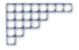
Figure 1. Diagram of the partition $\lambda=(8,5,4,2,1)$.

Let $\mathscr{V}=\chi(\mathscr{O}_{Z})$ denote the tautological rank $n$ vector bundle over $\operatorname{Hilb}(\mathbb{C}^{2},n)$ as in Section 3.2.7, and let

$$V_{\lambda} =\chi(\mathscr{O}_{Z_{\lambda}})$$

(98) $$=\sum_{(i,j)\in\lambda}t_{1}^{-i}t_{2}^{-j}$$

be the character of its stalk at $I_{\lambda}$. Clearly, this is nothing but the generating function for the diagram $\lambda$. From (95) and (97) we deduce the following

Proposition 99.

Let $I_{\lambda}\subset\mathbb{C}[x_{1},x_{2}]$ be a monomial ideal and let $V$ denote the generating function (98) for the diagram of $\lambda$. We have

(100) $$T_{I_{\lambda}}\operatorname{Hilb}=V+\overline{V}\,t_{1}t_{2}-V\overline{V}\,(1-t_{1})(1-t_{2})\,.$$

as a $T$-module, where $\overline{V}=V^{*}$ denotes the dual.

For example, take

$$\lambda=\square\,,\quad I_{\lambda}=\mathsf{m}=(x_{1},x_{2})\,,\quad V=1$$

then

$$T_{\square}\operatorname{Hilb}=1+t_{1}t_{2}-(1-t_{1})(1-t_{2})=t_{1}+t_{2}=\mathbb{C}^{2}$$

in agreement with $\operatorname{Hilb}(X,1)\cong X$.

3.4.5.

Formula (100) may be given the following combinatorial polish. For a square $\square=(i,j)$ in the diagram of $\lambda$ define its arm-length and leg-length by

$$a(\square) = \#\{j^{\prime}>j\, \big{|}\,(i,j^{\prime})\in\lambda\}\,,$$

(101) $$l(\square) = \#\{i^{\prime}>i\, \big{|}\,(i^{\prime},j)\in\lambda\}\,,$$

see Figure 2.

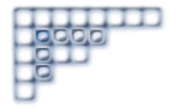
Figure 2. For the box $\square=(1,1)$ in this diagram, we have $a(\square)=3$ and $l(\square)=2$.

Exercise 102.

Prove that

(103) $$T_{I_{\lambda}}\operatorname{Hilb}=\sum_{\square\in\lambda}t_{1}^{-l(\square)}t_{2}^{a(\square)+1}+t_{1}^{l(\square)+1}t_{2}^{-a(\square)}\,.$$

Exercise 104.

Prove a generalization of (100) and (103) for the character of $\chi(\mathscr{O}_{X})-\chi(I_{\lambda},I_{\mu})$. If in need of a hint, open [CO].

Exercise 105.

Using the formulas for $T_{I_{\lambda}}\operatorname{Hilb}$ and equivariant localization, write a code for the computation of the series

$$\mathsf{Z}_{\operatorname{Hilb}(\mathbb{C}^{2})}=\sum_{n,i\geq 0}z^{n}(-m)^{i}\,\chi(\operatorname{Hilb}(\mathbb{C}^{2},n),\Omega^{i})$$

and check experimentally that is ${\mathsf{S}}^{\raisebox{1.42262pt}{$\scriptscriptstyle\bullet$}}$ of a nice rational function of the variables $z,m,t_{1},t_{2}$. We will compute this function theoretically in Section 5.3.4.

3.4.6.

We now advance to the discussion of the case when $X$ is a nonsingular threefold and $Z\subset X$ is a $1$-dimensional subscheme and $\mathscr{I}_{Z}$ is its sheaf of ideals. The sheaf $\mathscr{I}_{Z}$ is clearly torsion-free, as a subsheaf of $\mathscr{O}_{X}$, and

$$\det\mathscr{I}_{Z}=\mathscr{O}_{X}$$

because the two sheaves differ in codimension $\geq 2$.

Donaldson-Thomas theory views $\operatorname{Hilb}(X,\textup{curves})$ as the moduli space of torsion-free sheaves rank 1 sheaves $\mathscr{I}$ with trivial determinant. For any such sheaf we have

$$\mathscr{I}\hookrightarrow\mathscr{I}^{\vee\vee}=\det\mathscr{I}=\mathscr{O}_{X}$$

and so $\mathscr{I}$ is the ideal sheaf of a subscheme $Z\subset X$. We have

$$0=c_{1}(\det\mathscr{I})=c_{1}(\mathscr{I})=[Z]\in H_{4}(X,\mathbb{Z})$$

and therefore $\dim Z=1$. The deformation theory of sheaves gives

$$T^{\textup{vir}}_{\mathscr{I}}\operatorname{Hilb}=\operatorname{Def}(\mathscr{I})-\operatorname{Obs}(\mathscr{I}) =\chi(\mathscr{O}_{X})-\chi(\mathscr{I},\mathscr{I})\,,$$

(106) $$=\chi(\mathscr{O}_{Z})+\chi(\mathscr{O}_{Z},\mathscr{O}_{X})-\chi(\mathscr{O}_{Z},\mathscr{O}_{Z})$$

just like in Proposition 94.

The group $\operatorname{Ext}^{1}(\mathscr{I},\mathscr{I})$ which enters (106) parametrizes sheaves on $B\times X$ flat over $B$ for $B=\mathbb{C}[\varepsilon]/\varepsilon^{2}$, just like in Exercise 89. It describes the deformations of the sheaf $\mathscr{I}$. The obstructions to these deformations lie in $\operatorname{Ext}^{2}(\mathscr{I},\mathscr{I})$.

We now examine how this works for the Hilbert scheme of points in $\mathbb{C}^{3}$.

3.4.7.

Let $\pi$ be a 3-dimensional partition and let $I_{\pi}\subset\mathbb{C}[x_{1},x_{2},x_{3}]$ be the corresponding monomial ideal. The passage from (95) to (100) is exactly the same as before, with the correction for

$$\chi(\mathscr{O}_{\mathbb{C}^{3}})=\frac{1}{(1-t_{1}^{-1})(1-t_{2}^{-1})(1-t_{3}^{-1})}\,.$$

We obtain the following

Proposition 107.

Let $I_{\pi}\subset\mathbb{C}[x_{1},x_{2},x_{3}]$ be a monomial ideal and let $V$ denote the generating function for $\pi$, that is, the character of $\mathscr{O}_{Z_{\pi}}$. We have

(108) $$T_{I_{\pi}}^{\textup{vir}}\operatorname{Hilb}=V-\overline{V}\,t_{1}t_{2}t_{3}-V\overline{V}\,\prod_{1}^{3}(1-t_{i})\,.$$

as a $T$-module.

As an example, take

$$\pi=\textup{\char 114}\,,\quad I_{\pi}=\mathsf{m}=(x_{1},x_{2},x_{2})\,,\quad V=1$$

then

$$T^{\textup{vir}}_{\textup{\char 114}}\operatorname{Hilb}=t_{1}+t_{2}+t_{3}-t_{1}t_{2}-t_{1}t_{3}-t_{2}t_{3}=\mathbb{C}^{3}-\det\mathbb{C}^{3}\otimes\left(\mathbb{C}^{3}\right)^{*}$$

in agreement with the identification

$$\mathbb{M}(1)=\operatorname{Hilb}(X,1)\cong X\cong\operatorname{Hilb}(\mathsf{Free}_{3},1)={\widetilde{\mathbb{M}}}(1)$$

for the Hilbert schemes of $1$ point in $X=\mathbb{C}^{3}$ and the description of the obstruction bundle as

$$\operatorname{Obs}=\boldsymbol{\kappa}\otimes T^{*}_{{\widetilde{\mathbb{M}}}}=\boldsymbol{\kappa}\otimes\left(\mathbb{C}^{3}\right)^{*}$$

where $\boldsymbol{\kappa}=\det\mathbb{C}^{3}$.

In general, for ${\widetilde{\mathbb{M}}}=\operatorname{Hilb}(\mathsf{Free}_{3},n)$ we have

$$T_{\widetilde{\mathbb{M}}}=(\mathbb{C}^{3}-1)\otimes\overline{V}\otimes V+V$$

by the construction of ${\widetilde{\mathbb{M}}}$ as the space of 3 operators and a vector in $V$ modulo the action of $GL(V)$. Therefore

$$T^{\textup{vir}} =T_{\widetilde{\mathbb{M}}}-\boldsymbol{\kappa}^{-1}\otimes T^{*}_{{\widetilde{\mathbb{M}}}}$$

(109) $$=V-\det\mathbb{C}^{3}\otimes\overline{V}-\overline{V}\otimes{V}\otimes\sum(-1)^{i}\Lambda^{i}\mathbb{C}^{3}\,,$$

which gives a different and more direct proof of (108).

Exercise 110.

$\dots$ or, rather, a combinatorial challenge. Is there a combinatorial formula for the character of $T_{\widetilde{\mathbb{M}}}$ at torus-fixed points and can one find some systematic cancellations in the first line of (109) ?

3.4.8.

Let

$$\tilde{\iota}:\mathbb{M}\hookrightarrow{\widetilde{\mathbb{M}}}$$

be the inclusion of $\mathbb{M}=\operatorname{Hilb}(\mathbb{C}^{3},\textup{points})$ into the Hilbert scheme of a free algebra. By our earlier discussion,

$$\tilde{\iota}_{*}\mathscr{O}^{\textup{vir}}={\Lambda}^{\!\raisebox{1.42262pt}{$\scriptscriptstyle\bullet$}}\!\operatorname{Obs}^{*}$$

and therefore we can use equivariant localization on the smooth ambient space ${\widetilde{\mathbb{M}}}$ to compute $\chi(\mathbb{M},\mathscr{O}^{\textup{vir}})$.

Let $\pi$ be 3-dimensional partition and $I_{\pi}\in\operatorname{Hilb}\subset{\widetilde{\mathbb{M}}}$ the corresponding fixed point. Since

$$T^{\textup{vir}}_{\pi}=T_{\pi}{\widetilde{\mathbb{M}}}-\boldsymbol{\kappa}\otimes\left(T_{\pi}{\widetilde{\mathbb{M}}}\right)^{*}\,,$$

we have

$$T^{\textup{vir}}_{\pi}=\sum_{w}\left(w-\frac{\boldsymbol{\kappa}}{w}\right)$$

where the sum is over the weights $w$ of $T_{\pi}{\widetilde{\mathbb{M}}}$. Therefore

(111) $$\mathscr{O}^{\textup{vir}}_{\operatorname{Hilb}(\mathbb{C}^{3},n)}=\sum_{|\pi|=n}\mathscr{O}_{I_{\pi}}\prod\frac{1-w/\boldsymbol{\kappa}}{1-w^{-1}}$$

in localized equivariant K-theory. This formula illustrates a very important notion of virtual localization, see in particular [GP, FG, CF3], which we now discuss.

3.4.9.

Let a torus $T$ act on a scheme $\mathbb{M}$ with a $T$-equivariant perfect obstruction theory. For example, $\mathbb{M}$ be DT moduli space for a nonsingular threefold $X$ on which a torus $T$ act. Let $\mathbb{M}^{T}\subset\mathbb{M}$ be the subscheme of fixed points. We can decompose

$$\left(\operatorname{Def}-\operatorname{Obs}\right)|_{\mathbb{M}^{T}}= \,\operatorname{Def}^{\textup{fixed}}-\operatorname{Obs}^{\textup{fixed}}$$

(112) $$+ \,\operatorname{Def}^{\textup{moving}}-\operatorname{Obs}^{\textup{moving}}$$

in which the fixed part is formed by trivial $T$-modules and the moving part by nontrivial ones.

Exercise 113.

Check that for $\operatorname{Hilb}(\mathbb{C}^{3},\textup{points})$ and the maximal torus $T\subset GL(3)$ the fixed part of the obstruction theory vanishes.

By a result of [GP], the fixed part of the obstruction theory is perfect obstruction theory for $\mathbb{M}^{T}$ and defines $\mathscr{O}^{\textup{vir}}_{\mathbb{M}^{T}}$. The virtual localization theorem of [CF3], see also [GP] for a cohomological version, states that

(114) $$\mathscr{O}^{\textup{vir}}_{\mathbb{M}}=\iota_{*}\left(\mathscr{O}^{\textup{vir}}_{\mathbb{M}^{T}}\otimes{\mathsf{S}}^{\raisebox{1.42262pt}{$\scriptscriptstyle\bullet$}}\left(\operatorname{Def}^{\textup{moving}}-\operatorname{Obs}^{\textup{moving}}\right)^{*}\right)$$

where

$$\iota:\mathbb{M}^{T}\hookrightarrow\mathbb{M}$$

is the inclusion. Since, by construction, the moving part of the obstruction theory contains only nonzero $T$-weights, its symmetric algebra ${\mathsf{S}}^{\raisebox{1.42262pt}{$\scriptscriptstyle\bullet$}}$ is well defined.

Exercise 115.

Let $f(\mathscr{V})$ be a Schur functor of the tautological bundle $\mathscr{V}$ over $\operatorname{Hilb}(\mathbb{C}^{3},n)$, for example

$$f(\mathscr{V})=S^{2}\mathscr{V},\Lambda^{3}\mathscr{V},\dots\,.$$

Write a localization formula for $\chi(\operatorname{Hilb}(\mathbb{C}^{3},n),\mathscr{O}^{\textup{vir}}\otimes f(\mathscr{V}))$.

3.4.10.

It remains to twist (111) by

$$\mathscr{K}_{\textup{vir}}^{1/2}={\det}^{-1/2}\,T^{\textup{vir}}$$

to deduce a virtual localization formula for $\widehat{\mathscr{O}}^{\textup{vir}}$. It is convenient to define the transformation $\widehat{\mathsf{a}}(\dots)$, a version of the $\widehat{A}$-genus, by

$$\widehat{\mathsf{a}}(x+y)=\widehat{\mathsf{a}}(x)\,\widehat{\mathsf{a}}(y)\,,\quad\widehat{\mathsf{a}}(w)=\frac{1}{w^{1/2}-w^{-1/2}}$$

where $w$ is a monomial, that is, a weight of $T$. For example

(116) $$\widehat{\mathsf{a}}\left(T^{\textup{vir}}_{\pi}\right)=\prod_{w}\frac{(\boldsymbol{\kappa}/w)^{1/2}-(w/\boldsymbol{\kappa})^{1/2}}{w^{1/2}-w^{-1/2}}\,,$$

where the product is over the same weights $w$ as in (111).

With this notation, we can state the following

Proposition 117.

We have

(118) $$\widehat{\mathscr{O}}^{\textup{vir}}_{\operatorname{Hilb}(\mathbb{C}^{3},n)}=(-1)^{n}\,\sum_{|\pi|=n}\widehat{\mathsf{a}}\left(T^{\textup{vir}}_{\pi}\right)\,\mathscr{O}_{I_{\pi}}$$

in localized equivariant K-theory.

Exercise 119.

Write a code to check a few first terms in $z$ of Nekrasov’s formula (75).

Exercise 120.

Take the limit $t_{1},t_{2},t_{3}\to 1$ in Nekrasov’s formula for $\mathbb{C}^{3}$ and show that it correctly reproduces the formula for $\mathsf{Z}_{\mathbb{C}^{3},\textup{points},\textup{coh}}$ from Theorem 87.

3.5. Proof of Nekrasov’s formula

3.5.1.

Our next goal is to prove Nekrasov’s formula for $X=\mathbb{C}^{3}$. By localization, this immediately generalizes to nonsingular toric threefolds. Later, when we discuss relative invariants, we will see the generalization to the relative setting. The path from there to general threefolds is the same as in [LevPand].

Our proof of Theorem (74) will have two parts. In the first step, we prove

(121) $$\mathsf{Z}_{\mathbb{C}^{3},\textup{points}}={\mathsf{S}}^{\raisebox{1.42262pt}{$\scriptscriptstyle\bullet$}}\frac{\star}{(1-t_{1}^{-1})(1-t_{2}^{-1})(1-t_{3}^{-1})}$$

where

$$\star\in\mathbb{Z}\left[t_{1}^{\pm 1},t_{2}^{\pm 1},t_{3}^{\pm 1},(t_{1}t_{2}t_{3})^{1/2}\right][[z]]$$

is a formal power series in $z$, without a constant term, with coefficients in Laurent polynomials. In the second step, we identify the series $\star$ by a combinatorial argument involving equivariant localization.

The first step is geometric and, in fact, we prove that

(122) $$\mathsf{Z}_{\mathbb{C}^{3},\textup{points}}={\mathsf{S}}^{\raisebox{1.42262pt}{$\scriptscriptstyle\bullet$}}\chi(\mathbb{C}^{3},\mathscr{G})\,,\quad\mathscr{G}=\sum_{i=1}^{\infty}z^{i}\,\mathscr{G}_{i}\,,\quad\mathscr{G}_{i}\in K_{GL(3)}(\mathbb{C}^{3})\,,$$

where each $\mathscr{G}_{i}$ is constructed iteratively starting from

$$\mathscr{G}_{1}=-\widehat{\mathscr{O}}^{\textup{vir}}_{\operatorname{Hilb}(\mathbb{C},1)}\,.$$

The same argument applies to many similar sheaves and moduli spaces, including, for example, the generating function

(123) $$\sum_{n}z^{n}\chi(\operatorname{Hilb}(\mathbb{C}^{3},n),\mathscr{O}^{\textup{vir}})$$

in which we have $z^{n}$ instead of $(-z)^{n}$ and plain $\mathscr{O}^{\textup{vir}}$ instead of the symmetrized virtual structure sheaf. The second part of the proof, however, doesn’t work for $\mathscr{O}^{\textup{vir}}$ and I don’t know a reasonable formula for the series (123).

It is natural to prove (122) in that greater generality and this will be done in Proposition 196 in Section 5.3.5 below. For now, we assume (122) and proceed to the second part of the proof, that is, to the identification of the polynomial $\star$ in (121).

3.5.2.

For $\operatorname{Hilb}(\mathbb{C}^{3},n)$, the line bundles $\mathscr{L}_{4}$ and $\mathscr{L}_{5}$ in (68) are necessarily trivial with, perhaps, a nontrivial equivariant weight. Hence the determinant term in (68) is a trivial bundle with weight

(124) $${\det}^{1/2}\pi_{\mathbb{M},*}(\mathfrak{F}\otimes(\mathscr{L}_{4}-\mathscr{L}_{5}))=\left(\frac{\textup{weight}(\mathscr{L}_{4})}{\textup{weight}(\mathscr{L}_{5})}\right)^{n/2}\,,$$

which can be absorbed in the variable $z$. Therefore, without loss of generality, we can assume that

$$\mathscr{L}_{4}=\mathscr{L}_{5}=\boldsymbol{\kappa}^{-1/2}=\frac{1}{(t_{1}t_{2}t_{3})^{1/2}}\,,$$

where $t_{i}$’s are the weights of the $GL(3)$ action on $\mathbb{C}^{3}$, in which case the term (124) is absent.

We define

$$t_{4}=\frac{z}{\boldsymbol{\kappa}^{1/2}}\,,\quad t_{5}=\frac{1}{z\,\boldsymbol{\kappa}^{1/2}}\,,$$

so that $t_{1},\dots,t_{5}$ may be interpreted as the weights of the action of $SL(5)\supset\mathbb{C}^{\times}_{z}$ on $Z\cong\mathbb{C}^{5}$. With this notation, what needs to be proven is

$$\mathsf{Z}_{\mathbb{C}^{3},\textup{points}} ={\mathsf{S}}^{\raisebox{1.42262pt}{$\scriptscriptstyle\bullet$}}\,\,\widehat{\mathsf{a}}\left(\sum_{i=1}^{5}t_{i}-\sum_{i<j\leq 3}t_{i}t_{j}\right)$$

(125) $$={\mathsf{S}}^{\raisebox{1.42262pt}{$\scriptscriptstyle\bullet$}}\,\frac{\prod_{i<j\leq 3}((t_{i}t_{j})^{1/2}-(t_{i}t_{j})^{-1/2})}{\prod_{i\leq 5}(t_{i}^{1/2}-t_{i}^{-1/2})}\,.$$

3.5.3.

Exercise 126.

Prove that the localization weight (116) of any nonempty 3-dimensional partition is divisible by $t_{1}t_{2}-1$. In fact, the order of vanishing of this weight at $t_{1}t_{2}=1$ is computed in Section 4.5 of [OP2].

By symmetry, the same is clearly true for all $t_{i}t_{j}-1$ with $i<j\leq 3$. Note that plethystic substitutions $\{t_{i}\}\mapsto\{t_{i}^{k}\}$ preserve vanishing at $t_{i}t_{j}=1$. Therefore, using (121), we may define

$$\textup{\char 73}\in\mathbb{Z}[t_{1}^{\pm 1/2},t_{2}^{\pm 1/2},t_{3}^{\pm 1/2}][[z]]$$

so that

(127) $$\mathsf{Z}_{\mathbb{C}^{3},\textup{points}}={\mathsf{S}}^{\raisebox{1.42262pt}{$\scriptscriptstyle\bullet$}}\,\left(\textup{\char 73}\,\prod_{i=1}^{3}\frac{(\boldsymbol{\kappa}/t_{i})^{1/2}-(t_{i}/\boldsymbol{\kappa})^{1/2}}{t_{i}^{1/2}-t_{i}^{-1/2}}\right)\,.$$

Proposition 128.

We have

$$\textup{\char 73}\in\mathbb{Z}[\boldsymbol{\kappa}^{\pm 1}][[z]]\,,$$

that is, this polynomial depends only on the product $t_{1}t_{2}t_{3}$, and not on the individual $t_{i}$’s.

Proof.

A fraction of the form

$$\frac{(\boldsymbol{\kappa}/w)^{1/2}-(w/\boldsymbol{\kappa})^{1/2}}{w^{1/2}-w^{-1/2}}$$

remains bounded and nonzero as $w^{\pm 1}\to\infty$ with $\boldsymbol{\kappa}$ fixed. Therefore, both the localization contributions (116) and the fraction in (127) remain bounded as $t_{i}^{\pm 1}\to\infty$ in such a way that $\boldsymbol{\kappa}$ remains fixed. We conclude that the Laurent polynomial ✩ is bounded at all such infinities and this means it depends on $\boldsymbol{\kappa}$ only. ∎

This is our first real example of rigidity.

3.5.4.

The proof of Nekrasov’s formula for $\mathbb{C}^{3}$ will be complete if we show the following

Proposition 129.

$$\textup{\char 73}=\frac{1}{(t_{4}^{1/2}-t_{4}^{-1/2})(t_{5}^{1/2}-t_{5}^{-1/2})}=-\frac{z}{(1-\boldsymbol{\kappa}^{1/2}\,z)(1-\boldsymbol{\kappa}^{-1/2}\,z)}$$

To compute ✩, we may let the variables $t_{i}$ go to infinity with $\boldsymbol{\kappa}$ fixed. Since

$$\frac{(\boldsymbol{\kappa}/w)^{1/2}-(w/\boldsymbol{\kappa})^{1/2}}{w^{1/2}-w^{-1/2}}\to\begin{cases}-\boldsymbol{\kappa}^{-1/2}\,,&w\to\infty\,,\\ -\boldsymbol{\kappa}^{1/2}\,,&w\to 0\,,\end{cases}$$

we conclude that

$$\widehat{\mathsf{a}}\left(\sum w_{i}-\boldsymbol{\kappa}\sum w_{i}^{-1}\right)\to(-\boldsymbol{\kappa}^{1/2})^{\operatorname{index}}$$

where

$$\operatorname{index}=\#\left\{i\,\big{|}\,w_{i}\to 0\right\}-\#\left\{i\,\big{|}\,w_{i}\to\infty\right\}\,.$$

For the computation of ✩ we are free to send $t_{i}$ to infinity in any way we like, as long as their product stays fixed. As we will see, a particularly nice choice is

(130) $$t_{1},t_{3}\to 0\,,\quad|t_{1}|\ll|t_{3}|\,,\quad\boldsymbol{\kappa}=\textup{fixed}\,.$$

For the fraction in (127) we have

$$\prod_{i=1}^{3}\frac{(\boldsymbol{\kappa}/t_{i})^{1/2}-(t_{i}/\boldsymbol{\kappa})^{1/2}}{t_{i}^{1/2}-t_{i}^{-1/2}}\to(-\boldsymbol{\kappa}^{1/2})^{\operatorname{index}(\mathbb{C}^{3})}=-\boldsymbol{\kappa}^{1/2}\,.$$

Thus Proposition 129 becomes a corollary of the following

Proposition 131.

Let the variables $t_{i}$ go to infinity of the torus as in (130). Then

(132) $$\mathsf{Z}_{X,\textup{points}}\to{\mathsf{S}}^{\raisebox{1.42262pt}{$\scriptscriptstyle\bullet$}}\,\frac{\boldsymbol{\kappa}^{1/2}\,z}{(1-\boldsymbol{\kappa}^{1/2}\,z)(1-\boldsymbol{\kappa}^{-1/2}\,z)}\,.$$

This is a special case of the computations of index vertices from Section 7 of [67] and the special case of the limit (130) corresponds to the refined vertex of Iqbal, Kozcaz, and Vafa in [IKV]. We will now show how this works in the example at hand.

3.5.5.

Recall the formula

$$T_{I_{\pi}}{\widetilde{\mathbb{M}}}=(\mathbb{C}^{3}-1)\otimes\overline{V}\otimes V+V$$

for tangent space to ${\widetilde{\mathbb{M}}}$ at a point corresponding to a 3-dimensional partition $\pi$ with the generating function $V$. For a partition of size $n$, this is a sum of $2n^{2}+n$ terms and, in principle, we need to compute the index of this very large torus module to know the asymptotics of $\widehat{\mathsf{a}}(T^{\textup{vir}}_{\pi})$ as $t\to\infty$.

A special feature of the limit (130) is that one can see a cancellation of $2n^{2}$ terms in the index, with the following result

Lemma 133.

In the limit (130),

$$\operatorname{index}\left(T_{I_{\pi}}{\widetilde{\mathbb{M}}}\right)=\operatorname{index}\left(t_{3}^{k}\,V\right)\,,$$

for any $k$ is such that $k>|\pi|$ but $|t_{1}|\ll|t_{3}|^{k}$.

This Lemma is proven in the Appendix to [67]. Clearly

$$\operatorname{index}\left(t_{3}^{k}\,V\right)=\sum_{\textup{\char 114}=(i_{1},i_{2},i_{3})\in\pi}\textup{sgn}\,(i_{2}-i_{1}+0)$$

and therefore Proposition 131 becomes the

$$z\boldsymbol{\kappa}^{1/2} =q_{0}=q_{1}=q_{2}=\dots$$

(134) $$z\boldsymbol{\kappa}^{-1/2} =q_{-1}=q_{-2}=\dots$$

case of the following generalization of McMahon’s enumeration

Theorem 135 ([OR1, OR2]).

(136) $$\sum_{\pi}\prod_{\textup{\char 114}=(i_{1},i_{2},i_{3})\in\pi}q_{i_{2}-i_{1}}={\mathsf{S}}^{\raisebox{1.42262pt}{$\scriptscriptstyle\bullet$}}\sum_{a\leq 0\leq b}q_{a}q_{a+1}\cdots q_{b-1}q_{b}$$

With the specialization (134) the sum under ${\mathsf{S}}^{\raisebox{1.42262pt}{$\scriptscriptstyle\bullet$}}$ in (136) become the series expansion of the fraction in (132).

3.5.6.

We conclude with a sequence of exercises that will lead the reader through the proof of Theorem 135. It is based on introducing a transfer matrix, a very much tried-and-true tool in statistical mechanics and combinatorics.

A textbook example of transfer matrix arises in 2-dimensional Ising model on a torus. The configuration space in that model are assignments of $\pm 1$ spins to sites $x$ of a rectangular grid, that is, functions

$$\sigma:\{1,\dots,M\}\times\{1,\dots,N\}\to\{\pm 1\}$$

Each is weighted with

$$\operatorname{Prob}(\sigma)\propto W(\sigma)=\exp(-\beta E(\sigma))\,,$$

where $\beta$ is the inverse temperature and the energy $E$ is defined by

$$E(\sigma)=-\sum_{\textup{nearest neighbors $x$ and $x^{\prime}$}}\sigma(x)\sigma(x^{\prime})\,,$$

with periodic boundary conditions.

Now introduce a vector space

$$V\cong(\mathbb{C}^{2})^{N}$$

with a basis formed by all possible spin configurations $\vec{\sigma}$ in one column of our grid. Define a diagonal matrix $\mathsf{W}^{\textup{v}}$ and a dense matrix $\mathsf{W}^{\textup{h}}$ by

(137) $$\mathsf{W}^{\textup{v}}_{\vec{\sigma},\vec{\sigma}} =\exp\left(-\beta\sum_{\begin{subarray}{c}\textup{vertical neighbors}\\ \textup{ in column $\vec{\sigma}$}\end{subarray}}\sigma(x)\,\sigma(x^{\prime})\right)$$

(138) $$\mathsf{W}^{\textup{h}}_{\vec{\sigma}_{1},\vec{\sigma}_{2}} =\exp\left(-\beta\sum_{\begin{subarray}{c}\textup{horizontal neighbors}\\ \textup{ in columns $\vec{\sigma}_{1}$ and $\vec{\sigma}_{2}$ }\end{subarray}}\sigma_{1}(x)\,\sigma_{2}(x^{\prime})\right)\,,$$

see Figure 3.

Exercise 139.

Prove that

$$\sum_{\{\sigma\}}W(\sigma)=\operatorname{tr}\,(\mathsf{W}^{\textup{v}}\mathsf{W}^{\textup{h}})^{M}$$

where the summation is over all $2^{MN}$ spin configurations $\{\sigma\}$.

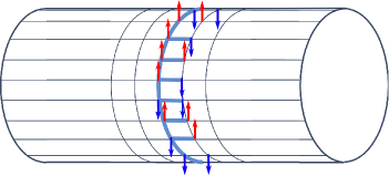
Figure 3. The transfer matrix $\mathsf{W}^{\textup{v}}\mathsf{W}^{\textup{h}}$ of the Ising model captures the interactions of the spins in two adjacent columns along the highlighted edges. Iterations of the transfer matrix cover all spins and all edges.

The matrix $\mathsf{W}^{\textup{v}}\mathsf{W}^{\textup{h}}$ is an example of a transfer matrix. Onsager’s great discovery was the diagonalization of this matrix. Essentially, he has shown that the transfer matrix is in the image of a certain matrix $g\in O(2N)$ in the spinor representation of this group.

3.5.7.

Now in place of the spinor representation of $O(2N)$ we will have the action of the Heisenberg algebra $\widehat{\mathfrak{gl}}(1)$ on

$$V=\textup{Fock space}=\textup{symmetric functions}=\\ =\textup{polynomial representations of $GL(\infty)$}\,.$$

This space has an orthonormal basis $\{s_{\lambda}\}$ of Schur functions, that is, the characters of the Schur functors $S^{\lambda}\mathbb{C}^{\infty}$ of the defining representation of $GL(\infty)$. It is indexed by 2-dimensional partitions $\lambda$ which will arise as slices of $3$-dimensional partitions $\pi$ by planes $i_{2}-i_{1}=\textup{const}$.

The diagonal operator $\mathsf{W}^{\textup{v}}$ will be replaced by the operator

$$q^{|\,\cdot\,|}\,s_{\lambda}=q^{|\lambda|}s_{\lambda}\,.$$

In place of the nondiagonal operator $\mathsf{W}^{\textup{h}}$, we will use the operators

$$\Gamma_{-}(z)=\left(\sum_{k\geq 0}z^{k}\,\mathsf{S}^{k}\mathbb{C}^{\infty}\right)\otimes$$

and its transpose $\Gamma_{+}$. The character of $\mathsf{S}^{k}\mathbb{C}^{\infty}$ is the Schur function $s_{k}$. It is well known that

$$\Gamma_{-}(z)\,s_{\lambda}=\sum_{\mu}z^{|\mu|-|\lambda|}\,s_{\mu}$$

where the summation is over all partitions $\mu$ such that $\mu$ and $\lambda$ interlace, which means that

$$\mu_{1}\geq\lambda_{1}\geq\mu_{2}\geq\lambda_{2}\geq\dots\,.$$

Exercise 140.

Prove that

$$\sum_{\pi}\prod_{\textup{\char 114}=(i_{1},i_{2},i_{3})\in\pi}q_{i_{2}-i_{1}}=\\ =\left(\cdots\Gamma_{+}(1)\,q_{-1}^{|\,\cdot\,|}\,\Gamma_{+}(1)\,q_{0}^{|\,\cdot\,|}\,\Gamma_{-}(1)\,q_{1}^{|\,\cdot\,|}\,\Gamma_{-}(1)\,q_{2}^{|\,\cdot\,|}\cdots s_{\varnothing},s_{\varnothing}\right)\,.$$

Exercise 141.

Prove that $q^{|\,\cdot\,|}\,\Gamma_{-}(z)=\Gamma_{-}(qz)\,q^{|\,\cdot\,|}$ and that

$$\Gamma_{+}(z)\,\Gamma_{-}(w)=\frac{1}{1-zw}\Gamma_{-}(w)\,\Gamma_{+}(z)$$

if $|zw|<1$. Deduce Theorem 135.

3.5.8.

Ultimately, the idea of transfer matrix rests on certain fundamental principles of mathematical physics which may be applied both in the discrete and continuous situations.

The first such principle is gluing local field theories, which in the discrete situation means the following. Suppose we want to compute a partition function of the form

$$Z=\sum_{\phi\in\Phi^{\Omega}}e^{-E(\phi)}$$

where $\Omega$ is a graph, $\Phi^{\Omega}$ is the space of functions

$$\phi:\Omega\to\Phi$$

and

$$E(\phi)=\sum_{x,y\in\Omega}V_{2}(x,y,\phi(x),\phi(y))+\sum_{x\in\Omega}V_{1}(x,\phi(x))\,.$$

For example, for the Ising model we have $\Phi=\{\pm 1\}$,

$$V_{2}(x,y,\phi(x),\phi(y))=\begin{cases}-\beta\phi(x)\phi(y)\,,\quad&\textup{$x$ and $y$ are neighbors}\,,\\ 0&\textup{otherwise}\,,\end{cases}$$

and $V_{1}=0$ if there is no external magnetic field.

Suppose the pair potential $V_{2}$ has finite range, that is, suppose there exists a constant $R$ such that

$$\operatorname{distance}(x,y)>R\Rightarrow V_{2}(x,y,\dots)=0\,.$$

For example, for the Ising model $R=1$. Suppose

$$\Omega=\Omega_{1}\sqcup B\sqcup\Omega_{2}$$

where the boundary region $B$ disconnects $\Omega_{1}$ from $\Omega_{2}$ in the sense that

$$\operatorname{distance}(\Omega_{1},\Omega_{2})>R$$

as in Figure 4. Then

(142) $$Z=\sum_{\phi_{B}\in\Phi^{B}}e^{-E(\phi_{B})}\,Z(\Omega_{1}\big{|}\phi_{B})\,Z(\Omega_{2}\big{|}\phi_{B})\,,$$

where the partition functions $Z(\Omega_{1}\big{|}\phi_{B})$ with boundary conditions imposed on $B$ are defined by

$$Z(\Omega_{i}\big{|}\phi_{B})=\sum_{\phi_{\Omega_{i}}\in\Phi^{\Omega_{i}}}e^{-E(\phi_{\Omega_{i}})-E(\phi_{\Omega_{i}}\big{|}\phi_{B})}$$

with

$$E(\phi_{\Omega_{i}}\big{|}\phi_{B})=\sum_{x\in\Omega_{i},y\in B}V_{2}(x,y,\phi(x),\phi(y))\,.$$

Effectively, fixing the boundary conditions on $B$ modifies the 1-particle potential $V_{1}$ in an tube of radius $R$ around $B$.

If $V_{1}$ and $V_{2}$ are real, then clearly (142) may be written as

$$Z=\Big{(}Z(\Omega_{1}\big{|}\,\cdot\,),Z(\Omega_{2}\big{|}\,\cdot\,)\Big{)}_{L^{2}(\Phi^{B},e^{-E(\phi_{B})})}\,.$$

In any event, it may be more prudent to interpret (142) as a pairing between a pair of dual vector spaces, as in the continuous limit the two partition functions paired in (142) may turn out to be objects of rather different nature. In this very abstract form, gluing says that if $B$ disconnects $\Omega$, then partition functions $Z(\Omega_{1}\big{|}\,\cdot\,)$ give a pair of vectors in dual vector spaces so that

(143) $$Z=\left\langle Z(\Omega_{1}\big{|}\,\cdot\,),Z(\Omega_{2}\big{|}\,\cdot\,)\right\rangle\,.$$

This is probably very familiar to most readers from TQFT context, but is not restricted to topological theories.

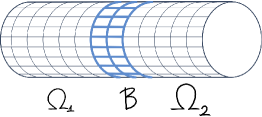
Figure 4. If the domain $\Omega$ is glued from two pieces then the partition function is a pairing of a vector and a covector.

The second principle on which transfer matrices rest is that if $B$ itself is disconnected

$$B=B_{1}\sqcup B_{2}\,,\quad\operatorname{distance}(B_{1},B_{2})>R\,,$$

then

$$L^{2}(\Phi^{B})=L^{2}(\Phi^{B_{1}})\otimes L^{2}(\Phi^{B_{2}})\,,$$

as inner product spaces. Again, in continuous limit, it may be better to talk about operators from one functional space to another — the transfer matrix, or the evolution operator. Multiplying such operators, we can build larger domains from small pieces (e.g. a long cylinder from a short one) like we did in the two examples above.

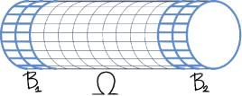
Figure 5. If the boundary has two components then the partition function is an operator.

A larger supply of operators may be obtained by modifying the partition function $Z(\Omega\big{|}B_{1}\cup B_{2})$ by, for example, inserting a local observable.

3.5.9.

The purpose of this abstract discussion of transfer matrices is that our goals in these notes may be directly compared to understanding the transfer matrix of the Ising model or 3-dimensional partitions in terms of representation theory of a certain algebra.

For a mathematical physicist, the study of quasimaps to Nakajima varieties appears as a low energy limit in the study of supersymmetric gauge theories. A gauge theory is specified by a choice of a gauge group $G$ and a representation in which the matter fields of theory transform. If the choices are made like in the next section, then a Nakajima variety $X$ appears as the one of the components (the Higgs branch) of the moduli spaces of vacua. In the low energy limit (also known as the thermodynamic, or infrared limit), the state of the system is described as a modulated vacuum state, or as a map from the spacetime to the moduli spaces of vacua.

K-theory of quasimaps $f:C\dasharrow X$, where $C$ is a Riemann surface, is relevant for the study of 3-dimensional supersymmetric gauge theories on manifold of the form $C\times S^{1}$. General ideas about cutting and gluing apply to the surface $C$. In particular, $K(X)$ will be the vector space associated to a puncture in $C$ and various vectors and operators in this space that will occupy us below may be interpreted as partition functions with given boundary conditions. The eventual goal will be to understand these operators in terms of representation theory of a certain quantum loop algebra $\mathscr{U}_{\hbar}(\hat{\mathfrak{g}})$ acting on $K(X)$, see Sections 9, 10, and [75].

This quantum loop algebra action extends the actions constructed by Nakajima [Nak3]. Nekrasov and Shatashvili [NS1, NS2] were the first to realize this connection between supersymmetric gauge theories, quantum integrable systems, and Nakajima theory.

4. Nakajima varieties

4.1. Algebraic symplectic reduction

4.1.1.

Symplectic reduction was invented in classical mechanics [ArnMech] to deal with the following situation. Let $M$ be the configuration space of a mechanical system and $T^{*}M$ — the corresponding phase space. A function $H$, called Hamiltonian, generates dynamics by

$$\frac{d}{dt}f=\{H,f\}$$

where $f$ is an arbitrary function on $T^{*}M$ and $\{\,\cdot\,,\,\cdot\,\}$ is the Poisson bracket. If this dynamics commutes with a Hamiltonian action of a Lie group $G$, it descends to a certain reduced phase space $T^{*}M/\!\!/\!\!/\!\!/G$. The reduced space could be a more complicated variety but of smaller dimension, namely

$$\dim T^{*}M/\!\!/\!\!/\!\!/G=2\dim M-2\dim G\,.$$

4.1.2.

In the algebraic context, let a reductive group $G$ act on a smooth algebraic variety $M$. The induced action on $T^{*}M$, which is a algebraic symplectic variety, is Hamiltonian: the function

(144) $$\mu_{\xi}(p,q)=\left\langle p,\xi\cdot q\right\rangle\,,\quad q\in M\,,p\in T^{*}_{q}M\,,$$

generates the vector field $\xi\in\operatorname{Lie}(G)$. This gives a map

$$\mu:T^{*}M\to\operatorname{Lie}(G)^{*}\,,$$

known as the moment map, because in its mechanical origins $G$ typically included translational or rotational symmetry.

4.1.3.

We can form the algebraic symplectic reduction

(145) $$X=T^{*}M/\!\!/\!\!/\!\!/G=\mu^{-1}(0)/\!\!/G=\mu^{-1}(0)_{\textup{semistable}}/G\,,$$

where a certain choice of stability is understood.

4.1.4.

The zero section $M\subset T^{*}M$ is automatically inside $\mu^{-1}(0)$ and

$$T^{*}(M_{\textup{free}}/G)\subset X$$

is an open, but possibly empty, subset. Here $M_{\textup{free}}\subset M$ is the set of semistable points with trivial stabilizer. Thus algebraic symplectic reduction is an improved version of the cotangent bundle to a $G$-quotient.

4.1.5.

The Poisson bracket on $T^{*}M$ induces a Poisson bracket on $X$, which is symplectic on the open set of points with trivial stabilizer. In general, however, there will be other, singular, points in $X$.

Finite stabilizers are particularly hard to avoid. Algebraic symplectic reduction is a source of great many Poisson orbifolds, but it very rarely outputs an algebraic symplectic variety.

4.2. Nakajima quiver varieties [Nak1, Nak2, GinzNak]

4.2.1.

Nakajima varieties are a remarkable class of symplectic reductions for which finite stabilizers can be avoided. For them,

$$G=\prod GL(V_{i})$$

and $M$ is a linear representation of the form

(146) $$M=\bigoplus_{i,j}\operatorname{Hom}(V_{i},V_{j})\otimes Q_{ij}\oplus\bigoplus_{i}\operatorname{Hom}(W_{i},V_{i})\,.$$

Here $Q_{ij}$ and $W_{i}$ are multiplicity spaces, so that

(147) $$\prod GL(Q_{ij})\times\prod GL(W_{i})\times\mathbb{C}^{\times}_{\hbar}\to\operatorname{Aut}(X)\,,$$

where the $\mathbb{C}^{\times}_{\hbar}$-factor scales the cotangent directions with weight $\hbar^{-1}$, and hence scales the symplectic form on $X$ with weight $\hbar$.

4.2.2.

In English, the only representations allowed in $M$ are

• the defining representations $V_{i}$ of the $GL(V_{i})$-factors,

• the adjoint representations of the same factors,

• representations of the form $\operatorname{Hom}(V_{i},V_{j})$ with $i\neq j$.

Latter are customary called bifundamental representations in gauge theory context. Note that $T^{*}M$ will also include the duals $V_{i}^{*}$ of the defining representations.

What is special about these representation is that the stabilizer $G_{y}$ of any point $y\in T^{*}M$ is the set of invertible elements in a certain associative algebra

$$E_{y}\subset\bigoplus\operatorname{End}(V_{i})$$

over the base field $\mathbb{C}$, and hence cannot be a nontrivial finite group.

4.2.3.

The data of the representation (146) is conveniently encoded by a graph, also called a quiver, in which we join the $i$th vertex with the $j$th vertex by $\dim Q_{ij}$ arrows. After passing to $T^{*}M$, the orientation of these arrows doesn’t matter because

$$\operatorname{Hom}(V_{i},V_{j})^{*}=\operatorname{Hom}(V_{j},V_{i})\,.$$

Therefore, it is convenient to assume that only one of the spaces $Q_{ij}$ and $Q_{ji}$ is nonzero for $i\neq j$.

To the vertices of the quiver, one associates two dimension vectors

$$\mathsf{v}=(\dim V_{i})\,,\,\,\mathsf{w}=(\dim W_{i})\in\mathbb{Z}_{\geq 0}^{I}\,,$$

where $I=\{i\}$ is the set of vertices.

4.2.4.

The quotient in (144) is a GIT quotient and choice of stability condition is a choice of a character of $G$, that is, a choice of vector $\theta=\mathbb{Z}^{I}$, up to positive proportionality. For $\theta$ away from certain hyperplanes, there are no strictly semistable points and Nakajima varieties are holomorphic symplectic varieties.

Exercise 148.

Let $Q$ be a quiver with one vertex and no arrows. Show that, for either choice of the stability condition, the corresponding Nakajima varieties are the cotangent bundles of Grassmannians.

Exercise 149.

Let $Q$ be a quiver with one vertex and one loop. For $\mathsf{w}=1$, identify the Nakajima varieties with $\operatorname{Hilb}(\mathbb{C}^{2},n)$ where $n=\mathsf{v}$.

4.3. Quasimaps to Nakajima varieties

4.3.1.

The general notion of a quasimap to a GIT quotient is discussed in detail in [CKM], here we specialize it to the case of Nakajima varieties $X$. Twisted quasimaps, which will play an important technical role below, are a slight variation on the theme.

Let $\mathsf{T}$ be the maximal torus of the group (147) and $\mathsf{A}=\operatorname{Ker}\hbar$ the subtorus preserving the symplectic form. Let

(150) $$\sigma:\mathbb{C}^{\times}\to\mathsf{A}$$

be a cocharacter of $\mathsf{A}$, it will determine how the quasimap to $X$ is twisted. In principle, nothing prevents one from similarly twisting by a cocharacter of $\mathsf{T}$, but this will not be done in what follows.

4.3.2.

Let $C\cong\mathbb{P}^{1}$ denote the domain of the quasimap. Since $\mathsf{A}$ acts on multiplicity spaces $W_{i}$ and $Q_{ij}$, a choice of $\sigma$ determines bundles $\mathscr{W}_{i}$ and $\mathscr{Q}_{ij}$ over $C$ as bundles associated to $\mathscr{O}(1)$. To fix equivariant structure we need to linearize $\mathscr{O}(1)$ and the natural choice is $\mathscr{O}(p_{1})$, where $p_{1}\in C$ is a fixed point of the torus action.

4.3.3.

By definition, a twisted quasimap

$$f:C\dasharrow X$$

is a collection of vector bundles $\mathscr{V}_{i}$ on $C$ of ranks $\mathsf{v}$ and a section

$$f\in H^{0}(C,\mathscr{M}\oplus\mathscr{M}^{*}\otimes\hbar^{-1})$$

satisfying $\mu=0$, where

(151) $$\mathscr{M}=\bigoplus_{i,j}\mathscr{H}\!om(\mathscr{V}_{i},\mathscr{V}_{j})\otimes\mathscr{Q}_{ij}\oplus\bigoplus_{i}\mathscr{H}\!om(\mathscr{W}_{i},\mathscr{V}_{i})\,.$$

Here $\hbar^{-1}$ is a trivial line bundle with weight $\hbar^{-1}$, inserted to record the $\mathsf{T}$-action on quasimaps (in general, the centralizer of $\sigma$ in $\operatorname{Aut}(X)$ acts on twisted quasimaps). One can replace $\hbar^{-1}$ by an arbitrary line bundle and that will correspond to $\mathsf{T}$-twisted quasimaps.

4.3.4.

Let $p\in C$ be a point in the domain of $f$ and fix a local trivialization of $\mathscr{Q}_{ij}$ and $\mathscr{W}_{i}$ at $p$.

The value $f(p)$ of a quasimap at a point $p\in C$ gives a well-defined $G$-orbit in $\mu^{-1}(0)\in T^{*}M$ or, in a more precise language, it defines a map

(152) $$\operatorname{ev}_{p}(f)=f(p)\in\big{[}\mu^{-1}(0)/G\big{]}\supset X$$

to the quotient stack, which contains $X=\mu^{-1}(0)_{\textup{stable}}/G$ as an open set. By definition, a quasimap is stable if

$$f(p)\in X$$

for all but finitely many points of $C$. These exceptional points are called the singularities of the quasimap.

4.3.5.

We consider twisted quasimaps up to isomorphism that is required to be an identity on $C$ and on the multiplicity bundles $\mathscr{Q}_{ij}$ and $\mathscr{W}_{i}$. In other words, we consider quasimaps from parametrized domains, and twisted in a fixed way. We define

(153) $$\mathsf{QM}(X)=\{\textup{stable twisted quasimaps to $X$}\}\big{/}\cong\$$

with the understanding that it is the data of the bundles $\mathscr{V}_{i}$ and of the section $f$ that varies in these moduli spaces, while the curve $C$ and the twisting bundles $\mathscr{Q}_{ij}$ and $\mathscr{W}_{i}$ are fixed.

As defined, $\mathsf{QM}(X)$ is a union of countably many moduli spaces of quasimaps of given degree, see below.

4.3.6.

The degree of a quasimap is the vector

(154) $$\deg f=(\deg\mathscr{V}_{i})\in\mathbb{Z}^{I}\,.$$

For nonsingular quasimaps, this agrees with the usual notion of degree modulo the expected generation of $H^{2}(X,\mathbb{Z})$ by first Chern classes of the tautological bundles.

The graph of a nonsingular twisted quasimap is a curve in a nontrivial $X$ bundle over $C$, the cycles of effective curves in which lie in an extension of $H_{2}(C,\mathbb{Z})$ by $H_{2}(X,\mathbb{Z})$. Formula (154) is a particular way to split this extension.

4.3.7.

Every fixed point $x\in X^{\sigma}$ defines a “constant” twisted quasimap with $f(c)=x$ for all $c\in C$. The degree of this constant map, which is nontrivial, is computed as follows.

A fixed point of $a\in\mathsf{A}$ in a quiver variety means $a$ acts in the vector spaces $V_{i}$ so that all arrow maps are $a$-equivariant. This gives the $i$-tautological line bundle

(155) $$\mathscr{L}_{i}=\det V_{i}$$

an action of $a$, producing a locally constant map

(156) $$\boldsymbol{\mu}:X^{\mathsf{A}}\to\operatorname{Pic}(X)^{\vee}\otimes\mathsf{A}^{\vee}\,,$$

compatible with restriction to subgroups of $\mathsf{A}$. We have

(157) $$\deg\big{(}f\equiv x\big{)}=\left\langle\boldsymbol{\mu}(x),\textup{---}\otimes\sigma\right\rangle$$

where we used the pairing of characters with cocharacters.

The map (156) can be seen as the universal real moment map: the moment maps for different Kähler forms

$$\omega_{\mathbb{R}}\in H^{1,1}(X)=\operatorname{Pic}(X)\otimes_{\mathbb{Z}}\mathbb{R}$$

map fixed points to different points of

$$\operatorname{Lie}(\mathsf{A}_{\textup{compact}})^{\vee}\cong\mathsf{A}^{\vee}\otimes_{\mathbb{Z}}\mathbb{R}\,.$$

4.3.8.

Moduli spaces of stable quasimaps have a perfect obstruction theory with

(158) $$T_{\textup{vir}}={H}^{\raisebox{1.42262pt}{$\scriptscriptstyle\bullet$}}(\mathscr{M}\oplus\hbar^{-1}\mathscr{M}^{*})-(1+\hbar^{-1})\sum{\operatorname{Ext}}^{\raisebox{1.42262pt}{$\scriptscriptstyle\bullet$}}(\mathscr{V}_{i},\mathscr{V}_{i})\,.$$

The second term accounts for the moment map equations as well as for

$$-\operatorname{Hom}(\mathscr{V}_{i},\mathscr{V}_{i}) =-\operatorname{Lie}\operatorname{Aut}(\mathscr{V}_{i})$$

$$\operatorname{Ext}^{1}(\mathscr{V}_{i},\mathscr{V}_{i}) =\textup{deformations of $\mathscr{V}_{i}$}\,.$$

With our assumptions on the twist, the degree terms vanish in the Riemann-Roch formula, and we get

$$\operatorname{rk}T_{\textup{vir}}=\dim X\,,$$

as the virtual dimension.

4.3.9.

In general, [CKM] consider quasimaps to quotients $X=Y/\!\!/G$ where $Y$ is an affine algebraic variety with an action of a reductive group $G$ such that

$$\varnothing\neq Y_{\textup{$G$-stable}}=Y_{\textup{$G$-semistable}}\subset Y_{\textup{nonsingular}}\,.$$

Deformation theory of a quasimap $f:C\dasharrow X$ may be studied by

• first, deforming the quasimap in affine charts of $C$, and then

• patching these deformations together.

Global deformations and obstructions arise in the second step as cohomology of a certain complex constructed in first step. For the obstruction theory of quasimaps to be perfect, it is thus crucial that the local deformation theory is perfect, and this is achieved by requiring that $Y$ is a local complete intersection. Further, to insure that $H^{1}(C,\textup{local obstructions})=0$, we need

$$\dim\operatorname{supp}\textup{local obstructions}=0$$

and this follows from stability of $f$, by which the generic point of $C$ is mapped to the smooth orbifold $Y_{\textup{$G$-stable}}/\!\!/G$.

4.3.10.

Let $C$ be a smooth curve of arbitrary genus and

(159) $$Y=\begin{matrix}\mathscr{L}_{1}\oplus\mathscr{L}_{2}\\ \downarrow\\ C\end{matrix}\,,$$

the total space of two line bundles over $C$. We can use $\mathscr{L}_{1}$ and $\mathscr{L}_{2}$ to define $\mathsf{T}$-twisted quasimaps from $C$ to $\operatorname{Hilb}(\mathbb{C}^{2},n)$ as follows. By definition

$$f:C\dasharrow\operatorname{Hilb}(\mathbb{C}^{2},n)$$

is a vector bundle $\mathscr{V}$ on $C$ of rank $n$ together with a section

$$f=(\mathsf{v},\mathsf{v}^{\vee},\mathsf{X}_{1},\mathsf{X}_{2})$$

of the bundles

$$\mathsf{v} \in H^{0}(\mathscr{V})\,,$$

$$\mathsf{v}^{\vee} \in H^{0}(\mathscr{L}^{-1}_{1}\otimes\mathscr{L}^{-1}_{2}\otimes\mathscr{V}^{\vee})\,,$$

$$\mathsf{X}_{i} \in H^{0}(\operatorname{End}(\mathscr{V})\otimes\mathscr{L}^{-1}_{i})\,,$$

satisfying the equation

$$\left[\mathsf{X}_{1},\mathsf{X}_{2}\right]+\mathsf{v}\,\mathsf{v}^{\vee}=0$$

of the Hilbert scheme and the stability condition. The stability condition forces

$$\left[\mathsf{X}_{1},\mathsf{X}_{2}\right]=0\,,$$

as in Exercise 149.

Exercise 160.

Show this data defines a coherent sheaf $\mathscr{F}$ on the threefold $Y$, together with a section

$$s:\mathscr{O}_{Y}\to\mathscr{F}\,.$$

Exercise 161.

Show the quasimap data is in bijection with complexes

$$\mathscr{O}_{Y}\xrightarrow{\quad s\quad}\mathscr{F}\,,$$

of sheaves on $Y$ such that:

• the sheaf $\mathscr{F}$ is 1-dimensional and pure, that is, has no $0$-dimensional subsheaves, and

• the cokernel of the section $s$ is $0$-dimensional.

By definition, such complexes are parametrized by the Pandharipande-Thomas (PT) moduli spaces for $Y$.

Exercise 162.

Compute the virtual dimension of the quasimap/PT moduli spaces.

5. Symmetric powers

5.1. PT theory for smooth curves

5.1.1.

Let $X$ be a nonsingular threefold. By definition, a point in the Pandharipande-Thomas moduli space is a pure $1$-dimensional sheaf with a section

(163) $$\mathscr{O}_{X}\xrightarrow{\,\,s\,\,}\mathscr{F}$$

such that $\dim\operatorname{Coker}s=0$. Here pure means that $\mathscr{F}$ has no $0$-dimensional subsheaves.

Exercise 164.

Consider the the structure sheaf

$$\mathscr{O}_{C}=\mathscr{O}_{X}/\operatorname{Ann}(\mathscr{F})$$

of the scheme-theoretic support of $\mathscr{F}$. Show it is also pure $1$-dimensional.

Another way of saying the conclusion of Exercise 164 is that $C$ is a $1$-dimensional Cohen-Macaulay subscheme of $X$, a scheme that for any point $c\in C$ has a function that vanishes at $c$ but is not a zero divisor.

5.1.2.

In this section, we consider the simplest case when $C$ is a reduced smooth curve in $X$. This forces (163) to have the form

$$\mathscr{O}_{X}\to\mathscr{O}_{C}\to\mathscr{O}_{C}(D)=\mathscr{F}$$

where $D\subset C$ is a divisor, or equivalently, a zero-dimensional subscheme, and the maps are the canonical ones. The moduli space, for fixed $C$, is thus

(165) $$\mathbb{M}=\bigsqcup_{n\geq 0}S^{n}C=\bigsqcup_{n\geq 0}\operatorname{Hilb}(C,n)\,.$$

The full PT moduli space also has directions that correspond to deforming the curve $C$ inside $X$, with deformation theory given by

$$\operatorname{Def}(C)-\operatorname{Obs}(C)={H}^{\raisebox{1.42262pt}{$\scriptscriptstyle\bullet$}}(C,N_{X/C})\,,$$

where $N_{X/C}$ is the normal bundle to $C$ in $X$.

Here we fix $C$ and focus on (165). Our goal is to relate

$$\mathsf{Z}_{C}=\chi(\mathbb{M},\widehat{\mathscr{O}}^{\textup{vir}})$$

to deformations of the curve $C$ in the 4th and 5th directions in (3), that is, to ${H}^{\raisebox{1.42262pt}{$\scriptscriptstyle\bullet$}}(C,z\mathscr{L}_{4}\oplus z^{-1}\mathscr{L}_{5})$.

5.1.3.

Remarkably, we will see that all 4 directions of

(166) $$N_{Z/C}=N_{X/C}\oplus z\mathscr{L}_{4}\oplus z^{-1}\mathscr{L}_{5}$$

enter the full PT computation completely symmetrically.

This finds a natural explanation in the conjectural correspondence [67] between K-theoretic DT counts and K-theoretic counting of membranes in M-theory. From the perspective of M-theory, the curve $C\subset Z$ is a supersymmetric membrane and its bosonic degrees of freedom are simply motions in the transverse directions. All directions of $N_{Z/C}$ contribute equally to those.

While Theorem 173 below is a very basic check of the conjectures made in [67], it does count as a nontrivial evidence in their favor.

5.1.4.

As already discussed in Exercise 90, the moduli space $\mathbb{M}$ is smooth with the cotangent bundle

$$\Omega^{1}\mathbb{M}=H^{0}(\mathscr{O}_{D}\otimes\mathscr{K}_{C})\,.$$

Pandharipande-Thomas moduli spaces have a perfect obstruction theory which is essentially the same as the deformation theory from Section 3.4.6, that is, the deformation theory of complexes

$$\mathscr{O}_{X}\twoheadrightarrow\mathscr{F}$$

with a surjective map to $\mathscr{F}\cong\mathscr{O}_{Z}$. In particular,

(167) $$\operatorname{Def}-\operatorname{Obs}=\chi(\mathscr{F})+\chi(\mathscr{F},\mathscr{O}_{X})-\chi(\mathscr{F},\mathscr{F})\,.$$

Exercise 168.

Prove that the part of the obstruction in (167) that corresponds to keeping the curve $C$ fixed is given by

(169) $$\operatorname{Obs}\mathbb{M} =H^{0}(C,\mathscr{O}_{D}\otimes\det N_{X/C})$$

$$=H^{0}(C,\mathscr{O}_{D}\otimes\mathscr{K}_{C}\,\mathscr{L}_{4}^{-1}\,\mathscr{L}_{5}^{-1})$$

and, in particular, is the cotangent bundle of $\mathbb{M}$ if $\mathscr{K}_{X}\cong\mathscr{O}_{X}$.

Since $\mathbb{M}$ is smooth and the obstruction bundle has constant rank, we conclude

$$\mathscr{O}^{\textup{vir}}_{\mathbb{M}}={\Lambda}^{\!\raisebox{1.42262pt}{$\scriptscriptstyle\bullet$}}\!\operatorname{Obs}^{\vee}\,.$$

Define the integers

$$h_{i}=\dim{H}^{\raisebox{1.42262pt}{$\scriptscriptstyle\bullet$}}(C,\mathscr{L}_{i})=\deg\mathscr{L}_{i}+1-g(C)\,,$$

as the numbers from the Riemann-Roch theorem for $\mathscr{L}_{i}$.

Lemma 170.

We have

(171) $$\widehat{\mathscr{O}}^{\textup{vir}}\Big{|}_{S^{n}C}=(-1)^{h_{4}}z^{\frac{h_{4}+h_{5}}{2}+n}\left(\det{H}^{\raisebox{1.42262pt}{$\scriptscriptstyle\bullet$}}(C,\mathscr{L}_{4}-\mathscr{L}_{5})\right)^{1/2}\!\otimes\!{\Lambda}^{\!\raisebox{1.42262pt}{$\scriptscriptstyle\bullet$}}\!\operatorname{Obs}\,\otimes\,\mathscr{L}_{4}^{\boxtimes n}\,.$$

where $\mathscr{L}_{4}^{\boxtimes n}$ is an $S(n)$-invariant line bundle on $C^{n}$ which descends to a line bundle on $S^{n}C$.

Proof.

We start the discussion of

$$\widehat{\mathscr{O}}^{\textup{vir}}=\textup{prefactor}\,\,\mathscr{O}^{\textup{vir}}\otimes\left(\mathscr{K}_{\textup{vir}}\otimes\det{H}^{\raisebox{1.42262pt}{$\scriptscriptstyle\bullet$}}(\mathscr{O}_{C}(D)\otimes(\mathscr{L}_{4}-\mathscr{L}_{5}))\right)^{1/2}$$

with the prefactor. Since

$$\dim\chi(\mathscr{F})=1-g(C)+\deg D$$

formula (69) specializes to

(172) $$\textup{prefactor}=(-1)^{h_{4}+n}z^{\frac{h_{4}+h_{5}}{2}+n}\,.$$

Since $\operatorname{rk}\operatorname{Obs}=n$, we have

$$\mathscr{O}^{\textup{vir}}=(-1)^{n}{\Lambda}^{\!\raisebox{1.42262pt}{$\scriptscriptstyle\bullet$}}\!\operatorname{Obs}\otimes\left(\det\operatorname{Obs}\right)^{-1}\,.$$

This proves (171) modulo

$$\mathscr{L}_{4}^{\boxtimes n}\overset{?}{=}\det{H}^{\raisebox{1.42262pt}{$\scriptscriptstyle\bullet$}}\left(C,\mathscr{O}_{D}\otimes\mathscr{G}\right)^{1/2}$$

where

$$\mathscr{G}=\mathscr{K}_{C}-\mathscr{K}_{C}\,\mathscr{L}_{4}^{-1}\,\mathscr{L}_{5}^{-1}+\mathscr{L}_{4}-\mathscr{L}_{5}\,.$$

We observe that for any two line bundles $\mathscr{B}_{1},\mathscr{B}_{2}$ on $C$

$$\det{H}^{\raisebox{1.42262pt}{$\scriptscriptstyle\bullet$}}\left(C,\mathscr{O}_{D}\otimes(\mathscr{B}_{1}-\mathscr{B}_{2})\right)=(\mathscr{B}_{1}/\mathscr{B}_{2})^{\boxtimes n}\,,$$

whence the conclusion. ∎

5.1.5.

In these notes, we focus on equivariant K-theory, that is, we compute equivariant Euler characteristics of coherent sheaves. This can be already quite challenging, but still much, much easier than computing individual cohomology groups of the same sheaves.

Our next result is a rare exception to this rule. Here we get the individual cohomology groups of $\widehat{\mathscr{O}}^{\textup{vir}}$ on $S^{n}C$ as symmetric powers of ${H}^{\raisebox{1.42262pt}{$\scriptscriptstyle\bullet$}}(C,\dots)$. When computing ${\mathsf{S}}^{\raisebox{1.42262pt}{$\scriptscriptstyle\bullet$}}{H}^{\raisebox{1.42262pt}{$\scriptscriptstyle\bullet$}}$, one should keep in mind the sign rule — a product of two odd cohomology classes picks up a sign when transposed. More generally, in a symmetric power of a complex

$$\mathscr{C}^{\bullet}=\dots\xrightarrow{\,\,d\,\,}\mathscr{C}^{i}\xrightarrow{\,\,d\,\,}\mathscr{C}^{i+1}\xrightarrow{\,\,d\,\,}\dots$$

the odd terms are antisymmetric with respect to permutations.

The virtual structure sheaf $\mathscr{O}^{\textup{vir}}$ is defined on the level of derived category of coherent sheaves as the complex (62) itself. Lemma 170 shows that up to a shift and tensoring with a certain 1-dimensional vector space, the symmetrized virtual structure sheaf $\widehat{\mathscr{O}}^{\textup{vir}}$ is represented by the complex

$$\mathbb{O}^{\bullet}_{n} ={\Lambda}^{\!\raisebox{1.42262pt}{$\scriptscriptstyle\bullet$}}\!\operatorname{Obs}\,\otimes\mathscr{L}_{4}^{\boxtimes n}$$

$$=\mathscr{L}_{4}^{\boxtimes n}\xrightarrow{\,\,0\,\,}\mathscr{L}_{4}^{\boxtimes n}\otimes\operatorname{Obs}\xrightarrow{\,\,0\,\,}\mathscr{L}_{4}^{\boxtimes n}\otimes\Lambda^{2}\operatorname{Obs}\xrightarrow{\,\,0\,\,}\dots$$

with zero differential. The differential is zero because our moduli space is cut out by the zero section of the obstruction bundle over $S^{n}C$.

In particular,

$$\mathbb{O}^{\bullet}_{1}=\mathscr{L}_{4}\xrightarrow{\,\,0\,\,}\mathscr{K}_{C}\otimes\mathscr{L}_{5}^{-1}\,,$$

and hence by Serre duality

$$H^{i}(\mathbb{O}^{\bullet}_{1})=\begin{cases}H^{0}(\mathscr{L}_{4})\,,&i=0\,,\\ H^{1}(\mathscr{L}_{4})\oplus H^{1}(\mathscr{L}_{5})^{\vee}\,,&i=1\,,\\ H^{0}(\mathscr{L}_{5})^{\vee}\,,&i=2\,,\\ 0\,,&\textup{otherwise}\,.\end{cases}$$

In other words

$${H}^{\raisebox{1.42262pt}{$\scriptscriptstyle\bullet$}}(\mathbb{O}^{\bullet}_{1})={H}^{\raisebox{1.42262pt}{$\scriptscriptstyle\bullet$}}(\mathscr{L}_{4})\oplus{H}^{\raisebox{1.42262pt}{$\scriptscriptstyle\bullet$}}(\mathscr{L}_{5})^{\vee}[-2]$$

where

$$\mathscr{C}[k]^{i}=\mathscr{C}^{k+i}$$

denotes the shift of a complex $\mathscr{C}^{\bullet}$ by $k$ steps to the left.

Theorem 173.

(174) $$\sum_{n}z^{n}{H}^{\raisebox{1.42262pt}{$\scriptscriptstyle\bullet$}}\!\left(\mathbb{O}^{\bullet}_{n}\right)={\mathsf{S}}^{\raisebox{1.42262pt}{$\scriptscriptstyle\bullet$}}z\,{H}^{\raisebox{1.42262pt}{$\scriptscriptstyle\bullet$}}\!\left(\mathbb{O}^{\bullet}_{1}\right)\,.$$

It would be naturally very interesting to know to what extent our other formulas can be upgraded to the level of the derived category of coherent sheaves.

5.1.6.

Recall the definition of the symmetrized symmetric algebra from Section 2.1.6 . Working again in K-theory, we have

$$(-1)^{h_{4}}z^{\frac{h_{4}}{2}}\left(\det{H}^{\raisebox{1.42262pt}{$\scriptscriptstyle\bullet$}}(\mathscr{L}_{4})\right)^{1/2}\,{\mathsf{S}}^{\raisebox{1.42262pt}{$\scriptscriptstyle\bullet$}}z{H}^{\raisebox{1.42262pt}{$\scriptscriptstyle\bullet$}}(C,\mathscr{L}_{4})={\widehat{\mathsf{S}}}^{\raisebox{1.42262pt}{$\scriptscriptstyle\bullet$}}{H}^{\raisebox{1.42262pt}{$\scriptscriptstyle\bullet$}}(C,z\mathscr{L}_{4})^{\vee}\,.$$

With this notation, Theorem 173 gives the following

Corollary 175.

(176) $$\chi(\mathbb{M},\widehat{\mathscr{O}}^{\textup{vir}})={\widehat{\mathsf{S}}}^{\raisebox{1.42262pt}{$\scriptscriptstyle\bullet$}}{H}^{\raisebox{1.42262pt}{$\scriptscriptstyle\bullet$}}(C,z\mathscr{L}_{4}\oplus z^{-1}\mathscr{L}_{5})^{\vee}\,.$$

Since deformations of the curve $C$ inside $X$ contribute ${\widehat{\mathsf{S}}}^{\raisebox{1.42262pt}{$\scriptscriptstyle\bullet$}}{H}^{\raisebox{1.42262pt}{$\scriptscriptstyle\bullet$}}(C,N_{X/C})^{\vee}$, we see that, indeed, all directions (166) normal to $C$ in $Z$ contribute equally to the K-theoretic PT count.

5.1.7.

As an example, let us take $C=\mathbb{C}^{1}$ and work equivariantly. We have $S^{n}C\cong\mathbb{C}^{n}$, so there is no higher cohomology anywhere.

Exercise 177.

Show Theorem 173 for $C=\mathbb{C}^{1}$ is equivalent to the following identity, known as the $q$-binomial theorem

(178) $$\sum_{n\geq 0}z^{n}\prod_{i=1}^{n}\frac{1-m\,t^{i}}{1-t^{i}}={\mathsf{S}}^{\raisebox{1.42262pt}{$\scriptscriptstyle\bullet$}}z\,\frac{1-m\,t}{1-t}=\prod_{k=0}^{\infty}\frac{1-z\,m\,t^{k+1}}{1-z\,t^{k}}\,.$$

Exercise 179.

Prove (178) by proving a 1st order difference equation with respect to $z\mapsto tz$ for both sides. This is a baby version of some quite a bit more involved difference equations to come.

5.2. Proof of Theorem 173

5.2.1.

As a warm-up, let us start with the case

$$\mathscr{L}_{4}=\mathscr{L}_{5}=\mathscr{O},$$

in which case the theorem reduces to a classical formula, going back to Macdonald, for ${H}^{\raisebox{1.42262pt}{$\scriptscriptstyle\bullet$}}({\Omega}^{\raisebox{1.42262pt}{$\scriptscriptstyle\bullet$}}\!_{S^{n}C})$ and, in particular, for Hodge numbers of $S^{n}C$. It says that

(180) $$\sum_{n}z^{n}{H}^{\raisebox{1.42262pt}{$\scriptscriptstyle\bullet$}}\left(S^{n}C,{\Omega}^{\raisebox{1.42262pt}{$\scriptscriptstyle\bullet$}}\!_{S^{n}C}\right)={\mathsf{S}}^{\raisebox{1.42262pt}{$\scriptscriptstyle\bullet$}}z\,{H}^{\raisebox{1.42262pt}{$\scriptscriptstyle\bullet$}}(C,{\Omega}^{\raisebox{1.42262pt}{$\scriptscriptstyle\bullet$}}\!_{C})\,,$$

and this equality is canonical, in particular gives an isomorphism of orbifold vector bundles over moduli of $C$.

Here ${\Omega}^{\raisebox{1.42262pt}{$\scriptscriptstyle\bullet$}}\!$ is not the de Rham complex, but rather the complex

$${\Omega}^{\raisebox{1.42262pt}{$\scriptscriptstyle\bullet$}}\!=\mathscr{O}\xrightarrow{\,\,0\,\,}\Omega^{1}\xrightarrow{\,\,0\,\,}\Omega^{2}\xrightarrow{\,\,0\,\,}\dots$$

with zero differential, as above.

5.2.2.

Let $M$ be a manifold of some dimension and consider the orbifold

$$e^{M}=\bigsqcup_{n\geq 0}\,S^{n}M\,.$$

It has a natural sheaf of orbifold differential forms ${\Omega}^{\raisebox{1.42262pt}{$\scriptscriptstyle\bullet$}}\!_{\textup{orb}}$, which are the differential forms on $M^{n}$ invariant under the action of $S(n)$.

By definition, this means that

(181) $${\Omega}^{\raisebox{1.42262pt}{$\scriptscriptstyle\bullet$}}\!_{\textup{orb}}=\pi_{*,\textup{orb}}\big{(}{\Omega}^{\raisebox{1.42262pt}{$\scriptscriptstyle\bullet$}}\!\big{)}^{\boxtimes n}$$

where

$$\pi:M^{n}\to S^{n}M$$

is the natural projection and $\pi_{*,\textup{orb}}$ is the usual direct image of an $S(n)$-equivariant coherent sheaf followed by taking the $S(n)$-invariants. Since the map $\pi$ is finite, there are no higher direct images and from the triangle

we conclude that

$${H}^{\raisebox{1.42262pt}{$\scriptscriptstyle\bullet$}}(S^{n}M,{\Omega}^{\raisebox{1.42262pt}{$\scriptscriptstyle\bullet$}}\!_{\textup{orb}})=p_{*,\textup{orb}}\big{(}{\Omega}^{\raisebox{1.42262pt}{$\scriptscriptstyle\bullet$}}\!\big{)}^{\boxtimes n}=S^{n}{H}^{\raisebox{1.42262pt}{$\scriptscriptstyle\bullet$}}(M,{\Omega}^{\raisebox{1.42262pt}{$\scriptscriptstyle\bullet$}}\!)\,.$$

If $\dim M=1$ then ${\Omega}^{\raisebox{1.42262pt}{$\scriptscriptstyle\bullet$}}\!_{\textup{orb}}={\Omega}^{\raisebox{1.42262pt}{$\scriptscriptstyle\bullet$}}\!_{S^{n}M}$ and we obtain (180).

5.2.3.

Now let $\mathscr{E}$ be an arbitrary line bundle on a curve $C$ and define rank $n$ vector bundles $\mathscr{E}_{n}$ on $S^{n}C$ by

$$\mathscr{E}_{n}={H}^{\raisebox{1.42262pt}{$\scriptscriptstyle\bullet$}}(\mathscr{O}_{D}\otimes\mathscr{E})\,.$$

This is precisely our obstruction bundle, with the substitution

$$\mathscr{E}=\mathscr{K}_{C}\,\mathscr{L}_{4}^{-1}\,\mathscr{L}_{5}^{-1}\,.$$

As before, we form a complex ${\Lambda}^{\!\raisebox{1.42262pt}{$\scriptscriptstyle\bullet$}}\!\,\mathscr{E}_{n}$ with zero differential and claim that

(182) $${\Lambda}^{\!\raisebox{1.42262pt}{$\scriptscriptstyle\bullet$}}\!\,\mathscr{E}_{n}=\pi_{*,\textup{orb}}\left({\Lambda}^{\!\raisebox{1.42262pt}{$\scriptscriptstyle\bullet$}}\!\,\mathscr{E}_{1}\right)^{\boxtimes n}\,,$$

in similarity to (181). In fact, locally on $C$ there is no difference between $\mathscr{E}$ and $\mathscr{K}_{C}$, so these are really the same statements. See for example [EinLaz, Vois] for places in the literature where a much more powerful calculus of this kind is explained and used.

By the projection formula

$${H}^{\raisebox{1.42262pt}{$\scriptscriptstyle\bullet$}}\!\left(S^{n}C,{\Lambda}^{\!\raisebox{1.42262pt}{$\scriptscriptstyle\bullet$}}\!\,\mathscr{E}_{n}\otimes\mathscr{L}_{4}^{\boxtimes n}\right) ={H}^{\raisebox{1.42262pt}{$\scriptscriptstyle\bullet$}}\!\left(C^{n},\left({\Lambda}^{\!\raisebox{1.42262pt}{$\scriptscriptstyle\bullet$}}\!\,\mathscr{E}_{1}\right)^{\boxtimes n}\otimes\mathscr{L}_{4}^{\boxtimes n}\right)^{S(n)}$$

$$=\mathsf{S}^{n}{H}^{\raisebox{1.42262pt}{$\scriptscriptstyle\bullet$}}\!\left(C,\mathbb{O}^{\bullet}_{1}\right)\,,$$

as was to be shown.

5.3. Hilbert schemes of surfaces and threefolds

5.3.1.

Now let $Y$ be a nonsingular surface. In this case $S^{n}Y$ is singular and

$$\pi_{\operatorname{Hilb}}:\operatorname{Hilb}(Y,n)\to S^{n}Y$$

is a resolution of singularities. The sheaves $\pi_{\operatorname{Hilb},*}{\Omega}^{\raisebox{1.42262pt}{$\scriptscriptstyle\bullet$}}\!$ and ${\Omega}^{\raisebox{1.42262pt}{$\scriptscriptstyle\bullet$}}\!_{\textup{orb}}$ on $Y$ are not equal, but they share one important property known as factorization. It is a very important property, much discussed in the literature, with slightly different definitions in different contexts, see for example [BFS, Gaits]. Here we will need only a very weak version of factorization, which may be described as follows.

A point in $S^{n}Y$ is an unordered $n$-tuple $\{y_{1},\dots,y_{n}\}$ of points from $Y$. Imagine we partition the points $\{y_{i}\}$ into groups and let $m_{k}$ be the number of groups of size $k$. In other words, consider the natural map

$$\prod_{k}S^{m_{k}}S^{k}Y\xrightarrow{\quad f\quad}S^{n}Y\,,\quad n=\sum m_{k}k\,.$$

Let $U$ be the open set of in the domain of $f$ formed by

$$y_{i}\neq y_{j}$$

for all $y_{i}$ and $y_{j}$ which belong to different groups.

Fix a sheaf, of a K-theory class $\mathscr{F}_{n}$ on each $S^{n}Y$. A factorization of this family of sheaves is a collection of isomorphisms

(183) $$\mathscr{F}_{n}\big{|}_{U}\cong\bigboxtimes\,\mathsf{S}^{m_{k}}\mathscr{F}_{k}$$

for all $U$ as above. Here $\mathsf{S}^{m_{k}}\mathscr{F}_{k}$ is the orbifold pushforward of $\left(\mathscr{F}_{k}\right)^{\boxtimes m_{k}}$ and the isomorphisms (183) must be compatible with subdivision into smaller groups.

For example, ${\Omega}^{\raisebox{1.42262pt}{$\scriptscriptstyle\bullet$}}\!_{\textup{orb}}$ has a factorization by construction and it is easy to see $\pi_{\operatorname{Hilb},*}{\Omega}^{\raisebox{1.42262pt}{$\scriptscriptstyle\bullet$}}\!$ similarly factors.

5.3.2.

The following lemma is a geometric version of the well-known combinatorial principle of inclusion-exclusion.

Lemma 184.

For any scheme $Y$ and any factorizable sequence $\mathscr{F}_{n}\in K_{G}(S^{n}Y)$ there exists

(185) $$\mathscr{G}=z\,\mathscr{G}_{1}+z^{2}\,\mathscr{G}_{2}+\dots\in K_{G}(Y)[[z]]$$

such that

(186) $$1+\sum_{n>0}z^{n}\,\chi(\mathscr{F}_{n})={\mathsf{S}}^{\raisebox{1.42262pt}{$\scriptscriptstyle\bullet$}}\chi(\mathscr{G})\,.$$

Concretely, formula (186) means that

(187) $$\chi(\mathscr{F}_{n})=\sum_{\sum k\,m_{k}=n}\bigotimes\mathsf{S}^{m_{k}}\chi(\mathscr{G}_{k})\,,$$

where the summations here over all solutions $(m_{1},m_{2},\dots)$ of the equation $\sum k\,m_{k}=n$ or, equivalently, over all partitions

$$\mu=(\dots 3^{m_{3}}\,2^{m_{2}}\,1^{m_{1}})$$

of the number $n$. For example

$$\chi(\mathscr{F}_{2}) =\mathsf{S}^{2}\chi(\mathscr{G}_{1})+\chi(\mathscr{G}_{2})\,,$$

$$\chi(\mathscr{F}_{3}) =\mathsf{S}^{3}\chi(\mathscr{G}_{1})+\chi(\mathscr{G}_{2})\chi(\mathscr{G}_{1})+\chi(\mathscr{G}_{3})\,.$$

5.3.3.

Proof of Lemma 184.

The sheaves $\mathscr{G}_{i}$ in (185) are constructed inductively, starting with

$$\mathscr{G}_{1}=\mathscr{F}_{1}\,.$$

and using the exact sequence (31). Consider $X=S^{2}Y$ and let

$$Y\cong X^{\prime}\subset X$$

be the diagonal. Factorization gives

$$\mathscr{F}_{2}\big{|}_{U}\cong\mathsf{S}^{2}\mathscr{G}_{1}\,,\quad U=X\setminus X^{\prime}\,,$$

and so from (31) we obtain

$$\mathscr{G}_{2}=\mathscr{F}_{2}-\mathsf{S}^{2}\mathscr{G}_{1}\in K(X^{\prime})=K(Y)$$

which solves (185) modulo $O(z^{3})$.

Now take $X=S^{3}Y$ and let $X^{\prime}=p(Y^{2})$ where

$$p(y_{1},y_{2})=2y_{1}+y_{2}\in X\,.$$

Consider

$$\mathscr{F}_{3}^{\prime}=\mathscr{F}_{3}-\mathsf{S}^{3}\mathscr{G}_{1}\in K(X^{\prime})\,,$$

and denote

$$X^{\prime\prime}=\{y_{1}=y_{2}=y_{3}\}=p(\textup{diagonal}_{Y^{2}})\cong Y\,.$$

By compatibility of factorization with respect to further refinements

$$\mathscr{F}_{3}^{\prime}\big{|}_{X^{\prime}\setminus X^{\prime\prime}}=p_{*}(\mathscr{G}_{2}\boxtimes\mathscr{G}_{1})\,.$$

Using the exact sequence (31) again, we construct

$$\mathscr{G}_{3}=\mathscr{F}^{\prime\prime}_{3}=\mathscr{F}^{\prime}_{3}-p_{*}(\mathscr{G}_{2}\boxtimes\mathscr{G}_{1})\in K(Y)$$

which solves (185) modulo $O(z^{4})$.

For general $n$, we consider closed subvarieties

$$S^{n}Y=X_{n}\supset X_{n-1}\supset\dots\supset X_{1}=Y$$

where $X_{k}$ is the locus of $n$-tuples $\{y_{1},\dots,y_{n}\}$ among which at most $k$ are distinct. In formula (187), $X_{k}$ will correspond to partitions $\mu$ with

$$\ell(\mu)=\textup{length}(\mu)=\sum m_{i}=k\,.$$

We construct

$$\mathscr{F}_{n}^{\prime}\in K(X_{n-1})\,,\quad\mathscr{F}_{n}^{\prime\prime}\in K(X_{n-2})\,,\quad\dots$$

inductively, starting with $\mathscr{F}_{n}$ on $X_{n}$. For each $k<n-1$, the set

$$U_{n-k}=X_{n-k}\setminus X_{n-k-1}$$

is a union of sets to which factorization applies, and this gives

(188) $$\mathscr{F}^{(k)}\Big{|}_{X_{n-k}\setminus X_{n-k-1}}=\sum_{\ell(\mu)=n-k}p_{\mu,*}\left(\bigboxtimes\mathsf{S}^{m_{k}}\mathscr{G}_{k}\right)\Big{|}_{X_{n-k}\setminus X_{n-k-1}}$$

where

$$p_{\mu}(y_{1},y_{2},\dots,y_{\ell})=\sum\mu_{i}\,y_{i}\in S^{n}Y\,.$$

We let $\mathscr{F}^{(k+1)}$ be the difference between two sheaves in (188), which is thus a sheaf supported on $X_{n-k-1}$. Once we get to $X_{1}\cong Y$, this gives

$$\mathscr{G}_{n}=\mathscr{F}_{n}^{(n-1)}\,.$$

∎

5.3.4.

Now we go back to $Y$ being a nonsingular suface. Recall that the Hilbert scheme of points in $Y$ is nonsingular and that Proposition 94 expresses its tangent bundle in terms of the universal ideal sheaf.

For symmetric powers of the curves in Section 5.1, the obstruction bundle was a certain twisted version of the cotangent bundle. One can similarly twist the tangent bundle of the Hilbert scheme of a surface, namely we define

(189) $$T_{\operatorname{Hilb},\mathscr{L}}=\chi(\mathscr{L})-\chi(\mathscr{I}_{Z},\mathscr{I}_{Z}\otimes\mathscr{L})\,.$$

for a line bundle $\mathscr{L}$ on $Y$. Let ${\Omega}^{\raisebox{1.42262pt}{$\scriptscriptstyle\bullet$}}\!_{\operatorname{Hilb},\mathscr{L}}$ be the exterior algebra of the dual vector bundle. It is clear that its pushforward to $S^{n}Y$ factors just like the pushforward of ${\Omega}^{\raisebox{1.42262pt}{$\scriptscriptstyle\bullet$}}\!_{\operatorname{Hilb}}$ and therefore

(190) $$\sum_{n}z^{n}\chi(\operatorname{Hilb}(Y,n),{\Omega}^{\raisebox{1.42262pt}{$\scriptscriptstyle\bullet$}}\!_{\mathscr{L}})={\mathsf{S}}^{\raisebox{1.42262pt}{$\scriptscriptstyle\bullet$}}\chi(Y,\mathscr{G})$$

for a certain $\mathscr{G}$ as in (185). The analog of Nekrasov’s formula in this case is the following

Theorem 191.

(192) $$\sum_{n}z^{n}\chi(\operatorname{Hilb}(Y,n),{\Omega}^{\raisebox{1.42262pt}{$\scriptscriptstyle\bullet$}}\!_{\mathscr{L}})={\mathsf{S}}^{\raisebox{1.42262pt}{$\scriptscriptstyle\bullet$}}\chi\left(Y,{\Omega}^{\raisebox{1.42262pt}{$\scriptscriptstyle\bullet$}}\!_{\mathscr{L}}\,\,\frac{z}{1-z\mathscr{L}^{-1}}\right)\,.$$

See [CNO] for how to place this formula in a much more general mathematical and physical context. As with Nekrasov’s formula, it is in fact enough to prove (192) for a toric surface, and hence for $Y=\mathbb{C}^{2}$, in which case it becomes a corollary of the main result of [CNO].

Here we discuss an alternative approach, based on (190), which we format as a sequence of exercises.

Exercise 193.

Check that for $Y=\mathbb{C}^{2}$, the LHS in (192) becomes the function

$$\mathsf{Z}_{\operatorname{Hilb}(\mathbb{C}^{2})}=\sum_{n,i\geq 0}z^{n}(-m)^{i}\,\chi(\operatorname{Hilb}(\mathbb{C}^{2},n),\Omega^{i})$$

investigated in Exercise 105, where $\mathscr{L}^{-1}$ is a trivial bundle with weight $m$.

Exercise 194.

Arguing as in Section 3.5.3, prove that

$$\mathsf{Z}_{\operatorname{Hilb}(\mathbb{C}^{2})}={\mathsf{S}}^{\raisebox{1.42262pt}{$\scriptscriptstyle\bullet$}}\,\left(\textup{\char 73}\,\frac{(1-m\,t_{1}^{-1})(1-m\,t_{2}^{-1})}{(1-t_{1}^{-1})(1-t_{2}^{-1})}\right)$$

for a certain series

$$\textup{\char 73}\in\mathbb{Z}[m][[z]]\,.$$

Exercise 195.

Arguing as in Section 3.5.4, prove that

$$\textup{\char 73}=\frac{z}{1-mz}\,.$$

What is the best limit to consider for the parameters $t_{1}$ and $t_{2}$ ?

5.3.5.

Now let $X$ be a nonsingular threefold and let

$$\pi:\operatorname{Hilb}(X,n)\to S^{n}$$

be the Hilbert-Chow map. To complete the proof of Nekrasov’s formula given in Section 3.5, we need to show (122), which follows from the following

Proposition 196.

The sequence

$$\mathscr{F}_{n}=\pi_{*}\,\widehat{\mathscr{O}}^{\textup{vir}}\in K(S^{n}X)$$

factors.

There is, clearly, something to check here, because, for example, this sequence would not factor without the minus sign in (71).

Proof.

Recall from Section 3 that

$$\widehat{\mathscr{O}}^{\textup{vir}}=\dots\xrightarrow{\,\,d\,\,}\boldsymbol{\kappa}^{-\frac{\dim}{2}+i}\,\Omega^{i}_{{\widetilde{\mathbb{M}}}}\xrightarrow{\,\,d\,\,}\,\boldsymbol{\kappa}^{-\frac{\dim}{2}+i+1}\Omega^{i+1}_{{\widetilde{\mathbb{M}}}}\xrightarrow{\,\,d\,\,}$$

where $i$ is also the cohomological dimension and

$$d\omega=\boldsymbol{\kappa}\,d\phi\wedge\omega\,.$$

Here

$$\phi(\mathsf{X})=\operatorname{tr}\left(\mathsf{X}_{1}\mathsf{X}_{2}\mathsf{X}_{3}-\mathsf{X}_{1}\mathsf{X}_{3}\mathsf{X}_{2}\right)$$

is the function whose critical locus in ${\widetilde{\mathbb{M}}}$ is the Hilbert scheme.

Let $U$ be the locus where the spectrum of $\mathsf{X}_{1}$ can be decomposed into two mutually disjoint blocks of sizes $n^{\prime}$ and $n^{\prime\prime}$, respectively. This means $\mathsf{X}_{1}$ can be put it in the form

$$\mathsf{X}_{1}=\begin{pmatrix}\mathsf{X}_{1}^{\prime}&0\\ 0&\mathsf{X}_{1}^{\prime\prime}\end{pmatrix}$$

up-to conjugation by $GL(n^{\prime})\times GL(n^{\prime\prime})$ or $S(2)\ltimes GL(n^{\prime})^{2}$ if $n^{\prime}=n^{\prime\prime}$. Thus block off-diagonal elements of $\mathsf{X}_{1}$ and of the gauge group are eliminated simultaneously.

If $\lambda_{i}^{\prime}$ and $\lambda^{\prime\prime}_{j}$ are the eigenvalues of $\mathsf{X}_{1}^{\prime}$ and $\mathsf{X}_{1}^{\prime\prime}$ respectively, then as a function of the off-diagonal elements of $\mathsf{X}_{2}$ and $\mathsf{X}_{3}$ the function $\phi$ can be brought to the form

$$\phi=\sum_{ij}(\lambda^{\prime}_{i}-\lambda^{\prime\prime}_{j})\,\mathsf{X}_{2,ij}\mathsf{X}_{3,ji}+\dots\,,$$

and thus has many Morse terms of the form

$$\phi_{2}(u,v)=uv$$

where the weights of $u$ and $v$ multiply to $\boldsymbol{\kappa}^{-1}$. For the Morse critical point on $\mathbb{C}^{2}$, the complex

$$\boldsymbol{\kappa}^{-1}\mathscr{O}\xrightarrow{\,\,\boldsymbol{\kappa}\,d\phi_{2}\wedge\,\,}\Omega^{1}\xrightarrow{\,\,\boldsymbol{\kappa}\,d\phi_{2}\wedge\,\,}\boldsymbol{\kappa}\,\Omega^{2}$$

is exact, except at the last term, where its cohomology is $\mathscr{O}_{u=v=0}$. This is also true if we replace $\mathbb{C}^{2}$ by a vector bundle over some base because the existence of a Morse function forces the determinant of this bundle to be trivial, up to a twist by $\boldsymbol{\kappa}$.

Therefore, all off-diagonal matrix elements of $\mathsf{X}_{2}$ and $\mathsf{X}_{3}$ are eliminated and $\widehat{\mathscr{O}}^{\textup{vir}}$, restricted to $U$, is, up to an even shift, the tensor product of the corresponding complexes for $\operatorname{Hilb}(X,n^{\prime})$ and $\operatorname{Hilb}(X,n^{\prime\prime})$.

∎

6. More on quasimaps

6.1. Balanced classes and square roots

6.1.1.

Let $\mathscr{K}_{C}$ be the canonical bundle of the domain $C$. For our specific domain $C\cong\mathbb{P}^{1}$, we have, equivariantly,

$$\mathscr{K}_{C}-\mathscr{O}_{C}=-\mathscr{O}_{p_{1}}-\mathscr{O}_{p_{2}}$$

where $p_{1},p_{2}\in C$ are the fixed points of a torus in $\operatorname{Aut}(C)$. It is customary to choose $\{p_{1},p_{2}\}=\{0,\infty\}$.

6.1.2.

The choice of a Lagrangian subspace $M$, namely (146), inside the symplectic representation $T^{*}M$ of $G$ determines a polarization

(197) $$T^{1/2}X=M-\sum_{i}\operatorname{End}(V_{i})$$

which, by definition, is an equivariant K-theory class such that

$$TX=T^{1/2}X+\hbar^{-1}\,\left(T^{1/2}X\right)^{\vee}$$

in $K(X)$. The chosen polarization induces a virtual bundle

$$\mathscr{T}^{1/2}=\mathscr{M}-\sum_{i}\mathscr{H}\!om(\mathscr{V}_{i},\mathscr{V}_{i})$$

over $C\times\mathsf{QM}(X)$.

Lemma 198.

We have

(199) $$T_{\textup{vir}}=\sum_{i=1}^{2}\mathscr{T}^{1/2}\big{|}_{p_{i}}+H-\hbar^{-1}H^{\vee}\,,$$

where $H={H}^{\raisebox{1.42262pt}{$\scriptscriptstyle\bullet$}}(\mathscr{T}^{1/2}\otimes\mathscr{K}_{C})$, equivariantly with respect all automorphisms of $C$ and $X$ that preserve $p_{1}$, $p_{2}$, and the symplectic form.

Proof.

Serre duality gives

$${H}^{\raisebox{1.42262pt}{$\scriptscriptstyle\bullet$}}(\mathscr{M}\otimes\mathscr{K}_{C})^{*}=-{H}^{\raisebox{1.42262pt}{$\scriptscriptstyle\bullet$}}(\mathscr{M}^{*})\,,$$

whence the conclusion. ∎

Naturally, a formula similar to (199) exists for an arbitrary curve $C$ with the canonical divisor replacing $-p_{1}-p_{2}$.

6.1.3.

Definition 200.

We say that a K-theory class $\mathscr{F}$ is balanced if

$$\mathscr{F}=\mathscr{G}-\hbar^{-1}\mathscr{G}^{\vee}$$

for some K-theory class $\mathscr{G}$.

Lemma 198 may be rephrased to say that $T_{\textup{vir}}$ equals the polarization at the marked points modulo balanced classes.

6.1.4.

Lemma 198 implies

$$\frac{\det T_{\textup{vir}}}{\det\mathscr{T}^{1/2}\big{|}_{p_{1}}\det\mathscr{T}^{1/2}\big{|}_{p_{2}}}=\hbar^{\operatorname{rk}H}(\det{H}^{\raisebox{1.42262pt}{$\scriptscriptstyle\bullet$}}(\mathscr{T}^{1/2}\otimes\mathscr{K}_{C}))^{2}\,,$$

which is a square if we replace $\mathbb{C}^{\times}_{\hbar}$ by its double cover. We define

(201) $$\widehat{\mathscr{O}}_{\textup{vir}}=\mathscr{O}_{\textup{vir}}\otimes\left(\mathscr{K}_{\textup{vir}}\,\frac{\det\mathscr{T}^{1/2}\big{|}_{p_{2}}}{\det\mathscr{T}^{1/2}\big{|}_{p_{1}}}\right)^{1/2}\,.$$

where $\mathscr{K}_{\textup{vir}}=\det^{-1}T_{\textup{vir}}$.

6.1.5.

From 3.4.10, recall the function

$$\widehat{\mathsf{a}}(x)=\frac{1}{x^{1/2}-x^{-1/2}}\,,$$

which we extended to $\mathscr{G}\in K(X)$ by the rule

$$\widehat{\mathsf{a}}(\mathscr{G})=\prod_{\textup{Chern roots $x_{i}$ of $\mathscr{G}$}}\widehat{\mathsf{a}}(x_{i})\,,$$

assuming a square root of $\det\mathscr{G}$ exists and has been fixed. As we already saw e.g. in (118), the contribution of $\widehat{\mathscr{O}}_{\textup{vir}}$ to localization formulas is, up to small details, $\widehat{\mathsf{a}}(T_{\textup{vir}})$.

The key technical point about Lemma 198 is that for any balanced $K$-theory class we have

$$\widehat{\mathsf{a}}\left(H-\hbar^{-1}H^{\vee}\right)=(-\hbar^{-1/2})^{\operatorname{rk}H}\prod_{x_{i}}\frac{1-\hbar x_{i}}{1-x_{i}}\,,$$

where $x_{i}$ are the Chern roots of $H$. This rational function remains bounded as $x_{i}^{\pm}\to\infty$, which will be the essential step of several rigidity arguments below.

6.1.6.

This technical point is the reason we work with $\widehat{\mathscr{O}}_{\textup{vir}}$ and not $\mathscr{O}_{\textup{vir}}$. It is also the reason we work with quasimaps and not with other moduli spaces of rational curves in $X$.

For $\mathscr{O}_{\textup{vir}}$, without the square root of the virtual canonical, the rigidity arguments used e.g. in the proof of Nekrasov’s formula breaks down, and it is a challenge to derive a reasonable formula for the series (123). In fact, even the analog of Exercise 177 for $\mathscr{O}_{\textup{vir}}$ in place of $\widehat{\mathscr{O}}_{\textup{vir}}$ appears problematic.

6.1.7.

In particular, it is important in Lemma 198 that the duality holds not just with respect to the automorphisms of the target $X$ of the quasimaps, but also with respect to the automorphisms of the domain $C$ that preserve the two marked points. This is because later, when we talk about relative quasimaps, we will need to take quotients with respect to $\operatorname{Aut}(C,p_{1},p_{2})$. For duality to descend to the quotient, it needs to hold $\operatorname{Aut}(C,p_{1},p_{2})$-equivariantly for ordinary quasimaps.

6.1.8.

Now suppose that instead of quasimaps to a Nakajima variety $X$ we take the moduli space $\overline{M}_{0,2}(X)$ of stable maps

$$f:C\to X\,,$$

where $C$ is a 2-pointed rational curve. The essential component of its deformation theory is again ${H}^{\raisebox{1.42262pt}{$\scriptscriptstyle\bullet$}}(C,f^{*}TX)$ and following the argument of Lemma 198 we can write

$${H}^{\raisebox{1.42262pt}{$\scriptscriptstyle\bullet$}}(C,f^{*}TX)=\textup{like in \eqref{TvirP}}+\Delta$$

where

$$\Delta={H}^{\raisebox{1.42262pt}{$\scriptscriptstyle\bullet$}}(C,f^{*}\mathscr{T}^{1/2}\otimes(\mathscr{O}(-p_{1}-p_{2})-\mathscr{K}_{C}))\,.$$

This discrepancy class $\Delta$ is nontrivial K-theory class on $\overline{M}_{0,2}(X)$ supported on the divisor $D$ where $\mathscr{K}_{C}\not\cong\mathscr{O}(-p_{1}-p_{2})$. This divisor is formed by curves of the form

$$C=C^{\prime}\cup C^{\prime\prime}$$

where $C^{\prime}$ is the minimal chain of rational curves containing $p_{1}$ and $p_{2}$ and $C^{\prime\prime}\neq\varnothing$. For example, we have the following

Lemma 202.

The multiplicity of $\det\Delta$ along a component of $D$ equals minus the degree of the polarization $\mathscr{T}^{1/2}$ on the component $C^{\prime\prime}$.

Proof.

We may compute this multiplicity on the stack of 2-pointed rational curves with a vector bundle $V$. The vector bundle $V$ will generalize the pull-back of polarization $\mathscr{T}^{1/2}$ to $C$.

To write a curve in this stack that intersects $D$ transversally, we take a trivial family $C\times B$ with base $B$ and blow up a point in the fiber $C\times\{b\}$ away from $p_{1}$ and $p_{2}$, see Figure 6.

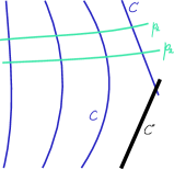
Figure 6. A curve $C$ sprouts off a tail $C^{\prime\prime}$.

We denote by

$$\pi:\mathbf{C}\to B$$

the corresponding family of $2$-pointed rational curves. The dualizing sheaves of the fibers are obtained by restricting

$$\mathscr{K}_{\mathbf{C}}\otimes\pi^{*}\mathscr{K}_{B}^{-1}\cong\mathscr{O}_{\mathbf{C}}(-p_{1}-p_{2}+C^{\prime\prime})$$

to the fibers, where $p_{i}$ denote the sections of $\pi$ given by marked points and $C^{\prime\prime}\subset\mathbf{C}$ is the exceptional divisor. We have

$$\mathscr{O}_{\mathbf{C}}(-p_{1}-p_{2})-\mathscr{O}_{\mathbf{C}}(-p_{1}-p_{2}+C^{\prime\prime})=-\mathscr{O}_{C^{\prime\prime}}(-1)$$

and

$$\pi_{*}\left(V\otimes\mathscr{O}_{C^{\prime\prime}}(-1)\right)=\left(\deg V\big{|}_{C^{\prime\prime}}\right)\cdot\mathscr{O}_{b}$$

by Riemann-Roch. This equals the degree of the bundle $\det\pi_{*}\left(V\otimes\mathscr{O}_{C^{\prime\prime}}(-1)\right)$ on $B$, and hence minus the multiplicity of the corresponding component. ∎

Exercise 203.

What will happen in the above computation if we blow up one the points $p_{1}$ or $p_{2}$ ?

While $\det\mathscr{T}^{1/2}$ may be a square in $\operatorname{Pic}(X)$ which will make $\det\Delta$ also a square by Lemma 202, there is nothing selfdual about the class $\Delta$ which would allow the rigidity arguments to go through. A further modification of the enumerative problem is required for that.

6.2. Relative quasimaps in an example

6.2.1.

The evaluation at $p\in C$ in (152) is a rational map

$$\operatorname{ev}_{p}:\mathsf{QM}\dashrightarrow X$$

defined on the open set $\mathsf{QM}_{\textup{nonsing $p$}}$ of quasimaps nonsingular at $p$. Moduli spaces of relative quasimaps is a resolution of this map, that is, they fit into a diagram

(204)

with a proper evaluation map to $X$. Their construction follows an established path in Gromov-Witten theory [Li1, Li2] and, later, DT theory [LiWu].

6.2.2.

The basic idea behind relative quasimaps may be explained in the most basic example of quasimaps to

$$X=\mathbb{C}/\mathbb{C}^{\times}\,.$$

From definitions

$$\mathsf{QM}(C\to\mathbb{C}/\mathbb{C}^{\times})=\{(\mathscr{L},s)\}\,,$$

where $\mathscr{L}$ is a line bundle on $C$ and

$$s:\mathscr{O}_{C}\to\mathscr{L}$$

is a section which is not identically zero. This gives

$$\mathscr{L}=\mathscr{O}(D)$$

where $D=(s)\in S^{d}C$ is the divisor of $s$ and $d=\deg\mathscr{L}$. Thus

$$\mathsf{QM}(C\to\mathbb{C}/\mathbb{C}^{\times})=\bigsqcup_{d\geq 0}S^{d}C\,.$$

6.2.3.

The set $\mathsf{QM}_{\textup{nonsing $p$}}$ is formed by divisors $D$ disjoint from $p\in C$. Relative quasimaps compactify this set by allowing the curve $C$ to break when the support of $D$ approaches $p$. In the language of algebraic geometry this means the following.

Let $D_{t}$ be a flat $1$-parameter family of divisors parametrized by $t\in B\cong\mathbb{C}$, such that

$$p\in D_{0}\,,\quad p\notin D_{t},\quad\textup{for $t$ generic}\,.$$

We may assume that $p=0\in C\cong\mathbb{C}$, in which case

$$D_{t}=\{f(x,t)=0\}$$

with

(205) $$f(0,0)=0\,,\quad f(0,t)\neq 0\,,\quad f(x,0)\neq 0\,.$$

We will now replace the surface $\mathbf{C}=B\times C$ by a blow-up

$$\mathbf{C}^{\diamond}\to\mathbf{C}$$

such that the proper transform of $D_{t}$ is disjoint from the proper transform of $\{x=0\}$ and from the nodes of the exceptional divisor.

6.2.4.

Let

$$f=\sum_{n,m}f_{n,m}x^{n}t^{m}$$

be the (finite) Taylor expansion of $f$ at $(x,t)=0$. Consider the Newton diagram

$$\textup{Newton}(f)=\textup{Conv}\left(\{(n,m),f_{n,m}\neq 0\}\cup\{(\infty,0),(0,\infty)\}\right)$$

of the polynomial $f$, see Figure 7.

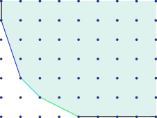
Figure 7. The Newton diagram of a polynomial of the form $x^{5}+\star\,tx^{2}+\star\,t^{2}x+\star\,t^{4}+\dots$, where dots stand for monomials in the shaded area and stars for nonzero numbers. The bounded edges have (minus) slopes $\{\frac{1}{2},1,3\}$.

Let $I$ be the monomial ideal

$$I=(x^{a}t^{b})_{(a,b)\in\textup{Newton}(f)}\,,$$

which by (205) is nontrivial zero-dimensional ideal. As $\mathbf{C}^{\diamond}$, we take the blowup

$$\mathbf{C}^{\diamond}=\operatorname{Bl}_{I}\mathbf{C}$$

of $\mathbf{C}$ in the ideal $I$, that is, the closure of the graph of the map

$$\mathbf{C}\dashrightarrow\mathbb{P}^{\textup{\# of generators}-1}$$

given by the generators of $I$. This is a toric surface whose toric diagram is the Newton diagram. The bounded edges in this diagram correspond to components of the exceptional divisor.

6.2.5.

It is easy to see that, by construction, that the proper transform of $D_{t}$ in $\mathbf{C}^{\diamond}$ satisfies the following properties:

• it is disjoint from the proper transform of $\{x=0\}$,

• it intersects every component of the exceptional divisor,

• it is disjoint from the nodes of the exceptional divisor.

Exercise 206.

Check this.

The only shortcoming of $\mathbf{C}^{\diamond}$ is that fiber $C^{\diamond}$ over $0$ of the induced map

may have multiple components and hence cannot serve as a degeneration of $C$. Indeed, we have the following

Exercise 207.

If $I=(x^{a},t^{b})$ then the multiplicity of the exceptional divisor in $C^{\diamond}$ is $a/\gcd(a,b)$. More generally, if an compact edge in Figure 7 has slope $a/b$ with $\gcd(a,b)=1$ then the corresponding component of the exceptional divisor has multiplicity $a$ in $C^{\diamond}$.

This is remedied by a passing to a degree $m$ branched cover, also known as base change,

where $t=(t^{\prime})^{m}$ and

$$m=\textup{lcm}\,\left\{\frac{a_{i}}{\gcd(a_{i},b_{i})}\right\}_{\textup{slopes $\frac{a_{i}}{b_{i}}$}}\,.$$

The central fiber $C^{\prime}$ in the resulting family

is the curve $C$ with a chain of rational curves (the exceptional divisor) attached, all with multiplicity one.

6.2.6.

We denote by $p^{\prime}\in C^{\prime}$ the intersection of $C^{\prime}$ with the proper transform of $\{x=0\}$ and by $D^{\prime}_{0}$ the intersection of $C^{\prime}$ with the proper transform of $D_{t}$.

Exercise 208.

Show $D^{\prime}_{0}$ is disjoint from $p^{\prime}$ and the nodes of $C^{\prime}$. What is the degree of this divisor on each component of $C^{\prime}$ ?

6.2.7.

In simple English, the blowup $\mathbf{C}^{\diamond}$ and its branched cover $\mathbf{C}^{\prime}$ serve the following purpose.

One can write the solutions $x_{i}(t)$ of the equation $f(x,t)=0$ as Puiseux series

(209) $$x_{i}(t)=c_{i}t^{r_{i}}+o(t^{r_{i}})\,,\quad r_{i}=\frac{b_{i}}{a_{i}}\,,\quad c_{i}\neq 0\,,$$

where $i=1,\dots,\deg_{x}f$. We can assume them ordered in the decreasing order of the rates $r_{i}$ at which they approach $0$ as $t\to 0$.

These rates are the reciprocals of the slopes in Figure 7 and the solutions $x_{i}(t)$ that go to zero at the same rate will end up on the same component of the exceptional divisor, see Figure 8 .

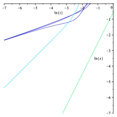
Figure 8. Logarithmic plot of $|x_{i}(t)|$ for a polynomial from Figure 7 as $(x,t)\to(0,0)$. The slopes in this figure are dual, or perpendicular, to the slopes in Figure 7

Suppose, for example, that

$$r_{1}=r_{2}=r_{3}>r_{4}\geq\dots\geq 0$$

Then the component $C^{\prime}_{p^{\prime}}$ of $C^{\prime}$ that contains $p^{\prime}$ will contain $3$ points of $D^{\prime}_{0}$, with coordinates $c_{1},c_{2},c_{3}$, up to proportionality. The up-to-proportionality business appears here because there is no canonical identification $C^{\prime}_{p^{\prime}}\cong\mathbb{P}$ as the only distinguished points of this component are $p^{\prime}$ and the node of $C^{\prime}$.

Put it in a different way, the rescaling

$$t\mapsto\lambda t$$

acts on the leading coefficients in (209) by

$$(c_{1},c_{2},c_{3})\mapsto\lambda^{-r_{1}}(c_{1},c_{2},c_{3}),$$

and so acts nontrivially even on the central fiber.

6.2.8.

This is an important point, and so worth repeating one more time. In the central fiber, we have

1. a chain of rational curves $C^{\prime}$, one end of which is identified with $C$ while the other contains the point $p^{\prime}$,

2. a divisor disjoint from $p^{\prime}$ and the nodes of $C^{\prime}$, and such that its degree on any components other than $C$ is positive,

3. this data is considered up to isomorphism which must be identity on $C$.

A pointed nodal curve $C^{\prime}$ is called stable if it automorphism group is finite. If the automorphism group is reductive, the curve is called semistable. Semistability means some components of $C^{\prime}$ contain only 2 special (that is, marked or nodal) points and the sequence

$$1\to\left(\mathbb{C}^{\times}\right)^{\textup{\# such components}}\to\operatorname{Aut}(C^{\prime})\to\textup{finite group}\to 1$$

is exact.

We extend this terminology to cover cases when one or more components of $C^{\prime}$ are considered as rigid, equivalently, parametrized. In our example, the component $C\subset C^{\prime}$ is rigid. This may be reduced to the usual case by adding enough marked points to rigid components.

There is a stabilization map which collapses nonrigid components with only 2 special points. In the case at hand, $(C,p)$ is the stabilization of $(C^{\prime},p^{\prime})$.

6.2.9.

Instead of constructing $\mathbf{C}^{\diamond}$ and then $\mathbf{C}^{\prime}$ all at once, we could have constructed them in stages as follows. Let $r_{1}$ be the maximal rate at which $x_{i}(t)\to 0$, which means that $1/r_{1}$ is the minimal slope in Figure 7. Write $r_{1}=b_{1}/a_{1}$, $\gcd(a_{1},b_{1})=1$, blow up the ideal $(x^{a_{1}},t^{b_{1}})$, and pass to a branched cover of degree $a_{1}$. This takes care of the points that were approaching $p$ the fastest. Now they all land on the component of $C^{\prime}$ that contains $p^{\prime}$, while all other points of $D_{t}$ approach some point of $C$ as $t\to 0$, including the node of the central fiber.

Obviously, we can deal with points approaching the node inductively, by looking at those that approach the fastest, doing the corresponding blowup, etc.

6.2.10.

Looking at the list in Section 6.2.8, one can make the following important observation. The data of the divisor in central fiber is taken modulo the action of

$$\operatorname{Aut}(C^{\prime},\{C,p\})=\left(\mathbb{C}^{\times}\right)^{\textup{\# of bubbles}}$$

where bubbles refer to components of $C^{\prime}$ other than $C$. The action of this group on divisor can and will have finite stabilizers, so moduli space of objects in Section 6.2.8 is an orbifold.

In fact, the need to go to branched covers precisely correlates with these orbifold singularities.

Exercise 210.

Let $a/b$ with $\gcd(a,b)=1$ be the slope of one of the edges in Figure 7. Show that the restriction of $D^{\prime}_{0}$ to the corresponding component of $C^{\prime}$ is invariant under the group

$$\mu_{a}=\{\zeta\,\big{|}\,\zeta^{a}=1\}\subset\mathbb{C}^{\times}\,.$$

Conversely, if a divisor $D^{\prime}_{0}$ has a nontrivial group of automorphisms, then there exists a family a $1$-parameter family $D_{t}$ producing it for which base change is necessary.

6.3. Stable reduction for relative quasimaps

6.3.1.

We now generalize the discussion of Section 6.2 to quasimaps to a Nakajima variety $X$. A stable quasimap

$$f:C\dasharrow X$$

relative $p\in C$ is defined as a diagram

(211)

in which

1. $\pi$ is the stabilization of a semistable curve $(C^{\prime},p^{\prime})$,

2. $f^{\prime}$ is nonsingular at $p$ and the nodes of $C^{\prime}$,

3. the automorphism group of $f^{\prime}$ is finite.

Figure 9 is a pictorial representation of this data.

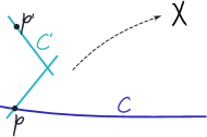
Figure 9. A quasimap relative a point $p\in C$ is a quasimap from a semistable curve $C^{\prime}$ whose stabilization collapses a chain of rational curves to $p$.

Note that nonsingularity at $p$ and the nodes implies $f^{\prime}$ takes the generic point of each component of $C^{\prime}$ to $X$.

Two quasimaps are isomorphic, if they fit into a diagram of the form

where $\phi$ is an isomorphism which preserves the marked point. Since

$$\operatorname{Aut}(C^{\prime},\pi,p)=\left(\mathbb{C}^{\times}\right)^{\textup{\# of new components}}$$

a quasimap has a finite group of automorphism if and only if each component of $C^{\prime}$ is either mapped nonconstantly to $X$ or has at least one singular point.

6.3.2.

A quasimap to $X$ may be composed pointwise with the projection to the affine quotient

$$X_{0}=\mu^{-1}(0)/G=\operatorname{Spec}\left(\textup{$G$-invariants}\right)\,,$$

which has to be constant since $X_{0}$ is affine. This gives a map $\mathsf{QM}(X)\to X_{0}$, and similarly for relative quasimaps.

By a general result of [CKM], the moduli space of both ordinary and relative quasimaps is proper over $X_{0}$. Our goal in this section is to get a feeling for how this works and, in particular, to explain the logic behind the definition of a relative quasimap.

6.3.3.

The key issue here is that of completeness, which means that we should be able to fill in central fibers for maps

$$g:B^{\times}\to\mathsf{QM}(X)_{\textup{relative $p$}}\,,$$

where $B^{\times}=B\setminus\{0\}$ and $B$ is a smooth affine curve with a point $0$, under the assumption that the corresponding map to $X_{0}$ extends to $B$.

6.3.4.

By definition, a map

$$g:B^{\times}\to\mathsf{QM}(f:C\to X)$$

is given by the bundles $\{g^{*}\mathscr{V}_{i}\}$ and the section $f\circ g$ defined on

$$\mathbf{C}^{\times}=C\times B^{\times}\,.$$

The first step to find some extension of the bundles and the section to $\mathbf{C}$. This preliminary extension will satisfy stability on the central fiber, but may fail nonsingularity at $p$.

For simplicity, assume that $C$ is irreducible (otherwise, consider each component of $C$ separately and use nonsingularity of quasimaps at the nodes). The map $g$ yields a rational map in the following diagram

Since $X$ is projective over $X_{0}$, the locus of indeterminacy of $g_{\textup{rational}}$ has codimension $\geq 2$, which means it consists of finitely many points. After shrinking the curve $B$, we may assume all points of indeterminacy lie in the central fiber. This extends the bundles and the section to the generic point of the central fiber.

On a smooth surface $\mathbf{C}$, one can extend a vector bundle from a complement $U$ of a finite set of points by just pushing forward the sheaf of sections under $U\to\mathbf{C}$ (e.g. because such push-forward is reflexive and thus has to be locally free). This procedure automatically extends sections of any associated vector bundle. One usually talks about Hartogs-type theorems when discussing such extensions.

In summary, we have extended the quasimap to the central fiber, except it may be singular at $p$.

6.3.5.

One may consider quasimaps to general quotients of the form

$$X=W/\!\!/G$$

and for properness [CKM] need to assume that $W$ is affine and $G$ is reductive. Both assumptions are essential for the ability to extend a $G$-bundle and the section of the associated $W$-bundle to $\mathbf{C}$.

Indeed, suppose $W$ is not affine. Then it may not be possible to extend a map to $W$ in codimension $2$, as examples $W=\mathbb{C}^{2}\setminus\{0\}$ or $W=\mathbb{P}^{1}$ clearly show. The geometric reason the extension will fail for any $W$ that contains a rational curve is that rational curves in $W$, parametrized or not, will break in families like the curves in Figures 6 or 11. Indeed, take a parametrized curve, precompose with an automorphism, and send the automorphism to infinity. Or, take a double cover of a rational curve and make the branch points collide, etc. Special fibers of the corresponding map $\mathbf{C}\to W$ are thus forced to be reducible.

On the other hand, suppose $G$ is not reductive. After choosing a faithful linear representation, a $G$-bundle may be seen as rank $n$ vector bundle together with its reduction to $G\subset GL(n)$. Such reduction is a section of the associated $GL(n)/G$-bundle and by Matsushima and Onishchik

$$\textup{$G$ is reductive}\,\Leftrightarrow\,\textup{$GL(n)/G$ is affine}\,,$$

see e.g. Section 4.7 in [VinPop]. And so if $G$ were not reductive, there would be $G$ bundles that cannot be extended in codimension 2.

Stable reduction for moduli spaces $\overline{M}_{0,n}(X)$ of stable pointed maps deals with these issues by doing enough blowups, in the course of which the central fiber may become an arbitrary tree of rational curves. As explained in Section 6.1.8, having an arbitrary tree of rational curves is precisely what we are trying to avoid. We need to keep the central fiber a chain of rational curves.

6.3.6.

Also note that for a normal but singular surface $S$ there may be no way to extend a vector bundle on nonsingular locus to a vector bundle on all of $S$.

For instance, the singularities of the surface from Figure 7 are the $2$-dimensional toric singularities, which may be described as follows

(212) $$S =\operatorname{Spec}\mathbb{C}C\,,\quad C=\textup{cone in $\Lambda\cong\mathbb{Z}^{2}$}\,,$$

$$=\mathbb{C}^{2}/\textup{finite abelian subgroup $\Gamma\subset GL(2)$}\,,$$

(213) $$=\mathbb{C}^{2}/\operatorname{diag}(\zeta,\zeta^{a})\,,\quad\zeta^{n}=1,\gcd(n,a)=1\,,$$

where $\mathbb{C}C$ in (212) denotes the semigroup algebra of a cone $C$ and (213) is the explicit description of $\Gamma/\Gamma^{\prime}$ where $\Gamma^{\prime}\subset\Gamma$ is the subgroup generated by complex reflections, i.e. elements with codimension 1 fixed loci. The invariant ring in (213) is of the form $\mathbb{C}C$ where

(214) $$\Lambda=\langle(n,0),(-a,1)\rangle\subset\mathbb{Z}^{2}\,,\quad C=\Lambda\cap\mathbb{Z}_{\geq 0}^{2}$$

and any cone in a rank 2 lattice can be written like that.

Exercise 215.

Check the claim about the singularities and find Weil divisors on these surfaces which are not Cartier divisors, that is, cannot be defined by one equation near the singularity. Conclude that there are line bundles on the nonsingular locus such that their pushforward to all of $S$ is not locally free.

Another way to state the content of the above exercise is the following. Any bundle on $\mathbb{C}^{2}\setminus\{0\}$ is trivial as the restriction of its extension to $\mathbb{C}^{2}$. For the singularity (213), we have

$$S\setminus\{0\}=\left(\mathbb{C}^{2}\setminus\{0\}\right)\big{/}\mu_{n}\,,\quad\mu_{n}=\{\operatorname{diag}(\zeta,\zeta^{a})\}\,.$$

Therefore, a vector bundle on $S\setminus\{0\}$ may be seen as a representation of $\mu_{n}$, and it extends to a vector bundle on the singular surface if and only if this representation is trivial.

6.3.7.

After these remarks, we return to our task of making the quasimap in the central fiber nonsingular at the marked point $p$ by pulling it back under a well-chosen map

$$\mathbf{C}_{1}\to\mathbf{C}\,,$$

which will be a combination of a (weighted) blowup, that is, the blowup of an ideal of the form

$$I=(x^{a},t^{b})\,,\quad\gcd(a,b)=1\,,$$

and a degree $a$ branched cover $t=(t^{\prime})^{a}$, as in Section 6.2. The central fiber

$$C_{1}=E_{1}\cup_{p_{1}}C$$

is the union of the exceptional divisor and the component isomorphic to $C$. We denote by $p_{1}$ the node of the central fiber. The marked point $p\in C_{1}$ lies on $E_{1}$, it is the intersection of $E_{1}$ with the proper transform of $\{x=0\}$, see Figure 10.

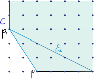
Figure 10. A weighted blowup at slope $3/2$ followed by a base change: we blow up of the ideal $I=(x^{3},t^{2})$ and set $t=(t^{\prime})^{3}$.

Since the vertical map in

is projective, the rational map $g_{1,\textup{rational}}$ is defined at the generic point of $E_{1}$. In English, the restriction $g_{1,\textup{rational}}$ to $E_{1}$ is obtained by taking the lowest degree terms with respect to the grading defined by

$$\deg t^{\prime}=1\,,\quad\deg x=b\,.$$

These lowest degree terms are then a function of the coordinate $x/(t^{\prime})^{b}$ on $E_{1}$.

If the slope $a/b$ is too small, then the map

(216) $$E_{1}\dasharrow X$$

is a constant map which contracts $E_{1}$ to $\lim_{t\to 0}g(0,t)$. (Why does this limit exist ?) Moreover, this map is nonsingular away from the node $p_{1}$. We choose $s$ to be the minimal slope for which this doesn’t happen, that is, the map (216) is either nonconstant or singular at some point of $E_{1}\setminus\{p_{1}\}$. It can be seen that

1. a minimal slope exists,

2. the minimality of the slope implies $g_{1}$ is nonsingular at $p$.

Indeed, if $g_{1}$ were singular at $p$, we could get something nontrivial with a further blowup, which would then have a smaller slope, etc.

Picking a minimal slope means focusing on singularities that approach the marked point the fastest as $t\to 0$, like in Section 6.2.7.

6.3.8.

With the singularities of $g_{1}$ at $E_{1}\setminus\{p_{1}\}$ we deal as in Section 6.3.4 to get a quasimap defined on all of $E_{1}\setminus\{p_{1}\}$.

What remains is the singularity at $p_{1}$. We deal with it inductively, by blowing up this point at the smallest nontrivial slope, and so on. As the degree of the map is consumed at each step, the process will terminate in finitely many steps.

The inductive step in this process is the data of a quasimap on $\mathbf{C}_{n}\setminus\{p_{n}\}$, where $p_{n}$ is the $n$th node of the central fiber. The point $p_{n}$ is a singularity of $\mathbf{C}_{n}$ and, in light of the discussion in Section 6.3.6, we don’t attempt to extend the bundles $\mathscr{V}_{i}$ to $p_{n}$. Eventually, the quasimap will be nonsingular at all nodes and the bundles $\mathscr{V}_{i}$ will be extended by pull-back from $X$.

6.3.9.

Note that unnecessary blowups, like blowing up at too small a slope, or blowing up a node which is already nonsingular, precisely produce quasimaps which are constant and nonsingular along one of the components. Such quasimaps have continuous automorphims and so violate the definition of a stable relative quasimap from Section 6.3.1

6.3.10.

It is also clear that stable reduction, in the form described above, involves no arbitrary choices and its final result is forced on us by the geometry of the quasimap in a punctured neighborhood of $(x,t)=(0,0)$. This can be easily formalized to show that the moduli space of stable relative quasimaps is separated, which means that the limits in $1$-parameter families are unique.

The existence and uniqueness of limits in $1$-parameter families is equivalent, by what is known as the valuative criterion of properness, to $\mathsf{QM}(X)_{\textup{relative $p$}}$ being proper over $X_{0}$. To make this stament precise, we need an actual moduli space for quasimaps, and this is where we turn our attention now.

6.4. Moduli of relative quasimaps

6.4.1.

The construction of the moduli space of stable relative quasimaps may be done, in some sense, by doing stable reduction in reverse, starting with a universal deformation of the curve $C^{\prime}$.

The local model for a deformation of a node is

(217) $$xy=\varepsilon$$

where the precise flavor of the deformation problem depends on how much we rigidify the two coordinate axes. If we rigidify them both completely by adding 2 marked points to each like in Figure 11, then

$$\varepsilon\,\,\propto\,\,\textup{crossratio}(x_{1},x_{2};\frac{\varepsilon}{y_{1}},\frac{\varepsilon}{y_{2}})-1\,,\quad\varepsilon\to 0\,,$$

is the local coordinate on the moduli space $\overline{M}_{0,4}$.

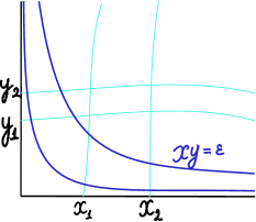
Figure 11. Degeneration of a 4-pointed curve to a stable nodal curve.

If we remove one marked point on one of the axes, then the nodal curve gets a $\mathbb{C}^{\times}$ worth of automorphisms, while all $\varepsilon\neq 0$ curves are become isomorphic. We thus get a moduli stack of the form $\mathbb{C}/\mathbb{C}^{\times}$, where $\varepsilon$ is the coordinate on $\mathbb{C}$. We will indicate this by $\mathbb{C}_{\varepsilon}$ to keep track of the name of the coordinate.

The domain $C^{\prime}$ of a quasimap relative one point $p$ may be exactly this sort of curve, with one rigid component, and the other component with a marked point and $\mathbb{C}^{\times}$ acting by automorphims. A more uniform way to write its universal deformation is to take the trivial family $C\times\mathbb{C}_{\varepsilon}$ and blow up the point $p$ in the central fiber.

6.4.2.

The universal deformation of the domain $C^{\prime}$ of a general relative quasimap may be written analogously. For concreteness, assume $C^{\prime}$ has two nodes. Consider

$$\widetilde{\boldsymbol{C}}=\operatorname{Bl}_{\begin{subarray}{c}\,\,\textup{strict transform}\\ \textup{of }\{\varepsilon_{2}=0\}\times\{p\}\end{subarray}}\operatorname{Bl}_{\{\varepsilon_{1}=0\}\times\{p\}}\mathbb{C}^{2}_{\varepsilon_{1},\varepsilon_{2}}\times C$$

The toric picture of this 3-fold may be seen in Figure 12. An informal, but accurate way to describe this geometry is to compare with an accordion, in which various sections of the bellows open over the divisors $\{\varepsilon_{i}=0\}$.

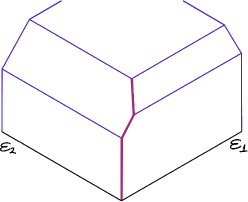
Figure 12. Universal deformation of a curve with two bubbles. The $i$th node remains intact over $\varepsilon_{i}=0$.

The fibers of the map $\boldsymbol{\varepsilon}$ in the diagram

(218)

are deformations of the central fiber $C^{\prime}$ and the group $\left(\mathbb{C}^{\times}\right)^{2}$ acts on the base and on the fibers by isomorphisms. This exhibits the stack of deformations of $C^{\prime}$ as

$$\operatorname{Def}(C^{\prime})=\mathbb{C}^{2}_{\varepsilon_{1},\varepsilon_{2}}\big{/}\left(\mathbb{C}^{\times}\right)^{2}$$

and $\widetilde{\boldsymbol{C}}$ as the universal family over it.

The divisors $\varepsilon_{i}=0$ are the loci where the $i$th node remains intact. The strict transform of $\pi^{-1}(p)$ defines a marked point $p^{\prime}$ in the fibers of $\boldsymbol{\varepsilon}$.

6.4.3.

Assume we already have a construction of ordinary, nonrelative quasimap moduli spaces. Like any good moduli space, quasimaps moduli are defined not just for an individual source curve $C$, but for families of those, that is, for curves over some base scheme.

An example of such family is the universal curve $\widetilde{\boldsymbol{C}}$ over the base $\mathbb{C}^{2}_{\varepsilon_{1},\varepsilon_{2}}$ in (218). The quasimaps from the fibers of $\boldsymbol{\varepsilon}$ fit together in one variety over $\mathbb{C}^{2}_{\varepsilon_{1},\varepsilon_{2}}$ and we can form the quotient

(219) $$\mathsf{QM}_{\begin{subarray}{c}\textup{relative $p$}\\ \textup{$\leq 2$ nodes}\end{subarray}}=\left\{\begin{matrix}[c]\textup{stable quasimaps}\\ \textup{from fibers of $\boldsymbol{\varepsilon}$ to X}\end{matrix}\right\}\bigg{/}\left(\mathbb{C}^{\times}\right)^{2}\,.$$

Here stable means:

• nonsingular at $p^{\prime}$ and at the nodes,

• the $\left(\mathbb{C}^{\times}\right)^{2}$-stabilizer is finite.

The quotient (219) is an open set in the moduli spaces of quasimaps relative $p\in C$. It contains those quasimaps for which the domain breaks at most twice.

6.4.4.

By construction, relative quasimaps come with an evaluation map $\operatorname{ev}_{p}$ at the relative point $p^{\prime}\in C^{\prime}$.

Lemma 220.

The map $\operatorname{ev}_{p}$ is proper for quasimaps of fixed degree.

Proof.

Follows from the properness of the map $\pi$ in the diagram

shown in [CKM] and explained in Section 6.3. ∎

6.4.5.

The deformation theory of the prequotient in (219) is given by the deformation theory (158) of quasimaps from a fixed domain plus the lateral movements along the base $\mathbb{C}^{2}_{\varepsilon_{1},\varepsilon_{2}}$, see [CKM]. Here it is important that the total space $\widetilde{\boldsymbol{C}}$ is smooth and stable quasimaps are nonsingular at the nodes.

Taking the quotient, we get

(221) $$T_{\textup{vir}}\,\mathsf{QM}_{\textup{relative}}=T^{\textup{fixed domain $C^{\prime}$}}_{\textup{vir}}+T\operatorname{Def}(C^{\prime})\,,$$

where the first term is given by (158) and

$$\operatorname{Def}(C^{\prime})\cong\mathbb{C}^{\textup{\# of nodes}}\Big{/}\left(\mathbb{C}^{\times}\right)^{\textup{\# of nodes}}$$

with

$$T\operatorname{Def}(C^{\prime})=\sum_{\textup{nodes $p_{i}\in\mathbb{C}^{\prime}$}}N_{\{\varepsilon_{i}=0\}}-\operatorname{Lie}\operatorname{Aut}(C^{\prime},\pi,p^{\prime})\,.$$

Here $\{\varepsilon_{i}=0\}$ is the Cartier divisor of domains with $i$th node $p_{i}$ intacts.

6.4.6.

If $p_{i}$ is the intersection of components $C_{i-1}$ and $C_{i}$ of $C^{\prime}$ then (217) shows

(222) $$N_{\{\varepsilon_{i}=0\}}=T_{p_{i}}C_{i-1}\otimes T_{p_{i}}C_{i}\,.$$

Since the group $\operatorname{Lie}\operatorname{Aut}(C^{\prime},\pi,p^{\prime})$ acts on these tangent lines, they descend to line bundles on the quotient, typically nontrivial. We will also need the line bundle

(223) $$\psi_{p}=T_{p^{\prime}}^{*}C^{\prime}$$

in what follows.

6.4.7.

After this discussion of the deformation theory for relative quasimaps, we define

(224) $$\widehat{\mathscr{O}}_{\textup{vir}}=\mathscr{O}_{\textup{vir}}\otimes\left(\mathscr{K}^{\textup{fixed domain}}_{\textup{vir}}\,\otimes\,\frac{\det\mathscr{T}^{1/2}\big{|}_{p_{2}}}{\det\mathscr{T}^{1/2}\big{|}_{p_{1}}}\right)^{1/2}\,.$$

The existence of the square root follows from Lemma 198.

6.5. Degeneration formula and the glue operator

6.5.1.

Degeneration formula in Gromov-Witten theory was proven in [Li1, Li2], see also [LiWu] for corresponding constructions in Donaldson-Thomas theory. In K-theoretic GW computations, there is a correction to gluing, discovered in [Giv] and discussed in detail in [Lee]. All these ideas are immediately applicable to quasimaps.

The setting of the degeneration formula is the following. Let a smooth curve $C_{\varepsilon}$ degenerate to a nodal curve

$$C_{0}=C_{0,1}\cup_{p}C_{0,2}\,.$$

like in (217). Degeneration formula counts quasimaps from $C_{\varepsilon}$ in terms of relative quasimaps from $C_{0,1}$ and $C_{0,2}$, where in both cases relative conditions are imposed at the gluing point $p$.

6.5.2.

The basic idea behind the degeneration formula is that as $C_{\varepsilon}$ degenerates, the quasimaps $\mathsf{QM}(C_{\varepsilon}\to X)$ degenerate to quasimaps whose domain is a certain destabilization of $C_{0}$, in which the gluing point $p$ is replaced by a chain of rational curves, like in Figure 13. This is because we require quasimaps to be nonsingular at the nodes and letting the domain curve develop new components is a way to keep the singularities from getting into the node.

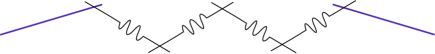
Figure 13. A semistable curve whose stabilization is the nodal curve $C_{0}$. Components with $\mathbb{C}^{\times}$ automorphisms are indicated by springs.

6.5.3.

For a concrete example, take the family (217) and consider quasimaps to $\mathbb{C}/\mathbb{C}^{\times}$, as in Section 6.2. A quasimap to $\mathbb{C}/\mathbb{C}^{\times}$ is a divisor and a family of such is given by a polynomial

$$f(x,y)=0$$

which is not divisible by either $x$ or $y$. The problem could be that $f(0,0)=0$, meaning that a part of the divisor got into the node of $C_{0}$, or that the resulting quasimap $C_{0}\dasharrow X$ is singular at the node.

From Section 6.2.4, we know exactly what to do. We take the toric blowup of the plane corresponding to the Newton diagram of $f$, as in Figure 7. This sends the points which were approaching the origin from different directions to different components of the exceptional divisor.

While the procedure is exactly the same, its interpretation is different: the limiting curve is the exceptional divisor together with both coordinate axes. Those are the two components of $C_{0}$ and the exceptional curves are the new components the domain had to develop so as to keep the singularities away from the nodes.

6.5.4.

This motivates defining $\mathsf{QM}(C_{0}\to X)$ in spirit of Section 6.3.1 as the moduli spaces of quasimaps of the form

(225)

in which

1. the map $\pi$ collapses a chain of rational curves to the node of $C_{0}$,

2. $f^{\prime}$ is nonsingular at the nodes of $C^{\prime}_{0}$,

3. the automorphism group of $f^{\prime}$ is finite.

Here the source of automorphisms is the group

$$\operatorname{Aut}(C^{\prime}_{0},\pi)=\left(\mathbb{C}^{\times}\right)^{\textup{\# of new components}}\,.$$

6.5.5.

Domain curves of the form $C^{\prime}_{0}$, and quasimaps from those curves, are commonly known as accordions, see Figure 14. Indeed, they have two rigid components, and a chain of components rescaled by automorphisms. One may call those nonrigid components bellows, bubbles, etc.

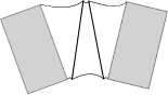
Figure 14. A poetic representation of a semistable curve which stabilizes to a nodal curve.

6.5.6.

The obstruction theory is defined on the total space of the family

$$\epsilon:\mathsf{QM}(C_{\varepsilon}\to X)\to\mathbb{C}$$

and gives a sheaf whose restriction to fibers is the virtual structure sheaf of the fiber. We thus can do K-theoretic counts on any fiber by pulling back the corresponding point class from $\mathbb{C}$. In particular, the counts for $\varepsilon=1$ and $\varepsilon=0$ are equal.

This is very close to what we wanted, in that it gives the counts of quasimaps from the generic fiber in terms of quasimaps from the special fiber. What remains is to separate the quasimaps from the special fibers into contributions of the two components. This is done as follows.

6.5.7.

Suppose the curve $C_{0}^{\prime}$ has $n$ nodes and let $\varepsilon_{1},\dots,\varepsilon_{n}$ be smoothing parameters for each of these nodes. In the corresponding chart on quasimap moduli, we have the equality of divisors

$$(\varepsilon)=(\varepsilon_{1}\varepsilon_{2}\cdots\varepsilon_{n})\,.$$

Exercise 226.

See how this works in the concrete case of Section 6.5.3.

Geometrically, $\varepsilon_{1}\varepsilon_{2}\cdots\varepsilon_{n}=0$ is the union of coordinate hyperplanes, and we have an inclusion-exclusion formula for the K-theory class of this union, namely

(227) $$\mathscr{O}_{\varepsilon_{1}\varepsilon_{2}\cdots\varepsilon_{n}=0}=\sum_{\varnothing\neq S\subset\{1,\dots,n\}}(-1)^{|S|-1}\mathscr{O}_{\bigcap_{i\in S}\{\varepsilon_{i}=0\}}\,,$$

where the summation is over all nonempty subsets $S$ of hyperplanes, that is, to a nonempty subset of nodes of $C_{0}^{\prime}$.

Exercise 228.

Prove (227).

Geometrically, the term in (227) that corresponds to a given collection of $k=|S|$ nodes computes the contribution of quasimaps whose domain has those $k$ nodes intact. The sum over all $S$ such that $|S|=k$ may be interpreted as the count of quasimaps from domains with $k$ marked nodes.

These quasimaps counts can be glued out of $k+1$ pieces as follows.

6.5.8.

Let $C$ be a curve with a marked node obtained by gluing two curves at marked points

$$C=(C_{1},p_{1})\sqcup(C_{2},p_{2})\Big{/}p_{1}\sim p_{2}\,.$$

A quasimap from $C$ is a quasimap from each component plus the requirement that it has takes well-defined and equal values at $p_{1}$ and $p_{2}$. In other words, we have a product over the evaluation maps to $X$

(229) $$\mathsf{QM}(C\to X)_{\textup{marked node}}=\\ =\mathsf{QM}(C_{1}\to X)_{\textup{relative $p_{1}$}}\times_{X}\mathsf{QM}(C_{2}\to X)_{\textup{relative $p_{2}$}}$$

and an inspection of the obstruction theory shows

(230) $$\chi(\mathsf{QM}(C\to X)_{\textup{marked node}},\mathscr{O}_{\textup{vir}})=\chi\left(X,\operatorname{ev}_{p_{1},*}(\mathscr{O}_{\textup{vir}})\otimes\operatorname{ev}_{p_{2},*}(\mathscr{O}_{\textup{vir}})\right)\,.$$

The corresponding formula for the symmetrized virtual class $\widehat{\mathscr{O}}_{\textup{vir}}$ from (201) is the following.

Note that fibers of the polarization at marked points enter asymmetrically in the formula (201). This is very convenient when dealing with chains of rational curves. If the choices are made consistently, the polarization terms for two marked points glued at a node cancel. We assume this is the case, and so we are left with the contribution of $\mathscr{K}_{X}$ to $\mathscr{K}_{\textup{vir}}$. We define

(231) $$(\mathscr{F},\mathscr{G})_{X}=\chi(X,\mathscr{F}\otimes\mathscr{G}\otimes\mathscr{K}_{X}^{-1/2})\,.$$

Then

(232) $$\chi(\mathsf{QM}(C\to X)_{\textup{marked node}},\widehat{\mathscr{O}}_{\textup{vir}})=\chi\left(\operatorname{ev}_{p_{1},*}(\widehat{\mathscr{O}}_{\textup{vir}}),\operatorname{ev}_{p_{2},*}(\widehat{\mathscr{O}}_{\textup{vir}})\right)_{X}\,.$$

6.5.9.

There is a parallel gluing formula for curves with $k$ marked nodes, except it involves a novel kind of quasimaps whose domains are pure accordion bellows, without rigid components.

We define $\mathsf{QM}^{\text{\normalsize$\sim$}}_{\textup{relative $p_{1},p_{2}$}}$ as the moduli space of stable quasimaps with whose domain $C$ is a chain of rational curves joining $p_{1}$ and $p_{2}$. By definition, stability means nonsingularity at $p_{1}$, $p_{2}$, and the nodes, together with being stabilized by a finite subgroup in

$$\operatorname{Aut}(C,p_{1},p_{2})=(\mathbb{C}^{\times})^{\textup{\# of components}}\,.$$

Since a constant quasimap from a nonrigid two-pointed curve is unstable, we make a separate definition

$$\mathsf{QM}^{\text{\normalsize$\sim$}}_{\textup{relative $p_{1},p_{2}$,degree 0}}=\mathsf{QM}(\textup{point}\to X)=X\,.$$

In other words, when bellows don’t open, we define $C$ to be a point.

We define

(233) $$\mathbf{G} =(\operatorname{ev}_{p_{1}}\times\operatorname{ev}_{p_{2}})_{*}\,\widehat{\mathscr{O}}_{\textup{vir}}\,z^{\deg f}$$

$$=\operatorname{diag}\mathscr{K}^{1/2}_{X}+O(z)\,,$$

where $O(z)$ stands for the contribution of nontrivial quasimaps. Clearly, the counts of curves with $k$ marked nodes may be expressed as a certain multiple convolution of relative curve counts like in (232) with this tensor. It is convenient to have an operator notation to express this convolution.

6.5.10.

We have a natural convolution action

$$K(X\times X)\otimes_{K(\textup{pt})}K(X)\to K(X)_{\textup{localized}}\,.$$

given by

$$(\mathscr{E},\mathscr{F})\mapsto p_{1,*}\left(\mathscr{E}\otimes p_{2}^{*}\mathscr{F}\right)\,.$$

For decomposable classes

$$K(X)^{\otimes 2}\subset K(X\times X)$$

this action corresponds to the bilinear form $(\mathscr{E},\mathscr{F})\mapsto\chi(\mathscr{E}\otimes\mathscr{F})$.

In our situation, the form is twisted by $\mathscr{K}^{-1/2}_{X}$ (which is a pure equivariant weight, to be sure) as in (231), and we similarly twist the convolution action to

(234) $$(\mathscr{E},\mathscr{F})\mapsto p_{1,*}\left(\mathscr{E}\otimes p_{2}^{*}\mathscr{F}\otimes\mathscr{K}^{-1/2}_{X}\right)\,.$$

With this convention (we will see in a moment that localization is not required)

(235) $$\mathbf{G}=1+O(z)\in\operatorname{End}K(X)[[z]]$$

as an operator on $K(X)$. We call it the gluing operator. From (235) we see it is invertible in $\operatorname{End}K(X)[[z]]$.

Exercise 236.

Generalizing (232) prove

(237) $$\chi(\mathsf{QM}(C\to X)_{\textup{$k$ marked nodes}},\widehat{\mathscr{O}}_{\textup{vir}}\,z^{\deg f})=\\ =\chi\left((\mathbf{G}-1)^{k-1}\operatorname{ev}_{p_{1},*}(\widehat{\mathscr{O}}_{\textup{vir}}\,z^{\deg f}),\operatorname{ev}_{p_{2},*}(\widehat{\mathscr{O}}_{\textup{vir}}\,z^{\deg f})\right)_{X}\,.$$

6.5.11.

From formulas (227) and (237) we deduce the following

Proposition 238 ([Giv, Lee]).

We have

(239) $$\chi(\mathsf{QM}(C_{0}\to X),\widehat{\mathscr{O}}_{\textup{vir}}\,z^{\deg f})=\\ =\left(\mathbf{G}^{-1}\operatorname{ev}_{1,*}(\widehat{\mathscr{O}}_{\textup{vir}}\,z^{\deg f}),\operatorname{ev}_{2,*}(\widehat{\mathscr{O}}_{\textup{vir}}\,z^{\deg f})\right)_{X}\,,$$

where

$$\operatorname{ev}_{i}:\mathsf{QM}(C_{0,i}\to X)_{\textup{relative gluing point}}\to X$$

are the evaluation maps.

Proof.

Follows from

$$\sum_{k\geq 1}(-1)^{k-1}(\mathbf{G}-1)^{k-1}=\mathbf{G}^{-1}\,.$$

∎

6.5.12.

We also have the following

Proposition 240.

The glue operator $\mathbf{G}$ acts in nonlocalized $K$-theory of $X$.

Proof.

Recall that $X_{0}$ denotes the affinization of the Nakajima variety $X$. Since every quasimap is contracted by the map to $X_{0}$, the evaluation map in (233) is a proper map to

(241) $$\textup{Steinberg variety}:=X\times_{X_{0}}X\subset X\times X\,.$$

Since the map $X\to X_{0}$ is proper, any class supported on the Steinberg variety acts in nonlocalized K-theory. ∎

7. Nuts and bolts

7.1. The Tube

7.1.1.

We define

(242) $$\mathsf{Tube}=\operatorname{ev}_{*}\left(\mathsf{QM}_{\textup{relative $p_{1},p_{2}$}}\,,\widehat{\mathscr{O}}_{\textup{vir}}\,z^{\deg f}\right)\in K(X)^{\otimes 2}\otimes\mathbb{Q}[[z]]\,,$$

and make it an operator acting from the second copy of $K(X)$ to the first using the bilinear form (231) or, more precisely, the formula (234).

Just like in the case of the gluing matrix $\mathbf{G}$ considered in Proposition 240, the operator $\mathsf{Tube}$ acts in nonlocalized K-theory of $X$.

7.1.2.

Theorem 243.

We have

(244) $$\mathsf{Tube}=\mathbf{G}$$

It will be instructive to go through two very different proofs of this statement. The first one is very short.

First proof.

The degeneration formula (239) gives

$$\mathsf{Tube}=\mathsf{Tube}\,\mathbf{G}^{-1}\mathsf{Tube}\,.$$

Therefore, the operator $P=\mathsf{Tube}\,\mathbf{G}^{-1}$ satisfies

$$P^{2}=P\,.$$

Since $P=1+O(z)$, this projector is invertible, whence $P=1$ . ∎

7.1.3.

Let $\mathbb{C}^{\times}$ act on $C\cong\mathbb{P}^{1}$ with fixed points $p_{1}$ and $p_{2}$. Denote

$$q=\textup{weight of $T_{p_{1}}C$}\,.$$

We will denote this group $\mathbb{C}^{\times}_{q}$ to distinguish it from other tori present.

For our second proof of Theorem 243, we will use $\mathbb{C}^{\times}_{q}$-equivariant localization. For this, we need a description of the $\mathbb{C}^{\times}_{q}$-fixed quasimaps.

7.1.4.

Let $f$ be a $\mathbb{C}^{\times}_{q}$-fixed quasimap. By stability, its singularities in $C\setminus\{p_{1},p_{2}\}$ form a set which is

$$\textup{finite and $\mathbb{C}^{\times}_{q}$-invariant}\Rightarrow\textup{empty}\,.$$

For maps relative $\{p_{1},p_{2}\}$, this means that all singularities appear in the accordions and $f\big{|}_{C}$ is constant map to a point in $X$. In particular, all bundles $\mathscr{V}_{i}\big{|}_{C}$ are trivial.

In general, for the $\mathbb{C}^{\times}_{q}$-fixed quasimaps there is a unique $\mathbb{C}^{\times}_{q}$-equivariant structure on the bundles $\mathscr{V}_{i}$ compatible with the quiver maps and the trivial equivariant structure on the bundles $\mathscr{W}_{i}$ and $\mathscr{Q}_{ij}$. In our case, $\mathbb{C}^{\times}_{q}$ acts trivially on the trivial bundles $\mathscr{V}_{i}\big{|}_{C}$.

7.1.5.

We conclude the only part of the deformation theory on which $\mathbb{C}^{\times}_{q}$ acts are the normal direction to the fixed locus. These correspond to the smoothing of the nodes at $p_{i}\in C$, when the nodes are present. For example, the contribution of the accordions at $p_{1}$ is

(245) $$\operatorname{ev}_{*}\left(\mathsf{QM}^{\text{\normalsize$\sim$}}_{\textup{relative $p^{\prime}_{1},p_{1}$}}\,,z^{\deg}\,\widehat{\mathscr{O}}_{\textup{vir}}\,\frac{1}{1-q^{-1}\psi_{p_{1}}}\right)\in K(X)^{\otimes 2}\otimes\mathbb{Q}[[q^{-1}]][[z]]$$

because by (222)

$$N_{\textup{$\exists$ node at $p_{1}\in C^{\prime}$}}=\psi^{\vee}_{p_{1}}\otimes q\,.$$

7.1.6.

Each $z$-coefficient in (245) is a rational function of $q$ by the following

Lemma 246.

Let $Y$ be a projective scheme and $\mathscr{L}$ an orbifold line bundle on $Y$. Then for any coherent sheaf $\mathscr{F}$ the series

$$\chi(q)=\chi\left(Y,\frac{\mathscr{F}}{1-q^{-1}\mathscr{L}}\right)=\sum_{k\geq 0}q^{-k}\chi(Y,\mathscr{F}\otimes\mathscr{L}^{k})$$

is a rational function of $q$ such that

$$\chi(0)=0\,,\quad\chi(\infty)=\chi(Y,\mathscr{F})\,.$$

Proof.

By orbifold Riemann-Roch (or by the theory of Hilbert polynomial), we have

$$\chi(Y,\mathscr{F}\otimes\mathscr{L}^{k})=\textup{polynomial in $\{k,\zeta_{i}^{k}\}$}$$

for some roots of unity $\zeta_{i}$ (and, in equivariant situation, also in $w_{i}^{k}$, where $w_{i}$’s are certain weights of $\operatorname{Aut}(X)$). For any function of the form $f(k)=k^{m}t^{k}$ we have

$$\sum_{k\geq 0}f(k)\,q^{-k}=\left(q\frac{d}{dq}\right)^{m}\frac{1}{1-t/q}\to\begin{cases}0\,,&q\to 0\\ f(0)\,,&q\to\infty\,,\end{cases}$$

the lemma follows. ∎

7.1.7.

Second proof of Theorem 243.

Since the pushforward in (242) is proper, the result is a Laurent polynomial in $q$. From Lemma 246 we conclude that

$$\textup{operator defined by \eqref{accord1}}\to\begin{cases}1\,,&q\to 0\\ \mathbf{G}\,,&q\to\infty\,,\end{cases}$$

where $1$ is the contributions of the degree $0$, that is, empty accordions.

For the accordions at $p_{2}$, the analysis is the same with $q$ replaced by $q^{-1}$, therefore

$$\mathsf{Tube}\to\mathbf{G}\,,\quad q\to\{0,\infty\}$$

and the theorem follows. ∎

7.1.8.

It is convenient to use the following shorthand script for the kind of computations that we will be doing in this section. We compute with quasimaps from chains of rational curves, with two or one marked points at the ends, and the corresponding K-theoretic counts are naturally interpreted as operators or vectors in $K(X)[[z]]$, compare with the discussion in Section 3.5.9. To denote these operators, and the order in which they compose, we can simply draw the quasimap domains, with the marked points, nodes, etc.

In our chain of rational curves, we can have two kinds of components: the rigid (or parametrized) ones, and those with only two special points and $\mathbb{C}^{\times}$ worth of automorphisms. We call the latter elastic and denote

a ridig component

an elastic component .

We can have several kinds of marked points, depending on the constraints we put on quasimaps at that marked point. The basic marked points, with no constraints, is denoted by

      a marked point .

If we require the quasimap to be nonsingular at a marked point, we draw an open circle:

      a nonsingular point .

Quasimaps relative to a point will be denoted

      a relative point .

Also, nodes count among the special points

      a node .

7.1.9.

For example, in this shorthand, the degeneration and gluing formulas say

(247) $$\includegraphics[scale={0.5}]{straight_line.eps}\quad=\\ \includegraphics[scale={0.6}]{node.eps}=\quad\\ \raisebox{-4.0pt}{\includegraphics[scale={0.5}]{relative_point_right.eps}}\,\,\mathbf{G}^{-1}\,\raisebox{-4.0pt}{\includegraphics[scale={0.5}]{relative_point.eps}}$$

where

$$\mathbf{G}=\raisebox{-5.0pt}{\includegraphics[scale={0.5}]{glue.eps}}$$

is the gluing matrix.

Similarly, we have

$$\mathsf{Tube}=\raisebox{-5.0pt}{\includegraphics[scale={0.5}]{tube.eps}}$$

and the argument in Section 7.1.2 can be drawn as follows

(248) $$\includegraphics[scale={0.5}]{tube.eps}\quad=\\ \includegraphics[scale={0.6}]{tube_node.eps}=\quad\\ \raisebox{-4.0pt}{\includegraphics[scale={0.5}]{tube.eps}}\,\,\mathbf{G}^{-1}\,\raisebox{-4.0pt}{\includegraphics[scale={0.5}]{tube.eps}}\,.$$

7.2. The Vertex

7.2.1.

As in (204), consider the open set

$$\mathsf{QM}_{\textup{nonsing $p_{2}$}}\subset\mathsf{QM}$$

of quasimaps nonsingular at $p_{2}$ and define

(249) $$\mathsf{Vertex}=\operatorname{ev}_{p_{2},*}\left(\mathsf{QM}_{\textup{nonsing $p_{2}$}}\,,\widehat{\mathscr{O}}_{\textup{vir}}\,z^{\deg f}\right)\in K(X)_{\textup{localized}}\otimes\mathbb{Q}[[z]]\,.$$

This object may also be called K-theoretic Givental’s $I$-function.

While the pushforward in (249) is not proper, we will see the fixed loci of the $\mathbb{C}^{\times}_{q}$-action are proper, so the pushforward is defined in localized K-theory.

7.2.2.

More generally, let

$$\lambda\in K_{G}(\textup{pt})$$

be a virtual representation of the group $G$ in (145). It is a tensor polynomial in the defining representations $V_{i}$, something like $\lambda=V_{1}\otimes V_{2}-\Lambda^{3}V_{2}$.

The polynomial $\lambda$ may be evaluated on the fibers $\mathscr{V}_{i}\big{|}_{p_{1}}$ over the point $p_{1}$. We can define the vertex with descendents by

(250) $$\left\langle\lambda\right|=\operatorname{ev}_{p_{2},*}\left(\mathsf{QM}_{\textup{nonsing $p_{2}$}}\,,\widehat{\mathscr{O}}_{\textup{vir}}\,z^{\deg f}\,\lambda\left(\mathscr{V}\big{|}_{p_{1}}\right)\right)\,.$$

In particular

$$\left\langle 1\right|=\mathsf{Vertex}\,.$$

Also note that by (154)

(251) $$\left\langle\det V_{i}\otimes\lambda\right|=\det V_{i}\otimes\left\langle\lambda\right|\Big{|}_{z_{i}\mapsto qz_{i}}\,,$$

which is essential point behind the difference equations for the vertex that will be discussed at length below.

7.2.3.

Let $f$ be a $\mathbb{C}^{\times}_{q}$-fixed quasimap in $\mathsf{QM}_{\textup{nonsing $p_{2}$}}$. As in Section 7.1.4, this implies that $f\big{|}_{C\setminus\{p_{1}\}}$ is a map to a point $x\in X$. We can identify the trivial bundles $\mathscr{V}_{i}\big{|}_{C\setminus\{p_{1}\}}$ and quiver maps between them with the quiver data for the point $x\in X$.

Define

$$\mathbb{V}_{i}=\bigoplus_{k\in\mathbb{Z}}\mathbb{V}_{i}[k]=H^{0}(\mathscr{V}_{i}\big{|}_{C\setminus\{p_{2}\}})\,,$$

where $\mathbb{V}_{i}[k]$ is the subspace of weight $k$ with respect to $\mathbb{C}^{\times}_{q}$. By invariance, all quiver maps preserve this weight decomposition. We define the framing spaces $\mathbb{W}[k]$ in the same way and obtain

(252) $$\mathbb{W}_{i}[k]=\begin{cases}W_{i}\,,&k\leq 0\,,\\ 0\,,&k>0\,,\\ \end{cases}$$

because the bundles $\mathscr{W}_{i}$ are trivial.

Multiplication by the coordinate induces an embedding

$$\mathbb{V}_{i}[k]\hookrightarrow\mathbb{V}_{i}[k-1]\hookrightarrow\dots\hookrightarrow\mathbb{V}_{i}[-\infty]=V_{i}\,,$$

compatible with quiver maps, where $V_{i}$ is the quiver data for $x$. Thus

(253) $$\left(\mathsf{QM}_{\textup{nonsing $p_{2}$}}\right)^{\mathbb{C}^{\times}_{q}}=\left\{\begin{matrix}\textup{flags of quiver subrepresentations}\\ \textup{satisfying \eqref{bbW}}\end{matrix}\right\}\,.$$

In particular, the space of flags (253) inherits a perfect obstruction theory from the ambient space of quasimaps .

7.2.4.

Recall that $\theta$ denotes the stability parameter for the quiver.

Lemma 254.

We have

$$\mathbb{V}[k] =0\quad \theta\cdot\dim\mathbb{V}[k] >0\,, \quad k >0\,,$$ or

(255) $$\mathbb{V}[k] =V\quad \theta\cdot\dim\mathbb{V}[k] >\theta\cdot\dim V\,, \quad k \leq 0\,.$$ or

Proof.

It is convenient to use the reformulation of quiver stability given by Crawley-Boevey, see in particular Section 3.2 in [GinzNak]. In this reformulation, one trades the framing spaces for an extra vertex $\{\infty\}$, with

$$\dim V_{\infty}=1$$

and $\dim W_{i}$ arrows to every other vertex $i$.

The stability parameter is extended by

$$\theta_{\infty}=-\theta\cdot\dim V$$

and the stability condition reads

$$(\theta,\theta_{\infty})\cdot(\dim V^{\prime},\dim V^{\prime}_{\infty})>0$$

for every nontrivial subrepresentation $V^{\prime}\subset V$. Since

(256) $$\dim\mathbb{V}_{\infty}[k]=\begin{cases}1\,,&k\leq 0\,,\\ 0\,,&k>0\,,\\ \end{cases}$$

the lemma follows. ∎

7.2.5.

We have

(257) $$\deg f=\left(\deg\mathscr{V}_{i}\right)=\sum_{k\in\mathbb{Z}}\Big{(}\dim\mathbb{V}_{i}[k]-\delta_{\{k\leq 0\}}\,\dim V_{i}\Big{)}\,.$$

Let

$$C_{\textup{ample}}\subset H^{2}(X,\mathbb{R})$$

be the closed ample cone of $X$. It is the closure of a neighborhood of $\mathbb{R}_{>0}\,\theta$ formed by those $\theta^{\prime}$ which give an isomorphic GIT quotient. By Lemma 254,

$$\Big{(}\dim\mathbb{V}_{i}[k]-\delta_{\{k\leq 0\}}\,\dim V_{i}\Big{)}\in C_{\textup{ample}}^{\vee}\,,\quad\forall k\,.$$

This bounds the dimensions of $\mathbb{V}_{i}[k]$ for fixed degree and gives the following

Corollary 258.

The map

$$\operatorname{ev}_{p_{2}}:\left(\mathsf{QM}_{\textup{nonsing $p_{2}$}}\right)^{\mathbb{C}^{\times}_{q}}\to X$$

is proper for quasimaps of fixed degree. The moduli space is empty for degrees outside $C_{\textup{ample}}^{\vee}$.

7.2.6.

In many instances, one can use equivariant localization with respect to an additional torus may be used to compute the vertex. If a torus $\mathsf{T}$ acts on $X$ then $\mathbb{C}^{\times}_{q}\times\mathsf{T}$ fixed quasimaps are given in terms of flags $\mathbb{V}_{i}[k]$ that are additionally graded by the weights of $\mathsf{T}$.

The quiver maps are required to be $\mathsf{T}$-equivariant, in particular, to shift the weight if the $\mathsf{T}$-action on the corresponding arrow is nontrivial. Similarly, the framing spaces $\mathbb{W}_{i}$ acquire an additional grading.

The characters of all these spaces are uniquely reconstructed by

(259) $$\mathbb{V}[k]\cong\left(\mathscr{V}\big{|}_{p_{1}}\right)_{\textup{$q$-weight $\geq k$}}$$

from the character of $\mathbb{C}^{\times}_{q}\times\mathsf{T}$ on the fiber of $\mathscr{V}$ at $p_{1}$. Similarly, the character of the deformation theory (158) is directly computable from the character of $\mathscr{V}\big{|}_{p_{1}}$ by localization.

Exercise 260.

Spell out the localization formula for the vertex for $X=T^{*}\operatorname{Gr}(k,n)$.

Exercise 261.

Write a code that computes the vertex function for the Hilbert scheme of points in $\mathbb{C}^{2}$.

7.2.7.

While localization, especially in the case of isolated fixed points, gives a certain computational handle on the vertex, a much more powerful way to compute to compute the vertex is to identify a $q$-difference equation that it satisfies. This identification will require a certain development of the theory.

7.3. The index limit

7.3.1.

Let a torus $\mathsf{A}$ act on $X$ preserving the symplectic form. A dramatic simplification occurs in the localization formulas if we let the equivariant variable $a\in\mathsf{A}$ go to one of the infinities of the torus.

Very abstractly, suppose

$$X=T^{*}M/\!\!/\!\!/\!\!/G$$

and let a torus $\mathsf{A}$ act on $M$ commuting with $G$. For every component $F\subset X^{\mathsf{A}}$ we can assume that $\mathsf{A}$ acts so that

$$F=T^{*}\!\!\left(M^{\mathsf{A}}\right)/\!\!/\!\!/\!\!/G\,.$$

Because we consider quasimaps from a fixed domain, on which $\mathsf{A}$ is not allowed to act, we conclude that

$$\iota_{\mathsf{QM}}:\mathsf{QM}(F)\to\mathsf{QM}(X)^{\mathsf{A}}$$

is an inclusion of a component. Its virtual normal bundle is

(262) $$N_{\textup{vir}}={H}^{\raisebox{1.42262pt}{$\scriptscriptstyle\bullet$}}\left(\mathscr{T}^{1/2}_{\textup{moving}}\oplus\hbar^{-1}\left(\mathscr{T}^{1/2}_{\textup{moving}}\right)^{\vee}\right)\,,$$

where the subscript refers to the $\mathsf{A}$-moving part of the restriction of the polarization to $X^{\mathsf{A}}$.

As in Lemma 198, we conclude

(263) $$N_{\textup{vir}}=\sum_{i=1}^{2}\mathscr{T}^{1/2}_{\textup{moving}}\big{|}_{p_{i}}+H-\hbar^{-1}H^{\vee}\,,\quad H={H}^{\raisebox{1.42262pt}{$\scriptscriptstyle\bullet$}}\left(\mathscr{T}^{1/2}_{\textup{moving}}\otimes\mathscr{K}_{C}\right)\,.$$

7.3.2.

Consider a balanced virtual $\mathsf{A}$-module $H-\hbar^{-1}H^{\vee}$. Its contribution to $\mathscr{O}_{\textup{vir}}\otimes\mathscr{K}_{\textup{vir}}^{1/2}$ is

$$\widehat{\mathsf{a}}\left(H-\hbar^{-1}H^{\vee}\right)\to(-\hbar^{-1/2})^{\operatorname{rk}H_{+}-\operatorname{rk}H_{-}}\,,\quad a\to 0\,,$$

where

$$H=H_{+}\oplus H_{-}$$

is the decomposition of $H$ into attracting and repelling subspaces as $a\to 0$. By Riemann-Roch,

$$\operatorname{rk}H_{+}=\deg\mathscr{T}^{1/2}_{>0}-\operatorname{rk}\mathscr{T}^{1/2}_{>0}\,,$$

and similarly for $H_{-}$.

Taking into account the asymmetry between marked points in (201), the contribution of the first term in (263) to $\widehat{\mathscr{O}}_{\textup{vir}}$ equals

$$\left(\frac{\det\mathscr{T}^{1/2}_{\textup{moving},p_{2}}}{\det\mathscr{T}^{1/2}_{\textup{moving},p_{1}}}\right)^{1/2}\bigotimes_{i=1}^{2}{\widehat{\mathsf{S}}}^{\raisebox{1.42262pt}{$\scriptscriptstyle\bullet$}}\left(\mathscr{T}^{1/2}_{\textup{moving}}\big{|}_{p_{i}}\right)^{\vee}\,,$$

where the symmetric algebra with a hat was defined in (19). Note that this has a nontrivial $q$-weight. Its analysis leads to $q$-dependence in the following

Lemma 264.

As $a\to 0$,

(265) $$\mathsf{Vertex}_{X}\to\hbar^{\frac{\operatorname{codim}}{4}}\,(-\hbar^{-1/2})^{\deg\mathscr{N}_{>0}}q^{-\deg\mathscr{T}^{1/2}_{<0}}\,Vertex_{X^{\mathsf{A}}}\,,$$

where

$$\mathscr{N}_{>0}=\mathscr{T}^{1/2}_{>0}+\hbar^{-1}\left(\mathscr{T}^{1/2}_{<0}\right)^{\vee}$$

is the attracting part of the normal bundle to $X^{\mathsf{A}}$.

For the full vertex, that is, the sum over all degrees with weight $z^{\deg}$, the relationship (265) means a shift of the argument $z$ by a monomial in $(-\hbar^{-1/2})$ and $q$.

7.4. Cap and capping

7.4.1.

In parallel to (250), we define the capped descendents

(266) $$\left\langle\lambda\right\|=\operatorname{ev}_{p_{2},*}\left(\mathsf{QM}_{\textup{relative $p_{2}$}}\,,\widehat{\mathscr{O}}_{\textup{vir}}\,z^{\deg f}\,\lambda\left(\mathscr{V}\big{|}_{p_{1}}\right)\right)\in K(X)\otimes\mathbb{Q}[[z]]\,.$$

Note that in contrast to the vertex, this is a proper pushforward, hence an element of nonlocalized K-theory. Precisely because it is a element of nonlocalized K-theory, it is in many ways a simpler object than the vertex.

By construction,

(267) $$\left\langle\lambda\right\|=\lambda(V)\,\mathscr{K}_{X}^{1/2}+O(z)$$

where $O(z)$ stands for contribution of nonconstant maps. We will see that for many insertions $\lambda$ the cap (266) is purely classical, that is, the $O(z)$ term in (267) vanishes.

7.4.2.

In the shorthand of Section 7.1.8, we have

the vertex ,

the cap .

As in Section 7.1.5, localization gives

(268) $$\raisebox{-2.0pt}{\includegraphics[scale={0.33}]{cap.eps}}\quad=\quad\raisebox{-2.0pt}{\includegraphics[scale={0.33}]{vertex.eps}}\,\,\raisebox{-9.0pt}{\includegraphics[scale={0.4}]{capping.eps}}\,,$$

where the subscript $\psi$ in the

(269) $$\left|\textup{capping operator}\right|=\,\,\raisebox{-11.0pt}{\includegraphics[scale={0.5}]{capping.eps}}$$

indicates the insertion of the cotangent line in the accordion count as in (245).

7.4.3.

One can view (268) as a linear equation for the vertex. The matrix (269) of this linear equation is invertible and, in fact, will be identified with the fundamental solution of a certain $q$-difference equation in what follows.

The constant term, or the left-hand side, of this linear equation will be computed using the vanishing of quantum terms in (267) once the dimensions of the framing spaces are sufficiently large and the polarization is chosen accordingly.

7.5. Large framing vanishing

7.5.1.

Our proof of vanishing of the quantum terms in (267) will follow the logic of the second proof of Theorem 243, namely, it will be based on the analysis of the integrand in the $q\to\{0,\infty\}$ limits. In contrast to the situation considered in Section 7.1.7 , the group $\mathbb{C}^{\times}_{q}$ may now act nontrivially in the fiber $\mathscr{V}\big{|}_{p_{1}}$ over its fixed point $p_{1}$ and the weights of this action have to be analyzed.

Concretely, suppose

$$\mathscr{V}_{i}\cong\bigoplus_{k}\mathscr{O}(d_{ik})$$

then we get the weights $\{q^{d_{ik}}\}$ in the fiber of $\mathscr{V}_{i}$ over $p_{1}$ and hence a crude bound of the form

(270) $$\operatorname{tr}_{\mathscr{V}_{i}\big{|}_{p_{1}}}q^{m}=\begin{cases}O\left(q^{m\deg\mathscr{V}_{i,\mathbf{n}}}\right)&q\to 0\\ O\left(q^{m\deg\mathscr{V}_{i,\mathbf{p}}}\right)&q\to\infty\,,\end{cases}$$

where

(271) $$\mathscr{V}_{i,\mathbf{n}}\cong\bigoplus_{d_{ik}<0}\mathscr{O}(d_{ik})\,,\quad\mathscr{V}_{i,\mathbf{p}}\cong\bigoplus_{d_{ik}>0}\mathscr{O}(d_{ik})\,.$$

The extension of (270) to a general $\lambda\in K_{G}(\textup{pt})$, with $m$ replaced by the degree of the symmetric function $\lambda$, will be used in what follows.

7.5.2.

It is clear from (270) that the key to bounding the degree in $q$ is to bound the degrees of $\mathscr{V}_{i,\mathbf{n}}$ and $\mathscr{V}_{i,\mathbf{p}}$. This is done in the following

Lemma 272.

Both terms in the decomposition

$$\deg\mathscr{V}=\deg\mathscr{V}_{\mathbf{n}}+\deg\mathscr{V}_{\mathbf{p}}$$

belong to $C_{\textup{ample}}^{\vee}$.

Proof.

From (259), we have

$$\deg\mathscr{V}_{\mathbf{p}} =\sum_{k>0}\dim\mathbb{V}[k]\,,$$

$$\deg\mathscr{V}_{\mathbf{n}} =\sum_{k\leq 0}\left(\dim\mathbb{V}[k]-\dim V\right)\,,$$

and so we conclude by Lemma 254. ∎

Corollary 273.

For a given ample cone $C_{\textup{ample}}$, there exists $\theta_{\star}\in C_{\textup{ample}}$ such that

(274) $$\left|\log_{q}\operatorname{tr}_{\lambda(\mathscr{V}|_{p_{1}})}q\right|=O\left((\theta_{\star},\deg\mathscr{V})\deg\lambda\right)\,,\quad q\to\{0,\infty\}\,,$$

for all $\lambda\in K_{G}(pt)$.

7.5.3.

Recall from Section 6.1.2 that a polarization of $X$ is an equivariant $K$-theory class $T^{1/2}X$ satisfying

(275) $$TX=T^{1/2}X+\hbar^{-1}\,\left(T^{1/2}X\right)^{\vee}\,.$$

A polarization of $X$ is unique up to adding a balanced class

(276) $$T^{1/2}X\mapsto T^{1/2}X+\mathscr{G}-\hbar^{-1}\mathscr{G}^{\vee}\,,\quad\mathscr{G}\in K(X)\,,$$

which affects the modified virtual canonical class (201) by

(277) $$\widehat{\mathscr{O}}_{\textup{vir}}\mapsto\widehat{\mathscr{O}}_{\textup{vir}}\,\frac{\det\mathscr{G}_{2}}{\det\mathscr{G}_{1}}\,,$$

where $\mathscr{G}_{1}$ is corresponding polynomial in $\mathscr{V}_{i}\big{|}_{p_{1}}$. Note that by (251) this also means

(278) $$\left\langle\lambda\right|\mapsto\left\langle\lambda\right|\Big{|}_{z\to q^{\det\mathscr{G}}z}\,,$$

and so all polarizations are equally good for computing the vertex or for determining the vertex from the computation of the cap.

7.5.4.

The contribution of the polarization at $p_{1}$ to $\widehat{\mathscr{O}}_{\textup{vir}}$ in localization formulas is

(279) $$(-1)^{\operatorname{rk}\mathscr{T}^{1/2}}{\mathsf{S}}^{\raisebox{1.42262pt}{$\scriptscriptstyle\bullet$}}\mathscr{T}^{1/2}_{p_{1}}=\begin{cases}O\left(q^{-\deg\mathscr{T}^{1/2}_{\mathbf{n}}}\right)&q\to 0\,,\\ O\left(q^{-\deg\mathscr{T}^{1/2}_{\mathbf{p}}}\right)&q\to\infty\,,\end{cases}$$

where $\mathscr{T}^{1/2}_{\mathbf{p}}$ and $\mathscr{T}^{1/2}_{\mathbf{n}}$ are defined as in (271).

Definition 280.

We say that the polarization $T^{1/2}$ is large with respect to $\theta\in C_{\textup{ample}}$ if

(281) $$\deg\mathscr{T}^{1/2}_{\mathbf{p}} >\theta\cdot\deg f\,,$$

(282) $$-\deg\mathscr{T}^{1/2}_{\mathbf{n}} \geq\theta\cdot\deg f\,.$$

for any nonconstant stable quasimap $f$ with stability parameter $\theta$.

It is important to note that $\mathscr{T}^{1/2}$ is a virtual vector bundle and so the degree of $\mathscr{T}^{1/2}_{\mathbf{n}}$ need not be negative. For an example of this phenomenon, one can take quasimaps to $T^{*}\operatorname{Gr}(n,n)$, for $n>1$.

7.5.5.

Let

$$\mathsf{v}=\dim V\,,\quad\mathsf{w}=\dim W\,,$$

be the dimension vectors corresponding to $X=X_{\mathsf{v},\mathsf{w}}$ and recall that any Nakajima variety may be embedded

(283) $$X_{\mathsf{v},\mathsf{w}}\hookrightarrow X_{\mathsf{v},\mathsf{w}^{\prime}}\,,\quad\mathsf{w}^{\prime}>\mathsf{w}\,,$$

into a larger Nakajima variety as a fixed point of the action of the framing torus. The ample cones stabilize with respect to these embeddings.

Proposition 284.

For any $\theta$, there exists $\mathsf{w}^{\prime}$ and a polarization of $X_{\mathsf{v},\mathsf{w}^{\prime}}$ which is large with respect to $\theta$.

Proof.

We take

(285) $$T^{1/2}X_{\mathsf{v},\mathsf{w}^{\prime}}=\mathscr{F}+\mathscr{L}-\hbar^{-1}\,\mathscr{L}^{-1}+\dots\,,$$

where

$$\mathscr{F}=\bigoplus_{\theta_{i}>0}\operatorname{Hom}(W^{\prime}_{i},V_{i})+\bigoplus_{\theta_{i}<0}\hbar^{-1}\operatorname{Hom}(V_{i},W^{\prime}_{i})\,,$$

$\mathscr{L}$ is a line bundle of the form

$$\mathscr{L}=\bigotimes\left(\det V_{i}\right)^{-C\theta_{i}}\,,\quad C\gg 0$$

and dots in (285) stand for terms with $\mathscr{Q}_{ij}$ from (146). The degrees of all line bundles appearing in those omitted terms are bounded in terms of $\theta\cdot\deg f$ by Lemma 272.

Since $\mathscr{L}$ can be made arbitrarily negative by choosing $C$ large enough, it can be used to make the polarization (285) satisfy (282). Now take

$$\mathsf{w}^{\prime}_{i}\approx C^{\prime}|\theta_{i}|\quad C^{\prime}\gg C\gg 0\,.$$

Since $\mathscr{F}$ for an actual, that is, not a virtual vector bundle $\mathscr{F}$ we have

$$\deg\mathscr{F}_{\mathbf{p}}\geq\deg\mathscr{F}\approx\bigotimes\left(\det V_{i}\right)^{C^{\prime}\theta_{i}}$$

and this can be made arbitrarily large so that to satisfy (281). ∎

7.5.6.

Let $\theta_{\star}$ be as in Corollary 273.

Theorem 286.

If the polarization $T^{1/2}X$ is large with respect to $(\deg\lambda)\theta_{\star}$ then

(287) $$\left\langle\lambda\right\|=\lambda(V)\,\mathscr{K}_{X}^{1/2}$$

Proof.

We argue as in Section 7.1.7. Localization may be phrased as

(288) $$\left\langle\lambda\right\|=\left\langle\lambda\right|\,\left|\textup{capping operator}\right|\,,$$

where the capping operator is the same as already discussed in Section 7.1.5. The matrix elements of this operator are given by

(289) $$\operatorname{ev}_{*}\left(\mathsf{QM}^{\text{\normalsize$\sim$}}_{\textup{relative $p_{2},p^{\prime}_{2}$}}\,,z^{\deg}\,\widehat{\mathscr{O}}_{\textup{vir}}\,\frac{1}{1-q\psi_{p_{2}}}\right)\in K(X)^{\otimes 2}\otimes\mathbb{Q}[[q]][[z]]\,.$$

Therefore

(290) $$\left|\textup{capping operator}\right|\to\begin{cases}1\,,&q\to\infty\\ O(1)\,,&q\to 0\,.\end{cases}$$

On the other hand, by Corollary 273, (279), and the definition of a large polarization

(291) $$\left\langle\lambda\right|\to\begin{cases}\lambda(V)\,\mathscr{K}_{X}^{1/2}\,,&q\to\infty\\ O(1)\,,&q\to 0\,.\end{cases}$$

The Theorem follows. ∎

Observe that very crude estimates were used in the proof and sharper results on vanishing of quantum corrections in (267) can be obtained along the same lines.

7.5.7.

Recall we view (288) as a system of linear equations that lets one determine the vertex if the cap and the capping operator are known. The capping operator will be computed as the fundamental solutions of a certain $q$-difference equation below.

For any given $\lambda$, one can thus compute $\left\langle\lambda\right|$ for all Nakajima varieties with sufficiently large framing vector $\mathsf{w}^{\prime}$, as in Proposition 284.

From this, one can go to all Nakajima varieties using Lemma 264.

8. Difference equations

8.1. Shifts of Kähler variables

8.1.1.

Let $\mathscr{F}$ be a $\mathbb{C}^{\times}_{q}$-equivariant coherent sheaf on $C$. We have

(292) $$\det{H}^{\raisebox{1.42262pt}{$\scriptscriptstyle\bullet$}}(\mathscr{F}\otimes(\mathscr{O}_{p_{1}}-\mathscr{O}_{p_{2}}))=q^{\deg\mathscr{F}}\,,$$

and this equality is $\operatorname{Aut}(\mathscr{F})$-equivariant. It suffices to check (292) for $\mathscr{F}\in\{\mathscr{O},\mathscr{O}_{p_{1}}\}$, which is immediate

8.1.2.

Recall that for relative quasimaps, the tautological bundles $\mathscr{V}_{i}$ are defined on a certain destabilization

$$\pi:C^{\prime}\to C$$

of the original curve $C$. Since

$$\deg\mathscr{V}_{i}=\deg\pi_{*}\mathscr{V}_{i}\,,$$

we have

(293) $$q^{\deg\mathscr{V}_{i}}=\det{H}^{\raisebox{1.42262pt}{$\scriptscriptstyle\bullet$}}(\mathscr{V}_{i}\otimes\pi^{*}(\mathscr{O}_{p_{1}}-\mathscr{O}_{p_{2}}))\,.$$

This means that for any K-theoretic count of quasimaps, we have

(294) $$\bigg{\langle}\dots\,\,z^{\deg}\bigg{\rangle}\bigg{|}_{z_{i}\mapsto qz_{i}}=\bigg{\langle}\dots\,\,z^{\deg}\,\,\det{H}^{\raisebox{1.42262pt}{$\scriptscriptstyle\bullet$}}(\mathscr{V}_{i}\otimes\pi^{*}(\mathscr{O}_{p_{1}}-\mathscr{O}_{p_{2}}))\bigg{\rangle}\,,$$

where dots stand for arbitrary additional insertions. The basic relation (294) turns into $q$-difference equations as follows.

8.1.3.

To illustrate different possibilities, consider the following setup that mixes relative and absolute conditions.

We can define

(295) $$\mathsf{J}=\operatorname{ev}_{*}\left(\mathsf{QM}_{\begin{subarray}{c}\textup{relative $p_{1}$}\\ \textup{nonsing at $p_{2}$}\end{subarray}},\widehat{\mathscr{O}}_{\textup{vir}}\,z^{\deg f}\right)\in K(X)^{\otimes 2}_{\textup{localized}}\otimes\mathbb{Q}[[z]]$$

by equivariant localization. Using the bilinear pairing (231) on $K(X)$, one can turn $\mathsf{J}$ into an operator acting from the second copy of $K(X)$ to the first. We have seen this operator previously, namely

(296) $$\mathsf{J}=\left|\textup{capping at $p_{1}$}\right|\,.$$

By our conventions,

(297) $$\mathsf{J}=1+O(z)\,.$$

8.1.4.

Since $\pi$ is an isomorphism over $p_{2}$, we have

$$\det{H}^{\raisebox{1.42262pt}{$\scriptscriptstyle\bullet$}}(\mathscr{V}_{i}\otimes\pi^{*}(\mathscr{O}_{p_{2}}))=\operatorname{ev}_{2}^{*}\mathscr{L}_{i}$$

where $\mathscr{L}_{i}$ is the $i$th tautological line bundle (155) on $X$.

Over $p_{1}$, $\pi$ is usually not an isomorphism, which allows room for nontrivial enumerative geometry of rational curves in $X$. This geometry can be conveniently packaged using degeneration formula.

8.1.5.

Introduce the operator

(298) $$\mathbf{M}_{\mathscr{L}_{i}}=\operatorname{ev}_{*}\left(\widehat{\mathscr{O}}_{\textup{vir}}\,z^{\deg f}\,\det{H}^{\raisebox{1.42262pt}{$\scriptscriptstyle\bullet$}}\left(\mathscr{V}_{i}\otimes\pi^{*}(\mathscr{O}_{p_{1}})\right)\right)\,\mathbf{G}^{-1}$$

in which the first factor is defined using the moduli spaces of quasimaps relative to both points $p_{1}$ and $p_{2}$ and the second is the gluing operator. As in Proposition 240, we see that the operator (298) is defined in nonlocalized K-theory.

By construction,

(299) $$\mathbf{M}_{\mathscr{L}_{i}}=\mathscr{L}_{i}+O(z)\,,$$

where $\mathscr{L}_{i}$ is viewed as an operator of tensor multiplication.

8.1.6.

The curve $C$ may be equivariantly degenerated to a union

$$C\rightsquigarrow C_{1}\cup C_{2}\,,\quad p_{i}\in C_{i}$$

of two $\mathbb{P}^{1}$’s. The degeneration formula for (294) gives the following formula

(300) $$\mathsf{J}(q^{\mathscr{L}_{i}}z)=\mathbf{M}_{\mathscr{L}_{i}}\,\mathsf{J}(z)\,\mathscr{L}_{i}^{-1}$$

where

$$(q^{\mathscr{L}}z)^{d}=q^{\left\langle\mathscr{L},d\right\rangle}\,z^{d}\,,\quad d\in H_{2}(X,\mathbb{Z})\,,\mathscr{L}\in\operatorname{Pic}(X)\,.$$

This immediately extends to the whole Picard group to give the following

Theorem 301.

(302) $$\mathsf{J}(q^{\mathscr{L}}z)\,\mathscr{L}=\mathbf{M}_{\mathscr{L}}\,\mathsf{J}(z)$$

From (297) and (299), we see that the difference equations

$$\Psi(q^{\mathscr{L}}z)=\mathbf{M}_{\mathscr{L}}\,\Psi(z)$$

have a regular singularity at $z=0$ and that $\mathsf{J}$ is the fundamental solution.

8.1.7.

Recall from Section 7.1.7 that

$$\mathsf{J}\to\begin{cases}1\,,&q\to 0\\ \mathbf{G}\,,&q\to\infty\,.\end{cases}$$

Substituting this into (302), we obtain the following

Corollary 303.

If $\mathscr{L}$ is ample then

(304) $$\mathbf{M}_{\mathscr{L}}(z,q) \to\mathscr{L}\,, \quad q \to 0\,,$$

(305) $$\mathbf{M}_{\mathscr{L}}(q^{-\mathscr{L}}z,q) \to\mathbf{G}\,\mathscr{L}\,, \quad q \to\infty\,.$$

8.2. Shifts of equivariant variables

8.2.1.

Let $\sigma$ be a cocharacter as in (150). We will consider $\sigma$-twisted quasimaps to $X$ and we fix the equivariant structure so that $\mathbb{C}^{\times}_{q}$ acts trivially in the fiber over $p_{2}$.

8.2.2.

We define the operator

(306) $$\mathsf{J}^{\sigma}:K_{\mathsf{T}}(X)\to K_{\mathsf{T}\times\mathbb{C}^{\times}_{q}}(X)_{\textup{localized}}\otimes\mathbb{Q}[[z]]$$

as in (295) but for twisted quasimaps. Here $\mathbb{C}^{\times}_{q}$ acts on $X$ via $\sigma$.

8.2.3.

The operator $\mathsf{J}^{\sigma}$ may be computed by localization with respect to $\mathbb{C}^{\times}_{q}$. The localization formula has accordions opening at $p_{1}$ and an edge term associated to a “constant” map to $\sigma$-fixed point $x$

$$f_{\sigma}:C\to x\in X^{\sigma}\,,$$

as in Section 4.3.7.

The accordion terms are identical to the accordion terms for $\mathsf{J}$, with equivariant variables $a\in\mathsf{A}$ replaced by $q^{\sigma}a$, where $q^{\sigma}=\sigma(q)$, and therefore

(307) $$\mathsf{J}^{\sigma}=\mathsf{J}(aq^{\sigma})\,\mathsf{E}(x,\sigma)\,,$$

where

$$\mathsf{E}(x,\sigma)=\frac{\textup{edge term for $f_{\sigma}$}}{\left(\textup{edge term for $f_{0}$}\right)\big{|}_{a\mapsto q^{\sigma}a}}\,.$$

This ration of edge terms may be analyzed as follows.

8.2.4.

Let $\mathscr{T}_{x}$ be the vector bundle over $C$ associated to the action of $\mathbb{C}^{\times}_{q}$ on $T_{x}X$. We have

$$T_{\textup{vir}}(f_{\sigma})={H}^{\raisebox{1.42262pt}{$\scriptscriptstyle\bullet$}}(\mathscr{T}_{x})=\frac{T_{x}^{\sigma}}{1-q^{-1}}+\frac{T^{0}_{x}}{1-q}\,,$$

where $T^{0}_{x}$ means we take this vector space with a trivial $\mathbb{C}^{\times}_{q}$ action. Therefore

(308) $$T_{\textup{vir}}(f_{\sigma})-T_{\textup{vir}}(f_{0})\big{|}_{a\mapsto q^{\sigma}a}=\frac{T_{x}^{0}-T_{x}^{\sigma}}{1-q}\,.$$

The polarization terms in (201) give

$$\textup{polarization contribution}=q^{-\frac{1}{2}\deg\det\mathscr{T}^{1/2}_{x}}\,.$$

for the twisted map and $1$ for the untwisted.

8.2.5.

The entire function

(309) $$(a)_{\infty}=\prod_{i=0}^{\infty}(1-q^{i}a)$$

is a $q$-analog of the reciprocal of the $\Gamma$-function. We extend it to a map

$$\Phi:K(X)\to K(X)\otimes\mathbb{Z}[[q]]$$

by

$$\Phi(\mathscr{G})=\prod(g_{i})_{\infty}={\Lambda}^{\!\raisebox{1.42262pt}{$\scriptscriptstyle\bullet$}}\!\left(\mathscr{G}\otimes\sum_{i\geq 0}q^{i}\right)$$

where the product is over Chern roots $g_{i}$ of $\mathscr{G}$. Similar $\Gamma$-function terms are ubiquitous in quantum cohomology, see for example Chapter 16 in [59] and have been conceptually investigated by Iritani, see e.g. [Iri]. We have

$$T_{\textup{vir}}=\frac{\mathscr{G}}{1-q^{-1}}\Rightarrow\mathscr{O}_{\textup{vir}}=\frac{1}{\Phi(\mathscr{G}^{\vee})}\,,$$

which, in particular, applies to (308).

Exercise 310.

If $T_{\textup{vir}}=H-cH^{\vee}$ where $c$ is a character, then

$$\mathscr{O}_{\textup{vir}}\otimes\mathscr{K}^{1/2}_{\textup{vir}}=(-c^{1/2})^{\operatorname{rk}H}{\mathsf{S}}^{\raisebox{1.42262pt}{$\scriptscriptstyle\bullet$}}((1-c^{-1})H)\,.$$

In particular, if $T=T^{1/2}+\hbar^{-1}\left(T^{1/2}\right)^{\vee}$ and $T_{\textup{vir}}$ is given by (308) then

$$T_{\textup{vir}}=H-cH^{\vee}\,,\quad H=\frac{T^{1/2}_{x,0}-T_{x,\sigma}^{1/2}}{1-q}\,,\quad c=\frac{1}{\hbar q}\,,$$

and the rank of $H$ is the degree of the bundle $\mathscr{T}^{1/2}_{x}$ formed by polarizations.

Here we denote by $T^{1/2}_{x,\sigma}$ the polarization at $x$ with the action of $\mathbb{C}^{\times}_{q}$ induced by $\sigma$. The same virtual vector space with the trivial $\mathbb{C}^{\times}_{q}$-action is denoted by $T^{1/2}_{x,0}$.

8.2.6.

Including the contributions from $\mathscr{K}^{1/2}_{\textup{vir}}$, the polarization, and $z^{\deg}$, we obtain the following

Lemma 311.

We have

(312) $$\mathsf{E}(x,\sigma)=\left(z_{\textup{shifted}}\right)^{\left\langle\boldsymbol{\mu}(x),\textup{---}\otimes\sigma\right\rangle}\,\,\Phi\big{(}(1-q\hbar)\big{(}T^{1/2}_{x,\sigma}-T^{1/2}_{x,0}\big{)}\big{)}\,,$$

where

(313) $$z_{\textup{shifted}}^{d}=z^{d}(-\hbar^{1/2}q)^{-\left\langle\det T^{1/2},d\right\rangle}\,,\quad d\in H_{2}(X,\mathbb{Z})\,.$$

Proof.

From Exercise (310), we compute

$$\mathscr{O}_{\textup{vir}}\otimes\mathscr{K}^{1/2}_{\textup{vir}}=\left(-\frac{1}{\sqrt{\hbar q}}\right)^{\deg\mathscr{T}_{x}^{1/2}}\,\,\Phi\big{(}(1-q\hbar)\big{(}T^{1/2}_{x,\sigma}-T^{1/2}_{x,0}\big{)}\big{)}\,.$$

Together with the $q^{-\deg\mathscr{T}_{x}^{1/2}/2}$ contribution of the polarization in (201), the prefactor becomes

$$(-\hbar^{1/2}q)^{-\deg\mathscr{T}_{x}^{1/2}}\,.$$

This is equivalent to shifting the degree variable as in (313). ∎

8.2.7.

The shift of the Kähler variables, as in (313), by an amount proportional to the determinant of the polarization also appears in quantum cohomology, see for example the discussion in Section 1.2.4 of [59].

8.2.8.

We define an operator

$$\mathsf{E}(\sigma):K_{\mathsf{T}}(X)\to\big{(}K_{\mathsf{T}}(X)\otimes\mathbb{Q}[q]\big{)}_{\textup{localized}}\otimes\mathbb{Q}[z^{\pm 1}]$$

by formula (312) in $\sigma$-fixed points. Note that multiplication by $\Phi$ is defined without localization, but the degree term is not. Also note that once we go to $\sigma$-fixed points, there is no difference between the domain and the source of the map (306). So, localization gives

$$\mathsf{J}^{\sigma}=\mathsf{J}(q^{\sigma}a)\,\mathsf{E}(\sigma)\,.$$

8.2.9.

On the other hand, we can argue as in Section 8.1.5 and introduce the following shift operator

(314) $$\mathbf{S}_{\sigma}=\operatorname{ev}_{*}\left(\textup{twisted quasimaps},\,\widehat{\mathscr{O}}_{\textup{vir}}\,z^{\deg f}\,\right)\,\mathbf{G}^{-1}$$

in which the first factor is defined using the moduli spaces of quasimaps relative to both points $p_{1}$ and $p_{2}$  .

Note that in contrast to the operator (298), $\mathbb{C}^{\times}_{q}$-localization is required to define the operator (314). This is because a twisted rational curve in $X$ may run off to infinity even with two fixed marked points.

8.2.10.

Degeneration formula for $\mathsf{J}^{\sigma}$ gives the following

Theorem 315.

(316) $$\mathsf{J}(q^{\sigma}a)\,\mathsf{E}(\sigma)=\mathbf{S}_{\sigma}\,\mathsf{J}(a)\,.$$

8.2.11.

It is convenient to introduce the following operator

(317) $$\mathsf{J}_{\Phi}=\mathsf{J}\,\Phi((1-q\hbar)\,T^{1/2}X)\,.$$

It conjugates both the Kahler and equivariant shifts into constant $q$-difference equations

Corollary 318.

(319) $$\mathbf{M}_{\mathscr{L}}\,\mathsf{J}_{\Phi}(z) =\mathsf{J}_{\Phi}(q^{\mathscr{L}}z)\,\mathscr{L}\,,$$

$$\mathbf{S}_{\sigma}\,\mathsf{J}_{\Phi}(a) =\mathsf{J}_{\Phi}(q^{\sigma}a)\,\left(z_{\textup{shifted}}\right)^{\left\langle\boldsymbol{\mu}(\,\cdot\,),\textup{---}\otimes\sigma\right\rangle}\,.$$

Recall that (299) implies the difference equation in Kähler variables has a regular singularity at $z=0$. It follows from the results of [75] that, in fact, it has regular singularities on the whole Kähler moduli space, which is the toric variety associated to the fan of ample cones in $H^{2}(X,\mathbb{Z})$.

Similarly, the difference equations in the equivariant variables $a\in\mathsf{A}$ have regular singularities on a toric compactification of $\mathsf{A}$ defined by the fan of the chambers from Section 9.1.2 below. Below in Corollary 415 we will see an explicit basis in which the operators $\mathbf{S}_{\sigma}$ are bounded and invertible on the infinities of the torus $\mathsf{A}$.

Note that a similar shift operator may be defined for any cocharacter of the full torus $\mathsf{T}$, but it will lead to a difference equation with irregular singularities.

8.2.12.

Conjugation to an equation with constant coefficients as in (319) is as good as a solution of difference equation, and, in some sense, even better as it involves no multivalued functions in $z$ and $a$. A solution of the constant coefficient equation, which does involve multivalued functions and, specifically, logarithms of Kähler and equivariant variables, can be written as follows.

8.2.13.

A solution of a constant coefficient matrix difference equation of the form

$$F(qz)=BF(z)$$

is given by $\displaystyle{F(z)=\exp\left(\frac{\ln z}{\ln q}\,\ln B\right)}$, where the function

$$\log_{q}z=\frac{\ln z}{\ln q}$$

solves the equation $\log_{q}(qz)=1+\log_{q}z$. Therefore, we need the logarithm of the operator $\mathscr{L}\otimes$ acting on $K_{\mathsf{T}}(X)$. Here the equivariance will be important, which is why we indicate it explicitly.

8.2.14.

Let $R$ be an integral domain and $B:R^{n}\to R^{n}$ an operator in a free $R$-module. Even if all eigenvalues $\{\lambda_{i}\}$ of $B$ lie in $R$, most functions $f(B)$ of the operator $B$, such as projectors on generalized eigenspaces, are only defined after localization at $\lambda_{i}-\lambda_{j}$, and so

$$f(B)\in\operatorname{End}(R^{n})\left[\frac{1}{\lambda_{i}-\lambda_{j}},f(\lambda_{i})\right]\,,$$

as illustrated by

$$\ln\begin{pmatrix}a&1\\ 0&b\end{pmatrix}=\begin{pmatrix}\ln(a)&\frac{\ln(a)-\ln(b)}{a-b}\\ 0&\ln(b)\end{pmatrix}\,.$$

8.2.15.

This applies, in particular, to the operator $B=\mathscr{L}\otimes$ of tensor multiplication by a line bundle in $K_{\mathsf{T}}(X)$. Recall from Exercise 36 that the eigenvalues of this operators are the $\mathsf{T}$-weights of $\mathscr{L}$ at the different components of $X^{\mathsf{T}}$. In particular, for $f(x)=\ln x$, we need the logarithm of a weight, which is an element of $\left(\operatorname{Lie}\mathsf{T}\right)^{*}$.

We thus can define a map

$$\boldsymbol{\xi}:H^{2}(X,\mathbb{C})\otimes\operatorname{Lie}\mathsf{T}\to\operatorname{End}K(X^{\mathsf{T}})\otimes\mathbb{C}$$

which extends the map

$$\mathscr{L}\mapsto\ln(\mathscr{L}\otimes\textup{---})$$

by linearity to $H^{2}(X,\mathbb{C})=\operatorname{Pic}(X)\otimes_{\mathbb{Z}}\mathbb{C}$. This is refinement of the transpose of the map $\boldsymbol{\mu}$ from (156) and it coincides with it in the case of isolated $\mathsf{T}$-fixed points.

8.2.16.

The operator

(320) $$\Xi=\exp\frac{\boldsymbol{\xi}(\ln z_{\textup{shifted}},\ln t)}{\ln q}$$

solves the equations

(321) $$\Xi(q^{\mathscr{L}}z)=\mathscr{L}\otimes\Xi\,,\quad\Xi(q^{\sigma}a)=\left(z_{\textup{shifted}}\right)^{\left\langle\boldsymbol{\mu}(\,\cdot\,),\textup{---}\otimes\sigma\right\rangle}\,\Xi\,.$$

Therefore, we have the following

Corollary 322.

The operator $\mathsf{J}_{\Phi}(z)\,\Xi$ is a solution of the difference equations defined by $\mathbf{M}_{\mathscr{L}}$ and $\mathbf{S}_{\sigma}$.

8.3. Difference equations for vertices

8.3.1.

Exchanging the roles of $0,\infty\in\mathbb{P}^{1}$, we get

(323) $$\left\|\lambda\right\rangle=\mathsf{J}\,\left|\lambda\right\rangle\,,$$

where

(324) $$\left|\lambda\right\rangle=\operatorname{ev}_{p_{1},*}\left(\mathsf{QM}_{\textup{nonsing $p_{1}$}}\,,\widehat{\mathscr{O}}_{\textup{vir}}\,z^{\deg f}\,\lambda\left(\mathscr{V}\big{|}_{p_{2}}\right)\right)\,,$$

and similarly for the capped vertices.

8.3.2.

Clearly, equation (323) can be restated as

(325) $$\left(\mathsf{J}_{\Phi}\,\Xi\right)^{-1}\,\left\|\lambda\right\rangle=\Xi^{-1}\,\Phi((q\hbar-1)\,T^{1/2}X)\,\left|\lambda\right\rangle\,,$$

We have the following

Proposition 326.

The vector (325) satisfies a scalar $q$-difference equation of order $\operatorname{rk}K(X)$ in variables $z$ with regular singularity at $z=0$ and a scalar $q$-difference equation with regular singularities in variables $a\in\mathsf{A}$.

We warm up for the proof with the following sequence of exercises.

Exercise 327.

Let $B(a)\in GL(n,\mathbb{C}(a))$ be a matrix of rational functions of $a$ and let $0\neq v(a)\in\mathbb{C}(a)^{n}$ be a nonzero vector of rational functions. If a covector $\eta(a)$ solves the equation

(328) $$\eta(qa)=B(a)^{T}\,\eta(a)$$

then the function

$$f_{\eta}(a)=\langle\eta(a),v(a)\rangle$$

solves a difference equation

(329) $$\sum_{i=0}^{d}c_{i}(a)\,f(q^{i}a)=0\,,\quad c_{i}(a)\in\mathbb{C}(a)\,,$$

of order $d\leq n$ which depends on $B(a)$ and $v(a)$, but not on a choice of $\eta(a)$ solving (328).

Exercise 330.

In the setting of the previous exercise, consider the $\mathbb{C}$-linear map

(331) $$\left\{\begin{matrix}\textup{solutions}\\ \textup{of \eqref{etaB}}\end{matrix}\right\}\owns\eta\mapsto f_{\eta}\in\left\{\begin{matrix}\textup{solutions}\\ \textup{of \eqref{eq_scalar}}\end{matrix}\right\}\,.$$

Show that if this map has kernel then the difference operator

(332) $$v(a)\mapsto B(a)\,v(qa)$$

is reducible, that is, preserves a nontrivial $\mathbb{C}(a)$-linear subspace

$$v(a)\in V\neq\mathbb{C}(a)^{n}\,.$$

In this case, we can choose $d\leq\dim_{\mathbb{C}(a)}V$ in (329) and we can always choose $d$ so that the map (331) is surjective.

Exercise 333.

If $d$ is minimal and (328) has regular singularities in $a$ then so does (329).

Proof.

We first assume that the framing is sufficiently large and the polarization is chosen so that Theorem 286 applies. In this case,

$$\left\|\lambda\right\rangle\in K(X)$$

is independent of the Kähler parameters and depends rationally on $a\in\mathsf{A}$ via the identification $K(X)\otimes_{\mathbb{C}[\mathsf{A}]}\mathbb{C}(\mathsf{A})\cong K(X^{\mathsf{A}})\otimes\mathbb{C}(\mathsf{A})$. Therefore the claim follows from the above Exercises.

For arbitrary framing, we argue as in Section 7.5.7 by embedding $X$ as

$$X=\textup{a component of }(X^{\prime})^{\mathsf{A}^{\prime}}\,,$$

where $X^{\prime}$ is a larger Nakajima variety and the torus $\mathsf{A}^{\prime}$ acts on framing spaces. Using Lemma 264 we can get the vertices for $X$ from vertices for $X^{\prime}$. The operator $\Xi$ in (325) makes the solutions associated to different components of $(X^{\prime})^{\mathsf{A}^{\prime}}$ grow at different exponential rates at the infinity of $\mathsf{A}^{\prime}$. Correspondingly, the differential module breaks up into a direct sum over the components of $(X^{\prime})^{\mathsf{A}^{\prime}}$ in the limit. ∎

8.3.3.

The differences between the vertices $\left|\lambda\right\rangle$ and $\left\langle\lambda\right|$ are the following:

1. polarization at $0,\infty$ contributes differently to the symmetrized virtual structure sheaf in (201), and

2. exchanging $0$ and $\infty$ sends $q$ to $q^{-1}$.

Therefore

(334) $$\left\langle\lambda\right|(z,q)=\left|\lambda\right\rangle(zq^{-\det T^{1/2}},q^{-1})\,.$$

8.3.4.

There is no way to replace $q$ by $q^{-1}$ in (309), but the functions

$$(a;q^{-1})_{\infty} =\prod_{i=0}^{\infty}(1-q^{-i}a)$$

$$\frac{1}{(qa;q)_{\infty}} =\prod_{i=1}^{\infty}(1-q^{i}a)^{-1}$$

solve the same difference equation

$$f(qa)=(1-qa)f(a)\,,$$

reflecting the rational function identity

$$\frac{a}{1-q^{-1}}=-\frac{qa}{1-q}\,.$$

Similarly

$$\frac{q\hbar-1}{1-q}\Big{|}_{q\mapsto q^{-1}}=\frac{q-\hbar}{1-q}\,,$$

and therefore, from the point of view of difference equations,

$$\Phi((q\hbar-1)\,T^{1/2}X)\Big{|}_{q\mapsto q^{-1}}\equiv\Phi((q-\hbar)\,T^{1/2}X)\,.$$

8.3.5.

Substitution 334 takes

$$z_{\textup{shifted}}\mapsto z_{\#}=z\,(-\hbar^{1/2})^{-\det T^{1/2}}\,.$$

Putting it all together, we obtain the following

Theorem 335.

The vector

(336) $$\widetilde{\mathsf{Vertex}}(\lambda,T^{1/2})=\left\langle\lambda\right|\,\Phi((q-\hbar)\,T^{1/2}X)\,\exp\frac{\boldsymbol{\xi}(\ln z_{\#},\ln t)}{\ln q}$$

satisfies a scalar $q$-difference equation of order $\operatorname{rk}K(X)$ in variables $z$ with regular singularity at $z=0$ and a scalar $q$-difference equation with regular singularities in variables $a\in\mathsf{A}$.

Formally speaking, the function $\Phi((q-\hbar)\,T^{1/2}X)$ may have a pole in the denominator if the $\mathsf{T}$-fixed points are not isolated. To fix this, it may be replaced by any solution of the same difference equation, we can replace the polarization $T^{1/2}X$ by its normal directions to $X^{\mathsf{T}}$. It is however, better, to interpret the whole thing as a section of a certain line bundle on the spectrum of $K_{\mathsf{T}}(X)\otimes\mathbb{C}$, see [1].

8.3.6.

As written, the function (336) and the difference equations that it solves depends on the choice of polarization $T^{1/2}$. However, as we will check presently, a difference choice of polarization affects the difference equations via a shift of the variable $z$ only.

Indeed, any other polarization may we written as $T^{1/2}+\mathscr{G}-\hbar^{-1}\mathscr{G}^{\vee}$ for some $\mathscr{G}\in K(X)$ and we have the following

Exercise 337.

Show that

(338) $$\widetilde{\mathsf{Vertex}}(\lambda,T^{1/2}+\mathscr{G}-\hbar^{-1}\mathscr{G}^{\vee})=\\ \widetilde{\mathsf{Vertex}}(\lambda,T^{1/2})\Big{|}_{z\mapsto zq^{-\det\mathscr{G}}}\Phi((q-\hbar)(\mathscr{G}-\hbar^{-1}\mathscr{G}^{\vee}))\,\exp\frac{\boldsymbol{\xi}\left(\ln\left(\dfrac{q}{h}\right)^{\det\mathscr{G}},\ln t\right)}{\ln q}\,.$$

Exercise 339.

Show that

(340) $$\Phi((q-\hbar)(\mathscr{G}-\hbar^{-1}\mathscr{G}^{\vee}))\,\exp\frac{\boldsymbol{\xi}\left(\ln\left(\dfrac{q}{h}\right)^{\det\mathscr{G}},\ln t\right)}{\ln q}$$

is invariant under $q$-shifts of variables in $\mathsf{A}$. The $\Phi$-term here is a ratio of theta functions because

$$\Phi((q-h)(a-1/a/h))=\frac{q^{1/2}}{\hbar^{1/2}}\frac{\vartheta(qa)}{\vartheta(\hbar a)}\,,$$

where

$$\vartheta(x)=(x^{1/2}-x^{-1/2})(qx)_{\infty}(q/x)_{\infty}$$

is the odd theta function.

9. Stable envelopes and quantum groups

9.1. K-theoretic stable envelopes

9.1.1.

At the heart of many computations done in these notes lies the basic principle outlined in Section 2.4. To use it effectively, it is very convenient to have a supply of equivariant K-classes which have both

• small support (to help with properness), and

• small weights of their restriction to fixed points.

Obviously, there is a tension between these two desirable features as exemplified, on the one hand, by the structure sheaf $\mathscr{O}_{X}$ which has zero weights but is supported everywhere and, on the other hand, by the structure sheaves $\mathscr{O}_{x}$ of torus fixed points. Those have minimal possible support, but their weights will exactly match the denominators in the localization formula.

9.1.2.

A productive middle ground is formed by classes supported on the attracting set of a subtorus

$$\mathsf{A}\subset\operatorname{Aut}(X,\omega)$$

where $\omega$ is the holomorphic symplectic form. Let $\xi\in\operatorname{Lie}\mathsf{A}$ be generic and consider

$$\operatorname{Attr}_{\xi}=\left\{x\in X\left|\,\lim_{t\to\infty}e^{-t\xi}x\,\,\textup{exists}\right.\right\}\,.$$

This is a closed set which is a union of locally closed sets

$$\operatorname{Attr}_{\xi}(F_{i})=\left\{x\in X\left|\,\lim_{t\to\infty}e^{-t\xi}x\in F_{i}\right.\right\}\,,$$

where $X^{\mathsf{A}}=\bigsqcup F_{i}$ is the decomposition of the fixed-point set into connected components. The natural embedding

$$\operatorname{Attr}_{\xi}(F_{i})\subset X\times F_{i}$$

is Lagrangian with respect to the form $\omega_{X}-\omega_{F_{i}}$.

A small variation of $\xi$ doesn’t change the attracting manifolds, they change only if one of the weights of the normal bundle to $X^{\mathsf{A}}$ in $X$ changes sign on $\xi$. These weights partition $\operatorname{Lie}\mathsf{A}$ into finitely many chambers. We denote by $\mathfrak{C}\owns\xi$ the chamber that contains $\xi$ and write $\operatorname{Attr}_{\mathfrak{C}}(F_{i})$ is what follows, or simply $\operatorname{Attr}(F_{i})$ if the choice of a chamber is understood.

9.1.3.

Let

$$\operatorname{Attr}^{f}\subset X\times X^{\mathsf{A}}$$

be full attracting set for given $\mathfrak{C}$ which, by definition, is the smallest closed set that contains the diagonal in $X^{\mathsf{A}}\times X^{\mathsf{A}}\subset X\times X^{\mathsf{A}}$ and is closed under taking $\operatorname{Attr}(\,\cdot\,)$. The stable envelope in K-theory

$$\operatorname{Stab}\in K(X\times X^{\mathsf{A}})$$

will be a certain improved version of $\mathscr{O}_{\operatorname{Attr}^{f}}$, such that

• $\displaystyle\operatorname{supp}\operatorname{Stab}\subset\operatorname{Attr}^{f}$ ,

• we will have

  (341) $$\operatorname{Stab}=\mathscr{O}_{\operatorname{Attr}^{f}}\otimes\textup{line bundle}$$

  near the diagonal in $X\times X^{\mathsf{A}}$, which is a normalization condition,

• the weights of the restriction of $\operatorname{Stab}$ to off-diagonal components of $X^{\mathsf{A}}\times X^{\mathsf{A}}$ will be smaller than what can be expected of a general Lagrangian subvariety and smaller than half of the denominators in the localization formula.

Since $\mathsf{A}$ preserves the symplectic form $\omega$, the $\mathsf{A}$-weights in the normal bundle to $X^{\mathsf{A}}$ appear in opposite pairs, and half of denominators above refers to a choice of one from each pair.

9.1.4.

We first discuss the normalization, that is, the line bundle in (341). This will require a choice of polarization $T^{1/2}X$. The eventual formula will make sense for a polarization of any kind, but to start let us assume that we are really given a half $T^{1/2}X$ of the tangent bundle $TX$, and thus a half $N^{1/2}$ of the normal bundle $N_{F}$, near a component $F$ of $X^{\mathsf{A}}$.

Since $\mathsf{A}$ preserves $\omega$, all normal weights to $X^{\mathsf{A}}$ come in pairs

$$w+\hbar^{-1}w^{-1}$$

which we can now break according to positivity on $\mathfrak{C}$ or which of those belongs to $N^{1/2}$. We view $\mathfrak{C}$ as something that will be changing depending on circumstances, whereas the polarization is a choice that we are free to make and keep. The idea is thus to make $\operatorname{Stab}$ to be more like ${\Lambda}^{\!\raisebox{1.42262pt}{$\scriptscriptstyle\bullet$}\,}_{\scriptscriptstyle{-}}\left(N^{1/2}\right)^{\vee}$ and less like $\mathscr{O}_{\operatorname{Attr}}$.

The prescription for doing this is illustrated in the following table, where we assumed that weight $w$ appears in $N^{1/2}$ but may be attracting or repelling

$N^{1/2}$	$\operatorname{Attr}$	$N_{<0}$	$\mathscr{O}_{\operatorname{Attr}}$	${\Lambda}^{\!\raisebox{1.42262pt}{$\scriptscriptstyle\bullet$}\,}_{\scriptscriptstyle{-}}\left(N^{1/2}\right)^{\vee}$	$\operatorname{Stab}$ $\Big{|}$
$w$	$w$	$\frac{1}{\hbar w}$	$(1-\hbar w)$	$(1-\frac{1}{w})$	$(1-\frac{1}{\hbar w})\hbar^{1/2}$ $\Big{|}$
$w$	$\frac{1}{\hbar w}$	$w$	$(1-\frac{1}{w})$	$(1-\frac{1}{w})$	$(1-\frac{1}{w})$$\Big{|}$

The general formula

(342) $$\operatorname{Stab}\big{|}_{F\times F}=(-1)^{\operatorname{rk}N^{1/2}_{>0}}\left(\frac{\det N_{<0}}{\det N^{1/2}}\right)^{1/2}\,\mathscr{O}_{\operatorname{Attr}}$$

makes sense for an arbitrary polarization.

One can explain this formula also from a different perspective, namely, one would have liked to make a self-dual choice

(343) $$\operatorname{Stab}\big{|}_{F\times F}\approx\pm\left(\det N_{<0}\right)^{1/2}\,\mathscr{O}_{\operatorname{Attr}}\,,$$

except there is no reason for this square root to exist. The correction by polarization in (342) makes the square root well defined.

9.1.5.

The third property of stable envelopes in Section 9.1.3 means the following. We would like a condition of the kind

$$\deg_{\mathsf{A}}\operatorname{Stab}\Big{|}_{F_{2}\times F_{1}}<\deg_{\mathsf{A}}\operatorname{Stab}\Big{|}_{F_{2}\times F_{2}}\,.$$

The degree of Laurent polynomial is its Newton polygon

$$\deg_{\mathsf{A}}\sum f_{\mu}z^{\mu}=\textup{Convex hull}\,\left(\{\mu,f_{\mu}\neq 0\}\right)\subset\mathsf{A}^{\wedge}\otimes_{\mathbb{Z}}\mathbb{Q}\,,$$

considered up to translation. The up-to-translation ambiguity corresponds to multiplication by invertible functions $z^{\nu}$, $\nu\in\mathsf{A}^{\wedge}$. The natural partial ordering on Newton polygons is inclusion, again up to translation. This is compatible with multiplication in $\mathbb{C}[\mathsf{A}]$.

9.1.6.

The translation ambiguity for inclusion of Newton polygons leads to an additional degree of freedom $\mathscr{L}$, called slope, in the following definition.

Let $\mathscr{L}$ be an equivariant line bundle on $X$. Its restriction $\mathscr{L}\big{|}_{F}$ has a well-defined equivariant weight, already discussed in Section 4.3.7. A fractional line bundle

$$\mathscr{L}\in\operatorname{Pic}_{\mathsf{A}}(X)\otimes_{\mathbb{Z}}\mathbb{Q}$$

has a well-defined fractional weight at all fixed points.

We fix a sufficiently general fractional line bundle $\mathscr{L}$ and require that

(344) $$\deg_{\mathsf{A}}\operatorname{Stab}_{\mathscr{L}}\Big{|}_{F_{2}\times F_{1}}\otimes\mathscr{L}\Big{|}_{F_{1}}\,\,\subset\,\,\deg_{\mathsf{A}}\operatorname{Stab}\Big{|}_{F_{2}\times F_{2}}\otimes\mathscr{L}\Big{|}_{F_{2}}\,.$$

Observe that (344) is independent on the $\mathsf{A}$-linearization of $\mathscr{L}$.

Also observe the inclusion in (344) is necessarily strict, because it is an inclusion of a fractional shift of an integral polygon inside an integral polygon.

9.1.7.

It is easy to see the K-theory class $\operatorname{Stab}$ satisfying the three conditions of Section 9.1.3, made precise in equations (342) and (344), is unique if it exists, see below. Existence of stable envelopes for Nakajima varieties is a nontrivial geometric fact, see [60] and also [1].

Exercise 345.

Show that stable envelopes corresponding to different polarizations are related by a shift of slope.

9.1.8.

Let $X$ be a hypertoric variety, that is, an algebraic symplectic reduction of the form

$$X=T^{*}\mathbb{C}^{n}/\!\!/\!\!/\!\!/\,\,\textup{Torus}\,.$$

We may assume that

$$\textup{Torus}\cong\operatorname{diag}(s_{1},\dots,s_{k})\in GL(k)$$

acts on $\mathbb{C}^{n}=\mathbb{C}^{k}\oplus\mathbb{C}^{n-k}$ via the defining representation on $\mathbb{C}^{k}$ and with some weights on the remaining coordinates. The action of

$$\mathsf{A}=\operatorname{diag}(a_{k+1},\dots,a_{n})\in GL(n-k)$$

descends to $X$. The point

$$x=T^{*}\mathbb{C}^{k}/\!\!/\!\!/\!\!/\textup{Torus}\in X$$

is fixed by $\mathsf{A}$.

To compute $\operatorname{Stab}(x)$ we may assume that

• the weights $a_{i}$ are attracting,

• the polarization is given by the cotangent directions, that is,

  $$T^{1/2}=T^{*}\mathbb{C}^{n}-\hbar^{-1}\,\operatorname{Lie}\textup{Torus}\,.$$

Indeed, if one of the weights $a_{i}$ is repelling, we can replace it in the module $\mathbb{C}^{n-k}$ by the corresponding cotangent direction. Using Exercise 345, we can do the same with polarization.

Let $w_{k+1},\dots,w_{n}$ denote the coordinates in cotangent directions of $T^{*}\mathbb{C}^{n-k}$. They descend to section of line bundles on $X$ and define divisors $w_{i}=0$ on $X$.

Exercise 346.

Show that the structure sheaf $\mathscr{O}_{w_{k+1}=\dots=w_{n}=0}$ is the stable envelope of $x$ for $\mathscr{L}=0$.

Exercise 347.

Show that $\operatorname{Stab}_{\mathscr{L}}(x)$ for any other slope is given by a twist of $\mathscr{O}_{w_{k+1}=\dots=w_{n}=0}$ by an integral line bundle.

9.1.9.

A typical computation with stable envelopes proceeds as follows. One uses the support condition to argue the result in a Laurent polynomial in $a\in\mathsf{A}$. One then computes this polynomial by taking the $a\to\infty$ asymptotics in localization formula. The strict inclusion in (344) often implies that the contribution of many fixed points may be discarded.

Exercise 348.

Show that

(349) $$\operatorname{Stab}^{\textup{\tiny transp}}_{-\mathfrak{C},\,T^{1/2}_{\textup{opp}},\,-\mathscr{L}}\circ\operatorname{Stab}_{\mathfrak{C},\,T^{1/2},\,\mathscr{L}}=\mathscr{O}_{\operatorname{diag}X^{\mathsf{A}}}\,,$$

where

$$\operatorname{Stab}^{\textup{\tiny transp}}\in K(X^{\mathsf{A}}\times X)$$

is the transposed correspondence. It follows that the composition of the other order is also the identity

(350) $$\operatorname{Stab}_{\mathfrak{C},\,T^{1/2},\,\mathscr{L}}\circ\operatorname{Stab}^{\textup{\tiny transp}}_{-\mathfrak{C},\,T^{1/2}_{\textup{opp}},\,-\mathscr{L}}=\mathscr{O}_{\operatorname{diag}X}\,.$$

This gives a decomposition of the diagonal for $X$ if one for $X^{\mathsf{A}}$ is known.

9.2. Triangle lemma and braid relations

9.2.1.

Let $\mathsf{A}^{\prime}\subset\mathsf{A}$ be a subtorus such that $X^{\mathsf{A}^{\prime}}=X^{\mathsf{A}}$, which is satisfied generically. Evidently,

$$\textup{Stable envelopes for $\mathsf{A}$}=\textup{Stable envelopes for $\mathsf{A}^{\prime}$}\,,$$

where

$$\textup{chambers in $\operatorname{Lie}\mathsf{A}^{\prime}$}=\left(\operatorname{Lie}\mathsf{A}^{\prime}\right)\cap\textup{chambers in $\operatorname{Lie}\mathsf{A}$}\,.$$

In particular, $\mathsf{A}^{\prime}$ can be a generic $1$-parameter subgroup, and therefore for uniqueness of stable envelopes it is enough, in principle, to consider the case $\dim\mathsf{A}=1$.

Proposition 351 ([59]).

Stable envelopes are unique.

Proof.

Let $F_{i}$ be a component of the fixed locus and suppose there are two classes $S$ and $S^{\prime}$ that satisfy the definition of the stable envelope

$$\operatorname{Stab}\big{|}_{F_{i}}\subset X\times F_{i}\,.$$

We write $F_{j}<F_{i}$ if the full attracting set of $F_{i}$ contains $F_{j}$; this is a partial order on components of the fixed locus. By the normalization condition,

$$S|_{\operatorname{Attr}(F_{i})}=S^{\prime}|_{\operatorname{Attr}(F_{i})}$$

and hence $S-S^{\prime}$ is supported on $\bigcup_{j<i}\operatorname{Attr}(F_{j})$. Therefore, there exist a maximal $F_{j}<F_{i}$ such that

$$(S-S^{\prime})|_{\operatorname{Attr}(F_{j})}\neq 0\,.$$

The restriction of $S-S^{\prime}$ to $F_{j}$ factors through the map

in which the vertical maps are restrictions. Therefore the Newton polygon of $S-S^{\prime}\big{|}_{F_{j}}$ is at least as big as the Newton polygon of $\operatorname{Stab}_{F_{j}\times F_{j}}$, in contradiction with the degree bound. ∎

9.2.2.

If $\dim\mathsf{A}=1$ then one can construct stable envelopes inductively with respect to the above partial order on the set of fixed components. This is essentially a version of the Gram-Schmidt process. In fact, instead of (344) one can require

(352) $$\deg_{\mathsf{A}}\operatorname{Stab}\Big{|}_{F_{2}\times F_{1}}\,\,\subset\,\,\deg_{\mathsf{A}}\operatorname{Stab}\Big{|}_{F_{2}\times F_{2}}+\textup{shift\,}_{i,j}\,.$$

for generic shifts

$$\textup{shift\,}_{i,j}\in\mathbb{Q}\,.$$

Remarkably, a similar Gram-Schmidt process may be carried out not in $K(X)$, but in the derived category of coherent sheaves on $X$. This is a special case of the theory developed in [DHL], where many applications of these techniques can also be found.

In that setting, $\operatorname{Stab}$ is a bounded complex of coherent sheaves on $X\times X^{\mathsf{A}}$ and the degree bound applies to all terms of its derived restriction to $X^{\mathsf{A}}\times X^{\mathsf{A}}$, that is, to all groups $\operatorname{Tor}_{k}(\operatorname{Stab},\mathscr{O}_{F_{i}})$.

For $\dim\mathsf{A}>1$, in general, it will be impossible to satisfy the condition (352) with generic shifts. Put it differently, we can still define $\operatorname{Stab}_{\xi}$ for a $1$-parameter subgroup generated by $\xi$ using (352). However, as a function of $\xi$, these will jump across some new walls in $\operatorname{Lie}\mathsf{A}$ and these new walls will subdivide our old chambers $\mathfrak{C}$.

These is where the importance of shifts by a weight of a line bundle as in (344) comes in. Lifting (344) to derived category of coherent sheaves is an active area of current research. It overlaps, among other things, with the study of quantizations, that is, noncommutative deformations of the algebraic symplectic manifold $X$. A fractional line bundle in that context becomes a parameter of quantization.

9.2.3.

Now consider a subtorus $\mathsf{A}^{\prime}\subset\mathsf{A}$ such that $X^{\mathsf{A}^{\prime}}\neq X^{\mathsf{A}}$, which means that $\operatorname{Lie}\mathsf{A}^{\prime}$ lies inside one of the walls in $\operatorname{Lie}\mathsf{A}$. A chamber $\mathfrak{C}_{\mathsf{A}}\subset\operatorname{Lie}\mathsf{A}$ determines a pair of chambers

$$\mathfrak{C}_{\mathsf{A}^{\prime}} =\mathfrak{C}_{\mathsf{A}}\cap\operatorname{Lie}\mathsf{A}^{\prime} \quad\in \operatorname{Lie}\mathsf{A}^{\prime}\,,$$

$$\mathfrak{C}_{\mathsf{A}/\mathsf{A}^{\prime}} =\textup{Image}\,\left(\mathfrak{C}_{\mathsf{A}}\right) \quad\in \operatorname{Lie}\mathsf{A}/\mathsf{A}^{\prime}\,,$$

see Figure 15.

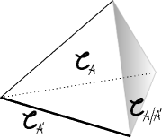
Figure 15. A cone $\mathfrak{C}\subset\operatorname{Lie}\mathsf{A}$ induces a cone for each subtorus $\mathsf{A}^{\prime}$ and quotient torus $\mathsf{A}/\mathsf{A}^{\prime}$.

Correspondingly, we have a diagram of maps

(353)

The shape of this diagram explains why the following statement is known as the triangle lemma.

Proposition 354.

The diagram (353) commutes.

Proof.

Consider the composition

(355) $$\operatorname{Stab}_{\mathfrak{C}_{\mathsf{A}^{\prime}}}\circ\operatorname{Stab}_{\mathfrak{C}_{\mathsf{A}/\mathsf{A}^{\prime}}}\subset X\times X^{\mathsf{A}}\,.$$

It clearly satisfies the support and the normalization conditions, and so it is the degree condition (344) that needs to be checked. Further, by uniqueness of stable envelopes, it is enough to check the degree condition for a generic $1$-parameter subgroup with generator

$$\xi=\xi^{\prime}+\delta\xi\,,\quad\xi^{\prime}\in\mathfrak{C}_{\mathsf{A}^{\prime}},\,\,\delta\xi\in\mathfrak{C}_{\mathsf{A}/\mathsf{A}^{\prime}}\,,$$

where $\xi^{\prime}$ is generic and the perturbation

(356) $$\|\delta\xi\|\ll\|\xi^{\prime}\|$$

is small.

In order to check (344), we need to consider two cases. The first case is when $F_{2}$ and $F_{1}$ belong to different components of $X^{\mathsf{A}^{\prime}}$. In this case, the inequalities (344) are strict for the stable envelope $\operatorname{Stab}_{\mathfrak{C}_{\mathsf{A}^{\prime}}}$. In particular, they are strict for the $1$-parameter subgroup generated by $\xi^{\prime}$, and therefore still satisfied for a small perturbation $\xi$.

The second case is when $F_{2}$ and $F_{1}$ belong to the same component of $X^{\mathsf{A}^{\prime}}$. In this case, $\operatorname{Stab}_{\mathfrak{C}_{\mathsf{A}^{\prime}}}$ is multiplication by ${\Lambda}^{\!\raisebox{1.42262pt}{$\scriptscriptstyle\bullet$}}\!\left(N_{X^{\mathsf{A}^{\prime}},<0}\right)^{\vee}$, twisted by polarization terms. The corresponding terms cancel from both sides of (344), as does the $\mathsf{A}^{\prime}$-weight of the line bundle $\mathscr{L}$. The degree bounds thus follows from the degree bounds for $\operatorname{Stab}_{\mathfrak{C}_{\mathsf{A}/\mathsf{A}^{\prime}}}$. ∎

9.2.4.

Let two chambers $\mathfrak{C}_{\pm}$ share a face, that is, let them be separated by a codimension $1$ wall

$$w=\operatorname{Lie}\mathsf{A}^{\prime}\subset\operatorname{Lie}\mathsf{A}\,.$$

For fixed slope $\mathscr{L}$, we define the following R-matrix

$$R_{w} =\operatorname{Stab}_{\mathfrak{C}_{-}}^{-1}\,\circ\,\operatorname{Stab}_{\mathfrak{C}_{+}}\quad\in\operatorname{End}K(X^{\mathsf{A}})_{\textup{localized}}$$

(357) $$=\operatorname{Stab}_{w,-}^{-1}\,\circ\,\operatorname{Stab}_{w,+}\,,$$

where

$$\operatorname{Stab}_{w,\pm}:K(X^{\mathsf{A}})\to K(X^{\mathsf{A}^{\prime}})$$

are the stable envelopes for the quotient $\mathsf{A}/\mathsf{A}^{\prime}\cong\mathbb{C}^{\times}$. The equality of two lines in (357) follows from the triangle lemma. Note from (349) that the inverse of a stable envelope is the transpose of another stable envelope.

From (357) we observe:

1. the operator $R_{w}$ depends only on $X^{\mathsf{A}}\hookrightarrow X^{\mathsf{A}^{\prime}}$ and, in particular,

2. as a function of equivariant parameters in $\mathsf{A}$, it factors through $\mathsf{A}/\mathsf{A}^{\prime}$.

9.2.5.

Let $w_{1},w_{2},\dots$ be the walls intersecting in a given codimension 2 subspace of $\operatorname{Lie}\mathsf{A}$. We may put them in the natural cyclic ordering as in Figure 16

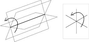
Figure 16. Product of wall $R$-matrices around a codimension 2 subspace is the identity

and then we have the following obvious

Proposition 358.

(359) $$\overset{\xleftarrow{\,\,\,\,}}{\prod}\,R_{w_{i}}=1\,.$$

In other words, R-matrices satisfy relations of the fundamental groupoid of the complement of the walls in $\operatorname{Lie}\mathsf{A}$.

9.2.6.

Fix a quiver, a framing vector $\mathsf{w}$ and define

$$X(\mathsf{w})=\bigsqcup_{\mathsf{v}}\textup{Nakajima variety}(\mathsf{v},\mathsf{w})$$

where $\mathsf{v}=(\dim V_{i})$ is the vector of ranks of tautological vector bundles and some choice of the stability parameter is understood. Let

$$\mathsf{A}=\{(a_{1},a_{2},a_{3})\}\cong\left(\mathbb{C}^{\times}\right)^{3}$$

act on the framing spaces and hence on $X$ so that

$$\mathsf{w}=\sum a_{i}\otimes\mathsf{w}^{(i)}$$

is the equivariant dimension vector.

Exercise 360.

Describe $X^{\mathsf{A}}$, the walls in $\operatorname{Lie}A$, and the corresponding fixed loci.

Exercise 361.

Show that the braid relation (359) becomes the following equation

(362) $$R_{12}(a_{1}/a_{2})R_{13}(a_{1}/a_{3})R_{23}(a_{2}/a_{3})=R_{23}(a_{2}/a_{3})R_{13}(a_{1}/a_{3})R_{12}(a_{1}/a_{2})$$

known as the Yang-Baxter equation with spectral parameter. This is an equation for operators

$$R_{ij}(a_{i}/a_{j})\in\operatorname{End}K(X(\mathsf{w}^{(i)}))\otimes K(X(\mathsf{w}^{(j)}))_{\textup{localized}}$$

acting in the respective factors of

$$K(X(\mathsf{w}^{(1)}))\otimes K(X(\mathsf{w}^{(2)}))\otimes K(X(\mathsf{w}^{(3)}))_{\textup{localized}}\,.$$

Exercise 363.

Show the following property

(364) $$R_{12}(a_{1}/a_{2})\,R_{21}(a_{2}/a_{1})=1\,,$$

known as the unitarity of $R$-matrices.

9.2.7.

In particular, take

(365) $$X=X(2)=\textup{pt}\sqcup T^{*}\mathbb{P}^{1}\sqcup\textup{pt}$$

for the quiver with one vertex and no loops. Stable envelopes for $T^{*}\mathbb{P}^{1}$ are a special case of the computation from Exercise 346, with the following result.

Let

$$\mathsf{A}=\operatorname{diag}(a_{1},a_{2})\subset GL(2)$$

act on $\mathbb{P}^{1}=\mathbb{P}(\mathbb{C}^{2})$ in the natural way. In particular, it acts with weights $a_{i}$ on the fibers of $\mathscr{O}(-1)$ over the fixed point $p_{i}\in X$.

Exercise 366.

Choose the parameters of stable envelopes as follows:

• the polarization $T^{1/2}$ is given by cotangent directions,

• the slope is $\mathscr{L}=\mathscr{O}(-\varepsilon)$, where $0<\varepsilon<1$,

• the chamber $\mathfrak{C}$ is such that $a_{1}/a_{2}\to 0$.

Then

$$\operatorname{Stab}_{\mathfrak{C}}(p_{1})=(1-a_{2}\mathscr{O}(1))\,\hbar^{1/2}\,,\quad\operatorname{Stab}_{\mathfrak{C}}(p_{2})=1-\hbar a_{1}\mathscr{O}(1)\,,$$

while

$$\operatorname{Stab}_{-\mathfrak{C}}(p_{1})=1-\hbar a_{2}\mathscr{O}(1)\,,\quad\operatorname{Stab}_{-\mathfrak{C}}(p_{2})=(1-a_{1}\mathscr{O}(1))\,\hbar^{1/2}\,,$$

is obtained by permuting the roles of $p_{1}$ and $p_{2}$.

Exercise 367.

Check that the computation of the $R$-matrix in the previous example gives

$$R_{T^{*}\mathbb{P}^{1}}(u)=\operatorname{Stab}_{-\mathfrak{C}}^{-1}\,\circ\,\operatorname{Stab}_{-\mathfrak{C}}=\begin{pmatrix}\hbar^{1/2}\,\dfrac{1-u}{\hbar-u}&u\,\dfrac{1-\hbar}{u-\hbar}\vspace{5pt}\\ \dfrac{1-\hbar}{u-\hbar}&\hbar^{1/2}\,\dfrac{1-u}{\hbar-u}\end{pmatrix}$$

where $u=a_{1}/a_{2}$. Together with the trivial blocks

$$R_{X(2)}=\begin{pmatrix}1\\ &R_{T^{*}\mathbb{P}^{1}}\\ &&1\end{pmatrix}$$

for the points in (365), this equates the $R$-matrix for $X(2)$ with the standard $R$-matrix for $\mathscr{U}_{\hbar}(\widehat{\mathfrak{gl}}(2))$, see [ES, ChariPress].

9.3. Actions of quantum group

9.3.1.

Let $\{F_{i}\}$ be a collection of vector spaces (or free modules over some more general rings) and

(368) $$R_{F_{i},F_{j}}(u)\in\operatorname{End}(F_{i}\otimes F_{j})\otimes\mathbb{C}(u)$$

a collection of invertible operators satisfying the Yang-Baxter equation (362). From this data, one can make a certain Hopf algebra $\mathscr{U}$ act on modules of the form

(369) $$F_{i_{1}}(a_{1})\otimes\dots\otimes F_{i_{n}}(a_{n})$$

where $F_{i}(a)$ is a shorthand for $F_{i}\otimes\mathbb{C}[a^{\pm 1}]$ and the order of factors in (369) is important.

The variables $a_{i}$ here are simply new indeterminates, unrelated to the structure of the algebra $\mathscr{U}$. The action of $\mathscr{U}$ in (369) is linear over functions of $a_{i}$. One should think of $a_{i}$ as points of $\mathbb{C}^{\times}$ at which the modules $F_{i}$ are inserted, and think of $\mathscr{U}$ as a deformation of a gauge Lie algebra

$$\mathscr{U}\approx\textup{Univ. enveloping}\left(\textup{Maps}(\mathbb{C}^{\times}\to\mathfrak{g})\right)\,,$$

where each $F_{i}$ is a module over the Lie algebra $\mathfrak{g}$.

9.3.2.

The definition of a Hopf algebra includes a coproduct, that is a coassociative homomorphism of algebras

$$\Delta:\mathscr{U}\mapsto\mathscr{U}\otimes\mathscr{U}\,.$$

A coproduct makes modules over $\mathscr{U}$ a tensor category. Familiar examples are a group algebra $\mathbb{C}G$ of a group $G$ or the universal enveloping algebra of a Lie algebra $\mathfrak{g}$. A group acts in tensor products via the diagonal homomorphism, meaning

$$\Delta:\mathbb{C}G\owns g\mapsto g\otimes g\in\mathbb{C}G\otimes\mathbb{C}G\,,$$

which by Leibniz rule gives

$$\Delta(\xi)=\xi\otimes 1+1\otimes\xi\quad\xi\in\operatorname{Lie}G\,.$$

In categories related to motives, in which

$$\otimes=\textup{Cartesian product of varieties}\,,$$

tensor product is similarly commutative.

By contrast, the coproduct for $\mathscr{U}$ will not be cocommutative, meaning that

$$\Delta^{\textup{opp}}=(12)\circ\,\Delta\neq\Delta\,,$$

and so the order of factors in the tensor product will be important.

9.3.3.

The coproduct will be not entirely noncommutative: after localization in $a$, tensor products in either order become isomorphic, that is

$$F_{1}(a_{1})\otimes F_{2}(a_{2})\otimes\mathbb{C}(a_{1}/a_{2})\cong F_{2}(a_{2})\otimes F_{1}(a_{1})\otimes\mathbb{C}(a_{1}/a_{2})$$

as $\mathscr{U}$ modules. In fact, the isomorphism is given by

(370) $$R^{\vee}_{F_{1}(a_{1}),F_{2}(a_{2})}=(12)\circ R_{F_{1},F_{2}}(a_{1}/a_{2})\,.$$

The same formula will work for general modules of the form (369), if we extend the definition of $R$-matrices as follows

$$R_{F_{1}(a_{1}),F_{2}(a_{2})\otimes F_{3}(a_{3})}=R_{F_{1}(a_{1}),F_{3}(a_{3})}\,R_{F_{1}(a_{1}),F_{2}(a_{2})}$$

and so on, see Figure 17 which illustrates the order in which the $R$-matrices should be multiplied.

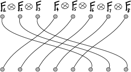
Figure 17. To write an $R$-matrix for two modules of the form (369), one multiplies $R$-matrices for factors in the order of crossings in the above diagram. Here, we get $R_{18}\cdots R_{24}R_{35}R_{34}$, where $R_{24}$ and $R_{35}$ can be places in arbitrary order.

Exercise 371.

Prove that so defined $R$-matrices satisfy the same braid relations of the form

$$R_{12}R_{13}R_{23}=R_{23}R_{13}R_{12}\,,$$

and the Yang-Baxter equation

$$R_{12}(u_{1}/u_{2})R_{13}(u_{1}/u_{3})R_{23}(u_{2}/u_{3})=R_{23}(u_{2}/u_{3})R_{13}(u_{1}/u_{3})R_{12}(u_{1}/u_{2})$$

if we make $u\in\operatorname{Aut}(\mathbb{C}^{\times})$ act on modules (369) by shifting all variables $a_{i}\mapsto ua_{i}$.

9.3.4.

Let $\mathbf{F}$ be a module of the form (369). The algebra $\mathscr{U}$ may be defined in a very down-to-earth way as the subalgebra

(372) $$\mathscr{U}\subset\prod_{\mathbf{F}}\operatorname{End}(\mathbf{F})$$

generated by matrix elements of

$$R_{\mathbf{F},F_{i}(u)}\in\operatorname{End}(\mathbf{F})\otimes\operatorname{End}(F_{i})\otimes\mathbb{C}(u)$$

in the auxiliary space $F_{i}$ for all $i$. Such matrix element is a rational function of $u$ with values in $\operatorname{End}(\mathbf{F})$ and we add to $\mathscr{U}$ the coefficients of the expansion of this rational function as both $u\to 0$ and $u\to\infty$. As the degrees of these rational functions are unbounded, there is no universal relations between these coefficients.

The natural projection

$$\prod_{\mathbf{F}}\operatorname{End}(\mathbf{F})\mapsto\prod_{\mathbf{F}_{1},\mathbf{F}_{2}}\operatorname{End}(\mathbf{F}_{1}\otimes\mathbf{F}_{2})$$

restricts to a map

$$\Delta:\mathscr{U}\mapsto\mathscr{U}\,\widehat{\otimes}\,\mathscr{U}$$

where the completion is required if the auxiliary spaces are infinite-dimensional, see the discussion in Section 5 of [59]. It is clear that $\Delta$ is a coassociative coproduct.

Exercise 373.

Show that (370) intertwines $\mathscr{U}$ action.

Geometrically defined $R$-matrices have an additional parameter, namely the slope. It can be shown [75] that the resulting algebra $\mathscr{U}$ does not depend on the slope. However, the ability to vary the slope is of significant help in analysis of the structure of $\mathscr{U}$.

9.3.5.

Among $\mathbf{F}$ in (372) we include the trivial representation $\mathbb{C}$ such that $R_{\mathbb{C},F}=1$ for any $F$.

Exercise 374.

Show that the induced map $\mathscr{U}\to\mathbb{C}$ is a counit for $\Delta$.

9.3.6.

In addition to a coproduct, a Hopf algebra has an anti-automorphism

$$S:\mathscr{U}\to\mathscr{U}$$

called the antipode, see [ES, ChariPress]. It satisfies

(375) $$m\circ(1\otimes S)\circ\Delta=m\circ(S\otimes 1)\circ\Delta=\textup{unit}\circ\textup{counit}$$

where $m:\mathscr{U}\otimes\mathscr{U}\to\mathscr{U}$ is the multiplication.

In applications, $S$ is invertible, even though invertibility of the antipode is not a part of the standard axioms. For the category of modules, the existence of the antipode means existence of dual modules.

For noncommutative $\otimes$, one has to distinguish between the left duals, with canonical maps

(376) $$F^{*}\otimes F\to\mathbb{C}\,,\quad\mathbb{C}\to F\otimes F^{*}\,,$$

and and the right duals, in which the order of tensor factors in (376) is reversed.

Exercise 377.

Show that the assignment

$$\mathscr{U}\owns x\mapsto S(x)^{*}\in\operatorname{End}(F^{*})\,,$$

where start denotes the transpose operator, makes vector space dual $F^{*}$ into a left-dual module for a Hopf algebra $\mathscr{U}$. Show that the inverse of $S$ is needed to make it a right-dual module.

9.3.7.

Following [Reshet], one can extend the collection (368) to dual spaces $F_{i}^{*}$ by the following rules

$$R_{F_{1}^{*},F_{2}} =\left(R_{F_{1},F_{2}}^{-1}\right)^{*_{1}}$$

(378) $$R_{F_{1},F_{2}^{*}} =\left(R_{F_{1},F_{2}}^{*_{2}}\right)^{-1}$$

$$R_{F_{1}^{*},F_{2}^{*}} =\left(R_{F_{1},F_{2}}\right)^{*_{12}}\,,$$

where $*_{1}$ means taking the transpose with respect to the first tensor factor, etc.

Exercise 379.

Show that the matrices (378) satisfy Yang-Baxter equations.

We can thus assume that the set $\mathbf{F}$ in (372) is closed under duals and define

$$S:\mathscr{U}\to\widehat{\mathscr{U}}$$

as the restriction of

$$\operatorname{End}(\mathbf{F})\xrightarrow{\quad*\quad}\operatorname{End}(\mathbf{F}^{*})\,.$$

Exercise 380.

Show this map satisfies the antipode axiom and that $\mathbf{F}^{*}$ is the left-dual module for $\mathscr{U}$.

10. Quantum Knizhnik-Zamolodchikov equations

10.1. Commuting difference operators from $R$-matrices

10.1.1.

Consider the group

$$\overline{W}=S(n)\ltimes\mathbb{Z}^{n}\subset\operatorname{Aut}(\mathbb{Z}^{n})$$

generated by shifts and permutation of the coordinates. It contains the affine Weyl group

$$W_{\textup{aff}}\subset\overline{W}$$

of type $A_{n-1}$ generated by $S(n)$ and the reflection

$$s_{0}\cdot(x_{1},\dots,x_{n})=(x_{n}+1,x_{2},\dots,x_{1}-1)$$

in the affine root

$$x_{1}-x_{n}=1\,.$$

Together with the simple positive roots of $A_{n-1}$, it delimits the fundamental alcove

(381) $$\dots\geq x_{n}+1\geq x_{1}\geq x_{2}\geq\dots\geq x_{n}\geq x_{1}-1\geq\dots\,.$$

This stabilizer of (381) in $\overline{W}$ is generated by the transformation

$$\pi\cdot(x_{1},\dots,x_{n})=(x_{n}+1,x_{1},\dots,x_{n-1})$$

that shifts all entries in (381) by one. Projected along the $(1,1,\dots,1)$-direction, this becomes the order $n$ outer symmetry of the Dynkin diagram of $\widehat{A}_{n-1}$. The group $\overline{W}$ is generated by $W_{\textup{aff}}$ and $\pi$ with the relations

(382) $$\pi s_{i}=s_{i+1}\pi\,,\quad i\in\mathbb{Z}/n\,.$$

In particular, we have the following expression for the shifts of the coordinates

(383) $$(1,0,\dots,0) =\pi\,s_{n-1}\dots s_{2}s_{1}\,,$$

(384) $$(0,1,\dots,0) =s_{1}\pi\,s_{n-1}\dots s_{2}\,,\quad\textup{etc.}$$

10.1.2.

Let $F_{i}$ be as in Section 9.3 and define

$$P=\bigoplus_{w\in S(n)}F_{w(1)}(a_{w(1)})\otimes\dots\otimes F_{w(n)}(a_{w(n)})\,.$$

Consider the $\mathscr{U}$-intertwiners in $P$ as in (370)

$$s_{k} =R^{\vee}_{k}$$

(385) $$=(k,k+1)\,R_{F_{w(k)},F_{w(k+1)}}(a_{w(k)}/a_{w(k+1)})\,\,$$

where $(k,k+1)$ permutes the $k$th and $(k+1)$st factors.

Exercise 386.

Deduce from (364) that the operators (385) form a representation of the symmetric group.

Let

$$G:F_{i}(a)\to F_{i}(a)$$

be an invertible operator such that

(387) $$\left[G\otimes G,R\right]=0\,.$$

Define

$$\pi=G_{1}\,(1,2,3,4\dots n)\,,$$

where $G_{1}$ means it acts in the first tensor factor.

Exercise 388.

Check this operator satisfies relations (382).

By analogy with (381), one can think of infinite quasi-periodic tensors of the form

$$\cdots\otimes Gf_{n}(a_{n})\otimes f_{1}(a_{1})\otimes f_{2}(a_{2})\otimes\cdots\otimes f_{n}(a_{n})\otimes G^{-1}f_{1}(a_{1})\otimes G^{-1}f_{2}(a_{2})\otimes\cdots\,.$$

The operator $\pi$ shifts this infinite tensor by one step. This operation occurs naturally in the study of spin chains with quasi-periodic boundary condition.

It follows that we get a representation of the group $S(n)\ltimes\mathbb{Z}^{n}$ and, in particular, $n$ commuting operators of the form

(389) (383) $$=G_{1}R_{1,n}\dots R_{12}\,,$$

(384) $$=R_{2,1}G_{2}R_{2,n}\dots R_{23}\,,\quad\textup{etc.}$$

10.1.3.

There are two ways to obtain an operator $G$ satisfying (387). The first is to take an element of $\mathscr{U}$ which is primitive, that is, satisfies

$$\Delta(G)=G\otimes G\,.$$

Quantum affine algebras have very few primitive elements. For Nakajima varieties the only nontrivial choice is an exponentials of linear functions of $\mathsf{v}$, which can be written as $z^{\mathsf{v}}$ in multiindex notation.

The other option is to introduce a shift operator,

$$\tau_{a,q}f(a)=f(qa)$$

which satisfies (387) because the $R$-matrix depends only on the ratio $a_{1}/a_{2}$ of evaluation parameters. Combining $z^{\mathsf{v}}$ with a shift operator in the form

$$Gf(a)=z^{\mathsf{v}}\,f(q^{-1}a)\,,$$

we get an action of $\mathbb{Z}^{n}$ by commuting difference operators.

The corresponding difference equations were introduced in [FrenResh] and are known as the quantum Knizhnik-Zamolodchikov equations. In the $q\to 1$ limit, they become the Knizhnik-Zamolodchikov differential equations for conformal blocks of WZW conformal field theories. See the book [EFK] for an introduction.

10.2. Minuscule shifts and qKZ

10.2.1.

We will identify the shifts of equivariant variable from Section 8.2 with qKZ operators in the case when the cocharacter $\sigma$ is minuscule. The parameters in the primitive element $z^{\mathsf{v}}$ will be identified, up to a shift, with Kähler variables.

Being minuscule is an important technical notion, and one of the equivalent ways to define a minuscule cocharacter is the following. Let $X_{0}$ be the affinization of $X$, that is, the spectrum of global functions on $X$. The ring $\mathbb{C}[X_{0}]=H^{0}(\mathscr{O}_{X})$ is $\mathbb{Z}$-graded by the characters of $\mathsf{A}$ and one can look for generators of minimal degree with respect to $\sigma$. By definition, $\sigma$ is minuscule if $\mathbb{C}[X_{0}]$ is generated by elements of degree $\{\pm 1,0\}$ with respect to $\sigma$.

For Nakajima varieties, $\mathbb{C}[X_{0}]$ is generated by invariant functions on the prequotient, and the first fundamental theorem of invariant theory provides a set of generators for it. It is shown in Section 2.6 of [59] that actions

$$\sigma:\mathbb{C}^{\times}\to\prod GL(W_{i})$$

with the character

$$\mathsf{w}=a\mathsf{w}^{\prime}+\mathsf{w}^{\prime\prime}\,,\quad a\in\mathbb{C}^{\times}\,,$$

are minuscule.

Exercise 390.

Check this.

Exercise 391.

Prove that the weights of a minuscule cocharacter $\sigma$ in the normal bundle to $X^{\sigma}$ are $\pm 1$.

10.2.2.

It is clear that the cocharacter $\sigma$ has to be very special for the shift operator to have the qKZ form. Indeed, the constructions of Section 8 produce difference operators as a formal series in $z$. For the shifts of Kähler variables it is shown in [75], as a consequence of commutation with qKZ, that the corresponding series converges to a rational function of $z$, up to an overall scalar.

By contrast, the qKZ operator are polynomial in $z$ and, in fact, they involve the variables $z$ only through the diagonal operator $z^{\mathsf{v}}$ acting in one of the tensor factors. The possibility to factor out the entire degree dependence in such a strong way is very special and is destroyed, for example, if we replace a difference operator by its square. Of course, $\sigma^{2}$ is never minuscule for $\sigma\neq 1$.

10.2.3.

Let $\sigma$ be a minuscule cocharacter and let $X^{\sigma}$ be the fixed locus on the corresponding $1$-parameter subgroup. The identification of geometric structures with structures from quantum groups happens in the basis of stable envelopes and, in particular, the shift operator $\mathbf{S}_{\sigma}$ will be identified with qKZ after conjugation by

(392) $$\operatorname{Stab}_{+,T^{1/2},\mathscr{L}}:K_{\mathsf{T}}(X^{\sigma})\to K_{\mathsf{T}}(X)$$

where plus means $\sigma$-attracting directions and

(393) $$\mathscr{L}\in\textup{\{neighborhood of $0$\}}\cap(-C_{\textup{ample}})\subset\operatorname{Pic}(X)\otimes\mathbb{R}\,.$$

We will see the importance of this particular choice of the slope $\mathscr{L}$ later.

10.2.4.

The conjugation of the shift operator to qKZ is summarized in the following diagram:

(394)

where $\operatorname{Stab}_{+}$ is the operator (392), followed by the restriction $\operatorname{Res}$ to fixed points, $R=\operatorname{Stab}_{-}^{-1}\operatorname{Stab}_{+}$ is the $R$-matrix, and

$$\tau_{\sigma}f(a)=f(q^{\sigma}a)\,.$$

Recall that the operators that shift equivariant variables are only defined after localization. In particular, to define the shift $\tau_{\sigma}$ we need to trivialize $K_{\mathsf{T}}(X)$ as a $K_{\mathbb{C}^{\times}_{q}}(\textup{pt})$-module. This is achieved by restriction to $K_{\mathsf{T}}(X^{\sigma})$.

In what follows, we will often drop the restriction to fixed points for brevity. To simplify notation, we will also denote by $a$ the coordinate in the image of $\sigma$ so that

$$\tau_{\sigma}f(a)=f(qa)\,.$$

10.2.5.

The inverse of the stable envelope may be replaced, as in Exercise 348, by the transposed correspondence with the opposite polarization, cone, and slope. Therefore, the diagram (394) is equivalent to the following

Theorem 395.

If $\sigma$ is a minuscule cocharacter then

(396) $$\operatorname{Stab}^{\textup{\tiny transp}}_{-,\,T^{1/2}_{\textup{opp}},\,-\mathscr{L}}\Big{|}_{a\mapsto q^{\sigma}a}\,\,\mathbf{S}_{\sigma}\,\,\operatorname{Stab}_{-,\,T^{1/2},\,\mathscr{L}}=(-1)^{\frac{1}{2}\operatorname{codim}X^{\sigma}}\,z^{\deg}$$

for all

$$\mathscr{L}\in\textup{\{neighborhood of $0$\}}\cap(-C_{\textup{ample}})\subset\operatorname{Pic}(X)\otimes\mathbb{R}\,.$$

The proof of this theorem will be given in Section 10.4

10.2.6.

For the following exercises we do not need to assume $\sigma$ minuscule.

Exercise 397.

Let the slope $\mathscr{L}$ be as (393). Show that the following limit exists and is a block-diagonal operator

$$\lim_{a\to 0}a^{\left\langle\det T^{1/2}_{>0},\sigma\right\rangle}\operatorname{Stab}_{+}=\textup{block-diagonal}\,.$$

As explained before, here $\operatorname{Stab}_{+}$ really means $\operatorname{Res}\circ\operatorname{Stab}_{+}$. Meanwhile,

$$\lim_{a\to 0}a^{\left\langle\det T^{1/2}_{>0},\sigma\right\rangle}\operatorname{Stab}_{-}=\textup{block-triangular}\,,$$

where the triangularity is the same as for $\operatorname{Stab}_{-}$.

Exercise 398.

Prove that

$$\operatorname{Stab}_{+}^{-1}\,\tau_{\sigma}^{-1}\,\operatorname{Stab}_{+}\to q^{\left\langle\det T^{1/2}_{>0},\sigma\right\rangle}\,\tau_{\sigma}^{-1}\,,\quad a\to 0\,.$$

Exercise 399.

Prove that

(400) $$R\to\hbar^{-\operatorname{codim}/4}\,\,\,\textup{block-unitriangular}\,,\quad a\to 0\,,$$

where the triangularity is the same as for $\operatorname{Stab}_{-}$.

10.2.7.

We will see in Section 10.3 that the following limit

(401) $$\mathsf{J}_{0,+}=\lim_{a\to 0}\operatorname{Stab}_{+}^{-1}\,\mathsf{J}(a)\,\operatorname{Stab}_{+}$$

exists, as does the limit of the operator $\mathbf{S}_{\sigma}$ in the stable basis. Again, this does not require the minuscule assumption. Granted this, we deduce from (319) the following analog of (299).

Proposition 402.

We have

(403) $$\mathsf{J}_{0,+}^{-1}\,\operatorname{Stab}_{+}^{-1}\,\mathbf{S}_{\sigma}\,\operatorname{Stab}_{+}\,\mathsf{J}_{0,+}\to(-\hbar^{1/2})^{\left\langle\det N_{<0},\sigma\right\rangle}\,q^{-\left\langle\det T^{1/2}_{>0},\sigma\right\rangle}\,z^{\deg}\,,$$

as $a\to 0$, where $N_{<0}$ is the subspace of the normal bundle to $X^{\sigma}$ spanned by weights that go to $\infty$ as $a\to 0$.

Proof.

Since

$$\Phi\big{(}(1-q\hbar)\big{(}T^{1/2}_{x,\sigma}-T^{1/2}_{x,0}\big{)}\big{)}\to(q\hbar)^{\left\langle\det T^{1/2}_{<0},\sigma\right\rangle}\,,\quad a\to 0\,,$$

we see that the operator $\mathsf{E}(\sigma)$ in (316) becomes

$$\mathsf{E}(\sigma)\to\textup{RHS of \eqref{S_to_0}}$$

in the $a\to 0$ limit. From Exercise 397,

$$\operatorname{Stab}_{+}^{-1}\,\mathsf{E}(\sigma)\,\operatorname{Stab}_{+}=\operatorname{Stab}_{+}^{-1}\,a^{-\left\langle\det T^{1/2}_{>0},\sigma\right\rangle}\,\mathsf{E}(\sigma)\,a^{\left\langle\det T^{1/2}_{>0},\sigma\right\rangle}\operatorname{Stab}_{+}\to\mathsf{E}(\sigma)\,,$$

as $a\to 0$, and so the conclusion follows from (316). ∎

Exercise 404.

Check that with the minuscule condition on $\sigma$ Corollary 402 specializes to

(405) $$\mathsf{J}_{0,+}^{-1}\,\operatorname{Stab}_{+}^{-1}\,\mathbf{S}_{\sigma}\,\operatorname{Stab}_{+}\,\mathsf{J}_{0,+}\to(-\hbar^{1/2})^{-\operatorname{codim}/2}\,q^{-\operatorname{rk}T^{1/2}_{>0}}\,z^{\deg}\,\quad a\to 0\,.$$

10.2.8.

From the above exercises we conclude that

$$\operatorname{Stab}_{+}^{-1}\,\tau_{\sigma}^{-1}\,\mathbf{S}_{\sigma}\,\operatorname{Stab}_{+}\to\tau_{\sigma}^{-1}\,\mathsf{J}_{0,+}\,(-\hbar)^{\operatorname{codim}/2}z^{\deg}\,\mathsf{J}_{0,+}^{-1}\,,$$

and thus the diagram (394) implies the following

Corollary 406.

The operator $\mathsf{J}_{0,+}$ diagonalizes $(-1)^{\operatorname{codim}/2}z^{\deg}R(0)$ and, in particular, is triangular with the same triangularity as $\operatorname{Stab}_{-}$.

10.3. Glue operator in the stable basis

10.3.1.

Let $T^{1/2}X$ be a polarization of $X$ and assume that the sheaf $\widehat{\mathscr{O}}_{\textup{vir}}$, and all K-theoretic curve counts, are defined using this polarization as in (201). Our next goal is to prove the following

Theorem 407.

The operator

$$\mathbf{G}_{\operatorname{Stab}} =\operatorname{Stab}^{-1}\,\,\mathbf{G}\,\,\operatorname{Stab}$$

(408) $$=\operatorname{Stab}^{\textup{\tiny transp}}_{-\mathfrak{C},\,T^{1/2}_{\textup{opp}},\,-\mathscr{L}}\,\,\mathbf{G}\,\,\operatorname{Stab}_{\mathfrak{C},\,T^{1/2},\,\mathscr{L}}$$

is independent of the equivariant parameters in $\mathsf{A}$ for any $\mathfrak{C}$ and for

(409) $$\mathscr{L}\in\textup{\{neighborhood of $0$\}}\subset\operatorname{Pic}(X)\otimes\mathbb{R}\,.$$

The proof takes several steps.

10.3.2.

As in Section 6.5.12, we see that the convolution in (408) is proper, thus a Laurent polynomial in $a\in\mathsf{A}$. To prove it is a constant, it suffices to check it has a finite limit as we send $a$ to infinity in any direction.

This can be done by equivariant localization.

10.3.3.

Suppose

$$f\in\left(\mathsf{QM}^{\text{\normalsize$\sim$}}_{\textup{relative $p_{1},p_{2}$}}\right)^{\mathsf{A}}\,,$$

and let $C^{\prime}$ be the domain of $f$. The curve $C^{\prime}$ a chain of $C^{\prime}_{i}\cong\mathbb{P}^{1}$. Since $f$ is fixed, there exists

(410) $$\gamma:\mathsf{A}\to\operatorname{Aut}(C^{\prime},p_{1}^{\prime},p_{2}^{\prime})\cong\prod_{C_{i}}\mathbb{C}^{\times}$$

such that

$$af=f\gamma(a)\,,\quad\forall a\in\mathsf{A}\,.$$

Let $p=C^{\prime}_{i}\cap C^{\prime}_{i+1}$ be a node of $C^{\prime}$. We say that $f$ is broken at $p$ if

(411) $$\textup{weight}_{\gamma}\left(T_{p}C^{\prime}_{i}\otimes T_{p}C^{\prime}_{i+1}\right)\neq 1\,.$$

This terminology comes from [OP1]. Since the space in (411) corresponds to the smoothing of node $p$ in $\operatorname{Def}(C^{\prime})$, this means that broken nodes contribute to the virtual normal bundle in (221), and namely

(412) $$N_{\textup{vir}}=N_{\textup{vir}}^{\textup{fixed domain}}+\bigoplus_{\begin{subarray}{c}\textup{broken}\\ \textup{nodes $p$}\end{subarray}}T_{p}C^{\prime}_{i}\otimes T_{p}C^{\prime}_{i+1}\,.$$

In localization formulas, this will give

$$\begin{matrix}[c]\textup{contribution of}\\ \textup{broken nodes}\end{matrix}\quad=\frac{1}{\prod(1-\textup{weight}\otimes\textup{line bundle})}$$

and this remains bounded as $a$ goes to any infinity of the torus avoiding the poles.

10.3.4.

By Lemma 198, we have

(413) $$N_{\textup{vir}}^{\textup{fixed domain}}=T^{1/2}_{f(p_{1}),\textup{moving}}+T^{1/2}_{f(p_{2}),\textup{moving}}+\dots$$

where

$$T^{1/2}_{f(p_{1}),\textup{moving}}=T^{1/2}_{f(p_{1}),\neq 0}$$

is the part of the polarization with nontrivial $\mathsf{A}$-weights and dots stand for balanced K-theory class as in Definition 200. These omitted term will contribute

$$\widehat{\mathsf{a}}(\dots)=O(1)\,,\quad a\to\infty\,,$$

to the localization formulas, so it remains to deal with the polarization.

10.3.5.

By definition (224), we have

(414) $$\begin{matrix}[c]\textup{contribution of}\\ \textup{polarization}\end{matrix}\quad=\frac{1}{{\Lambda}^{\!\raisebox{1.42262pt}{$\scriptscriptstyle\bullet$}\,}_{\scriptscriptstyle{-}}T^{1/2}_{f(p_{1}),\textup{moving}}\,\left({\Lambda}^{\!\raisebox{1.42262pt}{$\scriptscriptstyle\bullet$}\,}_{\scriptscriptstyle{-}}T^{1/2}_{f(p_{2}),\textup{moving}}\right)^{\vee}}\,.$$

While a polarization is only a virtual vector space, we have

$$T^{1/2}_{f(p_{2}),\textup{moving}}=\left(T_{f(p_{2})}X\right)_{\textup{repelling}}+\dots$$

where dots stand for a balanced class which will shift the asymptotics of (414) by an overall weight.

10.3.6.

To find this overall shift by a weight, we may normalize the exterior algebras so that they are self-dual. This gives

$$\frac{1}{\left({\Lambda}^{\!\raisebox{1.42262pt}{$\scriptscriptstyle\bullet$}\,}_{\scriptscriptstyle{-}}T^{1/2}_{f(p_{2}),\textup{mov}}\right)^{\vee}}\propto\left(\frac{\det T^{1/2}_{f(p_{2}),\textup{mov}}}{\det T_{f(p_{2}),\textup{rep}}}\right)^{1/2}\frac{1}{\left({\Lambda}^{\!\raisebox{1.42262pt}{$\scriptscriptstyle\bullet$}\,}_{\scriptscriptstyle{-}}\left(T_{f(p_{2}),\textup{rep}}\right)\right)^{\vee}}$$

as $a\to\infty$, which precisely compensates the weights (344) of the restriction of a stable envelope to the fixed component containing $f(p_{2})$ for all slopes $\mathscr{L}$ sufficiently close to $0$.

For the contribution of polarization at $f(p_{1})$, the conclusion is the same, with the replacement

$$\det T^{1/2}_{f(p_{2}),\textup{mov}}\mapsto\det T^{-1/2}_{f(p_{1}),\textup{mov}}=\det T^{1/2,\textup{opp}}_{f(p_{1}),\textup{mov}}\,.$$

This concludes the proof of Theorem 407.

10.3.7.

Recall the shift operator $\mathbf{S}_{\sigma}$ defined in (314). One of its factors is the glue operator that was just discussed. As before, we assume that $\sigma$ is a cocharacter of $\mathsf{A}$, that is, the shift of equivariant weights is in a direction that preserves the symplectic form.

Corollary 415.

The operator

(416) $$\operatorname{Stab}_{\mathfrak{C},\,T^{1/2},\,\mathscr{L}}^{-1}\Big{|}_{a\mapsto q^{\sigma}a}\,\,\mathbf{S}_{\sigma}\,\,\operatorname{Stab}_{\mathfrak{C},\,T^{1/2},\,\mathscr{L}}\in\operatorname{End}K(X^{\mathsf{A}})_{\textup{localized}}$$

is bounded and invertible at any infinity of the torus $\mathsf{A}$ for any $\mathfrak{C}$ and for $\mathscr{L}$ as in (409).

The first factor in (314) is only defined using localization, and so (416) is really a rational function of the equivariant parameters. This Corollary implies the $q$-difference equation in the variables $a\in\mathsf{A}$ has regular singularities.

Also, since $\mathbf{S}_{\sigma}$ is really an operator in $K(X^{\mathsf{A}})$, the stable envelopes are really the compositions

$$K(X^{\mathsf{A}})\xrightarrow{\,\,\operatorname{Stab}\,\,}K(X)\xrightarrow{\,\,\textup{restriction}\,\,}K(X^{\mathsf{A}})\,,$$

and, in particular, it makes sense to shift the equivariant variables in stable envelopes. We have already seen this in in (396) above.

Proof.

Bounding the $\mathsf{A}$-weights is done as in the above argument. The key point is that as in Lemma 198 we have

$$T_{\textup{vir}}={H}^{\raisebox{1.42262pt}{$\scriptscriptstyle\bullet$}}\left(\mathscr{T}^{1/2}+\hbar^{-1}\,\left(\mathscr{T}^{1/2}\right)^{\vee}\right)$$

even for twisted quasimaps as long as $\sigma$ preserves the symplectic form.

The inverse of $\mathbf{S}_{\sigma}$ may be computed from $\mathbf{S}_{{}_{\sigma}}$, therefore the shift operators are both bounded and invertible at infinities of $\mathsf{A}$. ∎

10.3.8.

Exercise 417.

Prove the existence of the limit (401).

Exercise 418.

Show the triangularity of the operator $\mathsf{J}_{0,+}$ from Corollary 406 directly, by examining the contribution of the broken nodes in the $a\to 0$ limit.

10.4. Proof of Theorem 395

10.4.1.

We may assume that $\mathsf{A}$ is a $1$-dimensional torus with coordinate $a$ and that

$$\sigma:\mathbb{C}^{\times}_{q}\xrightarrow{\,\,\sim\,\,}\mathsf{A}$$

is an isomorphism. We write $qa$ in place of $q^{\sigma}a$.

The two-dimensional torus $\mathbb{C}^{\times}_{q}\times\mathsf{A}$ acts on the moduli spaces of twisted quasimaps. By construction, the group $\mathbb{C}^{\times}_{q}$ acts in the fiber of $\mathscr{V}$ at $p^{\prime}_{1}$ and does not act in the fiber of $\mathscr{V}$ at $p^{\prime}_{2}$, see Section 4.3.2.

10.4.2.

As discussed before, the pushforward in (396) is proper, therefore the left-hand side is a Laurent polynomial in $q$ and $a$. We analyze the behavior of this polynomial as $(q,a)$ go to different infinities of the torus $\mathbb{C}^{\times}_{q}\times\mathsf{A}$.

In order to prove (396), it suffices to show that the left-hand side remains bounded at all infinities and limits to the right-hand side as

(419) $$a\to\infty\,,\quad qa\to 0\,.$$

10.4.3.

Localization with respect to the $\mathbb{C}^{\times}_{q}$-action gives the following schematic formula

$$\mathbf{S}_{\sigma}=\mathsf{J}\big{|}_{a\mapsto qa}\circ\left|\textup{edge}\right|\circ\mathsf{J}^{\textup{\tiny transp}}\circ\mathbf{G}^{-1}\,,$$

where the edge operator is the operator associated with constant twisted quasimaps and

$$\mathsf{J}^{\textup{\tiny transp}}=\left|\textup{capping operator}\right|$$

is the operator with matrix coefficients (289).

We can thus factor the LHS of (396) as follows

(420) $$\textup{LHS of \eqref{sSs}}= \left(\operatorname{Stab}^{\textup{\tiny transp}}_{-,\,T^{1/2}_{\textup{opp}},\,-\mathscr{L}}\,\,\mathsf{J}\,\,\operatorname{Stab}_{+,\,T^{1/2},\,\mathscr{L}}\right)\Big{|}_{a\mapsto qa} \times$$

(421) $$\left(\operatorname{Stab}^{\textup{\tiny transp}}_{-,\,T^{1/2}_{\textup{opp}},\,-\mathscr{L}}\right)\Big{|}_{a\mapsto qa}\,\,\left|\textup{edge}\right|\,\,\operatorname{Stab}_{-,\,T^{1/2},\,\mathscr{L}}\quad \times$$

(422) $$\operatorname{Stab}^{\textup{\tiny transp}}_{+,\,T^{1/2}_{\textup{opp}},\,-\mathscr{L}}\,\,\mathsf{J}^{\textup{\tiny transp}}\,\mathbf{G}^{-1}\,\,\operatorname{Stab}_{-,\,T^{1/2},\,\mathscr{L}}\,.$$

We deal with each factor separately.

10.4.4.

Lemma 423.

The operator in the RHS of (420) is bounded at all infinities of $\mathbb{C}^{\times}_{q}\times\mathsf{A}$ and goes to $1$ at the point (419).

Proof.

We argue as in the proof of Theorem 407, now with the additional insertion of $\left(1-q^{-1}\psi_{p_{1}}\right)^{-1}$. Since $\mathsf{A}$ acts on tangents spaces to all fixed points with weights $0,\pm 1$, we conclude

$$\textup{weight}(\psi_{p_{1}})\in\{1,(qa)^{\pm 1}\}\,.$$

In every case,

$$\frac{1}{1-q^{-1}\,\textup{weight}(\psi_{p_{1}})}\to 0$$

at the point (419) and remains bounded at all other infinities. Thus in the limit (419) the accordions at $p_{1}$ are suppressed and the result follows. ∎

10.4.5.

Lemma 424.

The operator in (422) is bounded at all infinities of $\mathbb{C}^{\times}_{q}\times\mathsf{A}$ and goes to $1$ at the point (419).

Proof.

We argue as in the previous lemma, now with the insertion of $\left(1-q\psi_{p_{2}}\right)^{-1}$. We have

$$q\,\textup{weight}(\psi_{p_{2}})\in\{q,qa^{\pm 1}\}\,,$$

which goes to zero in the limit (419). Thus $\psi_{p_{2}}$ plays no role in this limit and

$$\mathsf{J}^{\textup{\tiny transp}}\,\mathbf{G}^{-1}\to\mathbf{G}\,\mathbf{G}^{-1}=1\,,$$

as was to be shown. ∎

10.4.6.

It remains to deal with the operator in (421). Let $f\equiv x$ be a constant map to $x\in F$. Since the weights of $\mathsf{A}$ in $T_{x}X$ are $\{0,\pm 1\}$, the virtual normal bundle at $f$ to the space of $\mathsf{A}$-fixed quasimaps is

(425) $$N_{\textup{vir}}=H^{0}(\mathscr{T}_{x,>0})=\left(T_{x,>0}X\right)\big{|}_{a\mapsto qa}+T_{x,>0}X\,,$$

where $T_{x,>0}X$ denotes the $\mathsf{A}$-attracting part of $T_{x}X$ and $\mathscr{T}_{x,>0}$ is the bundle of these spaces over the domain of the quasimap.

Therefore, the normal bundle contribution to $\mathscr{O}_{\textup{vir}}\otimes\mathscr{K}^{1/2}_{\textup{vir}}$, which appears in the denominator of the localization formula, precisely cancels with the contributions (343) from the diagonal part of stable envelopes, which appears in the numerators. The remaining factors in (342) combine with the polarization factors in (201) to give

(426) $$(-1)^{\operatorname{rk}N^{1/2,\textup{opp}}_{>0}+\operatorname{rk}N^{1/2}_{>0}}\frac{1}{(\det N^{1/2,\textup{opp}})\big{|}_{a\mapsto qa}\det N^{1/2}}\times\\ \left(\frac{\det N^{1/2}}{\det N^{1/2}\big{|}_{a\mapsto qa}}\right)^{1/2}=(-1)^{\frac{1}{2}\operatorname{codim}F}h^{\frac{1}{2}\operatorname{codim}F}$$

as the normal bundle contribution of the diagonal parts of stable envelopes. The factor with $\hbar$ disappears when we convert two-point invariants to operators as in (234). Together with the degree weight, this gives

$$\begin{matrix}[c]\textup{diagonal}\\ \textup{contributions}\end{matrix}\quad=(-1)^{\frac{1}{2}\operatorname{codim}F}z^{\deg}\,,$$

where the degree of the constant map was computed in (157) .

To suppress the off-diagonal contributions, we need that

(427) $$\operatorname{weight}_{qa}\frac{\mathscr{L}^{-1}\big{|}_{F_{2}}}{\mathscr{L}^{-1}\big{|}_{F_{1}}}\,\operatorname{weight}_{a}\frac{\mathscr{L}\big{|}_{F_{2}}}{\mathscr{L}\big{|}_{F^{\prime}_{1}}}\to 0\,,$$

in the limit (419) for any triple of components $F_{1},F^{\prime}_{1},F_{2}$ of the fixed locus such that

(428) $$F_{2}\subset\operatorname{Attr}^{f}_{-\mathfrak{C}}(F_{1}),\operatorname{Attr}^{f}_{-\mathfrak{C}}(F^{\prime}_{1})$$

and

$$(F_{1},F^{\prime}_{1})\neq(F_{2},F_{2})\,.$$

The condition (428) means there is a chain of torus orbits from $F_{1}$ and $F^{\prime}_{1}$ to $F_{2}$ and computing the degree of that chain of curves with respect to $\mathscr{L}^{-1}$ we see that (427) is satisfied if $\mathscr{L}^{-1}$ is ample.

This concludes the proof of Theorem 395.

References

- [1] M. Aganagic and A. Okounkov, Elliptic stable envelopes, arXiv:1604.00423. Arnol\cprimedV. I.Mathematical methods of classical mechanicsGraduate Texts in Mathematics60Translated from the 1974 Russian original by K. Vogtmann and A. Weinstein; Corrected reprint of the second (1989) editionSpringer-Verlag, New York199?xvi+516ISBN 0-387-96890-3@book{ArnMech, author = {Arnol{\cprime}d, V. I.}, title = {Mathematical methods of classical mechanics}, series = {Graduate Texts in Mathematics}, volume = {60}, note = {Translated from the 1974 Russian original by K. Vogtmann and A. Weinstein; Corrected reprint of the second (1989) edition}, publisher = {Springer-Verlag, New York}, date = {199?}, pages = {xvi+516}, isbn = {0-387-96890-3}} AtiyahM. F.BottR.A lefschetz fixed point formula for elliptic complexes. iAnn. of Math. (2)861967374–407ISSN 0003-486X@article{AB, author = {Atiyah, M. F.}, author = {Bott, R.}, title = {A Lefschetz fixed point formula for elliptic complexes. I}, journal = {Ann. of Math. (2)}, volume = {86}, date = {1967}, pages = {374–407}, issn = {0003-486X}} AtiyahMichaelHirzebruchFriedrichSpin-manifolds and group actionstitle={Essays on Topology and Related Topics (M\'emoires d\'edi\'es \`a Georges de Rham)}, publisher={Springer, New York}, 197018–28@article{AtHirz, author = {Atiyah, Michael}, author = {Hirzebruch, Friedrich}, title = {Spin-manifolds and group actions}, conference = {title={Essays on Topology and Related Topics (M\'emoires d\'edi\'es \`a Georges de Rham)}, }, book = {publisher={Springer, New York}, }, date = {1970}, pages = {18–28}} BalagovićMartinaDegeneration of trigonometric dynamical difference equations for quantum loop algebras to trigonometric casimir equations for yangiansComm. Math. Phys.33420152629–659ISSN 0010-3616@article{Bal, author = {Balagovi{\'c}, Martina}, title = {Degeneration of trigonometric dynamical difference equations for quantum loop algebras to trigonometric Casimir equations for Yangians}, journal = {Comm. Math. Phys.}, volume = {334}, date = {2015}, number = {2}, pages = {629–659}, issn = {0010-3616}} BehrendKaiCiocan-FontanineIonutHwangJunhoRoseMichaelThe derived moduli space of stable sheavesAlgebra Number Theory820144781–812ISSN 1937-0652@article{BCFHR, author = {Behrend, Kai}, author = {Ciocan-Fontanine, Ionut}, author = {Hwang, Junho}, author = {Rose, Michael}, title = {The derived moduli space of stable sheaves}, journal = {Algebra Number Theory}, volume = {8}, date = {2014}, number = {4}, pages = {781–812}, issn = {1937-0652}} BehrendK.FantechiB.The intrinsic normal coneInvent. Math.1281997145–88ISSN 0020-9910@article{BF, author = {Behrend, K.}, author = {Fantechi, B.}, title = {The intrinsic normal cone}, journal = {Invent. Math.}, volume = {128}, date = {1997}, number = {1}, pages = {45–88}, issn = {0020-9910}} BezrukavnikovRomanFinkelbergMichaelWreath macdonald polynomials and the categorical mckay correspondenceWith an appendix by Vadim VologodskyCamb. J. Math.220142163–190ISSN 2168-0930@article{BezF, author = {Bezrukavnikov, Roman}, author = {Finkelberg, Michael}, title = {Wreath Macdonald polynomials and the categorical McKay correspondence}, note = {With an appendix by Vadim Vologodsky}, journal = {Camb. J. Math.}, volume = {2}, date = {2014}, number = {2}, pages = {163–190}, issn = {2168-0930}} BezrukavnikovRomanFinkelbergMichaelSchechtmanVadimFactorizable sheaves and quantum groupsLecture Notes in Mathematics1691Springer-Verlag, Berlin1998x+287ISBN 3-540-64619-1@book{BFS, author = {Bezrukavnikov, Roman}, author = {Finkelberg, Michael}, author = {Schechtman, Vadim}, title = {Factorizable sheaves and quantum groups}, series = {Lecture Notes in Mathematics}, volume = {1691}, publisher = {Springer-Verlag, Berlin}, date = {1998}, pages = {x+287}, isbn = {3-540-64619-1}} BezrukavnikovR.KaledinD.Fedosov quantization in positive characteristicJ. Amer. Math. Soc.2120082409–438ISSN 0894-0347@article{BK, author = {Bezrukavnikov, R.}, author = {Kaledin, D.}, title = {Fedosov quantization in positive characteristic}, journal = {J. Amer. Math. Soc.}, volume = {21}, date = {2008}, number = {2}, pages = {409–438}, issn = {0894-0347}}
- [11] R. Bezrukavnikov and I. Losev, Etingof conjecture for quantized quiver varieties, arXiv:1309.1716. BezrukavnikovRomanMirkovićIvanRepresentations of semisimple lie algebras in prime characteristic and the noncommutative springer resolutionAnn. of Math. (2)17820133835–919ISSN 0003-486X@article{BM, author = {Bezrukavnikov, Roman}, author = {Mirkovi{\'c}, Ivan}, title = {Representations of semisimple Lie algebras in prime characteristic and the noncommutative Springer resolution}, journal = {Ann. of Math. (2)}, volume = {178}, date = {2013}, number = {3}, pages = {835–919}, issn = {0003-486X}} BorelArmandSerreJean-PierreLe théorème de riemann-rochFrenchBull. Soc. Math. France86195897–136ISSN 0037-9484@article{BS, author = {Borel, Armand}, author = {Serre, Jean-Pierre}, title = {Le th\'eor\`eme de Riemann-Roch}, language = {French}, journal = {Bull. Soc. Math. France}, volume = {86}, date = {1958}, pages = {97–136}, issn = {0037-9484}} BrosnanPatrickOn motivic decompositions arising from the method of białynicki-birulaInvent. Math.1612005191–111ISSN 0020-9910@article{Bros, author = {Brosnan, Patrick}, title = {On motivic decompositions arising from the method of Bia\l ynicki-Birula}, journal = {Invent. Math.}, volume = {161}, date = {2005}, number = {1}, pages = {91–111}, issn = {0020-9910}} CarlssonErikNekrasovNikitaOkounkovAndreiFive dimensional gauge theories and vertex operatorsEnglish, with English and Russian summariesMosc. Math. J.142014139–61, 170ISSN 1609-3321@article{CNO, author = {Carlsson, Erik}, author = {Nekrasov, Nikita}, author = {Okounkov, Andrei}, title = {Five dimensional gauge theories and vertex operators}, language = {English, with English and Russian summaries}, journal = {Mosc. Math. J.}, volume = {14}, date = {2014}, number = {1}, pages = {39–61, 170}, issn = {1609-3321}} CarlssonErikOkounkovAndreiExts and vertex operatorsDuke Math. J.161201291797–1815ISSN 0012-7094@article{CO, author = {Carlsson, Erik}, author = {Okounkov, Andrei}, title = {Exts and vertex operators}, journal = {Duke Math. J.}, volume = {161}, date = {2012}, number = {9}, pages = {1797–1815}, issn = {0012-7094}} Ciocan-FontanineIonuţKapranovMikhailDerived quot schemesEnglish, with English and French summariesAnn. Sci. École Norm. Sup. (4)3420013403–440ISSN 0012-9593@article{CF1, author = {Ciocan-Fontanine, Ionu{\c{t}}}, author = {Kapranov, Mikhail}, title = {Derived Quot schemes}, language = {English, with English and French summaries}, journal = {Ann. Sci. \'Ecole Norm. Sup. (4)}, volume = {34}, date = {2001}, number = {3}, pages = {403–440}, issn = {0012-9593}} Ciocan-FontanineIonuţKapranovMikhail M.Derived hilbert schemesJ. Amer. Math. Soc.1520024787–815ISSN 0894-0347@article{CF2, author = {Ciocan-Fontanine, Ionu{\c{t}}}, author = {Kapranov, Mikhail M.}, title = {Derived Hilbert schemes}, journal = {J. Amer. Math. Soc.}, volume = {15}, date = {2002}, number = {4}, pages = {787–815}, issn = {0894-0347}} Ciocan-FontanineIonuţKapranovMikhailVirtual fundamental classes via dg-manifoldsGeom. Topol.13200931779–1804ISSN 1465-3060@article{CF3, author = {Ciocan-Fontanine, Ionu{\c{t}}}, author = {Kapranov, Mikhail}, title = {Virtual fundamental classes via dg-manifolds}, journal = {Geom. Topol.}, volume = {13}, date = {2009}, number = {3}, pages = {1779–1804}, issn = {1465-3060}} Ciocan-FontanineIonuţKimBumsigMaulikDaveshStable quasimaps to git quotientsJ. Geom. Phys.75201417–47ISSN 0393-0440@article{CKM, author = {Ciocan-Fontanine, Ionu{\c{t}}}, author = {Kim, Bumsig}, author = {Maulik, Davesh}, title = {Stable quasimaps to GIT quotients}, journal = {J. Geom. Phys.}, volume = {75}, date = {2014}, pages = {17–47}, issn = {0393-0440}} ChariVyjayanthiPressleyAndrewA guide to quantum groupsCambridge University Press, Cambridge1994xvi+651ISBN 0-521-43305-3@book{ChariPress, author = {Chari, Vyjayanthi}, author = {Pressley, Andrew}, title = {A guide to quantum groups}, publisher = {Cambridge University Press, Cambridge}, date = {1994}, pages = {xvi+651}, isbn = {0-521-43305-3}} ChrissNeilGinzburgVictorRepresentation theory and complex geometryModern Birkhäuser ClassicsReprint of the 1997 editionBirkhäuser Boston, Inc., Boston, MA2010x+495ISBN 978-0-8176-4937-1@book{CG, author = {Chriss, Neil}, author = {Ginzburg, Victor}, title = {Representation theory and complex geometry}, series = {Modern Birkh\"auser Classics}, note = {Reprint of the 1997 edition}, publisher = {Birkh\"auser Boston, Inc., Boston, MA}, date = {2010}, pages = {x+495}, isbn = {978-0-8176-4937-1}} DemazureMichelA very simple proof of bott’s theoremInvent. Math.3319763271–272ISSN 0020-9910@article{Demaz, author = {Demazure, Michel}, title = {A very simple proof of Bott's theorem}, journal = {Invent. Math.}, volume = {33}, date = {1976}, number = {3}, pages = {271–272}, issn = {0020-9910}} EinLawrenceLazarsfeldRobertThe gonality conjecture on syzygies of algebraic curves of large degreePubl. Math. Inst. Hautes Études Sci.1222015301–313ISSN 0073-8301@article{EinLaz, author = {Ein, Lawrence}, author = {Lazarsfeld, Robert}, title = {The gonality conjecture on syzygies of algebraic curves of large degree}, journal = {Publ. Math. Inst. Hautes \'Etudes Sci.}, volume = {122}, date = {2015}, pages = {301–313}, issn = {0073-8301}} EtingofPavelSymplectic reflection algebras and affine lie algebrasEnglish, with English and Russian summariesMosc. Math. J.1220123543–565, 668–669ISSN 1609-3321@article{Et, author = {Etingof, Pavel}, title = {Symplectic reflection algebras and affine Lie algebras}, language = {English, with English and Russian summaries}, journal = {Mosc. Math. J.}, volume = {12}, date = {2012}, number = {3}, pages = {543–565, 668–669}, issn = {1609-3321}} EtingofPavel I.FrenkelIgor B.KirillovJr.Alexander A.Lectures on representation theory and knizhnik-zamolodchikov equationsMathematical Surveys and Monographs58American Mathematical Society, Providence, RI1998xiv+198ISBN 0-8218-0496-0@book{EFK, author = {Etingof, Pavel I.}, author = {Frenkel, Igor B.}, author = {Kirillov, Alexander A., Jr.}, title = {Lectures on representation theory and Knizhnik-Zamolodchikov equations}, series = {Mathematical Surveys and Monographs}, volume = {58}, publisher = {American Mathematical Society, Providence, RI}, date = {1998}, pages = {xiv+198}, isbn = {0-8218-0496-0}} EtingofPavelSchiffmannOlivierLectures on quantum groupsLectures in Mathematical Physics2International Press, Somerville, MA2002xii+242ISBN 1-57146-094-2@book{ES, author = {Etingof, Pavel}, author = {Schiffmann, Olivier}, title = {Lectures on quantum groups}, series = {Lectures in Mathematical Physics}, edition = {2}, publisher = {International Press, Somerville, MA}, date = {2002}, pages = {xii+242}, isbn = {1-57146-094-2}} EtingofP.VarchenkoA.Dynamical weyl groups and applicationsAdv. Math.1672002174–127ISSN 0001-8708@article{EV, author = {Etingof, P.}, author = {Varchenko, A.}, title = {Dynamical Weyl groups and applications}, journal = {Adv. Math.}, volume = {167}, date = {2002}, number = {1}, pages = {74–127}, issn = {0001-8708}} FantechiBarbaraGöttscheLotharRiemann-roch theorems and elliptic genus for virtually smooth schemesGeom. Topol.142010183–115ISSN 1465-3060@article{FG, author = {Fantechi, Barbara}, author = {G{\"o}ttsche, Lothar}, title = {Riemann-Roch theorems and elliptic genus for virtually smooth schemes}, journal = {Geom. Topol.}, volume = {14}, date = {2010}, number = {1}, pages = {83–115}, issn = {1465-3060}} FantechiBarbaraGöttscheLotharIllusieLucKleimanSteven L.NitsureNitinVistoliAngeloFundamental algebraic geometryMathematical Surveys and Monographs123Grothendieck’s FGA explainedAmerican Mathematical Society, Providence, RI2005x+339ISBN 0-8218-3541-6@collection{FDA, author = {Fantechi, Barbara}, author = {G{\"o}ttsche, Lothar}, author = {Illusie, Luc}, author = {Kleiman, Steven L.}, author = {Nitsure, Nitin}, author = {Vistoli, Angelo}, title = {Fundamental algebraic geometry}, series = {Mathematical Surveys and Monographs}, volume = {123}, note = {Grothendieck's FGA explained}, publisher = {American Mathematical Society, Providence, RI}, date = {2005}, pages = {x+339}, isbn = {0-8218-3541-6}} FeiginBorisFinkelbergMichaelFrenkelIgorRybnikovLeonidGelfand-tsetlin algebras and cohomology rings of laumon spacesSelecta Math. (N.S.)1720112337–361ISSN 1022-1824@article{FFFR, author = {Feigin, Boris}, author = {Finkelberg, Michael}, author = {Frenkel, Igor}, author = {Rybnikov, Leonid}, title = {Gelfand-Tsetlin algebras and cohomology rings of Laumon spaces}, journal = {Selecta Math. (N.S.)}, volume = {17}, date = {2011}, number = {2}, pages = {337–361}, issn = {1022-1824}} FrenkelI. B.ReshetikhinN. Yu.Quantum affine algebras and holonomic difference equationsComm. Math. Phys.146199211–60ISSN 0010-3616@article{FrenResh, author = {Frenkel, I. B.}, author = {Reshetikhin, N. Yu.}, title = {Quantum affine algebras and holonomic difference equations}, journal = {Comm. Math. Phys.}, volume = {146}, date = {1992}, number = {1}, pages = {1–60}, issn = {0010-3616}} FultonWilliamIntersection theoryErgebnisse der Mathematik und ihrer Grenzgebiete. 3. Folge. A Series of Modern Surveys in Mathematics [Results in Mathematics and Related Areas. 3rd Series. A Series of Modern Surveys in Mathematics]22Springer-Verlag, Berlin1998xiv+470ISBN 3-540-62046-XISBN 0-387-98549-2@book{Ful, author = {Fulton, William}, title = {Intersection theory}, series = {Ergebnisse der Mathematik und ihrer Grenzgebiete. 3. Folge. A Series of Modern Surveys in Mathematics [Results in Mathematics and Related Areas. 3rd Series. A Series of Modern Surveys in Mathematics]}, volume = {2}, edition = {2}, publisher = {Springer-Verlag, Berlin}, date = {1998}, pages = {xiv+470}, isbn = {3-540-62046-X}, isbn = {0-387-98549-2}} GaitsgoryD.Twisted whittaker model and factorizable sheavesSelecta Math. (N.S.)1320084617–659ISSN 1022-1824@article{Gaits, author = {Gaitsgory, D.}, title = {Twisted Whittaker model and factorizable sheaves}, journal = {Selecta Math. (N.S.)}, volume = {13}, date = {2008}, number = {4}, pages = {617–659}, issn = {1022-1824}} GinzburgVictorLectures on nakajima’s quiver varietiesEnglish, with English and French summariestitle={Geometric methods in representation theory. I}, series={S\'emin. Congr.}, volume={24}, publisher={Soc. Math. France, Paris}, 2012145–219@article{GinzNak, author = {Ginzburg, Victor}, title = {Lectures on Nakajima's quiver varieties}, language = {English, with English and French summaries}, conference = {title={Geometric methods in representation theory. I}, }, book = {series={S\'emin. Congr.}, volume={24}, publisher={Soc. Math. France, Paris}, }, date = {2012}, pages = {145–219}} GiventalAlexanderOn the wdvv equation in quantum -theoryDedicated to William Fulton on the occasion of his 60th birthdayMichigan Math. J.482000295–304ISSN 0026-2285@article{Giv, author = {Givental, Alexander}, title = {On the WDVV equation in quantum $K$-theory}, note = {Dedicated to William Fulton on the occasion of his 60th birthday}, journal = {Michigan Math. J.}, volume = {48}, date = {2000}, pages = {295–304}, issn = {0026-2285}} GiventalAlexanderTonitaValentinThe hirzebruch-riemann-roch theorem in true genus-0 quantum k-theorytitle={Symplectic, Poisson, and noncommutative geometry}, series={Math. Sci. Res. Inst. Publ.}, volume={62}, publisher={Cambridge Univ. Press, New York}, 201443–91@article{GivTon, author = {Givental, Alexander}, author = {Tonita, Valentin}, title = {The Hirzebruch-Riemann-Roch theorem in true genus-0 quantum K-theory}, conference = {title={Symplectic, Poisson, and noncommutative geometry}, }, book = {series={Math. Sci. Res. Inst. Publ.}, volume={62}, publisher={Cambridge Univ. Press, New York}, }, date = {2014}, pages = {43–91}} GraberT.PandharipandeR.Localization of virtual classesInvent. Math.13519992487–518ISSN 0020-9910@article{GP, author = {Graber, T.}, author = {Pandharipande, R.}, title = {Localization of virtual classes}, journal = {Invent. Math.}, volume = {135}, date = {1999}, number = {2}, pages = {487–518}, issn = {0020-9910}} Halpern-LeistnerDanielThe derived category of a git quotientJ. Amer. Math. Soc.2820153871–912ISSN 0894-0347@article{DHL, author = {Halpern-Leistner, Daniel}, title = {The derived category of a GIT quotient}, journal = {J. Amer. Math. Soc.}, volume = {28}, date = {2015}, number = {3}, pages = {871–912}, issn = {0894-0347}} HoriKentaroKatzSheldonKlemmAlbrechtPandharipandeRahulThomasRichardVafaCumrunVakilRaviZaslowEricMirror symmetryClay Mathematics Monographs1With a preface by VafaAmerican Mathematical Society, Providence, RI; Clay Mathematics Institute, Cambridge, MA2003xx+929ISBN 0-8218-2955-6@book{Mirror, author = {Hori, Kentaro}, author = {Katz, Sheldon}, author = {Klemm, Albrecht}, author = {Pandharipande, Rahul}, author = {Thomas, Richard}, author = {Vafa, Cumrun}, author = {Vakil, Ravi}, author = {Zaslow, Eric}, title = {Mirror symmetry}, series = {Clay Mathematics Monographs}, volume = {1}, note = {With a preface by Vafa}, publisher = {American Mathematical Society, Providence, RI; Clay Mathematics Institute, Cambridge, MA}, date = {2003}, pages = {xx+929}, isbn = {0-8218-2955-6}} IqbalAmerKozçazCanVafaCumrunThe refined topological vertexJ. High Energy Phys.200910069, 58ISSN 1126-6708@article{IKV, author = {Iqbal, Amer}, author = {Koz{\c{c}}az, Can}, author = {Vafa, Cumrun}, title = {The refined topological vertex}, journal = {J. High Energy Phys.}, date = {2009}, number = {10}, pages = {069, 58}, issn = {1126-6708}} IritaniHiroshiAn integral structure in quantum cohomology and mirror symmetry for toric orbifoldsAdv. Math.222200931016–1079ISSN 0001-8708@article{Iri, author = {Iritani, Hiroshi}, title = {An integral structure in quantum cohomology and mirror symmetry for toric orbifolds}, journal = {Adv. Math.}, volume = {222}, date = {2009}, number = {3}, pages = {1016–1079}, issn = {0001-8708}} KaledinDmitryDerived equivalences by quantizationGeom. Funct. Anal.17200861968–2004ISSN 1016-443X@article{Kal1, author = {Kaledin, Dmitry}, title = {Derived equivalences by quantization}, journal = {Geom. Funct. Anal.}, volume = {17}, date = {2008}, number = {6}, pages = {1968–2004}, issn = {1016-443X}} KaledinDmitryGeometry and topology of symplectic resolutionstitle={Algebraic geometry—Seattle 2005. Part 2}, series={Proc. Sympos. Pure Math.}, volume={80}, publisher={Amer. Math. Soc., Providence, RI}, 2009595–628@article{Kal2, author = {Kaledin, Dmitry}, title = {Geometry and topology of symplectic resolutions}, conference = {title={Algebraic geometry—Seattle 2005. Part 2}, }, book = {series={Proc. Sympos. Pure Math.}, volume={80}, publisher={Amer. Math. Soc., Providence, RI}, }, date = {2009}, pages = {595–628}} KollárJánosRational curves on algebraic varietiesErgebnisse der Mathematik und ihrer Grenzgebiete. 3. Folge. A Series of Modern Surveys in Mathematics [Results in Mathematics and Related Areas. 3rd Series. A Series of Modern Surveys in Mathematics]32Springer-Verlag, Berlin1996viii+320ISBN 3-540-60168-6@book{Koll, author = {Koll{\'a}r, J{\'a}nos}, title = {Rational curves on algebraic varieties}, series = {Ergebnisse der Mathematik und ihrer Grenzgebiete. 3. Folge. A Series of Modern Surveys in Mathematics [Results in Mathematics and Related Areas. 3rd Series. A Series of Modern Surveys in Mathematics]}, volume = {32}, publisher = {Springer-Verlag, Berlin}, date = {1996}, pages = {viii+320}, isbn = {3-540-60168-6}} KontsevichMaximEnumeration of rational curves via torus actionstitle={The moduli space of curves}, address={Texel Island}, date={1994}, series={Progr. Math.}, volume={129}, publisher={Birkh\"auser Boston, Boston, MA}, 1995335–368@article{Krat, author = {Kontsevich, Maxim}, title = {Enumeration of rational curves via torus actions}, conference = {title={The moduli space of curves}, address={Texel Island}, date={1994}, }, book = {series={Progr. Math.}, volume={129}, publisher={Birkh\"auser Boston, Boston, MA}, }, date = {1995}, pages = {335–368}} KricheverIgorObstructions to the existence of -actions. bordisms of branched coveringsRussianIzv. Akad. Nauk SSSR Ser. Mat.4019764828–844, 950ISSN 0373-2436@article{Kr1, author = {Krichever, Igor}, title = {Obstructions to the existence of $S\sp{1}$-actions. Bordisms of branched coverings}, language = {Russian}, journal = {Izv. Akad. Nauk SSSR Ser. Mat.}, volume = {40}, date = {1976}, number = {4}, pages = {828–844, 950}, issn = {0373-2436}} KricheverIgorGeneralized elliptic genera and baker-akhiezer functionsRussianMat. Zametki471990234–45, 158ISSN 0025-567Xjournal={Math. Notes}, volume={47}, date={1990}, number={1-2}, pages={132–142}, issn={0001-4346}, @article{Kr2, author = {Krichever, Igor}, title = {Generalized elliptic genera and Baker-Akhiezer functions}, language = {Russian}, journal = {Mat. Zametki}, volume = {47}, date = {1990}, number = {2}, pages = {34–45, 158}, issn = {0025-567X}, translation = {journal={Math. Notes}, volume={47}, date={1990}, number={1-2}, pages={132–142}, issn={0001-4346}, }} LeeY.-P.Quantum -theory. i. foundationsDuke Math. J.12120043389–424ISSN 0012-7094@article{Lee, author = {Lee, Y.-P.}, title = {Quantum $K$-theory. I. Foundations}, journal = {Duke Math. J.}, volume = {121}, date = {2004}, number = {3}, pages = {389–424}, issn = {0012-7094}} LevineM.PandharipandeR.Algebraic cobordism revisitedInvent. Math.1762009163–130ISSN 0020-9910@article{LevPand, author = {Levine, M.}, author = {Pandharipande, R.}, title = {Algebraic cobordism revisited}, journal = {Invent. Math.}, volume = {176}, date = {2009}, number = {1}, pages = {63–130}, issn = {0020-9910}} LiJunStable morphisms to singular schemes and relative stable morphismsJ. Differential Geom.5720013509–578ISSN 0022-040X@article{Li1, author = {Li, Jun}, title = {Stable morphisms to singular schemes and relative stable morphisms}, journal = {J. Differential Geom.}, volume = {57}, date = {2001}, number = {3}, pages = {509–578}, issn = {0022-040X}} LiJunA degeneration formula of gw-invariantsJ. Differential Geom.6020022199–293ISSN 0022-040X@article{Li2, author = {Li, Jun}, title = {A degeneration formula of GW-invariants}, journal = {J. Differential Geom.}, volume = {60}, date = {2002}, number = {2}, pages = {199–293}, issn = {0022-040X}} LiJunWuBaosenGood degeneration of quot-schemes and coherent systemsComm. Anal. Geom.2320154841–921ISSN 1019-8385@article{LiWu, author = {Li, Jun}, author = {Wu, Baosen}, title = {Good degeneration of Quot-schemes and coherent systems}, journal = {Comm. Anal. Geom.}, volume = {23}, date = {2015}, number = {4}, pages = {841–921}, issn = {1019-8385}} ManettiMarcoLectures on deformations of complex manifolds (deformations from differential graded viewpoint)Rend. Mat. Appl. (7)24200411–183ISSN 1120-7183@article{Man, author = {Manetti, Marco}, title = {Lectures on deformations of complex manifolds (deformations from differential graded viewpoint)}, journal = {Rend. Mat. Appl. (7)}, volume = {24}, date = {2004}, number = {1}, pages = {1–183}, issn = {1120-7183}} MaulikD.NekrasovN.OkounkovA.PandharipandeR.Gromov-witten theory and donaldson-thomas theory. iCompos. Math.142200651263–1285ISSN 0010-437X@article{mnop1, author = {Maulik, D.}, author = {Nekrasov, N.}, author = {Okounkov, A.}, author = {Pandharipande, R.}, title = {Gromov-Witten theory and Donaldson-Thomas theory. I}, journal = {Compos. Math.}, volume = {142}, date = {2006}, number = {5}, pages = {1263–1285}, issn = {0010-437X}} MaulikD.NekrasovN.OkounkovA.PandharipandeR.Gromov-witten theory and donaldson-thomas theory. iiCompos. Math.142200651286–1304ISSN 0010-437X@article{mnop2, author = {Maulik, D.}, author = {Nekrasov, N.}, author = {Okounkov, A.}, author = {Pandharipande, R.}, title = {Gromov-Witten theory and Donaldson-Thomas theory. II}, journal = {Compos. Math.}, volume = {142}, date = {2006}, number = {5}, pages = {1286–1304}, issn = {0010-437X}} MaulikD.OblomkovA.OkounkovA.PandharipandeR.Gromov-witten/donaldson-thomas correspondence for toric 3-foldsInvent. Math.18620112435–479ISSN 0020-9910@article{moop, author = {Maulik, D.}, author = {Oblomkov, A.}, author = {Okounkov, A.}, author = {Pandharipande, R.}, title = {Gromov-Witten/Donaldson-Thomas correspondence for toric 3-folds}, journal = {Invent. Math.}, volume = {186}, date = {2011}, number = {2}, pages = {435–479}, issn = {0020-9910}} MaulikDaveshOblomkovAlexeiQuantum cohomology of the hilbert scheme of points on -resolutionsJ. Amer. Math. Soc.22200941055–1091ISSN 0894-0347@article{MauObl, author = {Maulik, Davesh}, author = {Oblomkov, Alexei}, title = {Quantum cohomology of the Hilbert scheme of points on $\scr A\sb n$-resolutions}, journal = {J. Amer. Math. Soc.}, volume = {22}, date = {2009}, number = {4}, pages = {1055–1091}, issn = {0894-0347}}
- [59] D. Maulik and A. Okounkov, Quantum groups and quantum cohomology, arXiv:1211.1287.
- [60] D. Maulik and A. Okounkov, in preparation. MaulikD.PandharipandeR.A topological view of gromov-witten theoryTopology4520065887–918ISSN 0040-9383@article{MP_top, author = {Maulik, D.}, author = {Pandharipande, R.}, title = {A topological view of Gromov-Witten theory}, journal = {Topology}, volume = {45}, date = {2006}, number = {5}, pages = {887–918}, issn = {0040-9383}} NakajimaHirakuInstantons on ale spaces, quiver varieties, and kac-moody algebrasDuke Math. J.7619942365–416ISSN 0012-7094@article{Nak1, author = {Nakajima, Hiraku}, title = {Instantons on ALE spaces, quiver varieties, and Kac-Moody algebras}, journal = {Duke Math. J.}, volume = {76}, date = {1994}, number = {2}, pages = {365–416}, issn = {0012-7094}} NakajimaHirakuQuiver varieties and kac-moody algebrasDuke Math. J.9119983515–560ISSN 0012-7094@article{Nak2, author = {Nakajima, Hiraku}, title = {Quiver varieties and Kac-Moody algebras}, journal = {Duke Math. J.}, volume = {91}, date = {1998}, number = {3}, pages = {515–560}, issn = {0012-7094}} NakajimaHirakuQuiver varieties and finite-dimensional representations of quantum affine algebrasJ. Amer. Math. Soc.1420011145–238ISSN 0894-0347@article{Nak3, author = {Nakajima, Hiraku}, title = {Quiver varieties and finite-dimensional representations of quantum affine algebras}, journal = {J. Amer. Math. Soc.}, volume = {14}, date = {2001}, number = {1}, pages = {145–238}, issn = {0894-0347}}
- [65] Hiraku Nakajima, Towards a mathematical definition of Coulomb branches of -dimensional gauge theories, I arXiv:1503.03676. NekrasovNikita-Theory: chasing theoryEnglish, with English and French summariesStrings 04. Part IIC. R. Phys.620052261–269ISSN 1631-0705@article{Zth, author = {Nekrasov, Nikita}, title = {$\bold Z$-theory: chasing ${\germ m}/f$ theory}, language = {English, with English and French summaries}, note = {Strings 04. Part II}, journal = {C. R. Phys.}, volume = {6}, date = {2005}, number = {2}, pages = {261–269}, issn = {1631-0705}}
- [67] N. Nekrasov and A. Okounkov, Membranes and Sheaves, arXiv:1404.2323. NekrasovNikita A.ShatashviliSamson L.Supersymmetric vacua and bethe ansatzNuclear Phys. B Proc. Suppl.192/193200991–112ISSN 0920-5632@article{NS1, author = {Nekrasov, Nikita A.}, author = {Shatashvili, Samson L.}, title = {Supersymmetric vacua and Bethe ansatz}, journal = {Nuclear Phys. B Proc. Suppl.}, volume = {192/193}, date = {2009}, pages = {91–112}, issn = {0920-5632}} NekrasovNikita A.ShatashviliSamson L.Quantization of integrable systems and four dimensional gauge theoriestitle={XVIth International Congress on Mathematical Physics}, publisher={World Sci. Publ., Hackensack, NJ}, 2010265–289@article{NS2, author = {Nekrasov, Nikita A.}, author = {Shatashvili, Samson L.}, title = {Quantization of integrable systems and four dimensional gauge theories}, conference = {title={XVIth International Congress on Mathematical Physics}, }, book = {publisher={World Sci. Publ., Hackensack, NJ}, }, date = {2010}, pages = {265–289}} OkounkovAndreiRandom surfaces enumerating algebraic curvestitle={European Congress of Mathematics}, publisher={Eur. Math. Soc., Z\"urich}, 2005751–768@article{ECM, author = {Okounkov, Andrei}, title = {Random surfaces enumerating algebraic curves}, conference = {title={European Congress of Mathematics}, }, book = {publisher={Eur. Math. Soc., Z\"urich}, }, date = {2005}, pages = {751–768}} OkounkovA.PandharipandeR.Quantum cohomology of the hilbert scheme of points in the planeInvent. Math.17920103523–557ISSN 0020-9910@article{OP1, author = {Okounkov, A.}, author = {Pandharipande, R.}, title = {Quantum cohomology of the Hilbert scheme of points in the plane}, journal = {Invent. Math.}, volume = {179}, date = {2010}, number = {3}, pages = {523–557}, issn = {0020-9910}} OkounkovA.PandharipandeR.The local donaldson-thomas theory of curvesGeom. Topol.14201031503–1567ISSN 1465-3060@article{OP2, author = {Okounkov, A.}, author = {Pandharipande, R.}, title = {The local Donaldson-Thomas theory of curves}, journal = {Geom. Topol.}, volume = {14}, date = {2010}, number = {3}, pages = {1503–1567}, issn = {1465-3060}} OkounkovAndreiReshetikhinNikolaiCorrelation function of schur process with application to local geometry of a random 3-dimensional young diagramJ. Amer. Math. Soc.1620033581–603 (electronic)ISSN 0894-0347@article{OR1, author = {Okounkov, Andrei}, author = {Reshetikhin, Nikolai}, title = {Correlation function of Schur process with application to local geometry of a random 3-dimensional Young diagram}, journal = {J. Amer. Math. Soc.}, volume = {16}, date = {2003}, number = {3}, pages = {581–603 (electronic)}, issn = {0894-0347}} OkounkovAndreiReshetikhinNicolaiRandom skew plane partitions and the pearcey processComm. Math. Phys.26920073571–609ISSN 0010-3616@article{OR2, author = {Okounkov, Andrei}, author = {Reshetikhin, Nicolai}, title = {Random skew plane partitions and the Pearcey process}, journal = {Comm. Math. Phys.}, volume = {269}, date = {2007}, number = {3}, pages = {571–609}, issn = {0010-3616}}
- [75] A. Okounkov and A. Smirnov, Quantum difference equations for Nakajima varieties, arXiv:1602.09007. PalamodovV. P.Deformations of complex spacesRussiantitle={Current problems in mathematics. Fundamental directions, Vol.\ 10 (Russian)}, series={Itogi Nauki i Tekhniki}, publisher={Akad. Nauk SSSR, Vsesoyuz. Inst. Nauchn. i Tekhn. Inform., Moscow}, 1986123–221, 283@article{Pal, author = {Palamodov, V. P.}, title = {Deformations of complex spaces}, language = {Russian}, conference = {title={Current problems in mathematics. Fundamental directions, Vol.\ 10 (Russian)}, }, book = {series={Itogi Nauki i Tekhniki}, publisher={Akad. Nauk SSSR, Vsesoyuz. Inst. Nauchn. i Tekhn. Inform., Moscow}, }, date = {1986}, pages = {123–221, 283}}
- [77] R. Pandharipande and A. Pixton, Gromov-Witten/Pairs correspondence for the quintic 3-fold, arXiv:1206.5490. ReshetikhinN. Yu.Quasitriangular hopf algebras and invariants of linksRussianAlgebra i Analiz119892169–188ISSN 0234-0852journal={Leningrad Math. J.}, volume={1}, date={1990}, number={2}, pages={491–513}, issn={1048-9924}, @article{Reshet, author = {Reshetikhin, N. Yu.}, title = {Quasitriangular Hopf algebras and invariants of links}, language = {Russian}, journal = {Algebra i Analiz}, volume = {1}, date = {1989}, number = {2}, pages = {169–188}, issn = {0234-0852}, translation = {journal={Leningrad Math. J.}, volume={1}, date={1990}, number={2}, pages={491–513}, issn={1048-9924}, }} SegalGraemeThe representation ring of a compact lie groupInst. Hautes Études Sci. Publ. Math.341968113–128ISSN 0073-8301@article{Segal, author = {Segal, Graeme}, title = {The representation ring of a compact Lie group}, journal = {Inst. Hautes \'Etudes Sci. Publ. Math.}, number = {34}, date = {1968}, pages = {113–128}, issn = {0073-8301}} StanleyRichard P.Enumerative combinatorics. volume 1Cambridge Studies in Advanced Mathematics492Cambridge University Press, Cambridge2012xiv+626ISBN 978-1-107-60262-5@book{StEn, author = {Stanley, Richard P.}, title = {Enumerative combinatorics. Volume 1}, series = {Cambridge Studies in Advanced Mathematics}, volume = {49}, edition = {2}, publisher = {Cambridge University Press, Cambridge}, date = {2012}, pages = {xiv+626}, isbn = {978-1-107-60262-5}} TarasovV.VarchenkoA.Dynamical differential equations compatible with rational equationsLett. Math. Phys.7120052101–108ISSN 0377-9017@article{TV, author = {Tarasov, V.}, author = {Varchenko, A.}, title = {Dynamical differential equations compatible with rational $qKZ$ equations}, journal = {Lett. Math. Phys.}, volume = {71}, date = {2005}, number = {2}, pages = {101–108}, issn = {0377-9017}} Toledano LaredoValerioThe trigonometric casimir connection of a simple lie algebraJ. Algebra3292011286–327ISSN 0021-8693@article{TolCas, author = {Toledano Laredo, Valerio}, title = {The trigonometric Casimir connection of a simple Lie algebra}, journal = {J. Algebra}, volume = {329}, date = {2011}, pages = {286–327}, issn = {0021-8693}} ThomasonR. W.Une formule de lefschetz en -théorie équivariante algébriqueFrenchDuke Math. J.6819923447–462ISSN 0012-7094@article{Thomason, author = {Thomason, R. W.}, title = {Une formule de Lefschetz en $K$-th\'eorie \'equivariante alg\'ebrique}, language = {French}, journal = {Duke Math. J.}, volume = {68}, date = {1992}, number = {3}, pages = {447–462}, issn = {0012-7094}} VinbergÈ. B.PopovV. L.Invariant theoryRussiantitle={Algebraic geometry, 4 (Russian)}, series={Itogi Nauki i Tekhniki}, publisher={Akad. Nauk SSSR, Vsesoyuz. Inst. Nauchn. i Tekhn. Inform., Moscow}, 1989137–314, 315@article{VinPop, author = {Vinberg, {\`E}. B.}, author = {Popov, V. L.}, title = {Invariant theory}, language = {Russian}, conference = {title={Algebraic geometry, 4 (Russian)}, }, book = {series={Itogi Nauki i Tekhniki}, publisher={Akad. Nauk SSSR, Vsesoyuz. Inst. Nauchn. i Tekhn. Inform., Moscow}, }, date = {1989}, pages = {137–314, 315}} VoisinClaireGreen’s generic syzygy conjecture for curves of even genus lying on a surfaceJ. Eur. Math. Soc. (JEMS)420024363–404ISSN 1435-9855@article{Vois, author = {Voisin, Claire}, title = {Green's generic syzygy conjecture for curves of even genus lying on a $K3$ surface}, journal = {J. Eur. Math. Soc. (JEMS)}, volume = {4}, date = {2002}, number = {4}, pages = {363–404}, issn = {1435-9855}}