Quantum dynamics of relativistic bosons through nonminimal vector square potentials

Abstract

The dynamics of relativistic bosons (scalar and vectorial) through nonminimal vector square (well and barrier) potentials is studied in the Duffin-Kemmer-Petiau (DKP) formalism. We show that the problem can be mapped in effective Schrödinger equations for a component of the DKP spinor. An oscillatory transmission coefficient is found and there is total reflection. Additionally, the energy spectrum of bound states is obtained and reveals the Schiff-Snyder-Weinberg effect, for specific conditions the potential lodges bound states of particles and antiparticles.

1 Introduction

The pioneering works of Duffin [1], Kemmer [2, 3] and Petiau [4] (DKP) gave rise to a rich formalism, similar to Dirac theory, able to describe interactions of spin 0 and spin 1 bosons. Various additional couplings, impossible to be explored in conventional Klein-Gordon and Proca equations, gave rise to a large area of physical applications such as describing the scattering of mesons by nuclei [5, 6, 7], the dynamics of bosons in curved space-time [8] and noninertial effect of rotating frames [9], thermodynamic properties of bosons in noncommutative plane [10], all works involving spin 0 systems. Vector bosons in the expanding universe [11] and in an Aharonov-Bohm potential [12] are examples of applications to spin 1 systems. The Bose-Einstein condensate [13, 14], very special relativity [15], among others works, are applications for both spin systems.

The interest of one-dimensional potentials in DKP formalism has increased significantly in recent decades, because the simplicity of equations obtained provides great support for studying physical systems in higher dimensions. Among the potentials used, we can highlight the double-step potential [16, 17], the DKP oscillator [18, 19], the inversely linear background [20], the mixed minimal-nonminimal vector cusp potential [21].

In this spirit, the purpose of this article is to address the problem of scalar and vector bosons subjected to a nonminimal vector square (well and barrier) potential in the DKP formalism. We obtain a transmission coefficient that shows oscillatory behavior, where we can observe the resonance tunneling. Additionally, we obtain the energy spectrum of bound states by a simple and transparent way. We show that the eigenenergies obtained have great similarity to the problem of fermions in the same potential, already explored in the literature [22].

2 A review of DKP equation

The DKP equation for a free boson is given by [2] (in natural units, $\hbar=c=1$)

$$\left(i\beta^{\mu}\partial_{\mu}-m\right)\psi=0$$ (1)

where the matrices $\beta^{\mu}$ satisfy the algebra $\beta^{\mu}\beta^{\nu}\beta^{\lambda}+\beta^{\lambda}\beta^{\nu}\beta^{\mu}=g^{\mu\nu}\beta^{\lambda}+g^{\lambda\nu}\beta^{\mu}$ and the metric tensor is $g^{\mu\nu}=\,$diag$\,(1,-1,-1,-1)$. The conserved four-current is given by $J^{\mu}=\bar{\psi}\beta^{\mu}\psi$$/2$ where the adjoint spinor $\bar{\psi}$ is given by $\bar{\psi}=\psi^{\dagger}\eta^{0}$ with $\eta^{0}=2\beta^{0}\beta^{0}-1$. The correct use of nonminimal interactions in the DKP equation can be found in [23], where the continuity equation implies in conserved physical quantities.

With nonminimal vector interactions, the DKP equation can be written as [24],

$$\left(i\beta^{\mu}\partial_{\mu}-m-i[P,\beta^{\mu}]A_{\mu}\right)\psi=0$$ (2)

where $P$ is a projection operator ($P^{2}=P$ and $P^{\dagger}=P$) in such a way that $\bar{\psi}[P,\beta^{\mu}]\psi$ behaves like a vector under a Lorentz transformation as $\bar{\psi}\beta^{\mu}\psi$ does. If the potential is time-independent one can write $\psi(\vec{r},t)=\phi(\vec{r})\exp(-iEt)$, where $E$ is the energy of the boson, the DKP equation becomes

$$\left[\beta^{0}E+i\beta^{i}\partial_{i}-\left(m+i[P,\beta^{\mu}]A_{\mu}\right)\right]\phi=0$$ (3)

2.1 Scalar sector

For the scalar bosons, we use the representation for the $\beta^{\mu}$ matrices given by [25]

$$\beta^{0}=\begin{pmatrix}\theta&\overline{0}\\ \overline{0}^{T}&\mathbf{0}\end{pmatrix},\quad\beta^{i}=\begin{pmatrix}\widetilde{0}&\rho_{i}\\ -\rho_{i}^{T}&\mathbf{0}\end{pmatrix},\quad i=1,2,3$$ (4)

where

$$\ \theta = \begin{pmatrix}0&1\\ 1&0\end{pmatrix},\quad\rho_{1}=\begin{pmatrix}-1&0&0\\ 0&0&0\end{pmatrix}$$

$$\rho_{2} = \begin{pmatrix}0&-1&0\\ 0&0&0\end{pmatrix},\quad\rho_{3}=\begin{pmatrix}0&0&-1\\ 0&0&0\end{pmatrix}$$

$\overline{0}$, $\widetilde{0}$ and $\mathbf{0}$ are 2$\times$3, 2$\times$2 and 3$\times$3 zero matrices, respectively, while the superscript T designates matrix transposition. Here the projection operator can be written as [26] $P=\left(\beta^{\mu}\beta_{\mu}-1\right)/3=\mathrm{diag}\,(1,0,0,0,0)$. In this case $P$ picks out the first component of the DKP spinor. The five-component spinor can be written as $\psi^{T}=\left(\phi_{1},...,\phi_{5}\right)$ in such a way that the time-independent DKP equation for a boson constrained moves along the $X$-axis, restricting ourselves to potentials depending only on $x$, decomposes into

$$\left(\frac{d^{2}}{dx^{2}}+E^{2}-m^{2}+A_{0}^{2}-A_{1}^{2}+\frac{dA_{1}}{dx}\right)\phi_{1}=0$$ (6)

$$\phi_{2}=\frac{1}{m}\left(E+iA_{0}\right)\,\phi_{1}$$ (7)

$$\phi_{3}=\frac{i}{m}\left(\frac{d}{dx}+A_{1}\right)\phi_{1},\quad\phi_{4}=\phi_{5}=0$$ (8)

And the conserved currents have the form

$$J^{0}=\frac{E}{m}\,|\phi_{1}|^{2},\quad J^{1}=\frac{1}{m}\text{Im}\left(\phi_{1}^{\ast}\,\frac{d\phi_{1}}{dx}\right).$$ (9)

2.2 Vector sector

Using the representation of $\beta^{\mu}$ matrices for vector bosons, given by [27]:

$$\beta^{0}=\begin{pmatrix}0&\overline{0}&\overline{0}&\overline{0}\\ \overline{0}^{T}&\mathbf{0}&\mathbf{I}&\mathbf{0}\\ \overline{0}^{T}&\mathbf{I}&\mathbf{0}&\mathbf{0}\\ \overline{0}^{T}&\mathbf{0}&\mathbf{0}&\mathbf{0}\end{pmatrix},\quad\beta^{i}=\begin{pmatrix}0&\overline{0}&e_{i}&\overline{0}\\ \overline{0}^{T}&\mathbf{0}&\mathbf{0}&-is_{i}\\ -e_{i}^{T}&\mathbf{0}&\mathbf{0}&\mathbf{0}\\ \overline{0}^{T}&-is_{i}&\mathbf{0}&\mathbf{0}\end{pmatrix}$$ (10)

where $s_{i}$ are the 3$\times$3 spin-1 matrices, $e_{i}$ are the 1$\times$3 matrices $\left(e_{i}\right)_{1j}=\delta_{ij}$ and $\overline{0}=\begin{pmatrix}0&0&0\end{pmatrix}$, while $\mathbf{I}$ and $\mathbf{0}$ designate the 3$\times$3 unit and zero matrices, respectively, the time-independent DKP equation (see Ref. [17]) can be written in the simpler form

$$\left(\frac{d^{2}}{dx^{2}}+k_{\sigma}^{2}\right)\phi_{I}^{\left(\sigma\right)}=0$$

$$\phi_{II}^{\left(\sigma\right)}=\frac{E+i\sigma A_{0}}{m}\,\phi_{I}^{\left(\sigma\right)}$$ (11)

$$\phi_{III}^{\left(\sigma\right)}=\frac{i}{m}\left(\frac{d}{dx}+\sigma A_{1}\right)\phi_{I}^{\left(\sigma\right)},\quad\phi_{8}=0$$

where

$$k_{\sigma}^{2}=E^{2}-m^{2}+A_{0}^{2}-A_{1}^{2}+\sigma\frac{dA_{1}}{dx}$$ (12)

and $\sigma$ is the polarization of vector boson states, i.e, $\sigma=-$ for transverse and $\sigma=+$ for longitudinal. In this representation, the projector is give by $P=\,\beta^{\mu}\beta_{\mu}-2=\mathrm{diag}\,(1,1,1,1,0,0,0,0,0,0)$ [28]. Now the components of the four-current are

$$J^{0}=\frac{E}{m}\sum\limits_{\sigma}|\phi_{I}^{\left(\sigma\right)}|^{2},\quad J^{1}=\frac{1}{m}\,\text{Im}\sum\limits_{\sigma}\phi_{I}^{\left(\sigma\right)\dagger}\,\frac{d\phi_{I}^{\left(\sigma\right)}}{dx}.$$ (13)

We can see, from ($11$) and ($12$), that the solution for vector sector consists in searching solutions for two Klein-Gordon-like equations for $\phi_{I}^{\left(\sigma\right)}$, but $\phi_{I}^{\left(+\right)}$and $\phi_{I}^{\left(-\right)}$ are not independents because $E$ is the constraint that appears in both equations. Cardoso and collaborators [29] had already alerted that the solutions for the spin 1 sector of the DKP equation, if they really exist, can be obtained from a restrict class of solutions of the spin 0 sector. There is not surprise because in the absence of any interaction, the free Proca fields obey a free Klein-Gordon equation with a constraint on the components of the Proca field.

3 The nonminimal vector square potentials

The square (well and barrier) potentials are given by

$$A_{\mu}(x) = b_{\mu}V_{0}g(x)\text{ \ with \ }\mu=0,1,$$ (14)

$$g(x) = \frac{1}{2}\left[sgn(x-a)-sgn(x+a)\right]$$ (15)

where $b_{\mu}V_{0}$ is a positive (negative) constant for wells (barriers) with energy dimension and $sgn(x)$ is the sign function.

3.1 Scalar bosons

With this potential, eq. (6) becomes

$$\frac{d^{2}\phi_{1}}{dx^{2}}+\left\{E^{2}-m^{2}+jV_{0}^{2}g(x)+\frac{b_{1}V_{0}}{2}\left[\delta\left(x-a\right)-\delta\left(x+a\right)\right]\right\}\phi_{1}=0$$ (16)

where $\delta\left(x\right)=d\theta\left(x\right)/dx$ is the Dirac delta function and $j\equiv b_{1}^{2}-b_{0}^{2}$. We turn our attention to scattering states so that the solutions describing spinless bosons coming from the left can be written as

$$\phi_{1}(x)=\left\{\begin{array}[]{cc}Ae^{+i\xi\frac{x}{a}}+Be^{-i\xi\frac{x}{a}}&\text{{for }}x<-a\\ &\\ Ce^{+i\eta\frac{x}{a}}+De^{-i\eta\frac{x}{a}}&\text{{for }}|x|<a\\ &\\ Fe^{+i\xi\frac{x}{a}}&\text{{for }}x>a\end{array}\right.$$ (17)

where

$$\xi=a\sqrt{E^{2}-m^{2}},\quad\eta=\sqrt{\xi^{2}-j\mathcal{\upsilon}^{2}},\quad\mathcal{\upsilon}=aV_{0}$$ (18)

The group velocity of the waves described above is given by

$$v_{g}=\frac{dE}{d(\xi/a)}=\pm\frac{\xi/a}{\sqrt{(\xi/a)^{2}+m^{2}}}$$ (19)

where the double signal is related to boson propagation direction.

Then, $\phi_{1}$ describes an incident wave moving to the right ($\xi$ is a real number) and a reflected wave moving to the left with

$$J^{1}\left(x<-a\right)=\frac{\xi}{am}\left(|A|^{2}-|B|^{2}\right)$$ (20)

and a transmitted wave moving to the right with

$$J^{1}\left(x>a\right)=\frac{\xi}{am}|F|^{2}$$ (21)

We demand $\phi_{1}$, to be continuous at $x=\pm a$, i. e.

$$\lim_{\varepsilon\rightarrow 0}\left.\phi_{1}\right|_{x=\pm a-\varepsilon}^{x=\pm a+\varepsilon}=0$$ (22)

and the connection formula between $d\phi_{1}/dx$ at the right and $d\phi_{1}/dx$ at the left can be summarized as

$$\lim_{\varepsilon\rightarrow 0}\left.\frac{d\phi_{1}}{dx}\right|_{x=\pm a-\varepsilon}^{x=\pm a+\varepsilon}=\mp\frac{b_{1}\mathcal{\upsilon}}{2a}\,\phi_{1}(\pm a).$$ (23)

Omitting the algebraic details, we obtain the following amplitudes

$$r = \frac{e^{-2i\xi}\left[if(\xi)-\gamma(\xi)\right]}{\cos(2\eta)-if(\xi)\sin(2\eta)}\sin(2\eta)$$

$$t = \frac{e^{-2i\xi}}{\cos(2\eta)-if(\xi)\sin(2\eta)}.$$

where we have defined

$$\gamma(\xi) \equiv \frac{vb_{1}+2i\xi}{2\eta},$$ (25)

$$f(\xi) \equiv \frac{4\left(\xi^{2}+\eta^{2}\right)+b_{1}^{2}v^{2}}{8\eta\xi}.$$ (26)

In order to determinate the reflection and transmission coefficients we use the charge current densities $J^{1}\left(x<-a\right)$ and $J^{1}\left(x>a\right)$. The $x$-independent current density allow us to define the reflection and transmission coefficients as

$$R=\left|r\right|^{2},\quad T=\left|t\right|^{2}$$ (27)

with $R+T=1$. Therefore,

$$R = \frac{|f(\xi)|^{2}+2i\mbox{Im}|\gamma(\xi)f^{*}(\xi)|+|\gamma(\xi)|^{2}}{1+\left[f(\xi)^{2}-1\right]\sin^{2}(2\eta)-i\sin(4\eta)\mbox{Im}\left[f(\xi)\right]}\sin^{2}(2\eta)\,,$$

$$T = \frac{1}{1+\left[f(\xi)^{2}-1\right]\sin^{2}(2\eta)-i\sin(4\eta)\mbox{Im}\left[f(\xi)\right]}$$

The figure 1 shows the profiles of reflection and transmission coefficients for $v=2,$ $j=b_{1}=1$. As expected, $T$ does not depend of sign of $b_{1}$. Notice that $T\rightarrow 1$ when

$$\eta=\frac{(N+1)\pi}{2}\text{, \ \ with \ \ }N=0,1,2,\ldots$$ (29)

and that there is a resonance transmission ($T=1$) whenever

$$\left|\xi\right|=\sqrt{\frac{(N+1)^{2}\pi^{2}}{4}+jv^{2}}.$$ (30)

Another expected result is $T\rightarrow 1$ when $E\rightarrow\pm\infty$, observed in the figure 1 (logically, there is a symmetry $E\rightarrow-E$ ).

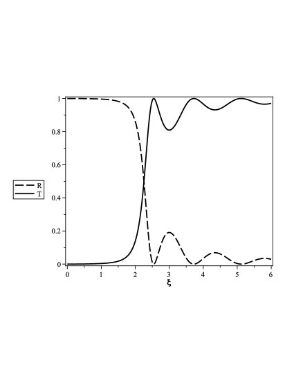
Figure 1: Reflection and transmission coefficients for $v=2$ and $m=1$.

We can observe a great similarity between $T$ for fermions [22] and bosons in the same potential, i.e, both do not depend on delta function localization and have the same resonance points. This is well understood because both have the same effective Schrödinger equations for spinor components in square potentials. However, there is no total reflection for fermions.

Additionally, we can obtain the bound state solutions with the prescription $\xi\rightarrow i\left|\xi\right|$ in the transmission amplitude. In this clear way, the bound state spectrum is obtained from poles of $t$, and the wave functions have the same form as (13) with $A=0$. As expected, there are bound state solutions just for $j<0$ and $b_{1}=1$, because the effective equation show a attractive potential between the two delta function potentials. It is like fermions bind by the same effective potential [22].

Therefore, for $j=-1$,

$$\frac{8\sqrt{v^{2}-\left|\xi\right|^{2}}}{5v^{2}-8\left|\xi\right|^{2}}\left|\xi\right|=\tan(2\sqrt{v^{2}-\left|\xi\right|^{2}})$$ (31)

is the quantization condition for the problem of bound scalar bosons by an effective well potential with attractive and repulsive deltas at the borders. The condition (27) can be solved by the graphical method and the numerical solutions are show in the figure 2. The nonminimal vector coupling is impossible in Klein-Gordon equation and we can observe this fact in the bound states spectrum. In the Ref. [30], the authors solve the minimally coupling Klein-Gordon equation with the same square potential, but the spectrum is completely different from the one obtained in this work. This reveals the great applicability of DKP formalism for describing physical systems with many coupling possibilities. The presence of delta functions at the borders has impact under the parity of the solutions, i.e, there is a symmetry breaking due to the delta potentials. The effective potential has no defined parity which implies in solutions without defined parity.

From the figure 2 we can see that the energy levels decay more rapidilly with the $v$ increasing. This can be explained by the limit $v\rightarrow\infty$, which provides that there are more bound states with the increase of depth well. However, in the limite case

$$V_{0}\rightarrow\infty\text{ \ and \ }a\rightarrow 0$$ (32)

we obtain just an atractive delta potential at the origin $x=0,$ which provides only one bound level [31]. In figure 3, we have the behaviour of $E$ in function of the lenght $a$ for $V_{0}/m=50$ (strong potential). In the limit $a\rightarrow 0,$ we can see the expected only one bound state level.

From figures 2 and 3 we can conclude that there is no Klein’s paradox for this configuration, i.e, particle levels penetrating in the antiparticle continuum region with the increasing of $V_{0}$ and $a$.

An interesting relativistic phenomena observed from bound state spectrum is the Schiff-Snyder-Weinberg (SSW) effect [32]. This effect occurs when an attractive well for particles in a critical depth lodges bound states of particles and antiparticles in the Klein-Gordon equation. Popov [33] suggests that the effect is characteristic of short-range and depth potentials. Our nonminimal vector potential, in the limits given by (28), contain all the characteristics to exhibit the SSW effect in the DKP formalism. From figures 2 and 3, we can see this phenomena because the spectrum is symmetrical with respect to $E$. We know that the minimally coupled case, the DKP equation reveals the SSW effect only with intense vector potential. However, in the nonminimal vector case, the SSW effect occurs independent of intensity potential. The explanation for this difference that makes our results be expected is that the DKP equation, in the presence of nonminimal vector interactions, is invariant under charge conjugation. Therefore, the square potential lodges bound states of particles and antiparticles, independent of intensity potential, as seen in figures 2 and 3.

3.2 Vector bosons

Vector bosons are subject to the effective potential

$$V_{eff}^{\sigma}(x)=\frac{1}{2m}\left(A_{1}^{2}-A_{0}^{2}-\sigma\frac{dA_{1}}{dx}\right),$$ (33)

which there is $\sigma-$dependence. However, for our problem, we can see that the polarization is only relate to the localization of delta functions at the borders of the square potential, i.e, if the delta potentials are attractive or repulsive. The results for scalar bosons does not depend on the position of delta functions. Therefore, the same results ($R$, $T$ and bound states spectrum) of scalar bosons are obtained for vector bosons subjected to the same square potential, for both possibilities $\sigma=\pm.$ We must remember that these results were expected since solutions for spin $1$ bosons can be obtained from spin $0$ bosons as pointed in [29].

The square potentials are simple models much explored in quantum physics books, for example [31]. Among various applications, L. Schiff [34] used a square well potential in the Klein-Gordon equation to bind the di-pions, providing a satisfactory account of the observed $P$-wave pion-pion scattering. In the Ref. [35], the authors used a square well potential as a model that allows calculating the phonon spectral function analytically in the nuclear magnetic resonance (NMR) relaxation. The authors were able to estimate an absolute value for the expected peak position of the NMR relaxation rate near the experimental data. An application of barrier potentials can be found in Ref. [36], where the authors studied the tunneling spectroscopy of collective excitations. Therefore, our results can be applied to all spinless bosons systems and the many couplings in the DKP formalism enable this.

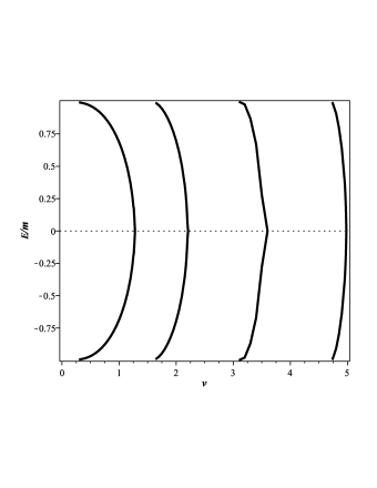
Figure 2: Energy levels of bound states.

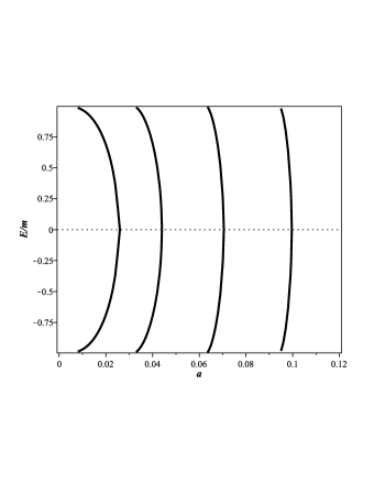
Figure 3: Energy levels in function of $a$ for $V_{0}=50$.

4 Conclusions

A physical system containing spinless bosons subject to the nonminimal vector square potentials is studied in the DKP formalism. The scattering states reveal an oscillatory transmission coefficient and the interesting particle problem embedded in a delta function is obtained. We can observe that there are bound state solutions only when the time component of square potential is more intense than its spatial component $(j<0)$. The energy bound states were obtained in a simple way from the poles of transmission amplitude. The parity of bound solutions is broken, similar to the fermions problem in the same potential which was already discussed in the literature [22]. The bound states spectrum reveals the Schiff-Snyder-Weinberg effect [32], confirming the Popov’s work [33] and its applicability to the DKP formalism. From a simple analysis, we can obtain the solutions for vector bosons from scalar bosons results.

References

- [1] R. J. Duffin, Phys. Rev. 54, 1114 (1938).
- [2] N. Kemmer, Proc. R. Soc. A 166, 127 (1938).
- [3] N. Kemmer, Proc. R. Soc. A 173, 91 (1939).
- [4] G. Petiau, Acad. R. Belg., A. Sci. Mém. Collect. 16, 2 (1936).
- [5] B. C. Clark et al., Phys. Rev. Lett. 55, 592 (1985).
- [6] R. C. Barret and Y. Nedjadi, Nucl. Phys. A 585, 311c (1995).
- [7] B. C. Clark et al., Phys. Lett. B 427, 231 (1998).
- [8] L. B. Castro, Eur. Phys. J. C 75, 287 (2015).
- [9] L. B. Castro, Eur. Phys. J. C 76, 61 (2016).
- [10] Z. Wang, Z. Long, C. Longand, W. Zhang, Advances in High Energy Physics 2015, Article ID 901675, (2015). http://dx.doi.org/10.1155/2015/901675
- [11] Y. Sucu and N. Unal, Eur. Phys. J. C 44, 287 (2005).
- [12] L. B. Castro and E. O. Silva, arXiv:1507.07790 (2015).
- [13] R. Casana, V. Y. Fainberg, B. M. Pimentel, J. S. Valverde, Phys. Lett. A 316, 33 (2003).
- [14] L. M. Abreu, A. L. Gadelha, B. M. Pimentel, E. S. Santos, Physica A: Statistical Mechanics and its Applications 419, 612 (2015).
- [15] R. M. T. Cavalcanti, J. M. Hoff da Silva, R. A. da Rocha, Eur. Phys. J. Plus 129, 246 (2014).
- [16] L. P. de Oliveira and A. S. de Castro, Can. J. Phys. 90, 481 (2012).
- [17] L. P. de Oliveira and A. S. de Castro, Int. J. Mod. Phys. E 24, 1550031 (2015).
- [18] D. A. Kulikov, R. S. Tutik, and A. P. Yaroshenko, Mod. Phys. Lett. A 20, 43 (2005).
- [19] L. B. Castro and A. S. de Castro, Phys. Lett. A 375, 2596 (2011).
- [20] A. S. de Castro, J. Math. Phys. 51, 102302 (2010).
- [21] A. S. de Castro, J. Phys. A 44, 035201 (2011).
- [22] L. P. de Oliveira and L. B. Castro, Ann. Phys. 364, 99 (2016).
- [23] L. B. Castro and L. P. de Oliveira, Advances in High Energy Physics 2014, Article ID 784072, (2014). http://dx.doi.org/10.1155/2014/784072
- [24] H. Umezawa, Quantum Field Theory. North-Holland, Amsterdam (1956).
- [25] Y. Nedjadi and R. C. Barret, J. Phys. G 19, 87 (1993).
- [26] R. F. Guertin and T. L. Wilson, Phys. Rev. D 15, 1518 (1977).
- [27] Y. Nedjadi and R. C. Barret, J. Math. Phys. 35, 4517 (1994).
- [28] B. Vijayalakshmi, M. Seetharaman, and P. M. Mathews, J. Phys. A 12, 665 (1979).
- [29] T. R. Cardoso, L. B. Castro and A. S. de Castro, J. Phys. A 43, 055306 (2010).
- [30] T. R. Cardoso and A. S. de Castro, Rev. Bras. Ens. Fís. 30, 2606 (2008).
- [31] D. J. Griffiths, Introduction to Quantum Physics, Pearson Prentice Hall, Upper Saddle River (2004).
- [32] L.I. Schiff, H. Snyder and J. Weinberg, Phys. Rev. 57, 315 (1940).
- [33] V.S. Popov, Sov. Phys. JETP 32, 526 (1971).
- [34] L. I. Schiff, Phys. Rev. 125, 777 (1962).
- [35] T. Dahm and K. Ueda, J. Phys. Chem. Solids 69, 3160 (2008).
- [36] A. J. Bennett, C. B. Duke and S. D. Silvertein, Phys. Rev 176, 969 (1968).