Exact sampling for some multi-dimensional queueing models with renewal input
Abstract
Using a result of Blanchet and Wallwater (2015: Exact sampling of stationary and time-reversed queues. ACM TOMACS, 25, 26) for exactly simulating the maximum of a negative drift random walk queue endowed with independent and identically distributed (iid) increments, we extend it to a multi-dimensional setting and then we give a new algorithm for simulating exactly the stationary distribution of a first-in-first-out (FIFO) multi-server queue in which the arrival process is a general renewal process and the service times are iid; the FIFO queue with . Our method utilizes dominated coupling from the past (DCFP) as well as the Random Assignment (RA) discipline, and complements the earlier work in which Poisson arrivals were assumed, such as the recent work of Connor and Kendall (2015: Perfect simulation of queues. Advances in Applied Probability, 47, 4). We also consider the models in continuous-time and show that with mild further assumptions, the exact simulation of those stationary distributions can also be achieved. We also give, using our FIFO algorithm, a new exact simulation algorithm for the stationary distribution of the infinite server case, the model. Finally, we even show how to handle Fork-Join queues, in which each arriving customer brings jobs, one for each server.
Keywords exact sampling; multi-server
queue; random walks; random assignment; dominated coupling from the past.
AMS Subject Classification: 65C05;
90B22; 60K25;60J05;60K05;68U20.
1 Introduction
In recent years, the method of exact simulation has evolved as a powerful way of sampling from stationary distributions of queueing models for which such distributions can not be derived explicitly. The main method itself is referred to as coupling from the past (CFP) as introduced in Propp and Wilson [18] for finite-state discrete-time Markov chains. Since then, the method has been generalized to cover general state space Markov chains by using dominating processes; this is known as dominated coupling from the past (DCFP) as in Kendall [16]. The main purpose of such methods is to produce a copy by simulation that exactly (not approximately) has the stationary distribution desired. These methods involve simulating processes backwards in time. In the present paper we consider using such methods for the FIFO multi-server queue, denoted as the FIFO queue, , where denotes the number of servers working in parallel, and arriving customers wait in one common queue (line).
The first algorithms yielding exact simulation in stationarity of the FIFO queue are [19] and [20], in which Poisson arrivals are assumed; i.e., the case. In [19], a DCFP method is used, but the strong condition of super stability is assumed, , instead of . (, where and denote an interarrival time and service time respectively; stability only requires that .) As a dominating process, the queue is used under Processor Sharing (PS) together (key) with its time-reversibility properties. In PS, there is no line; all customers are served simultaneously but at a rate when there are customers in service. Then in [20], the general case is covered by using a forward time regenerative method (a general method developed in [3]) and using the model under a random assignment (RA) discipline as an upper bound; a model in which each arrival joins the queue with probability independently. (The general forward-time regenerative method in [3] unfortunately always yields infinite expected termination time.) Then in [9], Connor and Kendall generalize the DCFP/PS method in [19] by using the RA model. They accomplish this by first exactly simulating the RA model in stationarity backwards in time under PS at each node, then re-constructing it to obtain the RA model with FIFO at each node and doing so in such a way that a sample-path upper bound for the FIFO is achieved.
As for renewal arrivals (the general FIFO queue considered here) the methods used above break down for various reasons, primarily because while under Poisson arrivals the stations under RA become independent, they are not independent for general renewal arrivals. Also, the time-reversibility property of PS no longer holds, nor does Poisson Arrivals See Time Averages (PASTA). Finally, under general renewal arrivals, the system may never empty once it begins operating. New methods are needed. Blanchet, Dong and Pei ([7]) solve the problem by utilizing a vacation model as an upper bound. In the present paper, however, we utilize DCFP by directly simulating the RA model in reverse-time (under FIFO at each node). Our method involves extending, to a multi-dimensional setting, a recent result of Blanchet and Wallwater ([8]) for exactly simulating the maximum of a negative drift random walk endowed with iid increments. We also remark on how our approach can lead to new results for other models too, such as multi-server queues under the last-in-first-out (LIFO) discipline, or the randomly choose next discipline, and even Fork-Join models (also called split and match models).
2 The FIFO model
Here we set up the classic first-in-first-out (of queue/line) (FIFO) multi-server queueing model and its associated Markov chain known as the Kiefer-Wolfowitz workload vector (for further details, see for example, page 341 in Chapter 12 of [1], and the original paper [17]) In what follows, as input to a -server in parallel multi-server queue with , we have i.i.d. service times distributed as , with finite and non-zero mean . Independently, the arrival times () of customers to the model form a renewal process with i.i.d. interarrival times distributed as and finite non-zero arrival rate . The FIFO model has only one queue (line), and customers upon arrival join the end of the queue and then attend service at the station that becomes free first (just like a USA postoffice). Because of the FIFO assumption, the service time initiated for use by a server, , is used on the arrival (they arrive at time ), and so one could equivalently imagine/assume that is brought to the system by the arrival. In this equivalent form, we say that at time , the workload in the system has jumped upward by the amount . Each server is identical in that they process service times at rate . We let denote the Kiefer-Wolfowitz workload vector, defined recursively by
| (1) |
where , , places a vector in ascending order, and + takes the positive part of each coordinate. The vector shows, in ascending order, how much work at time each server will process from among all work in the system at that time not including . Letting denote the arriving customer, is the customer delay in queue (line) of , because the server with the least amount of work will be the first to empty in front of . Recursion (1) defines a -dimensional Markov chain due to the given i.i.d. assumptions. The great importance of the recursion is that it yields , which is thus a function of a Markov chain.
With stability condition , it is well known that converges in distribution as to a proper stationary distribution (hence so does ). Let denote this stationary distribution. Our main objective in the present paper is to provide a simulation algorithm for sampling exactly from .
3 The RA model
Given a -server queueing system, the random assignment model (RA) is the case when each of the servers forms its own FIFO single-server queue, and each arrival to the system, independent of the past, randomly chooses queue to join with equal probability . In the case, we refer to this as the RA model. The following is a special case of Lemma 1.3, Page 342 in [1]. (Such results and others even more general are based on [24], [12], and [13].)
Lemma 3.1
Let denote total number of customers in system at time for the FIFO model, and let denote total number of customers in system at time for the corresponding RA model in which both models are initially empty and fed with exactly the same input of renewal arrivals and iid service times . Assume further that for both models the service times are used by the servers in the order in which service initiations occur ( is the service time used for the such initiation). Then
| (2) |
The importance of Lemma 3.1 is that it allows us to jointly simulate versions of the two stochastic processes and while achieving a coupling such that (2) holds. In particular, whenever an arrival finds the RA model empty, the FIFO model is found empty as well. (But we need to impose further conditions if we wish to ensure that indeed the RA queue will empty with certainty.) Letting time be sampled at arrival times of customers, , we thus also have
| (3) |
In other words, the total number in system as found by the arrival is sample-path ordered as well. Note that for the FIFO model, the arriving customer initiates the service since FIFO means “First-In-Queue-First-Out-of-Queue” where by “queue” we mean the line before entering service. This means that for the FIFO model we can attach to upon arrival if we so wish when applying Lemma 3.1. For the RA model, however, customers are not served in the order they arrive. For example consider servers (system initially empty) and suppose is assigned to node 1 with service time , and also is assigned to node 1 (before departs) with service time . Meanwhile, before departs, suppose arrives and is assigned to the empty node 2 with service time . Then is used for the second service initiation. For RA, the service times in order of initiation are a random permutation of the originally assigned .
To use Lemma 3.1, it is crucial to simply let the server hand out service times one at a time when they are needed for a service initiation. Thus, customers waiting in a queue before starting service do not have a service time assigned until they enter service. In simulation terminology, this amounts to generating the service times in order of when they are needed.
One disadvantage of generating service times only when they are needed, is that it then does not allow workload111Workload (total) at any time is defined as the sum of all whole and remaining service times in the system at time . to be defined; only the amount of work in service. To get around this if need be, one can simply generate service times upon arrival of customers, and give them to the server to be used in order of service initiation. The point is that when arrives, the total work in system jumps up by the amount . But is not assigned to , it is assigned (perhaps later) to which ever customer initiates the service. This allows Lemma 3.1 to hold true for total amount of work in the system: If we let and denote total workload in the two models with the service times used in the manner just explained, then in addition to Lemma 3.1 we have
| (4) |
| (5) |
It is important, however, to note that what one can’t do is define workload at the individual nodes by doing this, because that forces us to assign to so that workload at the node that attends ( say) jumps by and enters service using ; that destroys the proper coupling needed to obtain Lemma 3.1. We can only handle the total (sum over all nodes) workload. In the present paper, our use of Lemma 3.1 is via a kind of reversal:
Lemma 3.2
Let be an iid sequence of service times distributed as G, and assign to in the RA model. Define as the service time used in the service initiation. Then is also iid distributed as G.
Proof : The key is noting that we are re-ordering based only on the order in which service times begin being used, not when they are completed (which would thus introduce a bias). The service time chosen for the next initiation either enters service immediately (e.g., is one that is routed to an empty queue by an arriving customer) or is chosen from among those waiting in lines, and all those waiting are iid distributed as . Let denote the time at which the service initiation begins. The value of the service time chosen (at time ) by a server is independent of the past service time values used before time , and is distributed as (the choice of service time chosen as the next to be used is not based on the value of the service time, only its position in the lines). Letting the index of the that is chosen, i.e., , it is this index (a random variable) that depends on the past, but the value is independent of since it is a new one. Thus the are iid distributed as .
The point of the above Lemma 3.2 is that we can, if we so wish, simulate the RA model by assigning to (to be used as their service time), but then assigning , i.e. , to in the FIFO model. By doing so the requirements of Lemma 3.1 are satisfied and (2), (3), (4) and (5) hold. Interestingly, however, it is not possible to first simulate the RA model up to a fixed time , and then stop and reconstruct the FIFO model up to this time : At time , there may still be RA customers waiting in lines and hence not enough of the have been determined yet to construct the FIFO model. But all we have to do, if need be, is to continue the simulation of the RA model beyond until enough have been determined to construct fully the FIFO model up to time .
4 Simulating exactly from the stationary distribution of the RA model
By Lemma 3.1, the RA queue, which shares the same arrival stream and same service times in the order of service initiations , will serve as a sample path upper bound (in terms of total number of customers in system and total workload) of the target FIFO queue. Independent of and , we let be an iid sequence of random variables from discrete uniform distribution on ; represents the choice that customer makes about which single-server queue to join under RA discipline. Let denote the workload vector as found by in the RA model, and for , is the waiting time of the if he chooses to join the FIFO single-server queue of server . So, and
| (6) |
These processes are dependent through the common arrival times (equivalently common interarrival times ) and the common random variables. Because of all the iid assumptions, forms a Markov chain. Define and , then we can express (6) in vector form as
| (7) |
uses the same interarrival times and service times as we fed in (1), however the coordinates of are not in ascending order, though all of them are nonnegative.
Each node as expressed in (6) can be viewed as a FIFO queue with common renewal arrival process , but with iid service times . Across , the service times are not independent, but they are identically distributed: marginally, with probability , is distributed as , and with probability it is distributed as the point mass at ; i.e., . The point here is that we are not treating node as a single-server queue endowed only with its own arrivals (a thinning of the sequence) and its own service times iid distributed as . Defining iid increments for , each node has an associated negative drift random walk with and
| (8) |
With , we define ; equivalently for all . Let denote a random variable with the limiting (stationary) distribution of as , it is well known (due to the iid assumptions) that has the same distribution as
for .
More generally, even when the increment sequence is just stationary ergodic, not necessarily iid (hence not time reversible as in the iid case), it is the backwards in time maximum that is used in constructing a stationary version of . We will need this backwards approach in our simulation so we go over it here; it is usually referred to as Loynes’ Lemma. We extend the arrival point process to be a two-sided point stationary renewal process
Equivalently, form iid interarrival times; forms a two-sided iid sequence.
Similarly, the iid sequences and are extended to be two-sided iid, and These extensions further allow two-sided extension of the iid increment sequences for , i.e.,
Then we define time-reversed (increments) random walks for , by and
| (9) |
A (from the infinite past) stationary version of denoted by is then constructed via
| (10) | ||||
| (11) | ||||
| (12) | ||||
| (13) |
for all .
By construction, the process , is jointly stationary representing a (from the infinite past) stationary version of , and satisfies the forward-time recursion (7):
| (14) |
Thus, by starting at and walking backwards in time, we have (theoretically) a time-reversed copy of the RA model. Furthermore, can be extended to include forward time via using the recursion further:
| (15) |
where for .
In fact once we have a copy of just , we can start off the Markov chain with it as initial condition and use (15) to obtain a forward in time stationary version .
The above “construction”, however, is theoretical. We do not yet have any explicit way of obtaining a copy of , let alone an entire from-the-infinite-past sequence . In Blanchet and Wallwater [8], a simulation algorithm is given that yields (when applied to each of our random walks), for each , a copy of for any desired including stopping times . We modify the algorithm so that it can do the simulation jointly across the systems, that is, we extend it to a multi-dimensional form.
In particular, it yields an algorithm for obtaining a copy of , as well as a finite segment (of length ) of a backwards in time copy of the RA model; , a stationary into the past construction up to discrete time .
Finite exponential moments are not required (because only truncated exponential moments are needed , which in turn allow for the simulation of the exponential tilting of truncated , via acceptance-rejection). To get finite expected termination time (at each individual node) one needs the service distribution to have finite moment slightly beyond : For some (explicitly known) ,
| (16) |
As our first case, we will be considering a stopping time such that . Before we give the definition of the stopping time , we introduce the main idea of our simulation algorithm.
Let us define the maximum of a sequence of vectors. Suppose we have , where with and , define
Next define, for , that
where are iid from discrete uniform distribution over , and independently are iid from distribution (as introduced in Section 2). Our goal is to simulate the stopping time such that , defined as
| (17) |
i.e. the first time walking in the past, that all coordinates of the workload vector are , jointly with . (By convention, the value of any empty sum of numbers is zero, i.e. .)
To ensure that , in addition to (stability), it is required that (see the proof of Theorem 2 in [22]), for which the most common sufficient conditions are that has unbounded support, , or has mass arbitrarily close to , . But as we shall show in Section 6, given we know that , we can assume without loss of generality that interarrival times are bounded. It is that assumption which makes the extension of [8] to a multidimensional form easier to accomplish. Then, we show (in Section 4.2 and Section 9) how to still simulate from even when . We do that in two different ways, one as sandwiching argument and the other involving Harris recurrent Markov chain regenerations.
4.1 Algorithm for simulating exactly from for the FIFO queue: The case
As mentioned earlier, we will assume that , so that the stable () RA and FIFO Markov chains (7) and (1) will visit 0 infinitely often with certainty. (That the RA model empties infinitely often when is proved for example in [22]). We imagine that at the infinite past , we start both (7) and (1) from empty. We construct the RA model forward in time, while using Lemma 3.2 for the service times for the FIFO model, so that Lemma 3.1 applies and we have it in the form of (3), for all up to and including at time , at which time both models are in stationarity. We might have to continue the construction of the RA model so that (distributed as ) can be constructed (e.g., enough service times have been initiated by the RA model for using Lemmas 3.1 and 3.2). Formally, one can theoretically justify the existence of such infinite from the past versions (that obey Lemma 3.1) – by use of Loynes’ Lemma. Each model (when started empty) satisfies the monotonicity required to use Loynes’ Lemma. In particular, noting that if and only if , we conclude that if at any time it holds that , then . By the Markov property, given that , the future is independent of the past for each model, or said differently, the past is independent of the future. This remains valid if is replaced by a stopping time (strong Markov property).
We outline the simulation algorithm steps as follows.
-
1.
Simulate with as defined in (17). If , go to next step. Otherwise, having stored all data, reconstruct forwards in time from (initially empty) until , using the recursion (14). During this forward-time reconstruction, re-define as the -th service initiation used by the RA model (i.e., we are using Lemma 3.2 to gather service times in the proper order to feed in the FIFO model, which is why we do the re-construction). If at time there have not yet been service initiations, then continue simulating the RA model out in forward time until finally there is a service initiation, and then stop. This will require, at most, simulating out to with . Take the vector and reset . Also, store the interarrival times , and reset .
-
2.
If , then set and stop. Otherwise use (1) with , recursively go forwards in time for steps until obtaining , by using the re-set service and interarrival times . Reset .
-
3.
Output .
Detailed simulation steps are discussed in Appendix (Section A.1). Let denote the total number of interarrival times and service times to simulate in order to detect the stopping time . The following proposition shows that our algorithm will terminate in finite expected time, i.e., . The proof is given in Section A.2.
Proposition 4.1
If , , and there exists some such that , then
4.2 A more efficient algorithm: sandwiching
In this section, we no longer even need to assume that . (Another method allowing for involving Harris recurrent regeneration is given later in Section 9.) Instead of waiting for the workload vector of the queue under RA discipline to become , we choose an “inspection time” for some to stop the backward simulation of the RA queue, then construct two bounding processes of the target FIFO queue and evolve them forward in time, using the same stream of arrivals and service time requirements (in the order of service initiations), until coalescence or time zero. In particular we let the upper bound process to be a FIFO queue starting at time with workload vector being , and let the lower bound process to be a FIFO queue starting at the same time from empty, i.e., with workload vector being .
Let denote the ordered (ascendingly) workload vector of the original FIFO queueing process, starting from the infinite past, evaluated at time . For , we define and to be the ordered (ascendingly) workload vectors of the upper bound and lower bound processes, initiated at the inspection time , evaluated at time . By our construction and Theorem 3.3 in [9],
and for all
where all the above inequalities hold coordinate-wise.
Note that we can evolve the ordered workload vectors of the two bounding processes as follows: for when ,
| (18) | ||||
Similarly let denote the number of customers in the original FIFO queueing process, starting from the infinite past, evaluated at time . For , we let and denote the number of customers in the upper and lower bound queueing processes respectively, both initiated at the inspection time , evaluated at time . If at some time , we observe that , then it must be true that and (because the ordered remaining workload vectors of two bounding processes can only meet when they both have idle servers). We call such time “coalescence time” and from then on we have full information of the target FIFO queue, hence we can continue simulate it forward in time until time .
However if coalescence does not happen by time , we can adopt the so-called “binary back-off” method by letting the arrival time be our new inspection time and redo the above procedure to detect coalescence. Theorem 3.3 in [9] ensures that for any
We summarize the sandwiching algorithm as follows.
-
1.
Simulate with all data stored.
-
2.
Use the stored data to reconstruct forward in time from until , using Equation (14), and re-define as the service initiation used by the RA model.
-
3.
Set and . Then use the same stream of interarrival times and service times to simulate , forward in time using Equation (18).
-
4.
If at some time we detect , set , , , where is the -th entry of vector . Then use the remaining interarrival times and service times to evolve the original FIFO queue forward in time until time , output and stop.
-
5.
If no coalescence is detected by time , set , then continue to simulate the backward RA process until -th arrival, i.e., , with all data stored. Go to Step 2.
Next we analyze properties of the coalescence time. Define
If at time we start an upper bound FIFO queue with workload vector being , and a lower bound FIFO queue with workload vector being , they will coalesce by time . Therefore if we simulate the RA system backwards in time to , we will be able to detect a coalescence. We next show that .
By stationarity we have that is equal in distribution to
hence .
Proposition 4.2
If and there exists some such that and , then
5 Continuous-time stationary constructions
For a stable FIFO queue, let denote stationary customer delay (time spent in queue (line)); i.e., it has the limiting distribution of as .
Independently, let denote a random variable distributed as the equilibrium distribution of service time distribution ,
| (19) |
where . Let denote total work in system at time ; the sum of all whole or remaining service times in the system at time . , and one can construct via
(It is to be continuous from the right with left limits.) Let denote stationary workload; i.e., it has the limiting distribution
| (20) |
The following is well known to hold (see Section 6.3 and 6.4 in [21], for example):
| (21) |
Letting denote the probability distribution of , and denote the point mass at , and denote convolution of distributions, this means that the distribution of can be written as a mixture
This leads to the following:
Proposition 5.1
For a stable FIFO queue, if is explicitly known, and one can exactly simulate from and , then one can exactly simulate from .
Proof :
-
1.
Simulate a Bernoulli r.v. B.
-
2.
If , then set . Otherwise, if , then: simulate and independently simulate a copy . Set . Stop.
Another algorithm requiring instead the ability to simulate from (equilibrium distribution of the interarrival-time distribution ) instead of follows from another known relation:
| (22) |
where and are independent (see, for example Equation (88) on Page 426 in [23]). Thus by simulating , and , simply set . Equation (22) extends analogously to the FIFO model, where our objective is to exactly simulate from the time-stationary distribution of the continuous-time Kiefer-Wolfowitz workload vector, , where it can be constructed via
It is to be continuous from the right with left limits; . Total workload , for example, is obtained from this via
Letting have the time-stationary distribution of as , and letting have the discrete-time stationary distribution and letting , and be independent, then
| (23) |
So once we have a copy of (distributed as ) from our algorithm in Section 4.1 or Section 4.2, we can easily construct a copy of as long as we can simulate from . Of course, if arrivals are Poisson then the distribution of is identical to that of by PASTA, but otherwise we can use (23).
5.1 Numerical Results
As a sanity check, we have implemented our perfect sampling algorithm in Matlab for the case of queue. We provide our implementation codes for both algorithms in the online appendix of this paper.
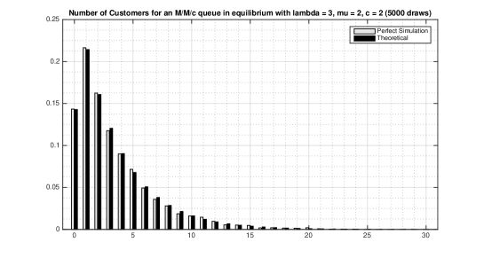
Firstly we consider queues, which are special cases of with . For the quantity of interest, number of customers in the FIFO queue at stationary, we obtain its empirical distribution from a large number of independent runs of our algorithm and compare it to the theoretical distribution which has a well-established closed form
where .
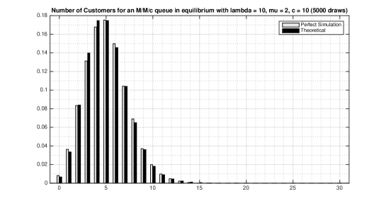
As an example, Figure 1 shows the result of such test when , and . Grey bars are the empirical results of draws using our algorithm, and black bars are the theoretical distribution number of customers in system from stationarity. A Pearson’s chi-squared test between the theoretical and empirical distributions gives a -value equal to , indicating close agreement (i.e., we cannot reject the null-hypothesis that there is no difference between these two distributions). For another set of parameters , and , the results are shown in Figure 2 with a -value being for the chi-squared fitness test.
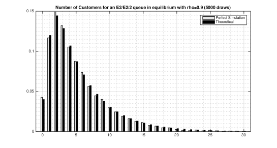
For the general queue when and when , we compare the empirical distribution of number of customers in system at stationarity, obtained from a large number of runs of our perfect sampling algorithm, to the numerical results (with precision at least ) provided in Table III of [15]. The results for an queue are given in Figure 3. Grey bars are the empirical results of draws using our algorithm and black bars are the numerical values given in [15], and they are very close to each other. The Pearson’s chi-squared test gives a -value of , thus we cannot reject the null-hypothesis that these two distributions agree well.
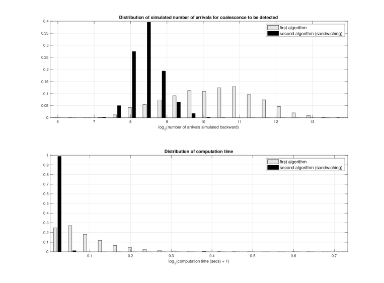
Next we run a numerical experiment comparing the computational efficiency of the first algorithm in Section 4.1 and the second sandwiching algorithm in Section 4.2. We measure the computational efficiency in two aspects. The first one is how far in the past we need to simulate the dominating process to detect coalescence (counting the total number of arrivals sampled backwards). The second aspect involves actual computation time in seconds. Figure 4 depicts such a comparison for an queue with parameters , , , from runs. Both results indicate that the second algorithm (sandwiching) is significantly more efficient than the first one.
Finally we study how the computational complexity of our sandwiching algorithm compares to the algorithm given in [7]. Notice these two algorithms look similar: they both use back-off strategies to run two bounding processes from some inspection time and check if they meet before time . The difference is that in [7] they use a so-called “vacation system” to construct upper bound process, whereas we use the same queue but under RA discipline instead. In the following numerical experiment, we define the computational complexity as the total number of arrivals each algorithm samples backwards to detect coalescence. Table 1 shows how they vary with traffic intensity, , based on independent runs of both algorithms using the same back-off strategy with same initial . The result suggests that our second algorithm (sandwiching) outperforms the one proposed in [7] as the magnitude of our computational complexity does not increase as fast as theirs when traffic intensity increases.
queue with fixed and
| confidence interval of number of arrivals simulated backwards | |||
|---|---|---|---|
| Algorithm in Section 4.2 | Algorithm in [7] | ||
| 5 | 0.5 | 54.8194 0.5758 | 146.5618 2.3598 |
| 6 | 0.6 | 86.5394 1.0536 | 308.4448 4.9413 |
| 7 | 0.7 | 152.6552 2.2695 | 730.1130 11.2783 |
| 8 | 0.8 | 337.9544 6.3021 | 2201.8254 32.1556 |
| 9 | 0.9 | 1521.3502 31.8267 | 12277.8686 161.5824 |
6 Why we can assume that interarrival times are bounded
Lemma 6.1
Consider the recursion
| (24) |
where both and are non-negative random variables, and .
Suppose for another sequence of non-negative random variables , it holds that
Then for the recursion
| (25) |
with , it holds that
| (26) |
Proof : The proof is by induction on : Because (w.p.1 in the following arguments) , we have
Now suppose the result holds for some . Then and by assumption ; hence
and the proof is complete.
Proposition 6.1
Consider the stable RA model in which . In order to use this model to simulate from the corresponding stationary distribution of the FIFO model as explained in the Section 4.1, without loss of generality we can assume that the interarrival times are bounded: There exists such that
Proof : By stability, , and by assumption . If the are not bounded, then for , define ; truncated . Choose sufficiently large so that and still holds. Now use the in place of the to construct an RA model, denoted by . Denote this by
where it satisfies the recursion (7) in the form
where .
Starting from , then from Lemma 6.1, it holds (coordinate-wise) that
and thus, if for some it holds that , then and hence (as explained in our previous section). Since was chosen ensuring that and , is a stable RA queue that will indeed empty infinitely often. Thus we can use it to do the backwards in discrete-time stationary construction until it empties, at time (say) ; . Then, we can re-construct the original RA model (starting empty at time ) using the (original untruncated) interarrival times in lieu of , so as to collect re-ordered needed in construction of for the FIFO model.
Remark 6.1
One would expect that the reconstruction of the original RA model in the above proof is unnecessary, that instead we only need to re-construct the model until we have service initiations from it, as opposed to service initiations from the original RA model. Although this might be true, the subtle problem is that the order in which service times are initiated in the model will typically be different than for the original RA model; they have different arrival processes (counterexamples are easy to construct). Thus it is not clear how one can utilize Lemma 3.1 and Lemma 3.2 and so on. One would need to generalize Lemma 3.1 to account for truncated arrival times used in the RA model, but not the FIFO model, in perhaps a form such as a variation of Equation (3),
| (27) |
where is the truncated renewal process. We did not explore this further.
7 Infinite server systems and other service disciplines
In this Section we sketch how one can utilize our FIFO results to obtain exact sampling of some other models including the infinite server queue, and the multi-server queue under other disciplines.
In [5] an exact simulation algorithm is presented for simulating from the stationary distribution of the infinite server queue; the . Here we sketch how to utilize our new FIFO results to accomplish this by using a FIFO model as an upper bound. The model has an infinite number of servers, there is no line, every arrival enters service immediately upon arrival; the customer arrives at time and departs at time .
For , this model is always stable. Let denote the smallest integer strictly larger than ; . Note that any can be chosen for this construction. A larger value of will result in a smaller number of arrivals necessary to detect coalescence, up to a certain point, since there will be less congestion in the bounding systems and the customers will leave faster. On the other hand, the actual simulation time may increase just as a consequence of simulating a dimensional random walk. We suggest a rule consistent with square-root staffing, , since this is well known to trade quality and capacity costs, which in our setting precisely translate to trading faster coalescence with cost-per-replication costs (see [14]).
Letting denote the total amount of work in the model, and denote the total amount of work in the (necessarily stable) FIFO model being fed exactly the same input (of service times and interarrival times), and both starting initially empty, the following is easily established:
| (28) |
hence
| (29) |
(Note that both models use the service times in the same order of initiation, which makes the coupling easy from the start.)
Thus, if, for example , then the FIFO model will empty and can be used to detect times when the model will empty. Let denote the total number of busy servers in the model as found by .
Simulating the FIFO model backwards in time in stationarity (using our previous algorithm), until it first empties, can then be used to detect a time when the model is empty, and then one can construct it back up to time to obtain a stationary copy of and of .
Now we consider alternatives disciplines to FIFO for the model. It is immediate that when service times are generated only when needed by a server, the total number of customers in the system process remains the same under FIFO as under last-in-first-out (LIFO) in which the next customer to enter service is the one at the bottom of the line, or random selection next (RS) in which the next customer to enter service from the line is selected at random by the server. Thus, they all share the same stationary distribution of as , as well as the stationary distribution of as . Let have this limiting (as ) distribution. This fact can be used to exactly simulate, for example, stationary delay under LIFO or RS (they are not the same as for FIFO). The method (sketch) is as follows: Simulate a copy of , jointly with the remaining service times of those in service, by assuming FIFO. This represents the distribution of the system as found in stationarity (at time ) by arrival . Consider RS for example. If the line is empty, then define ; enters service immediately. Otherwise, place in the line, and continue simulating but now using RS instead of FIFO. As soon as enters service, stop and define as that length of time.
8 Fork-Join Models
The RA recursion (7),
| (30) |
is actually a special case for the modeling of Fork-Join (FJ) queues (also called Split and Match) with nodes. In an FJ model, each arrival is a “job” with components, the component requiring service at the FIFO queue. So upon arrival at time , the job splits into its components to be served. As soon as all components have completed service, then and only then, does the job depart. Such models are useful in manufacturing applications. The job () thus arrives with a service time vector attached of the form . Let us assume that the vectors are iid, but otherwise each vector’s coordinates can have a general joint distribution; for then (30) still forms a Markov chain. We will denote this model as the model. The sojourn time of the component is given by , and thus the sojourn time of the job, , is given by
| (31) |
Of great interest is obtaining the limiting distribution of as ; we denote a r.v. with this distribution as . FJ models are notoriously difficult to analyze analytically: Even the special case of Poisson arrivals and i.i.d. exponential service times is non-trivial because of the dependency of the queues through the common arrival process. (A classic paper is Flatto [11]). In fact when , only bounds and approximations are available. As for exact simulation, there is a paper by Hongsheng Dai [10], in which Poisson arrivals and independent exponential service times are assumed. Because of the continuous-time Markov chain (CTMC) model structure, the author is able to construct (simulate) the time-reversed CTMC to use in a coupling from the past algorithm. But with general renewal arrivals and or general distribution service times, such CTMC methods no longer can be used.
Our simulation method for the RA model outlined in Section 4, however yields an exact copy of for the general model, under the condition that there exists , such that
First we simulate exactly using exponential change of measure method introduced in [4] (we use the same technique for multidimensional simulation in Algorithm 4.1), then simulate a vector of service times independently and set
Even when the service time components within are independent, or the case when service time distributions are assumed to have a finite moment generating function (in a neighborhood of the origin), such results are new and non-trivial.
9 The case when : Harris recurrent regeneration
For a stable FIFO queue, the stability condition can be re-written as , which implies also that . Thus assuming that is not necessary for stability. When , the system will never empty again after starting, and so using consecutive visits to as regeneration points is not possible. But the system does regenerate in a more general way via the use of Harris recurrent Markov chain theory; see [22] for details and history of this approach. The main idea is that while the system will not empty infinitely often, the number in system process will visit an integer infinitely often.
For illustration here, we will consider the case (for the general case the specific regeneration points analogous to what we present here are carefully given in Equation (4.6) on page 396 of [22]). Let assume that . (Note that if , then equivalently and so ; that is why we rule out here.) We now assume that . This implies that for and , we must have . It is shown in [22] that for sufficiently small, the following event will happen infinitely often (in ) with probability ,
| (32) |
If is such a time, then at time , we have
| (33) |
The point is that finds one server (server 1) empty, and the other queue with only one customer in it, and that customer is in service with a remaining service time . then enters service at node with service time ; but since , arrives finding the second queue empty, and the first server has remaining service time conditional on . Under the coupling of Lemma 3.1, the same will be so for the FIFO model (see Remark 9.1 below): At such a time ,
| (34) |
and at time we have
| (35) |
Equations (33) and (35) define positive recurrent regeneration points for the two models (at time ); the consecutive times at which regenerations occur form a (discrete-time) positive recurrent renewal process, see [22].
To put this to use, we change the stopping time given in (17) to:
| (36) | ||||
Then we do our reconstructions for the algorithm in Section 4.1 by starting at time , with both models starting with the same starting value
| (37) |
| (38) |
Remark 9.1
The service time used in (37) and (38) for coupling via Lemma 3.2, is in fact identical for both systems because (subtle): At time , both systems have only one customer in system, and thus total work is in fact equal to the remaining service time; so we use Equation (5) to conclude that both remaining service times (even if different) are (e.g., that is why (34) follow from (32)). Meanwhile, enters service immediately across both systems, so it is indeed the same service time used for both for this initiation. Coalescence is detected in finite expected time because of the positive recurrence property underlying the definition of the regeneration points from (33) and (35).
Appendix A Appendices
A.1 Detailed algorithm steps in Section 4.1
To simulate the process with the time defined in (17) as
we must sample the running time maxima (entry by entry) of the -dimensional random walk
We will find a sequence of random times such that . Hence, we will be able to find the running time maxima by only sampling the random walk on a finite time interval, i.e., is such that
To achieve this, we first decompose the random walk into two random walks and then construct a sequence of “milestone” events for each of these two random walks to detect ’s. We will elaborate the detailed implementations in the following context.
Because of the stability condition , we can find some value . For any , define
| (39) | ||||
| (40) |
hence and .
For all , let
| (41) | ||||
| (42) | ||||
| (43) |
Then, by the definitions above,
Therefore, to get the running-time maximum for each , we only need to sample the random walk from step to , because
Next we describe how to sample along with the multi-dimensional random walks and .
A.1.1 Simulation algorithm for the process
We first consider simulating the -dimensional random walk with . For each , , we can simulate the running time maximum jointly with the path via the method developed in [4], with the following assumptions.
Assumption (A1): There exits , such that
Assumption (A1b): Suppose that in every dimension , there exists such that
Because for each , are marginally identically distributed across , so would work for all .
Remark A.1
In our setting, since is bounded, assumption (A1) always holds. Assumption (A1b) is known as Cramer’s condition in the large deviations literature and it is a strengthening of assumption (A1). We shall explain briefly at the end of this section that it is possible to relax this assumption to (A1) by modifying the algorithm a bit without affecting the exactness/computational effort of the algorithm. For the moment we continue to describe the main algorithmic idea under assumption (A1b).
For any and define
| (44) | ||||
| (45) | ||||
| (46) |
We will use these definitions in Algorithm LTGM given in Section A.1.1.1.
We next construct a sequence of upward and downward “milestone” events for this multidimensional random walk. The construction is completely analogous to the classical ladder height decomposition of one dimensional random walks, we introduce a parameter, , in order to facilitate a certain acceptance / rejection step to be explained in the next subsection. Let
| (47) |
Define and . For , let
| (48) | ||||
| (49) |
Note that by convention, if for any . We let , initially set as , to be the running time upper bound of process . Let , where as defined in Section 2. From the construction of “milestone” events in (48) and (49), we know that if for some , the process will never cross over the level after coordinate-wise, i.e., for ,
Hence, in this case we update the upper bound vector .
A.1.1.1 Global maximum simulation
Define
| (50) |
By the construction of “milestone” events, for all
Hence, we can evaluate the global maximum level of the process to be
| (51) |
and we give the detailed sampling procedure in the following algorithm. The algorithm has elements, such as sampling from , which will be explained in the sequel.
Algorithm LTGM: simulate global maximum of
-dimensional process jointly with the sub-path
and the subsequence of “milestone” events.
Input: satisfies assumption (A1b), as in (47).
-
1.
(Initialization) Set , , , , and .
-
2.
Generate and let . Independently sample and let . Set , , and .
-
3.
If there is some such that , then go to Step 2; otherwise set and .
-
4.
Independently sample .
-
5.
If , simulate a new conditional path with , following the conditional distribution of given . Set , , for . Set , . Go to Step 2.
-
6.
If , set , and .
-
7.
Output , , and global maximum .
Now we explain how to execute Steps 4 and 5 in the previous algorithm. The procedure is similar to the multi-dimensional procedure given in [4], so we describe it briefly here. As denotes the canonical probability, we let . Our goal is to simulate from the conditional law of given that and , i.e., to simulate from . We will use acceptance/rejection by letting denote the proposal distribution. A typical element sampled under is of the form , where and it indicates the direction we pick to do exponential tilting; it is the coordinate in which we change its measure to increase the chance of its hitting the upward “milestone” as defined in (49). Given the value of , the process remains a random walk. We now describe by explaining how to sample . First,
| (52) |
Then, conditioning on , for every set ,
| (53) |
To obtain the induced distribution for and , we study the moment generating function induced by definition (53). Given in a neighborhood of the origin,
The previous expression indicates that under , and are independent. Moreover, we have
Therefore,
| (54) |
On the other hand, conditional on , the distribution of a generic interarrival time is obtained by exponential tilting such that
| (55) |
where the second equation follows from assumption (A1b).
Following assumption (A1b) and because , by convexity,
so as almost surely under , hence with probability one under . Now, to verify that is a valid proposal for acceptance/rejection method, we must verify that is bounded by a constant, i.e.,
where the last inequality is guaranteed by (47). So, acceptance/rejection is valid.
Moreover, the overall probability of accepting the proposal is precisely . Thus, we not only execute Step 5, but simultaneously also Step 4. We use this acceptance/rejection method to replace Steps 4 and 5 in Algorithm LTGM as follows:
- 4’
-
5’
If , set , , for . Set and . Go to Step 2.
A.1.1.2 Simulate jointly with “milestone” events
In this section we provide an algorithm to sequentially simulate the multi-dimensional random walk along with its downward and upward “milestone” events as defined in (48) and (49). We first extend Lemma 3 in [6] to multi-dimensional version as follows.
Lemma A.1
Let (coordinate-wise) and consider any sequence of bounded positive measurable functions ,
Therefore, if , then
| (56) |
Lemma A.1 enables us to sample a downward patch by using the
acceptance/rejection method with the nominal distribution as proposal.
Suppose our current position is (for some ) and
we know that the process will never go above the upper bound
(coordinate-wise). Next we simulate the path up to time . If we can
propose a downward patch , under the unconditional probability given and for , then we accept it with probability , where . A more efficient way to
sample is to sequentially generate with as long as
coordinate-wise, then concatenate the sequence to previously sampled subpath.
We give the efficient implementation procedure in the next algorithm.
Algorithm LTRW: continue to sample the process
jointly with the partially
sampled “milestone” event lists and , until a
stopping criteria is met.
Input: , , previously sampled partial process , partial “milestone” sequences
and , and stopping criteria .
(Note that if there is no previous simulated random walk, we
initialize , and .)
-
1.
Set . If , call Algorithm LTGM to get , , and . Set .
-
2.
While the stopping criteria is not satisfied,
-
(a)
Call Algorithm LTGM to get , , , and .
-
(b)
If , accept the proposed sequence and concatenate it to the previous sub-path, i.e., set , , for . Update the sequences of “milestone” events to be , and set .
-
(a)
-
3.
Output with updated “milestone” event sequences and .
Remark A.2
Since assumption (A1b) is a strengthening of assumption (A1), we can accommodate our algorithms under the general assumption (A1). The implementation details are the same as that mentioned in the remark section on page 15 of [4].
A.1.2 Simulation algorithm for the process
Recall from (39) that for ,
Define
| (59) | |||
| (60) | |||
| (61) |
for , and . denotes the total number of customers routed to server among the first arrivals counting backwards in time. denotes the index of the -th customer that gets routed to server in the common arrival stream, counting backwards in time. denotes the service time of the -the customer that gets routed to server , counting backwards in time.
For each , let with be an auxiliary process such that
| (62) |
For and , define
| (63) |
hence by definition, in (41), we have
| (64) |
First we develop simulation algorithms for each of the one-dimensional auxiliary processes . Next we use the common server allocation sequence (sampled jointly with the process in Section A.1.1) with (59), (60) and (61) to find via (64) for each .
A.1.2.1 “Milestone” construction and global maximum simulation
For each one-dimensional auxiliary process with , we adopt the algorithm developed in [8] by choosing any and properly and define the sequences of upward and downward “milestone” events by letting , , and for ,
| (65) | ||||
| (66) |
with the convention that if , then for any .
For each , define
| (67) |
By the “milestone” construction in (65) and (66), for all ,
Therefore we can evaluate the global maximum of the infinite-horizon process in finite steps, i.e.,
| (68) |
We summarize the simulation details in the following algorithm.
Algorithm GGM: simulate global maximum of
the one-dimensional process jointly with the sub-path and the subsequence of “milestone”
events.
Input: , , .
A.1.2.2 Simulate jointly with “milestone” events
In this section, we first explain how to sample the auxiliary one-dimensional processes along with the “milestone” events defined in (65) and (66). Next we will need the service allocation information , from the simulation procedure of process , to recover the multi-dimensional process of interest via Equation (62).
The following algorithm gives the the sampling procedure for each auxiliary one-dimensional process for . The simulation steps are the same as the procedure given in Algorithm 3 on page 16 of [8].
Algorithm GRW: continute to sample the
process jointly with
the partially sampled “milestone” event lists and
, until a stopping criteria is met.
Input: , , , previously sampled partial
process , partial
“milestone” sequences and , and
stopping criteria .
(Note that if there is no
previously simulated random walk, we initialize ,
and .)
-
1.
Set . If , call Algorithm GGM to get , , and . Set .
-
2.
While the stopping criteria is not satisfied,
-
(a)
Call Algorithm GGM to get , . , and .
-
(b)
If , accept the proposed sequence and concatenate it to the previous sub-path, i.e., set , for . Update the sequences of “milestone” events to be , and set .
-
(a)
-
3.
Output with updated “milestone” event sequences and .
With the service allocation information , we can construct the -dimensional process () from the auxiliary processes , . For ,
| (69) | |||
| (72) |
A.1.3 Simulation algorithm for and coalescence detection
We shall combine the simulation algorithms in Section A.1.1 and Section A.1.2 for processes and together to exactly simulate the multi-dimensional random walk until coalescence time defined in (17). To detect the coalescence, we start from to compute and (as defined in (58) and (74) respectively). If
| (75) |
and
| (76) |
for all , we set the coalescence time and stop. Otherwise we increase by and repeat the above procedure until the first time that (75) and (76) are satisfied.
In the following algorithm we give the simulation procedure to detect coalescence while sampling the time-reversed multi-dimensional process .
Algorithm CD: sample the coalescence time
jointly with the process .
Input: , , , .
-
1.
(Initialization) Set . Set , , , . Set , , , for all .
-
2.
Call Algorithm LTRW to further sample , and with the stopping criteria being for all and .
-
3.
For each ,
-
(a)
Set .
-
(b)
Call Algorithm GRW to further sample , and with the stopping criteria being and .
-
(a)
-
4.
If and for all , go to next step. Otherwise set and go to Step 2.
- 5.
-
6.
Output coalescence time , the sequence and process .
A.2 Proofs
Proof : [Proof of Proposition 4.1] Firstly, holds true under assumptions and (proved in [22]). Next we shall prove the computational effort has finite expectation as well.
For , we have , and defined in Equations (41 - 43) such that
Therefore, in order to evaluate the running-time maximum over the infinite horizon , it only requires sampling from to backwards in time, i.e.,
An easy upper bound for is given by . By Wald’s identity, it suffices to show that for any .
By the “milestone” events construction for multi-dimensional process in (48), (49) and because is an upper bound of , follows directly from elementary properties of compound geometric random variables (see Theorem 1 of [4]).
For the other process , we simulate each of its entries separately, i.e., in Section A.1.2. Equation (64) gives
where is defined in (63). By Theorem 2.2 of [8], . Because
hence
and
Therefore
Proof : [Proof of Proposition 4.2] By Wald’s identity, it suffices to show that because . Next we only provide a proof outline here since it follows the same argument as in the proof of Proposition 3 in [7].
Firstly, we construct a sequence of events which leads to the occurrence of . Secondly, we split the process into cycles with bounded expected cycle length. We also ensure the probability that the event happens during each cycle is bounded from below by a constant, which allows us to bound the number of cycles we need to check before finding by a geometric random variable. Finally we could establish an upper bound for by applying Wald’s identity again.
Acknowledgement: Support from NSF through grant CMMI-1538217 is gratefully acknowledged.
References
- [1] S. Asmussen (2003). Applied Probability and Queues (2nd Ed.). Springer-Verlag, New York.
- [2] S. Asmussen, P. W. Glynn (2007). Stochastic Simulation, Springer-Verlag, New York.
- [3] S. Asmussen, P. W. Glynn, & H. Thorisson (1992). Stationary detection in the initial transient problem. ACM TOMACS, 2, 130-157.
- [4] J. Blanchet and X. Chen (2015). Steady-state simulation of reflected Brownian motion and related stochastic networks. The Annals of Applied Probability, 25, 3209–3250.
- [5] J. Blanchet and J. Dong (2015). Perfect sampling for infinite server and loss systems. Advances in Applied Probability, 47(3), pp 761-786.
- [6] J. Blanchet and K. Sigma (2011). On exact sampling of stochastic perpetuities. Journal of Applied Probability, 48A, pp 165–182.
- [7] J. Blanchet, J. Dong and Y. Pei (2016). Perfect sampling of queues. Manuscript submitted for publication.
- [8] J. Blanchet and A. Wallwater (2015). Exact sampling of stationary and time-reversed queues. ACM TOMACS, 25, 26.
- [9] S. B. Connor and W. S. Kendall (2015). Perfect simulation of M/G/c queues. Advances in Applied Probability, 47, 4.
- [10] H. Dai (2011). Exact Monte Carlo simulation for fork-join networks. Advances in Applied Prob., 43, 484-503.
- [11] L. Flatto and S. Hahn (1984). Two parallel queues created by arrivals with two demands. SIAM J. Appl. Math., 44, 1041-1053.
- [12] S. G. Foss (1980). Approximation of mutichannel queueing systems. Siberian Math. J., 21, 132-40.
- [13] S. G. Foss and N. I. Chernova (2001). On optimality of the FCFS discipline in mutiserver queueing systems and networks. Siberian Math. J., 42, 372-385.
- [14] S. Halfin and W. Whitt (1981). Heavy-traffic limits for queues with many exponential servers. Operations Research, 29, 567-588.
- [15] F. S. Hillier and F. D. Lo (1971). Tables for mutiple-server queueing systems involving erlang distributions. Technical Report, Department of Operations Research, Stanford University, 31.
- [16] W. S. Kendall (1998). Perfect simulation using dominated processes on ordered spaces, with application to locally stable point processes. Probability towards 2000, 218-234. Springer.
- [17] J. Kiefer and J. Wolfowitz (1955). On the theory of queues with many servers. Transactions of the American Mathematical Society, 78(1), 1-18.
- [18] J. G. Propp and D.G. Wilson (1996) Exact sampling with coupled Markov chains and applications to statistical mechanics. Random Structures and Algorithms, 9, 223-253.
- [19] K. Sigman (2011). Exact simulation of the stationary distribution of the FIFO M/G/c queue. Journal of Applied Probability. Special Volume 48A: New Frontiers in Applied Probability, 209-216.
- [20] K. Sigman (2011). Exact simulation of the stationary distribution of the FIFO M/G/c queue: The general case of Queueing Systems. 70, 37-43.
- [21] K. Sigman (1995). Stationary Marked Point Processes: An Intuitive Approach, Chapman and Hall, New York.
- [22] K. Sigman (1988). Regeneration in Tandem Queues with Multi-Server Stations. Journal of Applied Probability, 25, 391-403.
- [23] R.W. Wolff (1989). Stochastic Modeling and the Theory of Queues. Prentice Hall, New Jersey.
- [24] R.W. Wolff (1987). Upper bounds on work in system for multi-channel queues. J. Appl. Probab. 14, 547-551.
- [25] R.W. Wolff (1982). Poisson Arrivals See Time Averages. Operations Research. 30, 223-231.