Orbit anisotropy of dark matter haloes with Schwarzschild modelling

Abstract

We apply the Schwarzschild orbit superposition method to mock data in order to investigate the accuracy of recovering the profile of the orbit anisotropy. The mock data come from four numerical realizations of dark matter haloes with well defined anisotropy profiles. We show that when assuming a correct mass distribution we are able to determine the anisotropy with high precision and clearly distinguish between the models.

1 Introduction

We present the application of the Schwarzschild orbit superposition method (Schwarzschild, 1979) to dark matter haloes, as a first step towards realistic modelling of orbital structure of dwarf spheroidal galaxies in the Local Group. We assume that the total mass of the galaxy can be approximated as a spherical dark matter halo and explore the capabilities of the method in reproducing the underlying orbital anisotropy.

2 Data

We used four numerical realizations of stable, spherically symmetric dark matter haloes of $10^{6}$ particles each. The models shared the same density profile: the cuspy NFW (Navarro et al., 1997) distribution of virial mass $M_{v}=10^{9}\mathrm{M_{\odot}}$ and concentration $c=20$ with steeper cut-off at the virial radius. Our four models differed only in the orbit anisotropy. We considered: an isotropic model with constant anisotropy parameter $\beta=0$, a radially anisotropic one with constant $\beta=0.5$ and two models with anisotropy profiles varying with radius, growing (and decreasing) from $0$ ($0.5$) in the centre to $0.5$ ($0$) at infinity. The models were generated using the distribution function of Wojtak et al. (2008) and were described in detail in Gajda et al. (2015) where they are referred to as models C1, C3, I2 and D.

We have observed each halo along a random line of sight and binned particles in 50 radial rings spaced linearly in projected radius up to the distance of $6$ kpc from the centre. In each ring we have stored the velocity profile $L(v)$ and fitted it with the formula:

$$L(v)=\frac{\gamma\ e^{-(1/2)w^{2}}}{\sqrt{2\pi}\ \sigma}[1+h_{3}H_{3}(w)+h_{4}H_{4}(w)],\ \ \ \ w=\frac{v-V}{\sigma}$$ (1)

where $H_{3},\ H_{4}$ are the 3rd and 4th Hermite polynomials, with normalization $\gamma$, the mean velocity $V$, the velocity dispersion $\sigma$ and the 3rd and 4th Gauss-Hermite moments $h_{3},\ h_{4}$. Such a fit assumes that $(h_{0},\ h_{1},\ h_{2})=(1,\ 0,\ 0)$. The result of the fitting procedure for $\sigma$ and $h_{4}$ as a function of radius is presented in Fig. 1.

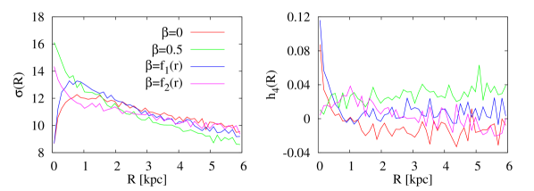
Figure 1: The profiles of the velocity dispersion (left panel) and the 4th Gauss-Hermite moment $h_{4}$ (right panel) for the four haloes with different anisotropy: $\beta=0$ (red), $\beta=0.5$ (green), increasing $\beta$ (blue) and decreasing $\beta$ (magenta).

3 Orbit library

Assuming the density profile matching that of the haloes, we have generated initial conditions for a large library of 5000 representative orbits. The orbits have been integrated using the public $N$-body code GADGET-2 (Springel, 2005) saving in total 2001 points per orbit. Each orbit has been randomly rotated 200 times around two axes of the simulation box and combined. In order to extract the observables, we have projected the stuck orbits along the line of sight and stored them on the same grid as the mock data. The Gauss-Hermite moments have been calculated using formula (7) from van der Marel & Franx (1993) with the values of $\gamma$, $V$ and $\sigma$ the same as fitted to the data.

4 Fitting and results

We find the best-fitting model by minimizing the $\chi^{2}$ function over the weights of the orbits $\gamma_{k}$, following Rix et al. (1997) and Valluri et al. (2004). We used the projected mass, analytically calculated deprojected mass and the Gauss-Hermite moments 0-4. The errors adopted for each quantity are arbitrarily set to $1\%$ for both masses and $0.01$ for Gauss-Hermite moments.

Similarly to fitted observables, we derive the intrinsic velocity dispersions as sums over the orbit library weighted with the deprojected masses. We plot the dispersions in terms of the anisotropy parameter $\beta$ in Fig. 2. We can see that the fitting allows us to recover the intrinsic anisotropy profiles and distinguish between them.

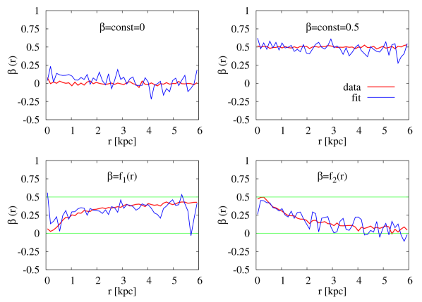
Figure 2: The profiles of the anisotropy parameter for the four haloes: from the mock data (red) and obtained from the fit, i.e. as a result of the Schwarzschild modelling (blue). The asymptotes of the varying $\beta$ profiles are marked in green.

5 Summary

Using numerical realizations of dark matter haloes we have tested the reliability of the Schwarzschild modelling method in recovering the intrinsic anisotropy of orbits. We have fitted a library of orbits to the mock data extracted from four haloes of the same mass distribution but different orbital structure. We have shown that as long as we know the density profile and have a large sample of tracing particles, by fitting just the projected observables we are able to recover with high precision the internal orbital properties of the haloes. In our future work we will extend the application of the method to less idealized conditions.