Pan-Planets: Searching for hot Jupiters around cool dwarfs

The Pan-Planets survey observed an area of 42 sq deg. in the galactic disk for about 165 hours. The main scientific goal of the project is the detection of transiting planets around M dwarfs. We establish an efficient procedure for determining the stellar parameters $\mathrm{T_{eff}}$ and log $g$ of all sources using a method based on SED fitting, utilizing a three-dimensional dust map and proper motion information. In this way we identify more than 60 000 M dwarfs, which is by far the largest sample of low-mass stars observed in a transit survey to date. We present several planet candidates around M dwarfs and hotter stars that are currently being followed up. Using Monte-Carlo simulations we calculate the detection efficiency of the Pan-Planets survey for different stellar and planetary populations. We expect to find $3.0^{+3.3}_{-1.6}$ hot Jupiters around F, G, and K dwarfs with periods lower than 10 days based on the planet occurrence rates derived in previous surveys. For M dwarfs, the percentage of stars with a hot Jupiter is under debate. Theoretical models expect a lower occurrence rate than for larger main sequence stars. However, radial velocity surveys find upper limits of about 1% due to their small sample, while the Kepler survey finds a occurrence rate that we estimate to be at least $0.17(^{+0.67}_{-0.04})$%, making it even higher than the determined fraction from OGLE-III for F, G and K stellar types, $0.14(^{+0.15}_{-0.076})\%$. With the large sample size of Pan-Planets, we are able to determine an occurrence rate of $0.11(^{+0.37}_{-0.02})$% in case one of our candidates turns out to be a real detection. If, however, none of our candidates turn out to be true planets, we are able to put an upper limit of 0.34% with a 95% confidence on the hot Jupiter occurrence rate of M dwarfs. This limit is a significant improvement over previous estimates where the lowest limit published so far is 1.1% found in the WFCAM Transit Survey. Therefore we cannot yet confirm the theoretical prediction of a lower occurrence rate for cool stars.

1 INTRODUCTION

As of July 2015, more than 1900 exoplanets have been discovered, the majority of them with the transit method. One of the most noteworthy discoveries, first detected with the radial velocity method, is the existence of hot Jupiters and hot Neptunes which orbit closely around their host star. Such close-in gas giants were unexpected since there is no equivalent in our solar system. Those planetary systems are of significant interest, not only for their unforeseen existence but also because they are the candidates best-suited for a planetary follow-up study with transit spectroscopy. Their large size lowers the difference between planetary and stellar radius. Besides the dependence on the atmospheric thickness, larger planetary radii improve the S/N of the transmission spectrum by increasing the overall surface area. The radius ratio of hot Jupiters and M-type dwarf stars is particularly favorable, although only very few such systems have been detected so far (Johnson et al., 2012; Hartman et al., 2014; Triaud et al., 2013). It is possible that they are rarer than hot Jupiters around FGK stars since the amount of building material for planets is lower in M dwarf systems (Ida & Lin, 2005; Johnson et al., 2010; Mordasini et al., 2012). Additionally, there is a correlation between metallicity and giant planet occurrence rates for FGK stars (Gonzalez, 1997; Santos et al., 2001; Fischer & Valenti, 2005) with indications for the same correlation for M dwarfs (Johnson & Apps, 2009; Neves et al., 2013; Montet et al., 2014). However, there is still an ongoing discussion about the strength of the metallicity dependence for M dwarfs (Mann et al., 2013; Gaidos & Mann, 2014).
Radial velocity (RV) surveys (Johnson et al., 2007; Bonfils et al., 2013) set an upper limit for the occurrence rate of hot Jupiters around M dwarfs of 1%, however, with no precise estimates due to a small sample of a few hundred target stars per survey. These low sample sizes negate high detection efficiencies.
Transit surveys, such as Kepler (Mann et al., 2012; Dressing & Charbonneau, 2013; Gaidos & Mann, 2014; Morton & Swift, 2014; Dressing & Charbonneau, 2015) and the WFCAM Transit Survey (WTS) (Kovács et al., 2013; Zendejas Dominguez et al., 2013), point to a fraction of less than 1% of M dwarfs that are being accompanied by a hot Jupiter. So far there have been few detections of such M-dwarf hot Jupiters (Johnson et al., 2012; Hartman et al., 2014; Triaud et al., 2013). However, the sample sizes were not high enough to assess the occurrence rate accurately and all detected planets orbit only early M dwarfs.
Since radial velocity surveys provide information about the planetary mass and transit surveys about radii, it is not trivial to compare these results directly. Furthermore, many RV surveys focus on metal-rich host stars which seem to have a higher rate of hot Jupiters (Dawson & Murray-Clay, 2013).
With Pan-Planets, we aim to address this issue by providing a substantially larger sample size. This survey has been made possible by the construction of a wide-field, high-resolution telescope, namely Pan-STARRS1 (PS1).
Pan-STARRS, the Panoramic Survey Telescope and Rapid Response System, is a project with focus on surveying and identifying moving celestial bodies, e.g. Near-Earth Objects that might collide with our planet. The Pan-STARRS1 (PS1) telescope (Kaiser et al., 2002; Hodapp et al., 2004) is equipped with the 1.4 Gigapixel Camera (GPC1), one of the largest cameras ever built. The size of the focal plane is 40 cm $\times$ 40 cm which maps onto a 7 square field of view (Tonry & Pan-STARRS Team, 2005; Tonry & Onaka, 2009). The focal plane is constituted of 60 CCDs which are further segmented into 8 $\times$ 8 sub-cells with an individual resolution of ~600 $\times$ 600 pixels at a scale of 0.258 arcsec per pixel. A complete overview of the properties of the GPC1 camera can be found in table 1. The PS1 telescope is located at the Haleakala Observatory on Maui, Hawaii. The central project of PS1 is an all-sky survey that observes the whole accessible sky area of $3\pi$.
A science consortium of institutes in the USA, Germany, the UK and Taiwan defined 12 key projects in order to make use of the large amount of data being collected by the PS1 telescope. One of these key projects is the dedicated Pan-Planets survey which has been granted 4% of the total PS1 observing time. It began its science mission in May 2010.
With about 60000 M dwarfs in an effective FOV of 42 sq. deg., Pan-Planets is about ten times larger than previous surveys. In a sensitivity analysis of the project using Monte-Carlo simulations (Koppenhoefer et al., 2009), it was estimated that Pan-Planets would be able to detect up to dozens of Jovian planets that are transiting main sequence stars, depending on the observing time and noise characteristics of the telescope. The number of hot Jupiter detections around M dwarfs was undetermined since there was no reliable planetary occurrence rate. The actual photometric accuracy is lower than expected (see following Sect.) but good enough to detect transiting hot Jupiters around K and M dwarfs.
In Sect. 2 we describe the Pan-Planets survey and the data reduction pipeline in detail. Our stellar classification and M dwarf selection is presented in Sect. 3. We detail our transit injection simulation pipeline that is being used for improved selection criteria and determination of the detection efficiency in Sect. 4. An overview of the current survey status is given in Sect. 5. We detail the detection efficiency of the Pan-Planets survey and discuss the results and implications in Sect. 6. Lastly, we draw our conclusions in Sect. 7.

2 SURVEY AND DATA REDUCTION

2.1 Survey setup and execution

GPC specifications
Telescope	1.8m Pan-STARRS1
Camera FOV	7 sq. deg.
Filters	g’, r’, i’, z’, y’
Camera Properties	8x8 CCDs
CCD Properties	8x8 cells with ~600x600 pixels
Pixel scale	0.258 arcsec/pixel
Pan-Planets characteristics
Observation period	May 2010 - Sep. 2012
Observation time	165 hours
Survey FOV	42 sq. deg.
Survey area	301.7∘ ¿ RA ¿ 293.7∘
	21∘ ¿ DEC ¿ 13∘
Exposure time	15 or 30 s
	seeing-dependent
Median FWHM	1.07 arcsec
Photometric band	i’
#target stars	~4 $\mathrm{\cdot 10^{6}}$
Target brightness	13.5 mag $\leq$ i’ $\leq$ 18 mag
M dwarf targets	~60000
White dwarf targets	~4000
Observation time per night	1 or 3 h
Photometric precision	5-15 mmag

Table 1: Properties of the GPC and the Pan-Planets survey.

In 2010, Pan-Planets observed three slightly overlapping fields in the direction of the Galactic plane. In the years 2011 and 2012, four fields were added to increase the total survey area to 42 square degrees in order to maximize the detection efficiency (Koppenhoefer et al., 2009). Fig. 1 shows the position of the seven Pan-Planets fields on the sky in relation to the extragalactic dustmap of Schlegel et al. (1998).

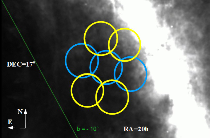
Figure 1: Position of the Pan-Planets fields (coordinates in J2000). The yellow circles correspond to the four fields with data taken only in 2011 and 2012. The blue circles correspond to the three fields with additional data taken in 2010. The background image is an extragalactic dust map taken from Schlegel et al. (1998).

Depending on atmospheric conditions, the exposure time was 30 s or 15 s. Observations were scheduled in 1h blocks. Over the three years of the project, we acquired 165 h of observations, not including 15 h from the commissioning phase in 2009. The target magnitude range of the survey is between 13.5 and 16.0 mag in the i’-band which is expanded down to i’=18.0 mag for M dwarfs. The i’ band is ideally suited for a survey of cool stars, since those are relatively bright in the infrared. Each field is split into 60 slightly overlapping sub-fields (called skycells). The survey characteristics of Pan-Planets are summarized in table 1. More information about the planning of the survey can be found in Koppenhoefer et al. (2009).
Focusing on stars smaller than the Sun has several advantages for the search for transiting planets. The most significant one is that the transit depth, which is the decrease in flux created by the planetary transit, is determined by the square of the ratio between the planetary and stellar radius. The smaller the star, the easier it is to detect the signal since the light drop increases. This makes it possible to search for hot Jupiters around very faint M dwarfs. Moreover, the M-dwarf stellar type is the most abundant in our galaxy, meaning that there is a high number of nearby cool dwarf stars, albeit very faint (Henry et al., 2006; Winters et al., 2015). We estimate that our sample contains up to 60000 M dwarfs (details on our stellar classification can be found in Sect. 3). This M dwarf sample is several times larger than in other transit surveys such as Kepler or WTS, enabling us to determine the fraction of hot Jupiters around M dwarfs more precisely. We show the brightness distribution of our selected M dwarf targets in Fig. 2.

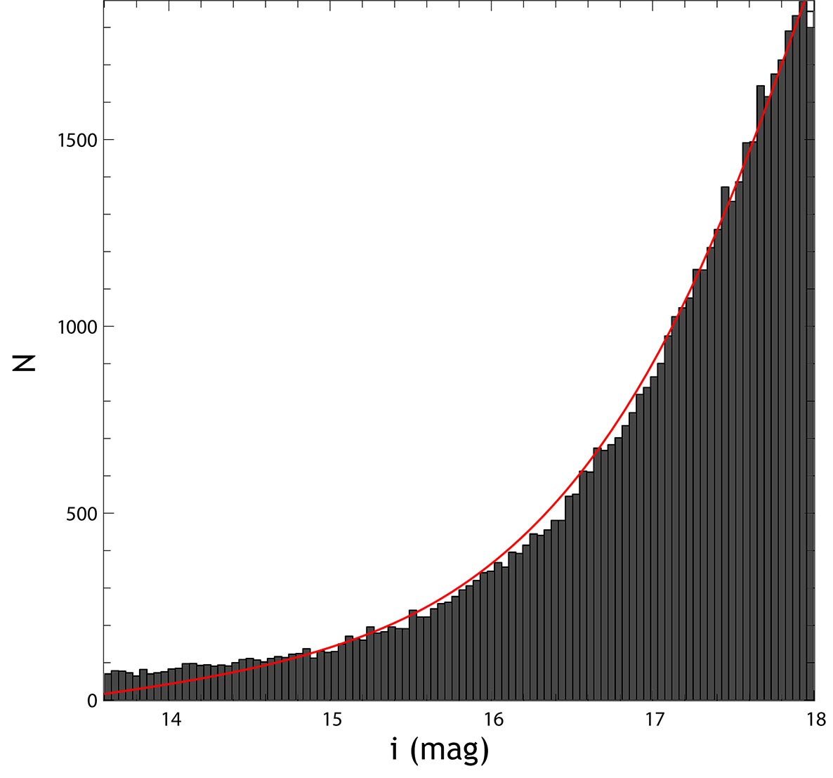
Figure 2: Histogram with 100 bins of the brightness distribution in our M dwarf sample. The red line shows the distribution according to the Besançon model (Robin et al., 2003). Our fields include more bright stars than predicted by the Besançon model, but the number of stars is in good agreement for stars with magnitudes $\mathrm{i^{\prime}\geq 14.5\,mag}$. We further detail our stellar classification method in Sect. 3.

2.2 Basic image processing

All images have been processed in Hawaii by the PS1 Image Processing Pipeline (IPP, Magnier (2006)), which applies standard image processing steps such as de-biasing, flat-fielding and astrometric calibration. Each exposure is resampled into 60 slightly overlapping sub-cells (skycells). Every skycell has a size of $\sim$6000 $\times$ 6000 pixels and covers an area of 30 $\times$ 30 arcminutes on the sky.
During the analysis of the early data releases we realized that several cells of the GPC1 CCDs (mostly located in the outer areas) exhibit a high level of systematics. To account for that, we use time-dependent static masks that we created and provided to the IPP team (see Fig. 3 for the chip mask used for the 2012 data).

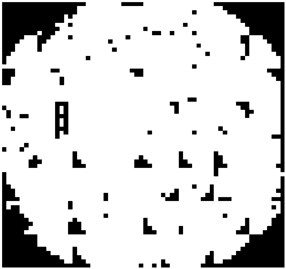
Figure 3: Statically masked areas in the GPC1 camera for the 2012 data. Note that the corners are not illuminated due to the circular layout of the GPC1 camera.

The re-sampled IPP output images have been transferred to Germany and stored on disk for a further dedicated analysis within the Astro-WISE environment (Begeman et al., 2013). During the ingestion of the data into Astro-WISE we correct for several systematic effects. We apply an automated algorithm that searches for and subsequently masks areas that display a systematic offset with respect to the surrounding areas (e.g. unmasked ghosts, sky background uniformities, etc.). Since satellite trails are not removed by the IPP, we apply a masking procedure based on a Hough transformation (Duda & Hart, 1972) that is available in Astro-WISE. Fig. 4 shows an example image before and after the satellite trail masking.

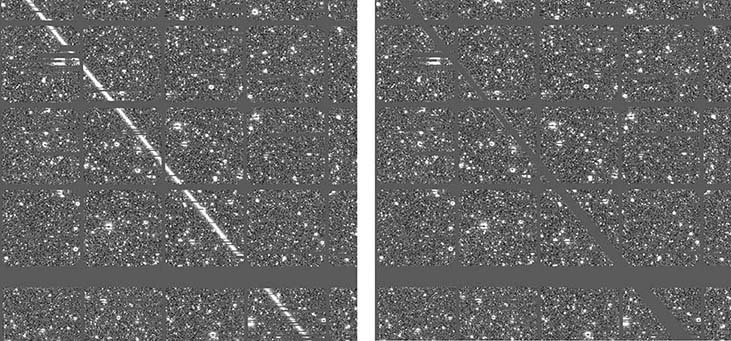
Figure 4: Left: Satellite trail in one of the Pan-Planets images. Right: Result after automatic masking.

Blooming of very bright stars is confined to one of the 8 $\times$ 8 cells of each chip. We apply an algorithm that detects saturated or overexposed areas and then masks the surrounding region, as demonstrated in Fig. 5.

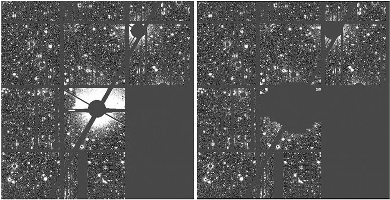
Figure 5: Left: Saturated area that has not been sufficiently masked. Right: Result after application of the automatic masking.

Since the skycells are overlapping and three of the seven field have been observed longer, the total number of frames per skycell is varying between 1700 and 8400. Fig. 6 shows a histogram of the number of frames per skycell.

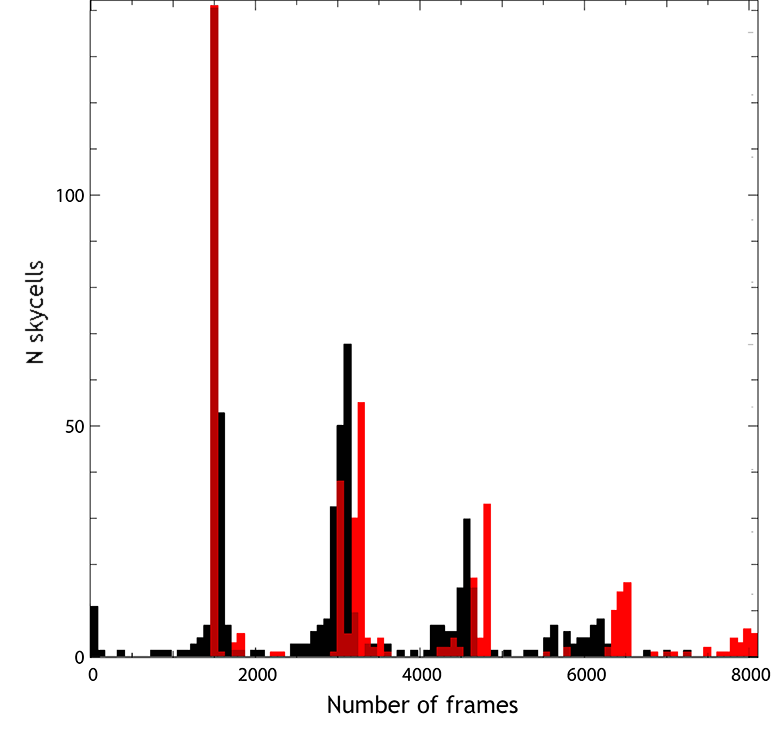
Figure 6: Histogram of the number of frames per skycell, of which there are 420 overall. In red we show the distribution per skycell before ingesting the images into the pipeline, in black after ingesting. One can see that the smallest overlapping region completely vanishes and only a small fraction of skycells with about 6000 frames remains.

Within one skycell there is significant masking in a majority of the frames. Our data reduction pipeline discards any frame with less than 2000 visible sources, which corresponds to masking of about 85%. The histogram of remaining frames is shown in Fig. 6 in black. One can see that many images from the overlapping regions with a high initial number of images (red) are dropped due to high masking. The comparatively low resulting number of frames, especially in the four less visited fields, significantly influences the detection efficiency for planets with long periods or shallow transits.
There is a noticeable difference in data quality between the 2010 data in comparison to the 2011 and 2012 data. In the first year, the camera read-out resulted in a systematic astrometric shift of bright sources (i’ $\leq$ 15.5 mag) with respect to faint sources. This effect was noticed in early 2011 and fixed by adjusting the camera voltages. In order to account for the shifted bright stars, we use custom masks in our data analysis pipeline for the 2010 data.

2.3 Light curve creation

The Pan-Planets light curves are created using the Munich Difference Imaging Analysis (MDia) pipeline (Koppenhoefer et al., 2013; Gössl & Riffeser, 2002). This Astro-WISE package makes use of the image subtraction method which was developed by Tomaney & Crotts (1996) and later by Alard & Lupton (1998). The method relies on the creation of a reference image, which is a combination of several images with high image quality, i.e. very good seeing and low masking. As discussed in Koppenhoefer et al. (2013), increasing the number of input images increases the S/N of the reference frame. However, each additional image broadens the PSF which means that resolution decreases. Due to the high masking in the Pan-Planets images (the average masking is $\sim$40% including cell gaps) we decide to use a high number of 100 input images, resulting in a typical median PSF FWHM of 0.7 arcseconds in the reference frame.
The procedure to select the 100 best images is the following: after removing all frames with a masking higher than 50%, we select the 120 images with the best seeing. We determine the weight of each image on the reference frame by determining the PSF FWHM and S/N and reject frames that possess a very low weight (less than half of the median weight) or too high weight (higher than twice the median weight), which usually results in 10 removed frames. This is necessary in order to avoid using bad images that do not contribute in S/N or images that would dominate the final reference frame, adding noise. Out of the remaining images we clip the frames with the broadest PSF until we have the final list for the best 100 frames. These images are subject to a visual inspection in which any leftover systematic effect is masked by hand before combining the images to create the reference frame.
The next step is to generate the light curves for each individual source. We photometrically align each image to the reference frame and correct for background and zeropoint differences. Subsequently we convolve the reference image with a normalized kernel to match the PSF of the single image and subtract it. In the resulting difference image we perform PSF-photometry at each source position. We calculate the total fluxes by adding the flux measured in the difference images with the flux in the reference image which is measured using an iterative PSF-fitting procedure. Fig. 7 shows a histogram of the number of datapoints for each source. One can see two broad peaks. The second peak, having more data points, is created by the additional observations for 3 fields that were taken in 2010.
Since the output light curves of MDia are at an arbitrary flux level, we calibrate them by applying a constant zero point correction for each skycell that is derived using the 3$\pi$ catalogue (version PV3) from Pan-STARRS1 as a reference.

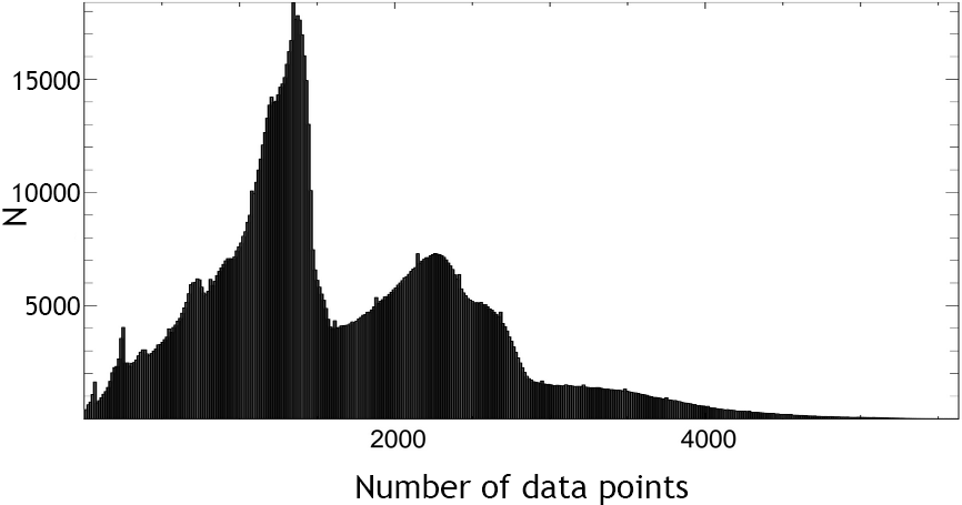
Figure 7: Histogram of the number of data points per source. One can see two larger peaks, being created by the additional observations for 3 fields in 2010. Overlapping regions, seeing-dependent exposure times and static masking of some detector areas broaden those peaks. The additional data from overlap further create a tail, reaching up to 5000 data points.

While analysing the light curves, we found that some data have a lower quality depending on the time of observing. This applies mostly to the 2009 data for which a different camera configuration and survey strategy were used. Hence, we decide to disregard the 2009 data for the further data reduction. We perform an a-posteriori error bar correction on the light curves. This is done by rescaling the error values of every light curve using a magnitude-dependent scaling factor, derived by fitting a forth-order polynomial to the magnitude dependent ratio between the median error value and the RMS of each light curve.
To remove systematic effects that appear in many light curves, we apply the sysrem algorithm that was developed by Tamuz et al. (2005). The concept of sysrem is to analyse a large part of the data set, in our case one skycell, and identify systematic effects that affect many stars at the same time. The strength of this algorithm is the fact that it does not need to know the cause of the systematic effects it corrects. However, for sysrem to work properly, we have to remove stars with high intrinsic variability from the data sample beforehand. We do this by eliminating stars which have a reduced $\chi^{2}$ higher than 1.5 for a constant baseline fit which subsequently also do not get corrected by $sysrem$. This way, we include about 80% of the light curves. Fig. 8 shows the overall quality of the light curves and the improvement that is achieved by utilizing this algorithm, namely the $RMS$ scatter of the Pan-Planets light curves as a function of i-band magnitude. At the bright end we achieve a precision of $\sim$5 mmag.

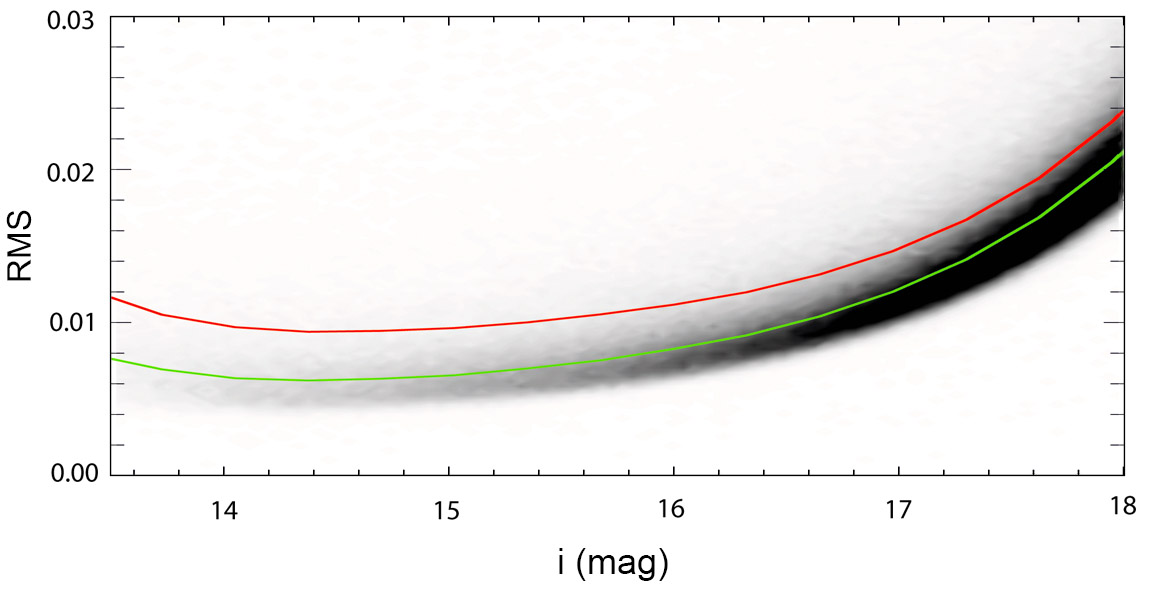
Figure 8: Density plot of $RMS$ against the i-band magnitude in the central field after iterative clipping of 5$\sigma$ outliers and application of the sysrem algorithm. The green line shows the median values in 0.2 mag bins, the red line the values before application of sysrem. Note that the phase is shifted by 0.5 units for better readability.

2.4 Light curve analysis

We search for periodic signals in the Pan-Planets light curves with an algorithm that is based on the box-fitting least squares (BLS) algorithm of Kovács et al. (2002). It is very efficient in detecting periodical signals which can be approximated by a two level system, such as a planetary transit. We extend the BLS algorithm by a trapezoid-shaped re-fitting at the detected periods, which we call transit v-shape fitting. A value of 0 corresponds to a box shape and 1 to a V. It is a better representation of the true shape of eclipse events. Further, we fit for a possible secondary transit, offset by 0.5 phase units, in order to discriminate between planets and eclipsing binaries. Eccentric orbits are not uncommon for binaries, hence the secondary might also appear at different phases. Our BLS algorithm is not optimized to detect secondary eclipses at phases other than 0.5. Eclipsing binaries of interest (see Sect. 5.2) that exhibit visible eccentricity will be analysed further with an adaptation of our BLS code. More detailed information on the modifications of our BLS algorithm can be found in Zendejas Dominguez et al. (2013).
We test 100001 periods distributed between 0.25 and 10 days for each light curve. In order to speed up the fit we bin the phase folded light curve to 500 points, a number which we determined through dedicated Monte-Carlo simulations (same as in Sect. 4) in which we determined the effect of binning on the detection efficiency. The transit duration is limited to 0.25 phase units. This does not constrain the planet transit duration. As an extreme case. the duration for a hot Jupiter with a 12 h period around an M5 dwarf would still be less than 0.05. For non-circular orbits, the duration can increase, however, hot Jupiters are generally on rather circular orbits. The highest transit duration in our candidate sample is about 0.07. A typical plot of our signal detection output is shown in Fig. 9.

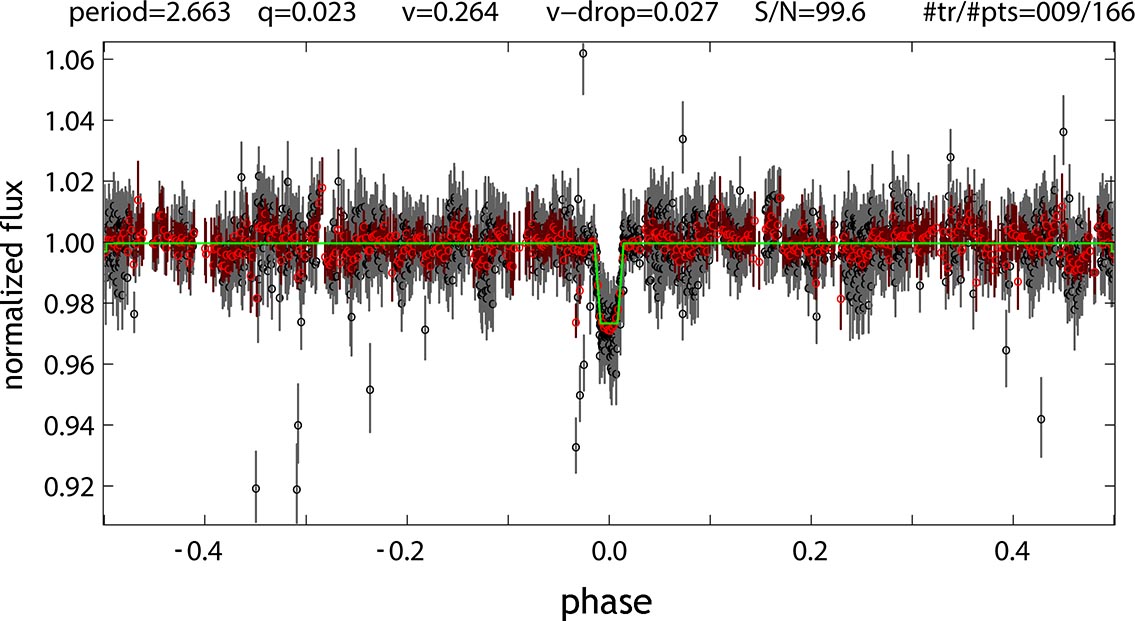
Figure 9: Typical plot of our signal detection algorithm for object 1.40_14711, a K dwarf being orbited by a hot Jupiter candidate. Low resolution spectroscopy confirms the stellar type determined through SED fitting (see also Sect. 3). Shown at the top are period (days), transit duration q (in units of phase), transit v shape (0 corresponds to a box, 1 to a V), transit light drop, S/N and number of transits/number of points in the transits. The binned data points are shown in red. A green line shows the best-fitting 2-level system, including the v-shape adjustment.

2.5 Transit recovery

Having completed the BLS run, we need to preselect the light curves with a possible signal before visual inspection due to our large sample. We retain the four best BLS detection for each light curve, i.e. those having the highest S/N. We remove results close to alias periods introduced by the window function of the observing strategy by utilizing Monte-Carlo simulations (see Sect. 4). Out of the remaining detections we select the best fit, i.e. the one with the lowest $\chi^{2}$ of the trapezoidal re-fit.

3 M DWARF SELECTION

The large amount of M dwarfs in our sample makes it unfeasible to perform a spectroscopic characterization for every star. Instead, we utilize a combination of photometric and proper motion selection criteria. Strong reddening in several of our fields is problematic when using colour cuts. Distant giant stars can be misclassified as M dwarfs as well as hotter main sequence stars that appear cooler due to reddening. This kind of misclassification could lead to large uncertainties in our sample. We therefore utilize the Spectral Energy Distribution (SED) fitting method which allows us to estimate the effective temperature of stars through fitting of synthetic SEDs to multi-band photometry and identify the best-fitting model for every star. We limit the issue of dust reddening by making use of a distance-dependent dustmap (see following Sect.).

3.1 SED fitting

A necessary assumption for SED fitting is that the model stars are physically accurate since any issue in the synthetic sample has a strong impact on the selection process. We use four synthetic stellar libraries for the fit. The first one is the Dartmouth isochrone model from Dotter et al. (2008). This database provides values for stellar mass, luminosity, surface gravity, metallicity and effective temperature. We limit the grid to solar metallicity since we encountered similar issues as Dressing & Charbonneau (2013), getting an overabundance of high-metallicity results. Furthermore, we use the PARSEC stellar isochrones (Bressan et al., 2012) which are based on the Padova and Trieste stellar evolution code. We choose the newest version that is improved for low-mass stars (Chen et al., 2014). In order to achieve improved results at the lower mass region, we include the most recent isochrones from Baraffe et al. (2015) and the BT-Dusty models (Allard et al., 2012). Our final sample contains 25880 model stars with ages of 1-13 Gyr, masses of 0.1-40.5 M_⊙, effective temperatures of 1570-23186 K and radii of 0.13-299.61 $R_{\odot}$.
The fit becomes more precise with a higher amount of photometric information. We use the Pan-STARRS1 $3\pi$ survey (version PV3) bands g’, r’, i’, z’ and the 2MASS bands J, H and K and combine those catalogues by coordinate matching. We decide not to include the PS1 y-band for our fitting process. Conversion into the PS1 photometric system is achieved with polynomial extrapolation of the z magnitude. Therefore, adding the y band would provide no useful physical information for the fit but create a bias towards the z photometry. After merging we achieve completeness for 62% of all stars. For the remaining 38% we only have PS1 photometry. Most of the missing stars are saturated in 2MASS. For stars that are listed in 2MASS, we have full photometric information in all seven bands for the majority of them (94%). We do not impose thresholds on the 2MASS quality flags. In order to stay consistent with our stellar targets, we limit the brightness range to $\mathrm{13.5\,mag\leq i_{PS1}\leq 18\,mag}$ for this catalogue.
Our first step is to determine the best-fitting distance modulus for each isochrone and photometric band $x$. The $\chi^{2}$ value of the distance fit for a star with apparent brightness $m_{x}$, distance modulus $d$ and the absolute brightness $M_{x}$ of the synthetic isochrone star is described by following term:

$$\chi^{2}=\sum\limits_{x}\frac{(M_{x}-m_{x}+d)^{2}}{e_{x}^{2}}.$$ (1)

Here, $e_{x}$ is the error of the magnitude $m_{x}$. We assume no errors for $M_{x}$. In order to find the best-fitting distance, we need to determine the minimum of $\chi^{2}$, therefore we take the derivative, solve it for the distance and end up with:

$$d=\frac{\sum\limits_{x}\frac{m_{x}-M_{x}}{e_{x}^{2}}}{\sum\limits_{x}\frac{1}{e_{x}^{2}}}.$$ (2)

In case of zero extinction, this would give us the best fit for the distance. However, dust reddening is a significant factor for a large part of our fields. In order to solve this problem, we make use of the 3D dust map provided by Green et al. (2015). It gives a statistical estimate for the amount of colour excess E(B-V) for any point in our field, in distance modulus bins of 0.5 mag in the range between 4 mag and 15 mag. We therefore assign a reddening term $\mathrm{R(d)\cdot f_{x}}$ for every star with a given distance modulus d, reddening coefficient $\mathrm{f_{x}}$ and photometric band x. We determine the reddening coefficients for each band through the web service NASA/IPAC Extragalactic Database (NED), substituting the UKIRT J, H and K values for the 2MASS filters, using the dust estimates from Schlafly & Finkbeiner (2011).
Fitting with a step function-like dust distribution results in artefacts. A first-order linear interpolation leads to similar, albeit weaker, artefacts. We therefore smooth by fitting a 10-th order polynomial to the points. This way, the distribution is artefact-free. With the given reddening R(d) for the best-fitting distance modulus d, we iterate the fit until the converging criterion

$$\mathrm{d_{difference}=|d_{n+1}-d_{n}|\leq 10^{-4}}$$ (3)

is fulfilled. This procedure is executed for each isochrone, after which we select the best fit based on the lowest $\chi^{2}$ value. We interpolate missing error values in 2MASS by first fitting a magnitude-dependent polynomial to each band and then assigning the value for the given magnitude. When comparing the $\chi^{2}$ values in relation to the measured distances, we find that there are usually two distinct local minima. This is explained by fitting two different stellar populations, e.g. main-sequence and giant branch. The resulting local minima sometimes show a very similar $\chi^{2}$, which makes it difficult - in those cases - to distinguish between different stellar populations. In order to solve this, we include proper motion information (see following subsection) into the classification.

3.2 Proper motion selection

Proper motion, in short PM, quantifies the angular movement of a star in the course of time from the observer’s point of view. This is strongly correlated with the distance: the closer a star is to the observer, the higher (on average) the angular motion. Therefore we can be confident that if a star exhibits a high proper motion, the fit for the close distance is the most plausible one.
For this we utilize a combination of the USNO-B digitization of photometric plates (Monet et al., 2003), 2MASS (Skrutskie et al., 2006), the WISE All-Sky Survey (Wright et al., 2010) and the 3$\pi$ Pan-STARRS1 survey as described in Deacon et al. (2015). After calculating the annual proper motion, we assign each star a quality flag depending on the properties shown in table 2. We select every cool star with quality flag 1, even if the best fit is slightly in favour of a distant red giant, and cool stars with the best fit for a dwarf type with quality flags 2, 4 and 5.

Quality flag	PM value	Error
1	PM $\geq 6$ $mas/yr$	$PM_{error}/PM\geq 0.5$
2	PM $\geq 6$ $mas/yr$	$PM_{error}/PM<0.5$
3	PM $<6$ $mas/yr$	$PM_{error}/PM\geq 0.5$
4	PM $<6$ $mas/yr$	$PM_{error}/PM<0.5$
5	No coordinate match.

Table 2: Quality flags for different proper motion PM (mas/yr). Stars having flag 3 do not pass our criteria, having no measurable proper motion.

We further use the criterion $\mathrm{J-K>1}$ as a flag to discriminate likely background giants from closer dwarf stars. This has proven to be very effective in the Kepler project (Mann et al., 2012).

3.3 Consistency check with the Besançon model

We compare our results to the Besançon model (Robin et al., 2003) which provides a synthetic stellar population catalogueue for any given point of the sky. We simulate our entire FOV in 1 sq. deg. bins. We use this to estimate the distribution of spectral types in our target brightness. Choosing the criteria of an effective temperature ¡ 3900 K and surface gravity ¿ 4, we identify 62800 M dwarfs in the Besançon model. We select M dwarfs in our survey with the following criteria:

• SED fitting Temperature ¡ 3900 K

• Quality flag of 1 OR
  2, 4, 5 and a best fit for a nearby dwarf star

With those criteria, we select 65258 M dwarfs in our FOV (about 12000 M dwarf per field since there are multiple identifications in the overlapping regions). This is fairly consistent to the number of M dwarfs in the Besançon model, however, our result is slightly higher. It is possible that there are false positive identifications in the selection list, reddened by dust from the galactic disc. This most likely affects identifications without proper motion data, i.e. flags 2, 4 and 5. However, the difference between our selection and the model distribution is not very large, so the amount of contamination is low.

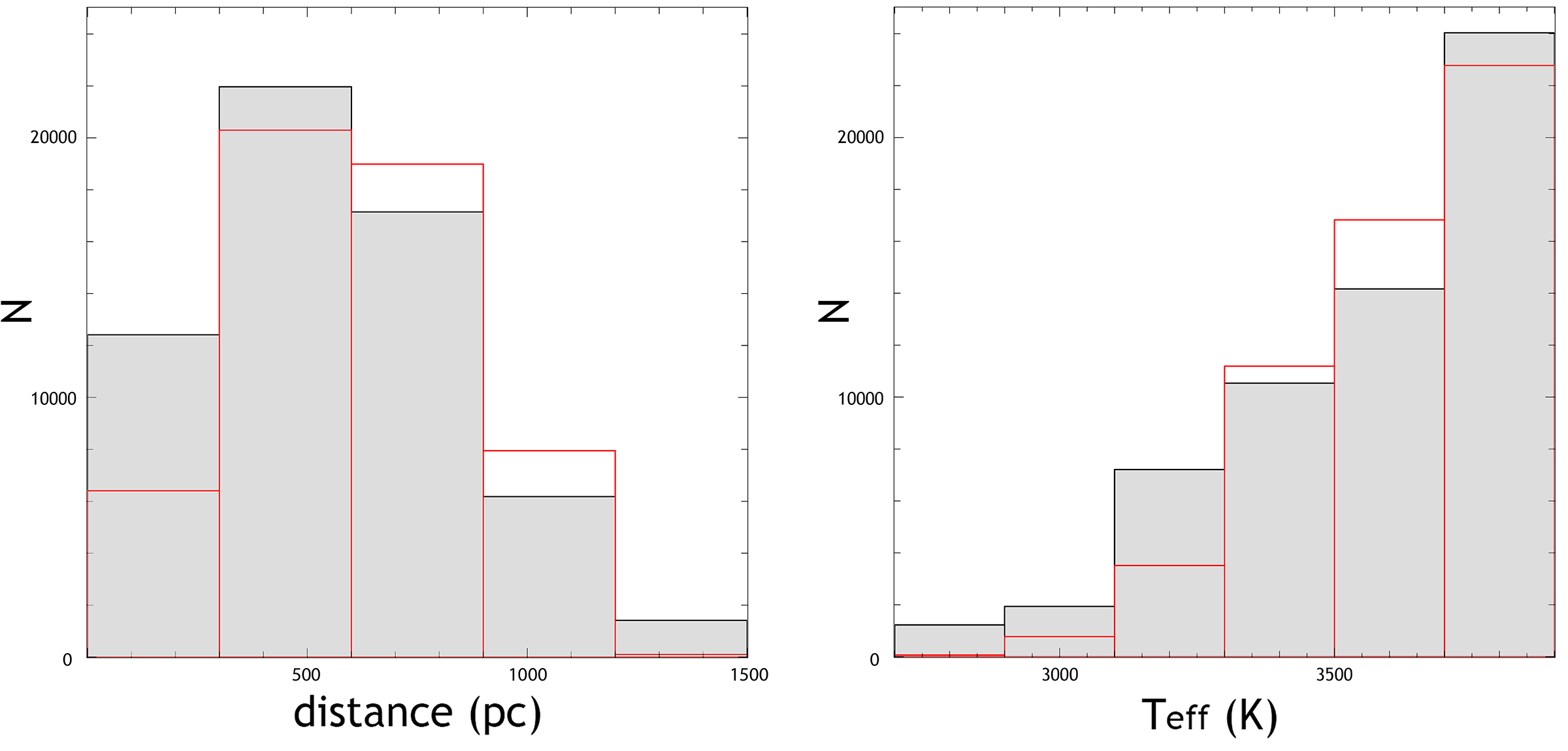
Figure 10: Left: distribution of distances for selected M dwarfs from SED fitting (gray with black bar lines) and the Besançon model (red bar lines). Right: distribution of effective temperatures for selected M dwarfs from SED fitting (gray with black bar lines) with the expected distribution from the Besançon model (red bar lines).

Fig. 10 displays our implemented M dwarf selection and how it compares to the Besançon model. The effective temperatures are fairly consistent, assuming an uncertainty of $\pm$100 K for SED fitting. The distribution of distances does not seem to fit so well as the temperatures, however, we are mainly focused on fitting the effective temperature.

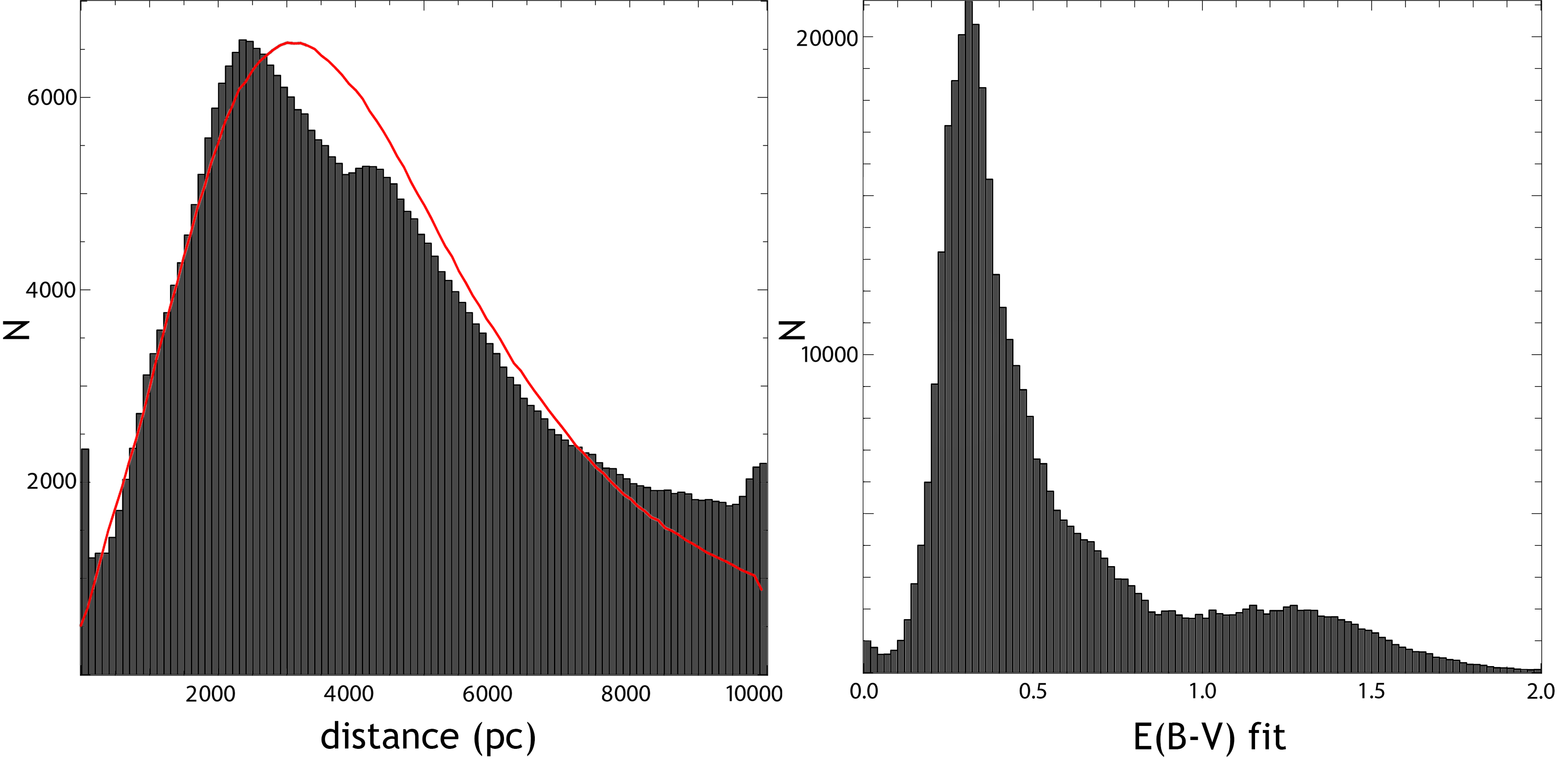
Figure 11: Left: distribution of distances for all fitted stellar types, with the Besançon model as a comparison (red line). Right: distribution of fitted extinction in our field.

Fig. 11 shows the distribution of distances for all fitted stars in comparison to the Besançon model. It seems to be very consistent in closer ranges, both distributions having their peak around 3 kpc, but there are small divergences in the occurrence of distant ($\mathrm{\geq 3\,kpc}$) stars. We are focused on nearby main-sequence stars so this is not much of a concern. In the same Fig. one can see the distribution of fitted extinction E(B-V) which peaks around an E(B-V) value of 0.4.

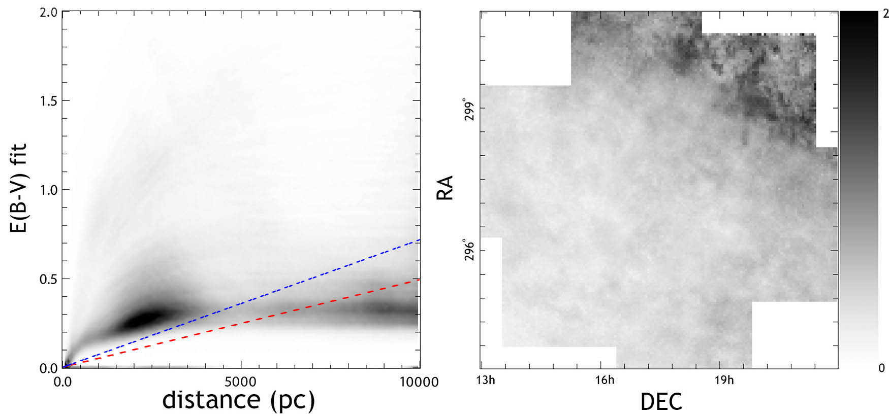
Figure 12: Left: fitted reddening E(B-V) against distance for all fitted stars. As a comparison, linear extinctions of 0.7 mag/kpc (red) and 1 mag/kpc in the V-band as used in the Besançon model and in Dressing & Charbonneau (2013), respectively, are overplotted as dashed lines. Right: average fitted E(B-V) in relation to the coordinates (J2000). One can see the dust-rich region in the upper right which is closer to the galactic disc.

In Fig. 12 on the left is shown the relation between distance and reddening E(B-V) for all fitted stars while the right side of Fig. 12 shows the average reddening in relation to the coordinates. As a comparison, we overplot the linear extinction models of 0.7 mag/kpc as used in the Besançon model (red) and 1 mag/kpc as used in (Dressing & Charbonneau, 2013) (blue). There is a noticeable difference for distances below 3 kpc to our fitting. The outliers with an E(B-V) of more than 1.0 are due to the dust-rich region close to the galactic disc, shown in Fig. 12 on the right (top-right corner).

3.4 Consistency check with Kepler targets

As another consistency check, we take the SED fitting results used for 31 Kepler candidate M-dwarf host stars (Dressing & Charbonneau, 2013), identify the stars in the Pan-STARRS 3$\pi$ catalogue and perform SED fitting. In order to make the process more comparable, we limit our isochrones to less than solar masses, temperatures lower than 7000 K and run the comparison with their model of extinction fitting, i.e. 1 mag in the V-band per kpc.

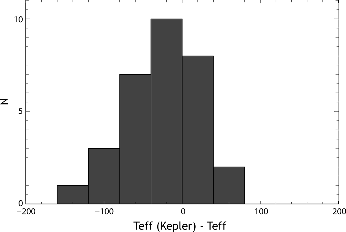
Figure 13: Difference of the calculated effective temperature between our SED fitting results and those of Dressing & Charbonneau (2013).

As one can see in Fig. 13, the results are fairly consistent but at the same time there is a systematic offset of about -25 K. A likely explanation is that the fitting results from Dressing & Charbonneau (2013) are for slightly older and therefore cooler stars. Additionally, the inclusion of non-solar metallicities might also explain or contribute to the shift. However, the difference is not very large. We estimate to have an uncertainty of about $\pm 100\,K$ which is larger than the observed difference.

3.5 Consistency check with spectroscopically confirmed M dwarfs

As the final consistency check, we arbitrarily select 1000 confirmed M dwarfs out of the Sloan Digital Sky Survey Data Release 7 Spectroscopic M Dwarf Catalog (SDSS DR7) (West et al., 2011) that

• exist in the PS1 3$\pi$ catalogue

• exist in the 2MASS catalogue

• have distance-dependent extinction data from Green et al. (2015)

• have data in all 7 bands

• fit our target brightness range (13.5 $\leq$ i’ $\leq$ 18).

This way we can make sure that the comparison is as close as possible as we use our regular stellar characterization pipeline. We find that all of the listed M dwarf candidates are being identified as M dwarfs. Unfortunately, the effective temperatures of the SDSS DR7 catalogue are given in 200 K bins, meaning that there is an inherent error of $\mathrm{\pm 100\,K}$ when comparing their estimates to ours. However, as is shown in Fig. 14, there is very good agreement in the characterized temperatures between both methods.

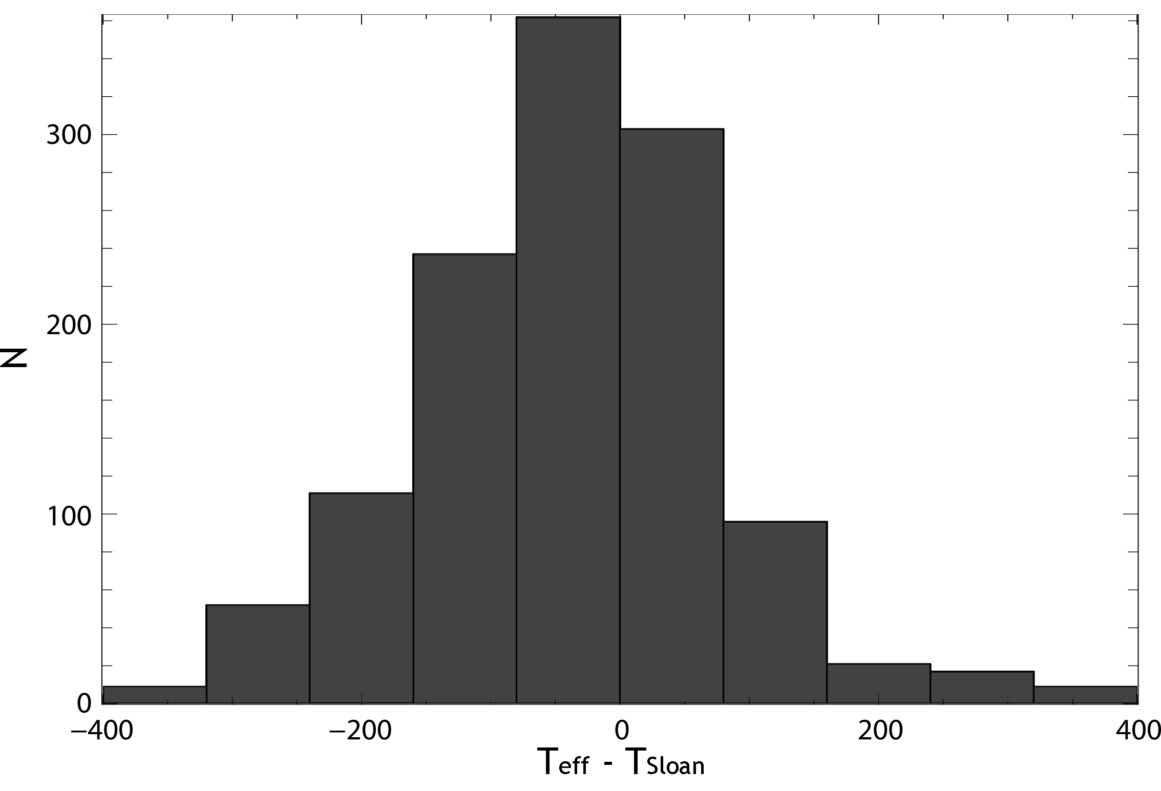
Figure 14: Difference in fitted temperature between SED fitting and spectral fitting of the Sloan catalogue. Note that the temperature estimates from Sloan are in 200 K bins, hence a scatter of $\mathrm{\pm 200\,K}$ is to be expected.

3.6 SED fitting example

To further confirm our SED fitting method, we recorded low resolution spectra for all 18 planet candidate stars with the Otto Struve 2.1m Electronic Spectrograph 2 (ES2) - a low resolution spectrograph. We illustrate the results for SED fitting and spectroscopy for candidate 1.40_14711, a clear example of a late K dwarf. The candidate’s light curve is shown in Fig. 9, in Fig. 15 its spectrum.
With the spectrum we can confirm that the primary in this system is in fact an K dwarf at the boundary to the M dwarf regime, with strong NaD absorption around 5900 Å, broad CaH absorption bands and very weak absorption in the H$\alpha$ band at 6563 Å. The best fit of the surface gravity sensitive Na I doublet (Mann et al., 2012) is shown in Fig. 15 on the left. The best result from spectroscopy is a star with log(g) of 4.5 and an effective temperature of between 4000 K and 4250 K, which is in good agreement with SED fitting. We further used the gravity sensitive region of 6470-6530 Å which are dominated by Ba II, Fe I, Mn I and Ti I lines (Torres-Dodgen & Weaver, 1993).

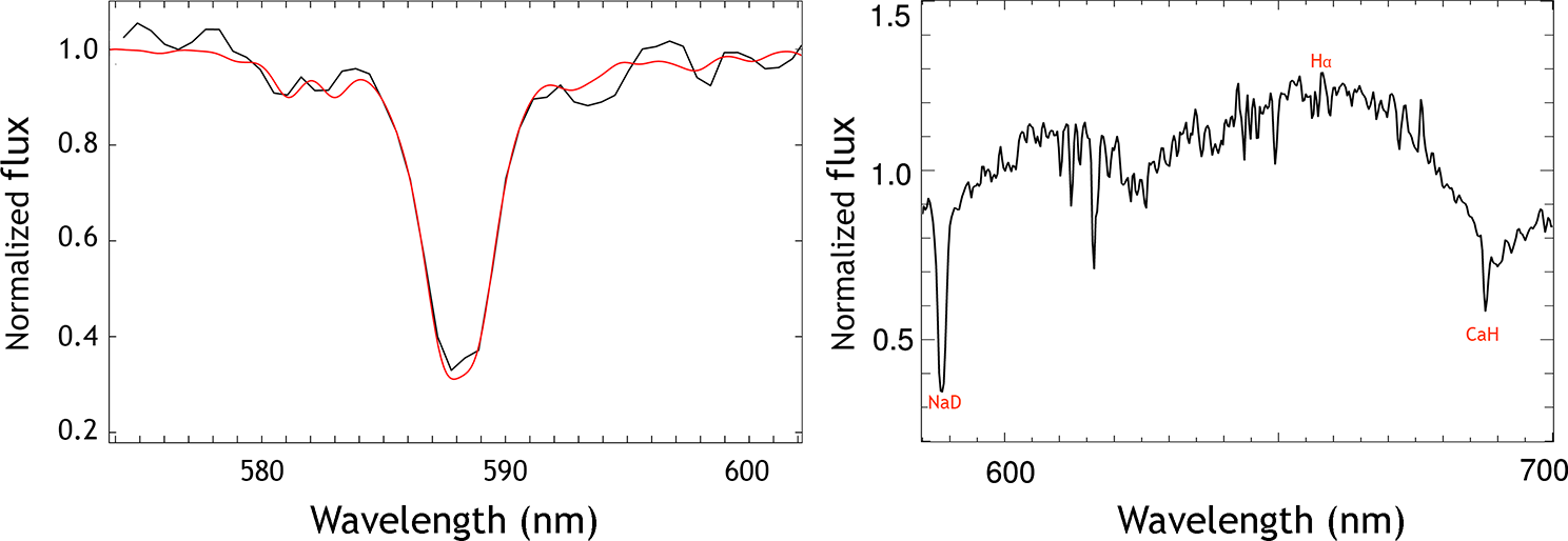
Figure 15: Left: Best spectral fit (red) of the Na I line taken with the Otto Struve 2.1m ES2 low resolution spectrograph (black). Right: Complete spectrum recorded with the ES2 spectrograph with spectral features marked in red.

The SED fitting results for this candidate are shown in Fig. 16, with a best-fitting distance of 293 pc and effective temperature of 4208 K. It is quite obvious that there is no alternative result that would have an equally good fit, e.g. a distant K or G giant reddened by dust. One can also see that our extinction fitting shifts the best-fitting temperature by about 125 K.

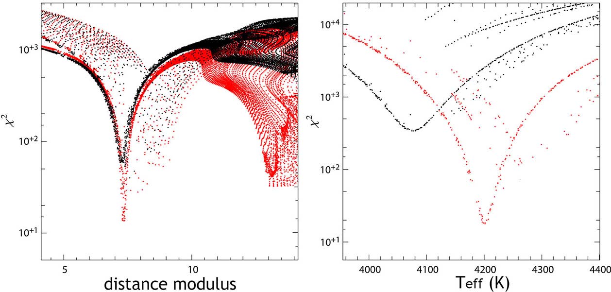
Figure 16: Left: $\chi^{2}$ vs. distance modulus for hot Jupiter candidate system 1.40_14711 with our implemented version of dust fitting (red), compared with a fit without extinction fitting (black). Right: $\chi^{2}$ vs. effective temperature for the same system with (red) and without (black) extinction fitting. It is clear that SED fitting considerably improves $\chi^{2}$ and that there is no other alternative fit with an equally good fit.

4 TRANSIT INJECTION SIMULATIONS

The primary purpose of Pan-Planets is the detection of transiting hot Jupiters while setting new boundaries for the occurrence rate of close-up Jovian planets around M dwarfs. In order to do that, we need to determine the detection efficiency of this project. We perform extensive Monte-Carlo simulations, injecting planetary transit signals into the Pan-Planets light curves and trying to recover the signal. This is similar to other recent approaches performed on Kepler data, e.g. in Petigura et al. (2013a, b), Christiansen et al. (2015) or Dressing & Charbonneau (2015). However, we utilize our full signal detection pipeline instead of inferring successful detections from calculating the number of visible transits combined with noise and signal to noise estimates. Our approach is much more suited to the peculiarities of Pan-Planets. A varying amount of data points, strong constraints for observational window functions and not well-defined systematics mean that this is the only reliable way of estimating our detection efficiency.

4.1 Setup

We start by selecting all previously identified M dwarf light curves minus the identified planetary candidates. We create a simulated distribution of different stellar parameters based on the Besançon model (Robin et al., 2003) for our FOV. Each model star is assigned a set of real light curves, based on brightness. The whole process is illustrated in Fig. 17.

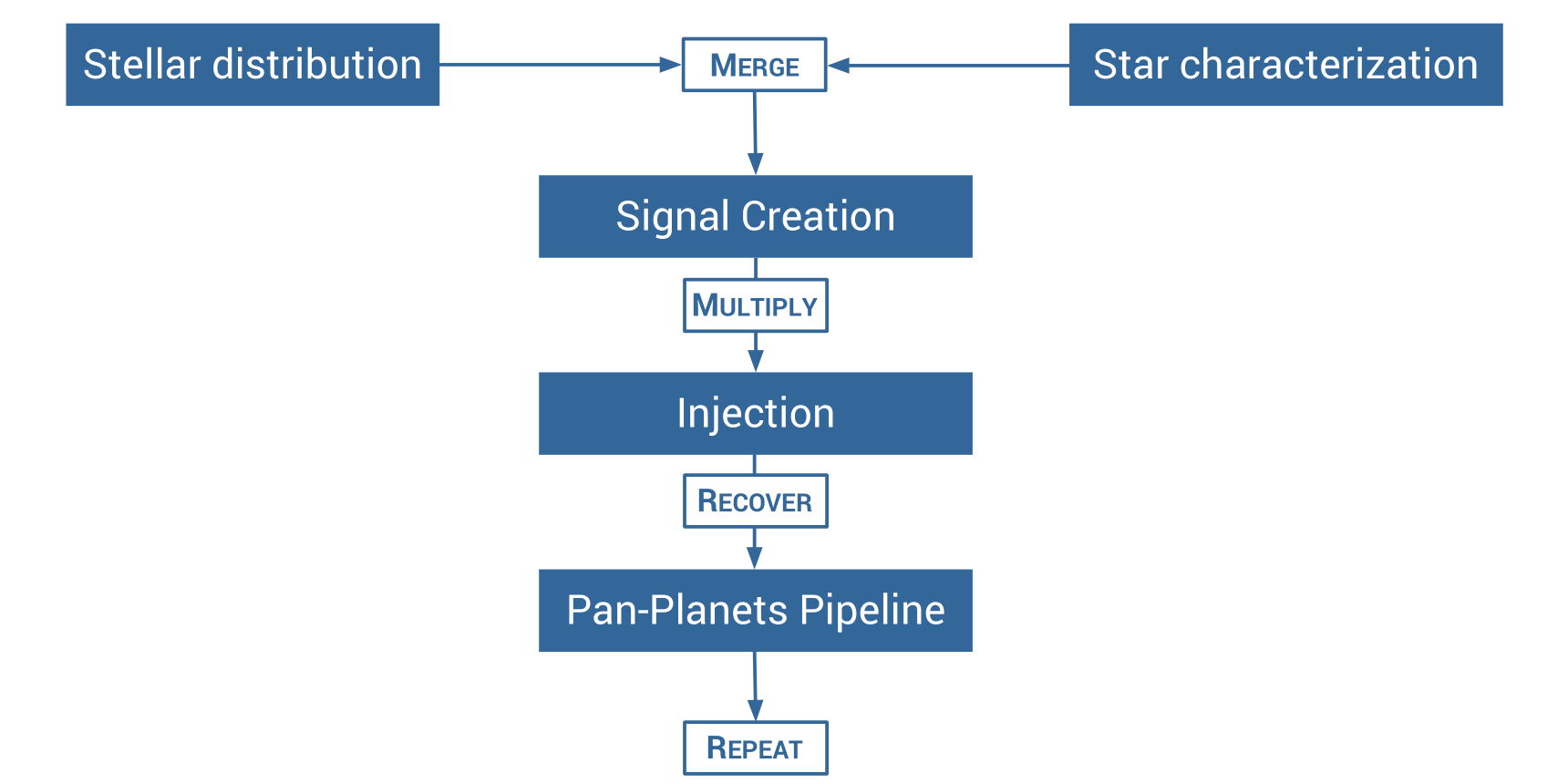
Figure 17: Illustration of our simulation process. We take the model stellar distribution and assign each of our characterized star to the closest-fitting model. We create a planetary signal out of the given stellar and planetary parameters, multiply it with the light curve and try to recover the injected transit with our Pan-Planets pipeline.

In the next step, we create our target planet population by setting up random distributions of period and radius in defined boundaries. In accordance with Hartman et al. (2009), Koppenhoefer et al. (2009) and Zendejas Dominguez et al. (2013), we use five different populations: Jovian planets with radii 1.0-1.2 R_J and periods of 1-3 days, 3-5 days and 5-10 days plus Saturn-sized and Neptune-sized populations with periods of 1-3 days and radii of 0.6-0.8 R_J and 0.3-0.4 R_J, respectively.
We then take every star in the stellar distribution, randomly pick one of the corresponding light curves and select an arbitrary planet out of the chosen population. We assign a random geometrical inclination of the planetary orbit to each star and calculate the criterion

$$sin(i)<\frac{R_{star}+R_{planet}}{a},$$ (4)

where $i$ is the inclination and $a$ the distance to the star. For simplicity, we assume a circular orbit. If this criterion is met, we create a transit signal based on all given parameters, i.e. planetary and stellar radii, inclination, period, t₀ and corresponding limb darkening coefficients (Claret & Bloemen, 2011) for the stellar type. We multiply the simulated signal with the real light data and end up with simulated light curve that possesses all the characteristics of our survey, e.g. noise, systematics, distribution and amount of data points. Further information about the transit injection method used can be found in Koppenhoefer et al. (2009).

4.2 Transit recovery

As the next step we attempt to recover the simulated signals with our transit detection pipeline. As for the survey, we select the 4 best periods with highest S/N for every source. We remove results close to alias periods introduced by the window function of the observing strategy (see table 3).

Excluded alias periods
0.315-0.335 days
0.498-0.500 days
0.991-1.004 days
1.586-1.594 days
1.594-1.600 days
1.965-1.975 days
2.039-2.045 days
2.359-2.360 days
3.370-3.378 days
4.022-4.030 days
4.078-4.088 days

Table 3: List of excluded alias periods that are common for false detections. We identified those periods as peaks in the abs(p_sim-p_det)/p_sim histogram.

Most alias cuts are not directly around harmonics of 1 day but instead slightly lower periods due the observation characteristic of seasonal change and large time gaps. Fig. 18 shows the cut that we used for the alias period of 1 day.

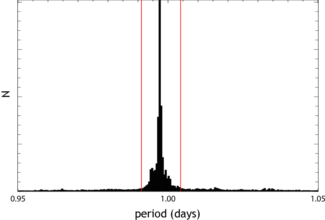
Figure 18: Alias period around 1 day for an arbitrary number of hot Jupiter simulation runs, comprising the whole simulated period range of 1 to 10 days. The red lines mark the excluded period range from table 3. Due to window functions of the survey, the peak is not directly at period 1.0 days, but slightly shifted to the left.

Out of the remaining folded light curves we keep the one with the best $\chi^{2}$ fit. In order to examine whether we could successfully recover the signal, we compare the detected period $p_{det}$ to the simulated period $p_{sim}$. This is the most reliable way of judging whether the detection was successful or not and has been utilized by other surveys as well (Kovács et al. (2013), Zendejas Dominguez et al. (2013)). The low number of data points in some light curves makes the false detection of an harmonic of the period not unlikely. We accept a period deviation of 0.02%, as shown in Fig. 19, and harmonics of $p_{sim}$ with orders of 0.5, 2 and 3 and following period deviations:

$$\frac{p_{sim}}{p_{det}}=0.5\pm 0.0001.$$ (5)

$$\frac{p_{sim}}{p_{det}}=2\pm 0.0001,$$ (6)

$$\frac{p_{sim}}{p_{det}}=3\pm 0.00015,$$ (7)

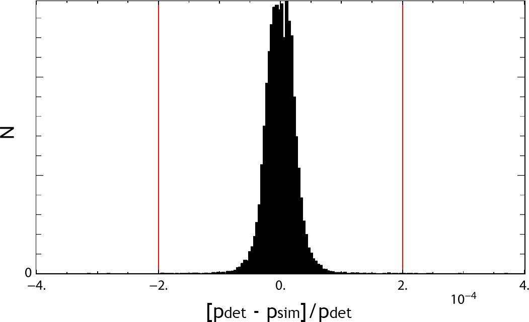
Figure 19: Deviation of the detected period p_det from the simulated period p_sim for an arbitrary number of hot Jupiter simulation runs, comprising of the whole field of view with periods between 1 and 3 days. For a successful detection, we require the detected period to deviate by a factor of less than 0.0002 from the simulated one (red lines).

A density plot of simulated against detected period is shown in Fig. 20. One can see the secondary period peaks as diagonal streaks. However, any other harmonic periods are overshadowed by random detections. We disregard those other harmonics (e.g. 0.33 or 4) in order to keep the contamination by false-positive identifications low.

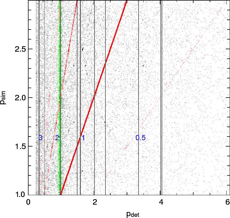
Figure 20: Density plot of simulated period $p_{sim}$ against detected period $p_{det}$ for Jovian planets with periods between 1-3 days after application of our alias removal. Marked in red are the lines for correct period identification and corresponding aliases (blue number) or half, double and triple the simulated period. Further marked in green is a period area with a high amount of false detection contaminations, removed period regions (see Tab. 3) are marked as horizontal grey lines.

Marked in the same Fig. is a region around 1 day that shows an increased number of detections but is outside of our clipping limits, marked in green. While we remove the large peak around 1.00 days, shown in Fig. 18, we cannot completely remove the area between about 0.9 to 1.1 days since that would result in too many actual transits being clipped out.
With a sample of more than 4 million light curves overall and more than 60000 M dwarfs, it is necessary to eliminate a large amount of light curves before visual inspection. Many surveys use a S/N criterion for preselection, however, this can be improved upon.
We take a set of simulated light curves, correct periods already selected, and set up the unmodified set of light curves as the training sample. Before starting the simulation, we remove our planetary candidates from the list of simulation targets. We take the reasonable assumption that even if there is a remaining undiscovered planetary signal in the sample, the effect will be negligible since the set consists of more than 60000 light curves.
We optimize the selection criteria that we then use on the real data. Using the same approach as Zendejas Dominguez et al. (2013), we set up a grid of over 100000 possible combinations of parameters, including S/N, transit depth, transit v shape and transit duration. We settle on the criteria that are shown in table 4 in Sect. 5. Besides S/N, criteria for the number of points in the transit, to rule out random noise detections, and criteria for transit duration and depth, to filter out obvious eclipsing binaries, have shown to be very effective in reducing the number of false detections.
As a last step we account for the visual selection bias. A signal that has been detected with the correct period and passed all of the selection criteria could still be disregarded in our visual inspection in case of only a partially visible transit. We implement a visual bias filter that eliminates folded transit light curves that show gaps during the eclipse, something which would lead us to dismiss the candidate in the real sample. In order to optimize this algorithm, we preselect an arbitrary set of 200 planet-injected light curves with periods of 1-10 days. We mark those that we would accept and those we would rule out and then recreate those results with our automatic filter. This visual bias filter removes about 8% of the remaining light curves.
We optimize this process for a number of 60 remaining light curves per field while recovering as many simulated objects as possible. The results are shown in table 4. This number is the best compromise, based on our simulations. Decreasing it will impact our detection efficiency while increasing it will not give us additional detections.

5 SURVEY STATUS

The complete data reduction for Pan-Planets has been finished and all light curves have been created as described in detail in Sect. 2.2. We use our trapezoidal box fitting algorithm to identify the best planet candidates in our data. As described in the previous Sect., we use the simulated data for optimizing the selection criteria in order to retain about 60 light curves per field for visual inspection. The impact of each criterion for the M dwarf sample is listed in table 4.

Criterion	Remaining	Removed	Change
Input	65258	-	-
Alias clipping	57054	8204	-12.6%
S/N $\geq$ 12	5490	51564	-90.4%
Transit points $\geq$ 15	5072	418	-7.61%
Transit duration $\leq$ 0.1	599	4473	-88.2%
Transit depth $\leq$ 0.15	553	46	-7.76%
Transit v shape $\leq$ 0.7	535	18	-3.10%
Secondary S/N $\leq$ 10	419	116	-21.8%

Table 4: List of selection criteria and their impact on the M dwarf light curve signal detection. S/N and transit duration served as criteria with the highest impact, the former for eliminating false detections from random noise patterns, the latter for separation from binaries.

Examples for several categories of interest are listed below in Sect. 5.2. Overall, we have 8 candidates around M stars, mostly hot Jupiters, 10 additional candidates around hotter stellar types, more than 300 M dwarf binary systems and 11 white dwarf variable systems.

5.1 Follow-up

We are in the process of following up our candidates through a variety of observatories. Since this process is ongoing, we show only an exemplary candidate per category in the next Sect. For low-resolution follow-up, we obtained spectroscopic data from the Hobby Eberly Telescope 9.2m Low Resolution Spectrograph (HET LRS) (Ramsey et al., 1998; Hill et al., 1998), Calar Alto 2.2m CAFOS (Patat & Taubenberger, 2011) and McDonald 2.1m ES2 spectrograph (Ries & Riddle, 2014). The data are being processed and a sample spectrum has been shown in Sect. 3.6. We use the low-resolution spectra to characterize the host stars and compare the results to the SED fitting predictions. Further, we use the data to rule out binary stars, which possess a radial velocity amplitude that is measurable even in low resolution spectra.
All planet candidates are being observed during their predicted transit phase with the new 2m Fraunhofer Telescope Wendelstein (Hopp et al., 2014) in order to improve the period accuracy, using the wide field imager (Kosyra et al., 2014). The high-precision photometric data also allows us to improve the fitting of the transit shape, further ruling out false detections from red noise residuals and eclipsing binaries. Our predicted transit times have excellent accuracy with a deviation of less than 15 minutes over the course of three years without additional observations. As the next stage, we will record the transits again but in a wide range of photometric bands, allowing us to gain further insight into the physical parameters of this system.
The final step will be high-precision radial velocity measurements to eliminate all possibilities of false-positive detections, i.e. background eclipsing binary blends or brown dwarfs, and determine the mass of the planets. We are in the process of preparing those observations for the most promising candidates.

5.2 Candidates

After the identification of the planet candidates with the trapezoidal box fitting, we perform a more comprehensive fit. We determine limb darkening parameters (Claret & Bloemen, 2011) from SED fitting and subsequently fit planetary/stellar radius, period, t0 and inclination with a Monte-Carlo approach, further taking additional observations from Wendelstein 2m (Hopp et al., 2014) into account. We display an exemplary candidate for each of the four primary categories of interest: hot Jupiters around M dwarfs, hot Jupiters around main-sequence stars, M-dwarf binary systems and other variable systems of interest.
Candidate 4.03-05317, shown in Fig. 21, is one of the prime planet candidates for follow-up analysis. The host star seems to be a M0 dwarf with an effective temperature of about 3950 K and a radius of about 0.55 $R_{\odot}$, which is in good agreement with the best fit for the transit shape. With radius estimates between 0.96 and 1.17 R_J and an extremely short period of 0.416 d, it is quite uncommon and has a closer orbit than all known hot Jupiters.

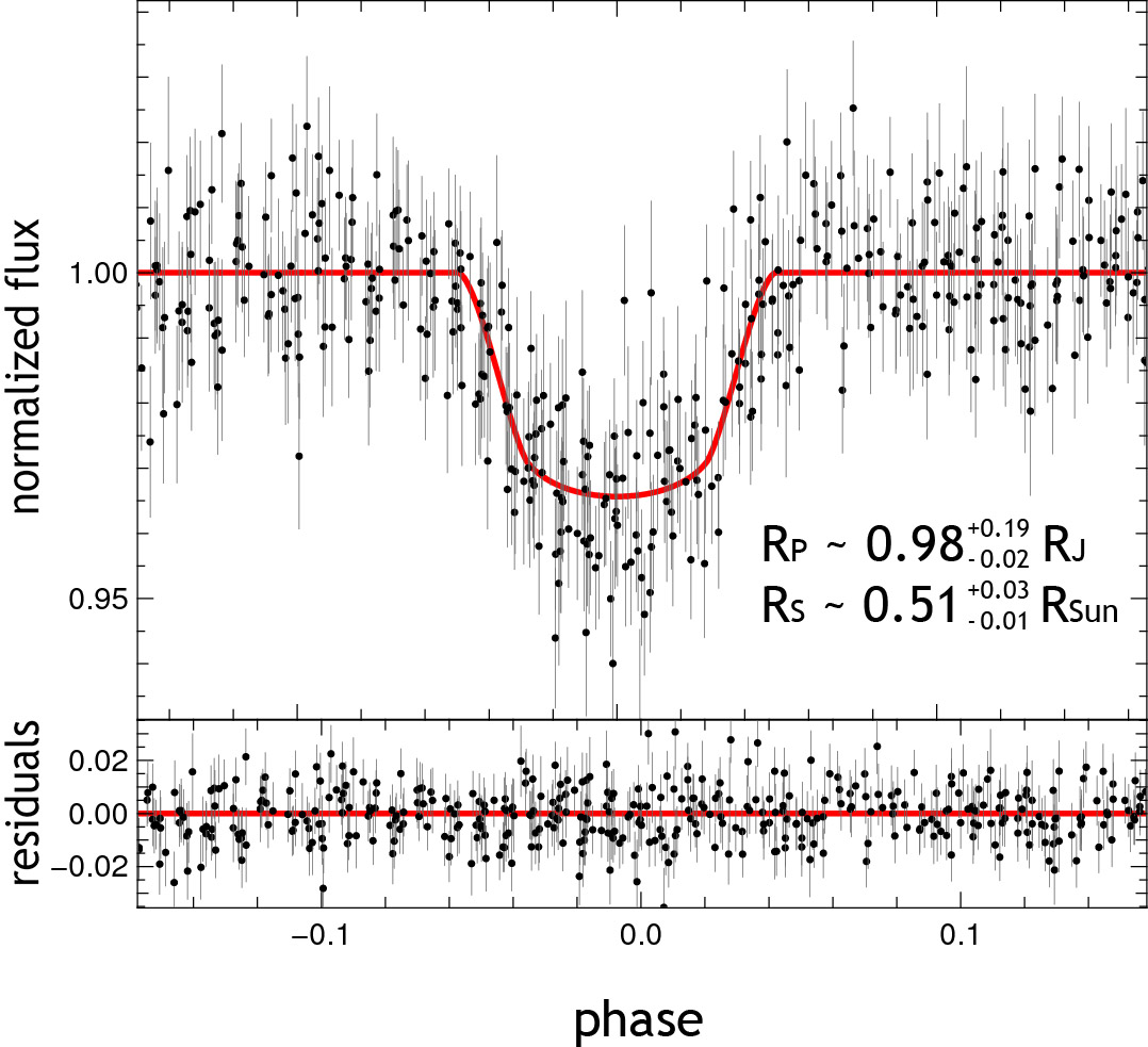
Figure 21: Folded light curve (p=0.416 d) of planetary candidate 403-05317. The red line shows the best fit for parameters inclination, period, t0, planetary and stellar radii. The lower panel shows the residuals from the fit.

Candidate 1.40-14711, shown in Fig. 23 and 22, exhibits a clean transit signal with the most likely scenario being a hot Jupiter that is transiting in front of a late K type star with an effective temperature of about 4200 K. We followed up this candidate with the 2m Fraunhofer Telescope Wendelstein (Hopp et al., 2014), using the wide field imager (Kosyra et al., 2014). One of the resulting light curves is shown in Fig. 22.

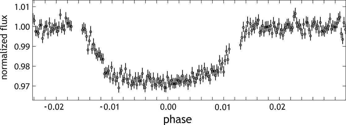
Figure 22: Transit of planetary candidate 1.40-14711, recorded with the wide field imager on the Wendelstein Fraunhofer 2m telescope in the i-band. Exposure times were 30 seconds.

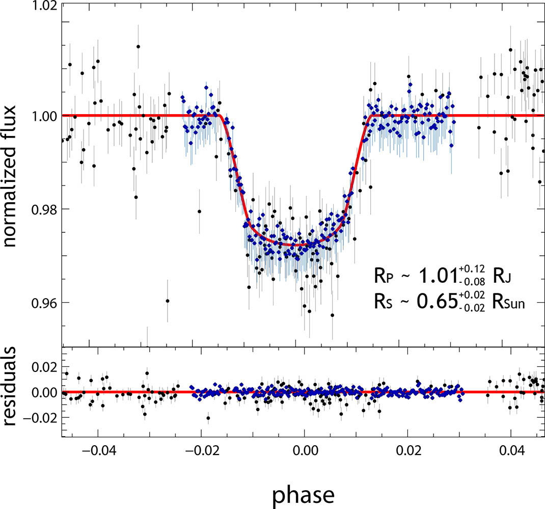
Figure 23: Folded light curve (p=2.663 d) of planetary candidate 1.40-14711. The red line shows the best fit for parameters inclination, period, t0, planetary and stellar radii. The lower panel shows the residuals from the fit. The fit includes the additional data that were taken with the 2m Fraunhofer Telescope Wendelstein (blue diamonds) besides the original Pan-Planets data (black circles).

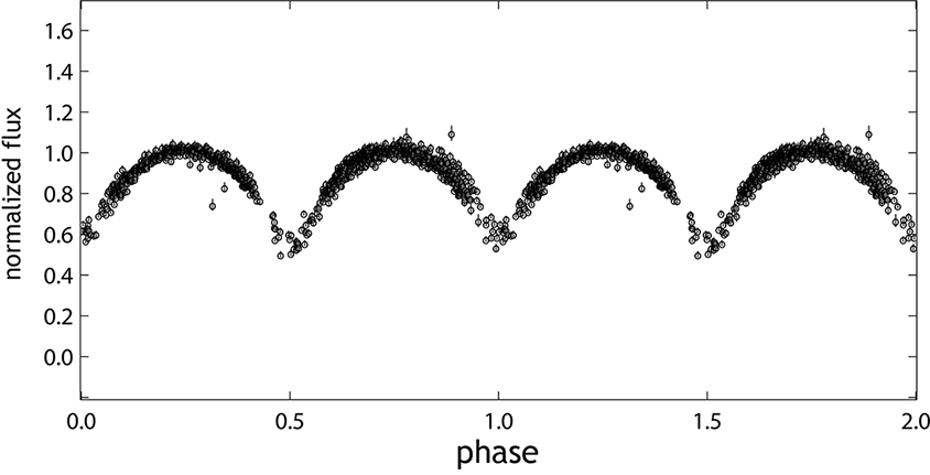
Figure 24: Folded light curve (p=0.23 d) of eclipsing binary 134-18802. The period of this binary system is extremely short (compare Norton et al. (2011)). The system likely consists of two similar-sized M dwarfs that are semi-detached. Note that the light curve is displayed over two phases for better visibility of the features.

Candidate 1.34-18802, shown in Fig. 24, is one of many short-period (p=0.23 d) eclipsing M dwarf binary systems that we found. With light drops of 43% and 41% for the primary and secondary eclipse, respectively, the two members of this system seem to be of similar size and about M1 spectral type.

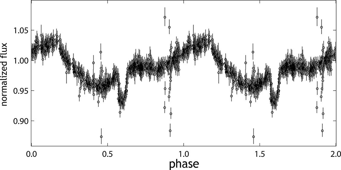
Figure 25: Folded light curve (p=2.633 d) of the unusual variable system 0.50-06948. The eclipse does not occur at phase 0.5 of the somewhat sinusoidal variation. Note that the light curve is displayed over two phases for better visibility of the features.

Candidate 0.50-06948, shown in Fig. 25, is a remarkable variable system that was found in the Pan-Planets data. There are strong periodic variations, coherent over the course of four years, with an eclipse event located offset from the minimum of the variation. SED fitting predicts an high effective temperature of about 10000 K. We recorded a spectrum with ES2 spectrograph at the McDonald observatory, confirming that the system exhibits broad Balmer-lines with an otherwise continuous spectrum. As of now the exact nature of this system is unclear.

6 Discussion

6.1 Detection Efficiency

For each planet population, we repeat 100 simulation runs per M dwarf and 40 runs per FGK star. This adds up to 50 million individual runs per planet population for M dwarfs and 245 million runs for the K, G and F star population. We end up with a recovery ratio for the individual planetary populations shown in table 5. One can see that the detection efficiency is increasing strongly for lower periods and larger radii. A histogram of the detection efficiency against the period for M dwarfs can be seen in Fig. 26 on the top panel.

M dwarf	Simulated	Recovered	Efficiency
VHJ	772870	45.6%	40.6%
HJ	471484	17.5%	14.5%
WJ	198983	7.3%	5.45%
VHS	772044	19.8%	18.5%
VHN	767916	10.3%	9.68%
K, G, F dwarf
VHJ	2476929	9.32%	8.72%

Table 5: Detection efficiencies for different planet populations. For M dwarfs, we use all 65258 targets minus the 8 planet candidates, for KGF dwarfs we use 460910 targets, excluding the planet candidates. The percentage of recovered planets is calculated by normalizing the number of correct detections by the number of possible detections (see Eq. 4). The efficiency is determined after selection criteria, alias clipping and visual bias filter have been applied to the results from the BLS analysis. For smaller stellar radii, larger planetary radii and shorter periods, the efficiency is higher.

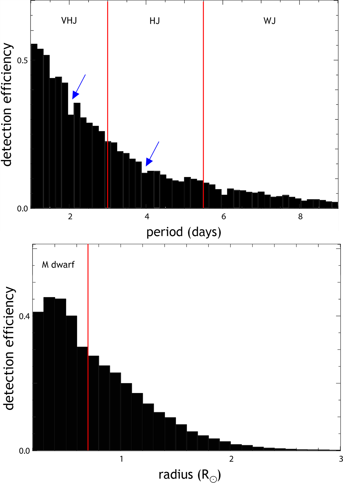
Figure 26: Top: Detected period against detection efficiency for all hot Jupiter populations around M dwarfs (divided by red lines). One can see two gaps at 1.6 and 4.0 days, resulting from our alias detection removal (blue arrows). Bottom: Histogram of stellar radius against detection efficiency. We combined the results from the M dwarf VHJ simulation and the VHJ simulations for hotter dwarf stars (divided by red line).

One has to keep in mind that the recovery efficiencies shown in table 5 include possible cases of barely observable transits - even the slightest overlaps between planet and star are being simulated where the transit would take place within only a few seconds as an extreme example. There further are simulated light curves that are not observable due to data gaps or badly timed transits that constantly fall outside of our observing windows. Even with perfect data, it would therefore be hard to reach 100% detection efficiency. The detection efficiency in relation to the stellar radius is shown in the bottom panel of Fig. 26. It is clear that the stellar radius has a significant impact on the detection rate. The efficiency strongly decreases after 0.5 R_⊙. Since the efficiency reaches a plateau before that, we assume that this is the maximum achievable detection efficiency with Pan-Planets. The other transit signals may be lost in observation gaps or in strong stellar variability that masks the signal and cannot be properly distinguished due to an insufficient number of data points. For K, F and G dwarfs combined, we expect to detect $3.0^{+3.3}_{-1.6}$ transiting VHJs, assuming an occurrence rate of $0.1408\cdot(1^{+1.1}_{-0.54})\%$ based on the OGLE-III transit search (Gould et al., 2006).
Our large sample means that, assuming a null result in which none of the M dwarf candidates turn out to be actual planets, we can set new upper limits for the planetary occurrence rates of hot Jupiters around those stars. The number of detections is characterized with a Poisson distribution. Therefore, assuming a number of k planets in our sample, the probability of having N_det planets is

$$P_{k}=\frac{{N_{det}^{k}}}{k!}e^{-N_{det}}.$$ (8)

The geometric probability for a visible transit is empirically being accounted for in our simulations. For hot Jupiters, between 9.8% ($\mathrm{1\,d\leq p\leq 3\,d}$) to 2.5% ($\mathrm{5\,d\leq p\leq 10\,d}$) of the simulated transits pass our visibility criterion (Eq. 4). The detection efficiency is therefore a combination of the geometric probability $P_{transit}$ and the detector efficiency $P_{det}$. We now assume the null result, e.g. $k=0$. In order to compare our results to Kovács et al. (2013) and Zendejas Dominguez et al. (2013), we also use a confidence interval of 95%. Solving

$$P(N_{det}<N_{max})=\int\limits_{0}^{N_{max}}e^{-N}dN=0.95,$$ (9)

we get N_max=3. We can calculate the upper limit by replacing the number of observed planets N_det with the product of the number of stars with the detection efficiency and fraction $f$ so that $N_{det}=N_{stars}\cdot P_{det}\cdot P_{transit}\cdot f$:

$$f_{95\%}\leq\frac{3}{N_{stars}\cdot P_{det}\cdot P_{transit}}.$$ (10)

Taking the individual detection efficiencies in every field, the geometric probability for each period bin and assuming that the distribution of planetary radii is even into account, we end up with an upper limit of 0.34%. This is a significantly lower result than found in previous surveys where small sample sizes counteracted higher detection efficiencies. Splitting up the results for M0-M2 and M2-M4 sub groups as done in Kovács et al. (2013) and Zendejas Dominguez et al. (2013), we derive upper limits of 0.49% and 1.1%, respectively. However, we possess several plausible M dwarf hot Jupiter candidates. Assuming one correctly identified hot Jupiter, we calculate the occurrence rate to be 0.11${}^{+0.37}_{-0.02}$% with a 95% confidence limit. For the upper uncertainty, we integrate equation 9 in the range of 1 to $N_{max}$ and determine the fraction limit. For the lower uncertainty, we consider the scatter of our simulations and calculate the difference between the average and minimum detected planets per simulation run. It may look counter-intuitive that a successful detection lowers the supposed fraction. One has to keep in mind that the null result describes the upper limit while a successful detection allows for an estimate of the fraction. Additionally, the uncertainties of the fraction estimate are higher than the null result’s limit. As another comparison, we determine the best-case results from the Kepler survey. We assume a number of 3897 stars in the temperature range between 3000 K and 4000 K in the distribution of Dressing & Charbonneau (2013) and simulate a system with the same hot Jupiter population as ours for the given stellar radius. If the criterion

$$sin(i)<\frac{R_{star}-R_{planet}}{a},$$ (11)

e.g. a full transit of the planet, is met, we assume a successful detection due to the photometric accuracy and the long baseline of Kepler. Note that this criterion is different to eq. 4: here we assume a full eclipse of the planet. The resulting fraction with one confirmed planet (Johnson et al., 2012) is $0.17(^{+0.67}_{-0.04})$%, an occurrence rate that is on par with our own results although 50% higher and with a larger error due to the small sample of cool Kepler stars. Further, the inclusion of stars up to 4000 K means that this fraction cannot be compared directly. Furthermore, there are three additional hot Jupiter candidates in the Kepler database, KOIs 3749.01, 1654.01 and 1176.01. All of their radii are very close to that of Jupiter and show no signs of inflation, e.g. radii much larger than 1 $\mathrm{R_{J}}$ that is frequent for hot Jupiters. It is possible that they are in fact Brown Dwarfs, so further follow-up will be necessary to determine their true nature. This means that Kepler’s occurrence rate limits might end up being higher than assumed here, depending on whether or not all of the remaining Kepler candidates are planets.
We illustrate the impact of this new occurrence limit in Fig. 27. Our result pushes the upper limit down to the level of other main-sequence stars. However, theoretical models (Ida & Lin, 2005; Johnson et al., 2010; Mordasini et al., 2012) point to an even lower fraction.

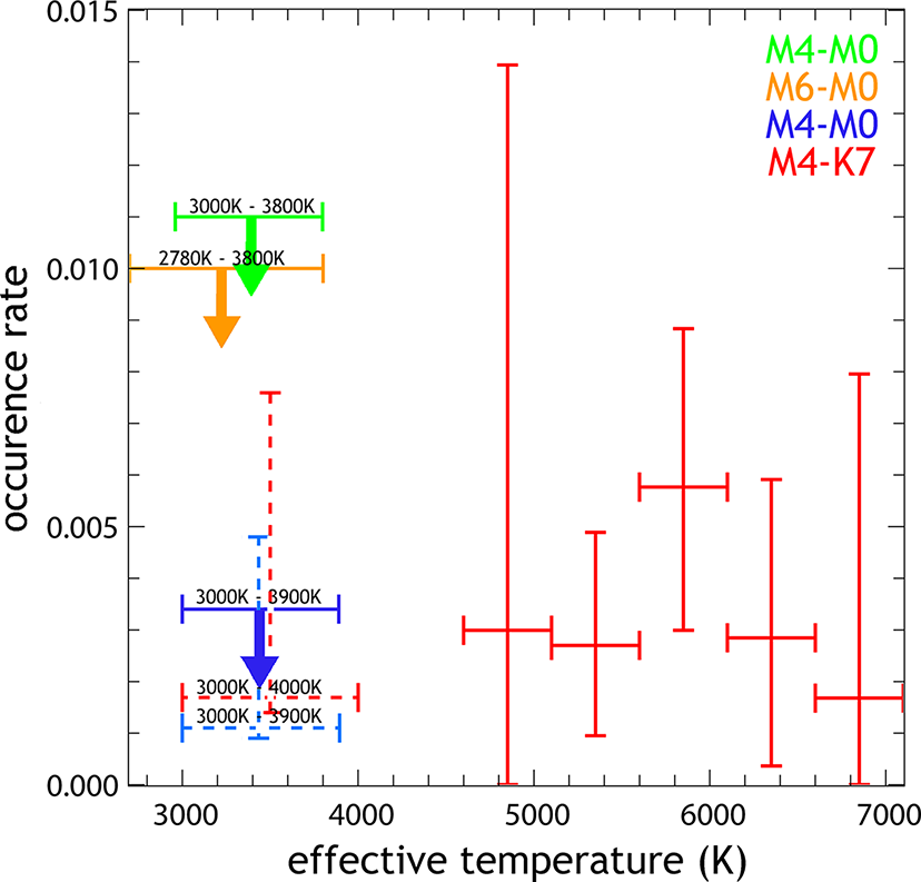
Figure 27: Adaptation of Fig. 13 in Kovács et al. (2013), showing the hot Jupiter fractions determined by different surveys. We added our new results, marked in dark blue (upper limit) and light blue dotted line (fraction in case of a successful detection). Orange shows the limits derived from radial velocity surveys (Bonfils et al., 2013), red from the Kepler survey (extracted by Kovács et al. (2013)), red in dotted lines from our own simulations for Kepler and green from the WFCAM transit survey (Zendejas Dominguez et al., 2013).

6.2 Comparison to the expected number of detections

When comparing our measured detection efficiency to the predictions of Koppenhoefer et al. (2009), one has first to consider the difference in the number of data points per star. Pan-Planets was scheduled for 4% of the total observing time, which we actually received. However, Koppenhoefer et al. (2009) assumed that this would add up to 280 h, while in the end we received 165 h because of different reasons (delayed fully operational readiness, weather, maintenance). This significantly decreased the detection efficiency. The change in observing time was shown to have a non-linear impact, e.g. doubling the amount of observing time increased the number of detected planets by a factor of three (see tables 8 and 9 in Koppenhoefer et al. (2009)) for periods longer than 3 days. Furthermore, while we assumed a precision up to 4 mmag red noise residual, the majority of light curves now has a precision between 5-10 mmag. There is no directly comparable simulation, so we would have to adjust the previous red noise models. The unforeseen issues for bright stars in 2010 could also not have been taken into account, meaning that there are less than 1500 data points for any bright source (i’ $\leq$ 15.5 mag).
We scale down table 8 in Koppenhoefer et al. (2009), which assumes 120 hours of data taken in one year, for the aforementioned effects - a red noise residual level of 5 mmag and fewer data points than previously assumed. We find our expected number of $3.0^{+3.3}_{-1.6}$ detected hot Jupiters to be consistent with the scaled estimate of 7.4$\pm$2.9 detections.

7 CONCLUSION

In the years 2010-2012, the Pan-Planets survey observed seven overlapping fields in the Galactic disk for about 165 hours. The main scientific goal of the project is to find transiting planets around M dwarfs, however, with more than 4 million sources brighter than i’=18 in the 42 sq. deg. survey area the data are a valuable source for a diversity of scientific research.
We established an efficient procedure to determine the stellar parameters $\mathrm{T_{eff}}$ and log $g$ of all sources using a method based on SED fitting, utilizing a three-dimensional dust map and proper motion information. In this way we were able to identify more than 65 000 M dwarfs which is by far the biggest sample of low-mass stars observed in a transit survey up to now.
Using a optimized difference imaging data processing pipeline we reached a photometric precision of 5 mmag at the bright end at around $i_{P1}$ = 15 mag. This makes Pan-Planets sensitive to short period hot Jupiters and hot Neptunes around M dwarfs and short period hot Jupiters around hotter stellar types.
To search for planetary transits we used a modified BLS algorithm. We applied several selection criteria which have been optimized using Monte-Carlo simulations in order to reduce the number of visually inspected light curve from several million down to a about 60 per field. We detected several planet candidates around M dwarfs and hotter stars which are currently being followed up. In addition, we found many interesting low-mass eclipsing binaries and eclipsing white dwarf systems which we will study in detail in the current observing season.
Using Monte-Carlo simulations we determined the detection efficiency of the Pan-Planets survey for several stellar and planetary populations. We expect to find $3.0^{+3.3}_{-1.6}$ hot Jupiters around F, G and K dwarfs with periods lower than 10 days based on the planet occurrence rates derived in previous surveys. For M dwarfs, the fraction of stars with a hot Jupiter is under debate. With the large sample size of Pan-Planets, we were able to determine a planet fraction of $0.11(^{+0.37}_{-0.02})$% in case one of our candidates turns out to be a real detection. For this result, we considered the average detection rate of the simulations and compared the scatter at a 95% confidence.
If however none of our candidates is real, we were able to put a 95% confidence upper limit of 0.34% on the hot Jupiter occurrence rate of M dwarfs. This limit is higher than the calculated fraction in case of a successful detection, however, the uncertainties of the fraction are in turn higher than this upper limit. This result is a significant improvement over previous estimates where the lowest limit published so far is 1.1%, found in the WTS survey (Zendejas Dominguez et al., 2013), or, using our approach to estimate the generous best case for Kepler, $0.17(^{+0.67}_{-0.04})$%. Despite the significant improvement, our upper limit is still comparable to the occurrence rate of hot Jupiters around F, G and K dwarfs, even more so in case of a successful detection. The estimates from Gould et al. (2006) based on the OGLE-III transit search seem to be in good agreement with our new limits. Therefore we could not yet confirm the theoretical prediction of a lower rate for cool stars. Other surveys with even larger M dwarf samples and/or better detection efficiency will be needed to answer this question.

References

- Alard & Lupton (1998) Alard, C. & Lupton, R. H. 1998, ApJ, 503, 325
- Allard et al. (2012) Allard, F., Homeier, D., & Freytag, B. 2012, Royal Society of London Philosophical Transactions Series A, 370, 2765
- Baraffe et al. (2015) Baraffe, I., Homeier, D., Allard, F., & Chabrier, G. 2015, A&A, 577, A42
- Begeman et al. (2013) Begeman, K., Belikov, A. N., Boxhoorn, D. R., & Valentijn, E. A. 2013, Experimental Astronomy, 35, 1
- Bonfils et al. (2013) Bonfils, X., Delfosse, X., Udry, S., et al. 2013, A&A, 549, A109
- Bressan et al. (2012) Bressan, A., Marigo, P., Girardi, L., et al. 2012, MNRAS, 427, 127
- Chen et al. (2014) Chen, Y., Girardi, L., Bressan, A., et al. 2014, MNRAS, 444, 2525
- Christiansen et al. (2015) Christiansen, J. L., Clarke, B. D., Burke, C. J., et al. 2015, ApJ, 810, 95
- Claret & Bloemen (2011) Claret, A. & Bloemen, S. 2011, A&A, 529, A75
- Dawson & Murray-Clay (2013) Dawson, R. I. & Murray-Clay, R. A. 2013, ApJ, 767, L24
- Deacon et al. (2015) Deacon, N. R., Kraus, A. L., Mann, A. W., et al. 2015, ArXiv e-prints
- Dotter et al. (2008) Dotter, A., Chaboyer, B., Jevremović, D., et al. 2008, ApJS, 178, 89
- Dressing & Charbonneau (2013) Dressing, C. D. & Charbonneau, D. 2013, ApJ, 767, 95
- Dressing & Charbonneau (2015) Dressing, C. D. & Charbonneau, D. 2015, ApJ, 807, 45
- Duda & Hart (1972) Duda, R. O. & Hart, P. E. 1972, Commun. ACM, 15, 11
- Fischer & Valenti (2005) Fischer, D. A. & Valenti, J. 2005, ApJ, 622, 1102
- Gaidos & Mann (2014) Gaidos, E. & Mann, A. W. 2014, ApJ, 791, 54
- Gonzalez (1997) Gonzalez, G. 1997, MNRAS, 285, 403
- Gössl & Riffeser (2002) Gössl, C. A. & Riffeser, A. 2002, A&A, 381, 1095
- Gould et al. (2006) Gould, A., Dorsher, S., Gaudi, B. S., & Udalski, A. 2006, Acta Astron., 56, 1
- Green et al. (2015) Green, G. M., Schlafly, E. F., Finkbeiner, D. P., et al. 2015, ApJ, 810, 25
- Hartman et al. (2014) Hartman, J. D., Bayliss, D., Brahm, R., et al. 2014, ArXiv e-prints
- Hartman et al. (2009) Hartman, J. D., Gaudi, B. S., Holman, M. J., et al. 2009, ApJ, 695, 336
- Henry et al. (2006) Henry, T. J., Jao, W.-C., Subasavage, J. P., et al. 2006, AJ, 132, 2360
- Hill et al. (1998) Hill, G. J., MacQueen, P. J., Nicklas, H., et al. 1998, in Bulletin of the American Astronomical Society, Vol. 30, American Astronomical Society Meeting Abstracts, 1262
- Hodapp et al. (2004) Hodapp, K. W., Kaiser, N., Aussel, H., et al. 2004, Astronomische Nachrichten, 325, 636
- Hopp et al. (2014) Hopp, U., Bender, R., Grupp, F., et al. 2014, in Society of Photo-Optical Instrumentation Engineers (SPIE) Conference Series, Vol. 9145, Society of Photo-Optical Instrumentation Engineers (SPIE) Conference Series, 2
- Ida & Lin (2005) Ida, S. & Lin, D. N. C. 2005, Progress of Theoretical Physics Supplement, 158, 68
- Johnson et al. (2010) Johnson, J. A., Aller, K. M., Howard, A. W., & Crepp, J. R. 2010, PASP, 122, 905
- Johnson & Apps (2009) Johnson, J. A. & Apps, K. 2009, ApJ, 699, 933
- Johnson et al. (2007) Johnson, J. A., Butler, R. P., Marcy, G. W., et al. 2007, ApJ, 670, 833
- Johnson et al. (2012) Johnson, J. A., Gazak, J. Z., Apps, K., et al. 2012, AJ, 143, 111
- Kaiser et al. (2002) Kaiser, N., Aussel, H., Burke, B. E., et al. 2002, in Society of Photo-Optical Instrumentation Engineers (SPIE) Conference Series, Vol. 4836, Survey and Other Telescope Technologies and Discoveries, ed. J. A. Tyson & S. Wolff, 154–164
- Koppenhoefer et al. (2009) Koppenhoefer, J., Afonso, C., Saglia, R. P., & Henning, T. 2009, A&A, 494, 707
- Koppenhoefer et al. (2013) Koppenhoefer, J., Saglia, R. P., & Riffeser, A. 2013, Experimental Astronomy, 35, 329
- Kosyra et al. (2014) Kosyra, R., Gössl, C., Hopp, U., et al. 2014, Experimental Astronomy, 38, 213
- Kovács et al. (2013) Kovács, G., Hodgkin, S., Sipőcz, B., et al. 2013, MNRAS, 433, 889
- Kovács et al. (2002) Kovács, G., Zucker, S., & Mazeh, T. 2002, A&A, 391, 369
- Magnier (2006) Magnier, E. 2006, in The Advanced Maui Optical and Space Surveillance Technologies Conference, 50
- Mann et al. (2013) Mann, A. W., Gaidos, E., Kraus, A., & Hilton, E. J. 2013, ApJ, 770, 43
- Mann et al. (2012) Mann, A. W., Gaidos, E., Lépine, S., & Hilton, E. J. 2012, ApJ, 753, 90
- Monet et al. (2003) Monet, D. G., Levine, S. E., Canzian, B., et al. 2003, AJ, 125, 984
- Montet et al. (2014) Montet, B. T., Crepp, J. R., Johnson, J. A., Howard, A. W., & Marcy, G. W. 2014, ApJ, 781, 28
- Mordasini et al. (2012) Mordasini, C., Alibert, Y., Benz, W., Klahr, H., & Henning, T. 2012, A&A, 541, A97
- Morton & Swift (2014) Morton, T. D. & Swift, J. 2014, ApJ, 791, 10
- Neves et al. (2013) Neves, V., Bonfils, X., Santos, N. C., et al. 2013, A&A, 551, A36
- Norton et al. (2011) Norton, A. J., Payne, S. G., Evans, T., et al. 2011, A&A, 528, A90
- Patat & Taubenberger (2011) Patat, F. & Taubenberger, S. 2011, A&A, 529, A57
- Petigura et al. (2013a) Petigura, E. A., Howard, A. W., & Marcy, G. W. 2013a, Proceedings of the National Academy of Science, 110, 19273
- Petigura et al. (2013b) Petigura, E. A., Marcy, G. W., & Howard, A. W. 2013b, ApJ, 770, 69
- Ramsey et al. (1998) Ramsey, L. W., Adams, M. T., Barnes, T. G., et al. 1998, in Society of Photo-Optical Instrumentation Engineers (SPIE) Conference Series, Vol. 3352, Advanced Technology Optical/IR Telescopes VI, ed. L. M. Stepp, 34–42
- Ries & Riddle (2014) Ries, J. & Riddle, A. 2014, in Asteroids, Comets, Meteors 2014, ed. K. Muinonen, A. Penttilä, M. Granvik, A. Virkki, G. Fedorets, O. Wilkman, & T. Kohout, 446
- Robin et al. (2003) Robin, A. C., Reylé, C., Derrière, S., & Picaud, S. 2003, A&A, 409, 523
- Santos et al. (2001) Santos, N. C., Israelian, G., & Mayor, M. 2001, A&A, 373, 1019
- Schlafly & Finkbeiner (2011) Schlafly, E. F. & Finkbeiner, D. P. 2011, ApJ, 737, 103
- Schlegel et al. (1998) Schlegel, D. J., Finkbeiner, D. P., & Davis, M. 1998, ApJ, 500, 525
- Skrutskie et al. (2006) Skrutskie, M. F., Cutri, R. M., Stiening, R., et al. 2006, AJ, 131, 1163
- Tamuz et al. (2005) Tamuz, O., Mazeh, T., & Zucker, S. 2005, MNRAS, 356, 1466
- Tomaney & Crotts (1996) Tomaney, A. B. & Crotts, A. P. S. 1996, AJ, 112, 2872
- Tonry & Onaka (2009) Tonry, J. & Onaka, P. 2009, in Advanced Maui Optical and Space Surveillance Technologies Conference, 40
- Tonry & Pan-STARRS Team (2005) Tonry, J. & Pan-STARRS Team. 2005, in Bulletin of the American Astronomical Society, Vol. 37, American Astronomical Society Meeting Abstracts, 121.01
- Torres-Dodgen & Weaver (1993) Torres-Dodgen, A. V. & Weaver, W. B. 1993, PASP, 105, 693
- Triaud et al. (2013) Triaud, A. H. M. J., Anderson, D. R., Collier Cameron, A., et al. 2013, A&A, 551, A80
- West et al. (2011) West, A. A., Morgan, D. P., Bochanski, J. J., et al. 2011, Astronomical Journal, 141, 97
- Winters et al. (2015) Winters, J. G., Henry, T. J., Lurie, J. C., et al. 2015, AJ, 149, 5
- Wright et al. (2010) Wright, E. L., Eisenhardt, P. R. M., Mainzer, A. K., et al. 2010, AJ, 140, 1868
- Zendejas Dominguez et al. (2013) Zendejas Dominguez, J., Koppenhoefer, J., Saglia, R. P., et al. 2013, A&A, 560, A92