Multi Currency Credit Default Swaps

Abstract

Credit Default Swaps (CDS) on a reference entity may be traded in multiple currencies, in that protection upon default may be offered either in the currency where the entity resides, or in a more liquid and global foreign currency. In this situation currency fluctuations clearly introduce a source of risk on CDS spreads. For emerging markets, but in some cases even in well developed markets, the risk of dramatic Foreign Exchange (FX) rate devaluation in conjunction with default events is relevant. We address this issue by proposing and implementing a model that considers the risk of foreign currency devaluation that is synchronous with default of the reference entity. As a fundamental case we consider the sovereign CDSs on Italy, quoted both in EUR and USD.

Preliminary results indicate that perceived risks of devaluation can induce a significant basis across domestic and foreign CDS quotes. For the Republic of Italy, a USD CDS spread quote of 440 bps can translate into a EUR quote of 350 bps in the middle of the Euro–debt crisis in the first week of May 2012. More recently, from June 2013, the basis spreads between the EUR quotes and the USD quotes are in the range around 40 bps.

We explain in detail the sources for such discrepancies. Our modeling approach is based on the reduced form framework for credit risk, where the default time is modeled in a Cox process setting with explicit diffusion dynamics for default intensity/hazard rate and exponential jump to default. For the FX part, we include an explicit default–driven jump in the FX dynamics. As our results show, such a mechanism provides a further and more effective way to model credit / FX dependency than the instantaneous correlation that can be imposed among the driving Brownian motions of default intensity and FX rates, as it is not possible to explain the observed basis spreads during the Euro–debt crisis by using the latter mechanism alone.

AMS Classification Codes : 60H10, 60J60, 91B70;

JEL Classification Codes : C51, G12, G13

Keywords: Credit Default Swaps, Liquidity spread, Liquidity pricing, Intensity models, Reduced Form Models, Capital Asset Pricing Model, Credit Crisis, Liquidity Crisis, Devaluation jump, FX devaluation, Quanto Credit effects, Quanto CDS, Multi currency CDS.

1 Introduction

1.1 Overview of the Modelling Problem

The need for quanto default modeling arises naturally when pricing credit derivatives offering protection in multiple currencies.

Reasons for entering into Credit Default Swaps (CDS) in different currencies can come from financial, economic, or even legislative considerations: they range from the composition of the portfolio that has to be hedged to the accounting rules in force in the country where the investor is based. In case the reference entity is sovereign, economic reasons play a major role since for an investor it might be more appealing to buy protection on, for example, Republic of Italy’s default in USD rather than in EUR. Indeed, in the latter case the currency value itself is strongly related with the reference entity’s default.

Figure 1 shows the time series of par–spreads for USD–denominated and EUR–denominated CDSs on Republic of Italy from the beginning of 2011 until the end of 2013. The time range has been chosen so to include the 2011 Euro–debt crisis.

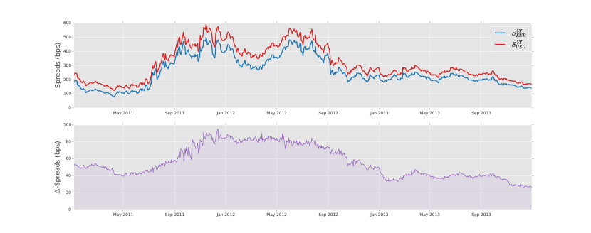
Figure 1: In the top chart, 5Y par spread time series for USD–denominated CDSs, $S_{\textrm{USD}}^{5Y}$, and EUR–denominated CDSs, $S_{\textrm{EUR}}^{5Y}$, on Italy. The difference between the two par–spreads is showed in the bottom chart.

The difference between the par–spreads for USD–denominated and EUR–denominated CDSs is shown in the bottom chart. In order to build a model which accounts for the default information and generate the spreads in the two currencies, the joint evolution of the obligors hazard rate and of the FX rate between the two currencies must be modelled.

In the present paper we show two ways to model the joint dynamics of credit and FX rates. In the first approach the interaction between the credit and the FX component is entirely explained by an instantaneous correlation between the Brownian motions driving the stochastic hazard rate and the FX rate. In a second, more sophisticated modelling approach, a further source of dependence between the two components is introduced in the form of a conditional devaluation jump of the FX rate upon default of the reference obligor.

The diffusive approach emphasizes the limitations of confining the credit/market interaction to instantaneous correlation between hazard rate and market risk factors. As shown by comparing the model–implied quanto spreads in Figure 5 with the observed quanto spreads in Figure 1, instantaneous correlation alone is not able to explain the observed quanto spread. This phenomenon is akin to the pricing of credit correlation instruments where it has been observed that instantaneous correlation between hazard rates is unable to generate the sufficient level of dependence to hit the market spreads of index tranches (see, for example, Brigo et al. (2013); Brigo and Mercurio (2006); Cherubini et al. (2004)).

Using the latter modelling approach we will show how the introduction of jump–to–default effects achieves a much stronger FX/Credit dependence than correlated Brownian motions. In particular, the addition of FX jumps allows to recover both the EUR and the USD spreads (see the results presented in Section 3.5). Furthermore, we show a powerful, yet simple, way of extracting the magnitude of currency devaluation upon default from the CDS market data (see Section 3.5.2).

In addition to multi–currency CDSs, the quanto effect in credit modelling finds a natural application in the credit valuation adjustment (CVA) space. CVA is an adjustment to the fair value of a derivative contract that accounts for the expected loss due to the counterparty’s default. We refer the interested reader to Brigo et al. (2013) for a comprehensive overview of CVA modelling and to Cherubini (2005) for specific discussions about collateral modelling. Modelling the dependence between credit and market risk factors is crucial to accurately calculate the CVA charge. One of the main challenges in calculating CVA is the lack of liquid CDS market data to calibrate model parameters. The calibration and approximation techniques showed in this paper to connect currency devaluation with multi–currency CDS par–spreads can as well be applied to CVA modelling — for example, to better reflect right–way or wrong–way risk. The resulting FX/Credit cross modelling improvement is crucial, especially in those cases where the interaction between the counterparty credit and the FX component is strong, i.e. with emerging market credits and systemically relevant counterparties.

In Section 2.5, we show how the introduction of default–driven FX jumps changes the dynamics of the stochastic hazard rate after a measure change. This happens because, from a mathematical perspective, the FX rate is a component of the Radon–Nikodym derivative that links the risk neutral probability measures associated to two different currencies. As stated by Girsanov Theorem (see , for example, Jeanblanc et al. (2009)), the dynamics of the compensated default process under different risk–neutral measures differ in their drift component. Such drift depends on the quadratic covariation between the FX rate and the default process (and it is zero when such covariation is null) and can be interpreted as the stochastic hazard rate of the reference entity.

The above result is strongly linked to another aspect of FX rate modelling, which we will refer to as FX symmetry throughout this document (see the discussion in section 2.2). Consistency between an FX rate process and its reciprocal is not guaranteed under every possible distributional assumptions made on its dynamics. For example, in case of stochastic volatility FX modelling, the reciprocal FX rate would not necessarily have the same dynamics that one would expect given that the reciprocal FX rate is also a Radon–Nikodym derivative. For geometric Brownian motions, however, this consistency is guaranteed. Due to the change in the hazard rate in the second pricing measure induced by the jump–to–default feature of the FX rate/Radon–Nikodym derivative process, we prove in section 2.5.4 that the symmetry is preserved also for our specific FX model.

1.2 Previous Literature

We refer to Bielecki et al. (2005) for an overview of the general problem of deducing a PDE to price defaultable claims and to Bielecki et al. (2008) for the specific problem of CDS hedging in a reduced–form framework.

For an introduction to the joint modelling of credit and FX in a reduced–form framework with application to Quanto–CDS pricing, we refer to Ehlers and Schönbucher (2006); EL-Mohammadi (2009). Ehlers and Schönbucher (2006) propose the idea to link FX and hazard rate by considering a jump–diffusion model for the FX–rate process where the jump happens at the default time. Differently from the present work, no explicit derivation of the PDE is presented, as the focus is on affine processes modelling.

The same idea is presented and developed in EL-Mohammadi (2009). In that work it is shown how to calculate quanto–corrected survival probabilities using a PDE–based approach. In order to do that, the author deduces a Fokker–Planck equation for the joint distribution of FX and hazard rate.

The approach we present in Section 2 below is based on the same Jump–to–Default framework as the one used in the references above. In our case, however, the calculation of the quanto–corrected survival probabilities depends on solving a Feynman–Kac equation, the solution of which is a price, while in EL-Mohammadi (2009) a probability density distribution was calculated. At implementation level, the difference between the two approaches lies in the fact that in the latter case an additional integration step would be required to calculate a price. Additionaly, the way we work out our main pricing equation makes clear what instruments and in what amounts one would need to effectively implement a delta–hedging strategy.

An algorithm using a fixed–point approach has been recently proposed to calculate CVA in Kim and Leung (2016).

The techniques showed in this paper seem particularly relevant for long–maturity trades, where the effects of idiosyncratic jump–to-default components on counterparty risk can be more pronounced and where, therefore, they can have a big impact on wrong ray risk estimation. For a relevant example of CVA calculations related to long–maturity trades, we refer to Biffis et al. (2016), where the cost of CVA and collateralization are calculated for longetivity swaps.

The use of Lévy processes with local volatility to price options on defaultable assets has been recently explored in Lorig et al. (2015), where a family of asymptotic expansions for the transition density of the underlying is derived. Differently from the approach presented in this paper, in that case a single stochastic process drives both the default intensity and the option’s underlying. On the other hand, being able to account for the implied volatility skew is feature currently missing from the framework presented in Section 2 and that will be explored in future works.

With respect to the Republic of Italy’s test case that is presented in the results’ section 3, we note that the Euro–area situation presents interesting problems that go beyond the mere credit–FX interaction which is the focus of the present work. An additional layer of complexity is provided in this case by the interconnectedness between the credit risk of the different currencies.

Empirically, Germany quanto CDS basis tends to be more pronounced than the Greece one (see Pykthtin and Sokol (2013)), reflecting higher correlation between EUR/USD and Germany hazard rate of default and higher EUR/USD devaluation upon Germany default.

1.3 Quanto CDS

Quanto CDS are designed to provide protection upon default of a certain entity in a given currency. There are cases, like for sovereign entities or for systemically important companies, when an investor might prefer to buy protection on a currency other than the one in which the assets of the reference entity are denominated. A typical reason for entering this type of trades would be to avoid the FX risk linked to the devaluation effect associated to the reference entity’s default.

Alternatively, protection might be needed in a different currency from the one in which the assets of the reference entity are denominated because it serves as a hedge on a security denominated in that specific currency.

The discounted cashflows of the premium leg, $\Pi^{\textrm{Premium}}$, are given (as seen from the protection seller’s perspective) by

$$\Pi^{\textrm{Premium}}=S^{c}\sum_{i=0}^{N}\mathbbm{1}_{\tau>T_{i}}D_{0}^{ccy}(T_{i})$$ (1)

where

• $(T_{0},\dots,T_{N})$ is the set of quarterly spaced payment times;

• $D_{t}^{ccy}(T)$ is the stochastic discount factor for currency $ccy$ at time $t$ for maturity $T$;

• $S^{c}$ is the contractual spread;

• $\tau$ is the default time of the reference entity.

The protection leg is made of a single cash flow, $\Pi^{\textrm{Protection}}$, paid upon default of the reference entity on a reference obligation:

$$\Pi^{\textrm{Protection}}=\operatorname{LGD}\mathbbm{1}_{\tau\leq T_{N}}D_{0}^{ccy}(\tau),$$ (2)

where

• $\operatorname{LGD}$ is the loss given default related to the contract.

The spread $S^{c}$ that makes the expected value of the cash–flows in Eq (1) equal to the expected value of the cash–flow in Eq (2) is referred to as par–spread and we will usually use $S$ to denote it. The existence of CDSs on the same reference entity whose premium and protection cashflows are paid in different currencies creates a basis spread between the par–spreads of these contracts. Figure 2 provides a schematic representation of two possible contracts settled in two different currencies.

Figure 2: Protection on a given reference entity can be bought by A from B in different currencies. The stream of payments in Eq (1) is indicated by the solid arrow, while the dashed arrow is used for the contingent payment in Eq (2). The $LGD$ payment, albeit settled in different currencies, is the same percentage of the notional in the two contracts.

We refer to Elizalde et al. (2010) and references therein for an overview on quanto CDS markets and for a thorough exposition of the rules governing these contracts. We note here that

• the standard contracts for sovereign CDS are denominated in USD. This means in particular that for countries of the EUR zone, like Italy, Greece or Germany, the modeling set up to use when including a devaluation approach is the one detailed in Section 2.5.5;

• upon default of the reference entity, a common auction sets the loss given default (LGD). The LGD so defined is valid for all the CDSs, irrespectively of the currency they are denominated in.

1.4 Main Contribution

In this paper, we derive the pricing equations for quanto CDS in different models within the reduced–form framework. In doing so, we show two of the main mechanisms to model dependence between the credit and the FX rate component. We will refer to the currency in which the CDSs written on the reference entity are more liquid as to the “liquid currency”, that will also define the risk neutral measure used for pricing. We will assume that CDSs in a different currency from the liquid one exist and we will refer to this second currency as the “contractual currency”. In particular, we discuss the mathematical implications of the introduction of a devaluation jump on the spot FX rate between the contractual currency and the liquid corrency, both on the pricing equations and on the main risk factors. More in detail:

1. in Proposition 1 we show that, if we assume for the FX rate defining the value of one unit of contractual currency in the liquid currency a dynamics

   $$\operatorname{d\!}Z_{t}=\mu^{Z}Z_{t}\operatorname{d\!}t+\sigma Z_{t}\operatorname{d\!}W_{t}+\gamma^{Z}Z_{t-}\operatorname{d\!}D_{t},\quad Z_{0}=z,$$ (3)

   where $D_{t}=\mathbbm{1}_{\tau<t}$ is the default process, then the hazard rates in the two currencies are linked by

   $$\hat{\lambda}_{t}=(1+\gamma^{Z})\lambda_{t};$$ (4)

   where $\hat{\lambda}$ is the hazard rate in the measure linked to the contractual currency and $\lambda$ is the hazard rate in the currency linked to the liquid currency.

   An important corollary of this result is that, in cases where CDS par–spreads can be approximated through the relation $S=(1-R)\lambda$, a similar result holds for par–spreads, too:

   $$\hat{S}=(1+\gamma^{Z})S.$$ (5)

   We show in Section 3 how such an approximation is applicable to Republic of Italy’s par–spreads in the time period ranging from 2011 to 2013;

2. in Section 2.5.4 we show that if we assume for the FX rate the dynamics given in Eq (3), then

   1. by no–arbitrage considerations, the drift of $(Z_{t},t\geq 0)$ is given by

      $$\mu^{Z}=r-\hat{r}-\gamma^{Z}\lambda_{t}(1-D_{t});$$

      where $r$ is the risk–free rate in the pricing measure linked to the liquid currency and $\hat{r}$ is the risk–free rate in the contractual measure. Alternatively, by symmetry considerations, we could model the reciprocal FX rate $X=\nicefrac{{1}}{{Z}}$ using the same type of jump–diffusion process

      $$\operatorname{d\!}X_{t}=\mu^{X}X_{t}\operatorname{d\!}t-\sigma X_{t}\operatorname{d\!}W_{t}+\gamma^{X}X_{t-}\operatorname{d\!}D_{t},\quad X_{0}=\frac{1}{z},$$

      and in this second case we would obtain a drift given by

      $$\mu^{X}=\hat{r}-r-\gamma^{X}\hat{\lambda}_{t}(1-D_{t}),$$

      where

      $$\gamma^{X}=-\frac{\gamma^{Z}}{1+\gamma^{Z}};$$

   2. in Proposition 2 we show that the no–arbitrage dynamics implied for $(X_{t},t\geq 0)$ is of the same type as the no–arbitrage dynamics of $(Z_{t},t\geq 0)$. This is a result that might not hold in general, for example when stochastic volatility is also included, or with a price–inhomogeneous local volatility model like CEV;

3. in Proposition 3 we show an approximated formula, valid for short maturity CDSs, to estimate the devaluation rate paramenter $\gamma$ and we present numerical results corroborating it in Section 3.

We study in detail the case of the currency basis spread for CDSs written on Italy in the period 2011–2013 providing, for each day in that time range, the results of the calibration of a model that includes a jump–to–default effect on the FX rate. We show the calibrated parameters and how the calibrated model parameters produce estimates which are consistent with the approximated formula in Eq (5).

2 Model Description

Our modelling framework for credit risk falls into the reduced–form approach and, as such, describes not only the evolution of survival probabilities, but also the default event.

In Section 2.1 we introduce some definitions concerning the role of different currencies involved in pricing a quanto CDS.

In Section 2.2 we introduce the general framework that we will refer to to work with two financial markets. In Section 2.3 we introduce some useful formulae and definitions to price multi currency credit default swaps.

In Section 2.4 we will model a stochastic hazard rate as a exponential Ornstein–Uhlenbeck process and the FX rate as a Geometric Brownian Motion (GBM) and we will consider the two driving diffusions to be correlated.

In Section 2.5 we present our proposal to embed a factor devaluation approach onto the FX rate dynamics. This provides a way to extend the model shown in Section 2.4.

We begin by considering a probability space $(\Omega,\mathcal{F},\mathbb{Q},(\mathcal{F}_{t},t\geq 0))$ satisfying the usual hypotheses. In particular $(\mathcal{F}_{t},t\geq 0)$ is a filtration under which the dynamics of the risk factors are adapted and under which the default time of the reference entity is a stopping–time. Depending on the specific examples, we will also consider spaces with a different equivalent measure, for example the risk neutral measure associated to the liquid money market or the risk neutral measure associated to the contractual currency money market.

We will be using a Cox process model for the default component and we will refer to the stochastic intensity of the default event simply as hazard rate or intensity, using the two terms interchangeably.

Unlike the usual approach followed in the so called “reduced–form” framework for credit risk modelling (see Lando (2004), Brigo and Mercurio (2006)), we do not introduce a second filtration with respect to which only the stochastic processes driving the market risk–factors are measurable.

2.1 The Roles of the Currencies

In this section we set up some definitions concerning the role of the currencies that will be used in our modelling approach.

For of any quanto CDS pricing, we will be considering the following two relevant currencies:

• contractual currency — This currency is a contract’s attribute: it is the currency in which both premium leg and protection leg payments are settled. When considering applications to quanto CDS, for a given reference entity, CDSs are available in at least two different contractual currencies;

• liquid currency — This is the contractual currency of the most liquidly traded CDS on a given entity. It is used to define a risk–neutral measure used to price and calibrate the model.

We list here two examples to illustrate the use of the contractual and liquid currencies.

1. the pricing in USD–measure of a CDS on Republic of Italy settled in EUR;

2. the pricing in USD–measure of a CDS on Republic of Italy settled in USD.

	Test case 1	Test case 2
Contractual currency	EUR	USD
Liquid currency	USD	USD

Table 1: Currencies involved in the priicing of the test cases detailed in Section 2.1.

We specified the values of the two currencies for each of these test cases in Table 1. We chose the test cases so that for all of them USD is the the liquid currency, but this is not necessarily true for all CDS available in multiple currencies. It is worth noting that the test case 2 can be priced using a usual single currency approach. Test cases 1 and 2 will be used in Section 3.5 to illustrate the capability of the model specified in Section 2.5.5 to explain the currency basis observed in the market.

2.2 Two Markets Measures

In this section we summarize known results about change of measure in presence of FX effects. This is mostly done to establish notation and set the scene for the following original developments.

Let us consider the two economies linked to the liquid currency and to the contractual currency, respecively. Let us also consider the corresponding money market accounts as the numeraires for both the economies. We will use a hat $\hat{\ }$, to denote variables in the contractual–currency economy, so that, for example, the two numeraires are $(B_{t},t\geq 0)$ for the liquid–currency economy and $(\hat{B}_{t},t\geq 0)$ for the contractual–currency economy. The money market accounts’ dynamics are given by

$$\operatorname{d\!}B_{t} =r_{t}B_{t}\operatorname{d\!}t,\quad B_{0}=1,$$ (6)

$$\operatorname{d\!}\hat{B}_{t} =\hat{r}_{t}\hat{B}_{t}\operatorname{d\!}t,\quad\hat{B}_{0}=1,$$ (7)

where $(r_{t},t\geq 0)$ and $(\hat{r}_{t},t\geq 0)$ are the stochastic processes describing the short rates in the two economies.

Let us also consider an exchange rate $(X_{t},t\geq 0)$ between the currencies of the two economies. $X_{t}$ is defined as the price of one unit of the liquid currency expressed as units of the foreign currency in a spot exchange at time $t$.

We are interested in finding an expression for the Radon–Nikodym derivative that changes the probability measure from $\hat{\mathbb{Q}}$ to $\mathbb{Q}$. This can be worked out by using the Change of Numeraire technique and a generic payoff denominated in the contractual currency, represented by the function $\hat{\phi}_{T}$. To do so, we consider, as said above, the contractual–currency money market account, $(\hat{B}_{t},t\geq 0)$, as a numeraire for the measure $\hat{\mathbb{Q}}$, while for the measure ${\mathbb{Q}}$ we still use the liquid–currency money market account, but with value denominated in the contractual currency, $((XB)_{t},t\geq 0)$. The price of the contractual currency payoff $\hat{\phi}$ can be expressed in the two measures as:

$$\hat{\mathbb{E}}_{t}\left[\frac{\hat{B}_{t}}{\hat{B}_{T}}\hat{\phi}_{T}\right]=\mathbb{E}_{t}\left[\frac{B_{t}X_{t}}{B_{T}X_{T}}\hat{\phi}_{T}\right].$$ (8)

The $\hat{\mathbb{E}}_{t}\left[\cdot\right]$ expectation on the left–hand side, on the other hand, can be written as

$$\hat{\mathbb{E}}_{t}\left[\frac{\hat{B}_{t}}{\hat{B}_{T}}\hat{\phi}_{T}\right]=\hat{\mathbb{E}}_{t}\left[\frac{\hat{B}_{t}B_{T}X_{T}}{\hat{B}_{T}B_{t}X_{t}}\frac{B_{t}X_{t}}{B_{T}X_{T}}\hat{\phi}_{T}\right]$$ (9)

and the two expressions above can be used to obtain the Radon–Nikodym derivative that defines the change of measure from $\hat{\mathbb{Q}}$ to $\mathbb{Q}$:

$$L_{T}\mathrel{\mathop{\mathchar 58\relax}}=\frac{\operatorname{d\!}{\mathbb{Q}}}{\operatorname{d\!}\hat{\mathbb{Q}}}|_{\mathcal{F}_{T}}=\frac{B_{T}X_{T}}{B_{t}X_{t}}\frac{\hat{B}_{t}}{\hat{B}_{T}}$$ (10)

In deducing the form of $(L_{t},t\geq 0)$ we started from expected values conditioned on $\mathcal{F}_{t}$. Throughout this work, however, we will mainly be interested in expected values conditioned at $\mathcal{F}_{0}$ so that for all the applications in the following sections we will be using the formula above with $t=0$ and $T=t$, namely

$$L_{t}=\frac{B_{t}}{\hat{B}_{t}}\frac{X_{t}}{X_{0}},\quad L_{0}=1.$$ (11)

Assumption 1.

In the following we will be considering deterministic interest rates both for the liquid–currency and for the contractual–currency economy. This means that the money market accounts will be described by

$$\operatorname{d\!}B_{t} =r(t)B_{t}\operatorname{d\!}t,\quad B_{0}=1,$$ (12)

$$\operatorname{d\!}\hat{B}_{t} =\hat{r}(t)\hat{B}_{t}\operatorname{d\!}t,\quad\hat{B}_{0}=1,$$ (13)

in place of (6) and (7). To lighten the notation, in most cases we will drop the $t$–dependency for $r(t)$ and $\hat{r}(t)$ in the following equations.

The process defined in Eq (11) has to be a martingale in the foreign measure. This condition can be used to determine, together with Assumption 1, the drift of $(X_{t},t\geq 0)$. By Ito’s formula, the dynamics of $(L_{t},t\geq 0)$ can be written as

$$\operatorname{d\!}L_{t}=\operatorname{d\!}\left(\frac{B_{t}}{\hat{B}_{t}}\frac{X_{t}}{X_{0}}\right)=\frac{B_{t}}{\hat{B}_{t}X_{0}}(\operatorname{d\!}X_{t}+rX_{t}\operatorname{d\!}t-\hat{r}X_{t}\operatorname{d\!}t),\quad L_{0}=1.$$ (14)

If for example we assume a lognormal dynamics for the FX rate

$$\operatorname{d\!}X_{t}=\mu^{X}X_{t}\operatorname{d\!}t+\sigma X_{t}\operatorname{d\!}\hat{W}_{t},\quad X_{0}=x_{0},$$ (15)

then asking that $(L_{t},t\geq 0)$ in Eq 14 is a martingale brings to the familiar condition

$$\mu^{X}=\hat{r}-r.$$ (16)

Remark 1.

More generally, the same result holds true in case of a $(X_{t},t\geq 0)$ of the type

$$\operatorname{d\!}X_{t}=\mu^{X}X_{t}\operatorname{d\!}t+\nu\operatorname{d\!}\hat{I}_{t},\quad X_{0}=x,$$ (17)

where $(\hat{I}_{t},t\geq 0)$ is a generic $\hat{\mathbb{Q}}$–martingale.

An equivalent argument would lead, starting from the contractual–currency measure and going to the liquid–currency one, to set a drift condition for the process $(Z_{t},t\geq 0)$ defined as $Z_{t}=\frac{1}{X_{t}}$. We can define it along the same lines of what was done with $(X_{t},t\geq 0)$, as a geometric Brownian motion with a drift to be determined through arbitrage considerations

$$\operatorname{d\!}Z_{t}=\mu^{Z}Z_{t}\operatorname{d\!}t+\sigma^{Z}Z_{t}\operatorname{d\!}W_{t},\quad Z_{0}=z.$$

The Radon–Nikodym measure in this case would be given by

$$L^{l\rightarrow c}_{t}=\frac{Z_{t}\hat{B}_{t}}{Z_{0}B_{t}},\quad L^{l\rightarrow c}_{0}=1.$$ (18)

Requiring that $(L^{l\rightarrow c}_{t},t\geq 0)$ has to be a martingale under the liquid–currency measure, would set the drift term as

$$\mu^{Z}=r-\hat{r}.$$ (19)

Remark 2 (Symmetry).

Alternatively, one could deduce the dynamics for $(Z_{t},t\geq 0)$ in $\mathbb{Q}$ starting from $(X_{t},t\geq 0)$, whose dynamics is known in $\hat{\mathbb{Q}}$. By applying Ito’s formula to the process given by $Z_{t}=f(X_{t})$ where $f(x)=\nicefrac{{1}}{{x}}$, it would be possible to deduce the dynamics of $(Z_{t},t\geq 0)$ in $\hat{\mathbb{Q}}$. Once its dynamics is known, the form of the driving martingales under $\mathbb{Q}$ can be worked out using Girsanov Theorem. Under the log–normal dynamics chosen for the FX rates, this latter approach and the one starting from the Radon–Nikodym derivative in Eq (18) lead to the same result. A detailed calculation in case the dynamics of the FX rate is subject also to jump–to–default effect, is presented in Section 2.5.4 below.

There are cases, for example stochastic volatility FX rate models, where starting from a different specification of the FX rate can make a difference, because the consistency between the arbitrage–free dynamics obtained under the two different specifications is not guaranteed. In these models, if one starts from $X$ as a primitive modelling quantity, and then implies the distribution of $Z$ at some time $t$ from the law of $X_{t}$, what will be obtained can be a different distribution from the one that one would have had by starting from $Z$ as a primitive modelling quantity based on the same dynamical properties as $X$.

In applications to quanto CDS pricing, where the FX rate is used in Eq (8),and where, depending on the circumstances, we might be interested in pricing or calibrating either under the liquid–currency measure or under the contractual–currency measure, there is a degree of arbitrariness in using one specification or the other. Having consistency between the two specifications is a desirable property to avoid results that depend on the aforementioned choice.

2.3 Modeling Framework for the Quanto CDS Correction

In this section we derive model–independent formulas to price contingent claims where contractual currency is different from the liquid currency used to define the pricing measure. In the next sections we will show the application of these formulas under different dynamics assumptions for the main risk factors.

Let us start by calculating the value of a defaultable zero–coupon bond; it will be then used as a building block to calculate CDS values. To do so, we choose a payoff function $\hat{\phi}_{T}=\mathbbm{1}_{\tau>T}$ in Eq (9) and write

$$\hat{V}_{t}(T)=\hat{\mathbb{E}}_{t}\left[\frac{\hat{B}_{t}}{\hat{B}_{T}}\ \mathbbm{1}_{\tau>T}\right]=\mathbb{E}_{t}\left[\frac{\hat{B}_{t}}{\hat{B}_{T}}\ \mathbbm{1}_{\tau>T}\ \frac{\operatorname{d\!}\hat{\mathbb{Q}}}{\operatorname{d\!}\mathbb{Q}}\right].$$ (20)

Using the Radon–Nikodym derivative in (10), the price of the contingent claim in the contractual currency economy can be calculated by taking the expectation in the liquid currency economy:

$$\hat{V}_{t}(T)=\frac{B_{t}}{Z_{t}}\mathbb{E}_{t}\left[\frac{Z_{T}}{B_{T}}\mathbbm{1}_{\tau>T}\right].$$

Under Assumption 1 the above can be rewritten as

$$\hat{V}_{t}(T)=\frac{B(t,T)}{Z_{t}}\mathbb{E}_{t}\left[Z_{T}\mathbbm{1}_{\tau>T}\right],$$ (21)

where $B(t,T)=B_{t}/B_{T}$ is the discount factor from time $T$ to time $t\leq T$.

It might be useful to define the foreign currency survival probabilities as

$$\hat{p}_{t}(T)\mathrel{\mathop{\mathchar 58\relax}}=\frac{\hat{V}_{t}(T)}{\hat{B}(t,T)}.$$ (22)

Let us now consider the price, expressed in liquid currency, of the defaultable zero–coupon bond settled in the contractual currency, $U$. This is given by:

$$U_{t}(T)=\hat{V}_{t}(T){Z_{t}}=B(t,T)\mathbb{E}_{t}\left[Z_{T}\mathbbm{1}_{\tau>T}\right].$$ (23)

Being the $\mathbb{Q}$–price of a tradable asset, the drift of the process $(U_{t},t\geq 0)$ has to be given by $r(t)U_{t}\operatorname{d\!}t$. Therefore, we can write a Feynman–Kac equation to calculate $U_{t}(T)$. Once $U_{t}(T)$ is known, $\hat{p}_{t}(T)$ can be calculated as

$$\hat{p}_{t}(T)=\frac{U_{t}(T)}{Z_{t}\hat{B}(t,T)}.$$ (24)

2.4 A diffusive correlation model: exponential OU / GBM

In this section we present a specific model to calculate $U$. We will be working with a hazard rate process and a FX rate process which are defined and calibrated in the liquid measure.

Let us denote by $(\lambda_{t},t\geq 0)$ a stochastic process given by $\lambda_{t}=e^{Y_{t}}$ where $(Y_{t},t\geq 0)$ is an Ornstein–Uhlenbeck process defined as the solution of

$$\operatorname{d\!}Y_{t}=a(b-Y_{t})\operatorname{d\!}t+\sigma^{Y}\operatorname{d\!}W^{(1)}_{t},\quad Y_{0}=y,$$ (25)

where the parameters $(a,b,\sigma^{Y},y)\in\mathbb{R}^{+}\times\mathbb{R}^{+}\times\mathbb{R}^{+}\times\mathbb{R}^{+}$. Let us also consider a GBM process for the FX rate

$$\operatorname{d\!}Z_{t}=\mu^{Z}Z_{t}\operatorname{d\!}t+\sigma^{Z}Z_{t}\operatorname{d\!}W^{(2)}_{t}\quad Z_{0}=z,$$ (26)

where $\mu^{Z}$ is set by no arbitrage considerations and it is given in this case by Eq (19), and where $(\sigma^{Z},z)\in\mathbb{R}\times\mathbb{R}^{+}$.

The dependence between FX and credit can be specified in this model th rough the instantaneous correlation (quadratic covariation) between the two driving Brownian motions, $\rho\in[-1,1]$,

$$\mathbb{\operatorname{d\!}}\ \langle W^{(1)},W^{(2)}\rangle_{t}=\rho\operatorname{d\!}t.$$

From the results in Section 2.2, the FX rate in the opposite direction to $Z$, that is $X=\nicefrac{{1}}{{Z}}$ follows a dynamics given by

$$\operatorname{d\!}X_{t}=\mu^{X}X_{t}\operatorname{d\!}t+\sigma^{X}X_{t}\operatorname{d\!}\hat{W}^{(2)}_{t},\quad X_{0}=x,$$ (27)

with $\mu^{X}$ given by Eq (16) and $\sigma^{X}=-\sigma^{Z}$.

Let finally $(D_{t},t\geq 0)$ be the default process $D_{t}=\mathbbm{1}_{\tau<t}$.

Remark 3.

Due to the symmetry relation holding for FX rates that are modeled as geometric Brownian motions that was stated in Remark 2, it does not matter if we choose to model $(Z_{t},t\geq 0)$, or $(X_{t},t\geq 0)$, as the two dynamics are consistent.

Remark 4.

The choice of the (exponential OU and GBM) dynamics has been mainly driven by the need for the hazard rate process to stay non negative. However, different hazard rates dynamics, possibly with local volatilities, can easily be accounted for using the same framework presented below as far as they only driven by Wiener processes and no jump processes are involved. Extensive literature has been produced on the use of square root processes for default intensity, mostly due to their tractability in obtaining closed form solutions for Bonds, CDS and CDS options, see for example Brigo and El-Bachir (2010) and Brigo and Alfonsi (2005), where exact and closed form calibration to CDS curves is also discussed. For the FX rate dynamics, instead, there is no such freedom of choice as the drift is given by no–arbitrage conditions, and introducing local or stochastic volatilities might break the symmetry relation between the FX rate and its reciprocal.

2.4.1 Hazard Rate’s Dynamics in the $\hat{\mathbb{Q}}$ Measure

We are assuming that the hazard rate process dynamics is known in ${\mathbb{Q}}$. Knowing the Radon–Nikodym derivative between measure ${\mathbb{Q}}$ and measure $\hat{\mathbb{Q}}$ would allow us to write the dynamics of the hazard rate in $\hat{\mathbb{Q}}$. That can be obtained by using Girsanov’s Theorem, from which

$$\operatorname{d\!}\hat{W}^{(1)}_{t}=\operatorname{d\!}W^{(1)}_{t}-\frac{\operatorname{d\!}\ \langle W^{(1)},Z\rangle_{t}}{Z_{t}}=\operatorname{d\!}W^{(1)}_{t}-\rho\sigma^{Z}\operatorname{d\!}t$$ (28)

so that

$$\operatorname{d\!}Y_{t}=a(b-Y_{t})\operatorname{d\!}t-\sigma^{Y}\rho\sigma^{Z}\operatorname{d\!}t+\sigma^{Y}\operatorname{d\!}\hat{W}^{(1)}_{t}.$$ (29)

2.4.2 Pricing Equation

In this section we deduce a pricing equation to calculate the value of $U$. We follow the approach used in Bielecki et al. (2005). Given the strong Markov property of all the processes defined so far, $U_{t}(T)$ can be expressed as a function of $t$, $Z_{t}$, $Y_{t}$ and $D_{t}$. Let us denote its value at $t$ for $Z_{t}=z$, $Y_{t}=y$ and $D_{t}=d$ by $f(t,z,y,d)$. $f$ is a function depending on both continuous and jump processes, and its Ito differential can be written as (see , for example, Jeanblanc et al. (2009))

$$\operatorname{d\!}f_{t}=rf\operatorname{d\!}t+\partial_{t}f\operatorname{d\!}t+\partial_{z}f\left(\mu^{Z}z\operatorname{d\!}t+\sigma^{Z}z\operatorname{d\!}W^{(2)}_{t}\right)+\partial_{y}f\left(a(b-Y_{t})\operatorname{d\!}t+\sigma^{Y}\operatorname{d\!}W^{(1)}_{t}\right)\\ +\frac{1}{2}\left(\sigma^{Z}z\right)^{2}\partial_{zz}f\operatorname{d\!}t+\frac{1}{2}\left(\sigma^{Y}\right)^{2}\partial_{yy}f\operatorname{d\!}t+\rho\sigma^{Z}\sigma^{Y}z\partial_{zy}f\operatorname{d\!}t+\Delta f\operatorname{d\!}D_{t},$$ (30)

where, with some abuse of notation, we have defined the jump–to–default term as

$$\Delta f\mathrel{\mathop{\mathchar 58\relax}}=f(t,Z_{t-}+\Delta Z_{t},Y_{t},D_{t-}+\Delta D_{t})-f(t,Z_{t-},Y_{t},D_{t-}).$$ (31)

A compensator for $(D_{t},t\geq 0)$ in the measure $\mathbb{Q}$ is defined as the process $(A_{t},t\geq 0)$ such that $D_{t}-A_{t}$ is a $\mathbb{Q}$–martingale with respect to $(\mathcal{F}_{t},t\geq 0)$. The compensator for $(D_{t},t\geq 0)$ is given by (see Lemma 7.4.1.3 in Jeanblanc et al. (2009))

$$\operatorname{d\!}A_{t}=\mathbbm{1}_{\tau>t}\lambda_{t}\operatorname{d\!}t.$$ (32)

We define the resulting martingale as $(M_{t},t\geq 0)$. It is given by

$$M_{t}=D_{t}-A_{t}.$$ (33)

Consequently, the compensator of the last term in Eq (30) can be written as

$$\mathbbm{1}_{\tau>t}e^{Y_{t}}\Delta f,$$ (34)

which, conditional on $\mathcal{F}_{t}$, $D_{t}=d$, $Z_{t}=z$, and $Y_{t}=y$, is equal to

$$(1-d)e^{y}\left(f(t,z(1+\gamma^{Z}),y,1)-f(t,z,y,0)\right)\operatorname{d\!}t.$$ (35)

It is possible to write a Feynman–Kac type PDE to compute the value of $U_{t}(T)$. Indeed $(U_{t},t\geq 0)$ is a $\mathbb{Q}$–price and, as such, it must locally grow at the rate $r$. Therefore, its drift must satisfy the following equation

$$\partial_{t}f+\mu^{Z}z\partial_{z}f+a(b-Y_{t})\partial_{y}f+\frac{1}{2}\left(\sigma^{{Z}}z\right)^{2}\partial_{zz}f\\ +\frac{1}{2}\left(\sigma^{Y}\right)^{2}\partial_{yy}f+\rho\sigma^{Z}\sigma^{Y}z\partial_{zy}f+e^{y}(1-d)\Delta f=0,$$

where the explicit dependence of $f$ on the state variables $(x,y,t,d)$ has been omitted for clarity of reading. If it wasn’t for the last term, this would be the typical PDE for default–free payoffs. Incidentally, this jump–to–default term is also the only term of the equation where the values $f(t,z,y,0)$ and $f(t,z,y,1)$ appear together. In fact, by conditioning first on $d=1$ and then on $d=0$ we can decouple the two functions

$$u(t,z,y) \mathrel{\mathop{\mathchar 58\relax}}=f(t,(1+\gamma^{Z})z,y,1),$$ (36)

$$v(t,z,y) \mathrel{\mathop{\mathchar 58\relax}}=f(t,z,y,0)$$ (37)

and calculate them by solving iteratively two separate PDE problems. We first solve for $u$, as for $d=1$ the last term does not appear in the equation, and, once $u$ has been calculated, we use it to solve for $v$. Final conditions for the two functions are respectively given by

$$v(T,z,y)=f(T,z,y,0) =z;$$ (38)

$$u(T,z,y)=f(T,z,y,1) =0.$$ (39)

The PDE problem that must be solved to obtain $u$ is then given by

$$\partial_{t}u =-\mu^{Z}z\partial_{z}u-a(b-y)\partial_{y}u-\frac{1}{2}\left(\sigma^{Z}x\right)^{2}\partial_{zz}u$$

$$-\frac{1}{2}\left(\sigma^{Y}\right)^{2}\partial_{yy}u-\rho\sigma^{Z}\sigma^{Y}z\partial_{zy}u$$ (40)

$$u(T,z,y) =0.$$ (41)

The solution to this problem is $u\equiv 0$, therefore in this case one can solve directly the PDE for $v$, which is then given by

$$\partial_{t}v =-\mu^{Z}z\partial_{z}v-a(b-y)\partial_{y}v-\frac{1}{2}\left(\sigma^{Z}x\right)^{2}\partial_{zz}v$$

$$-\frac{1}{2}\left(\sigma^{Y}\right)^{2}\partial_{yy}v-\rho\sigma^{Z}\sigma^{Y}z\partial_{zy}v+e^{y}\ v$$ (42a)

$$v(T,z,y) =z.$$ (42b)

Remark 5 (Interpretation of $u$ and $v$).

The functions $u$ and $v$ account for the pre–default and post–default value of a derivative with payoff $\phi(x,y,d)$. The price of this derivative can be written as

$$V_{t}=\mathbbm{1}_{\tau>t-}\mathbb{E}_{t}\left[\phi(X_{T},Y_{T},D_{T})|X_{t}=x,Y_{t}=y,D_{t}=d\right],$$ (43)

where, due to the strong Markov property of the processes $(X_{t},t\geq 0)$, $(Y_{t},t\geq 0)$, and $(D_{t},t\geq 0)$, the expected value on the right–hand side can be written as

$$f(t,x,y,d)=\mathbb{E}_{t}\left[\phi(X_{T},Y_{T},D_{T})|X_{t}=x,Y_{t}=y,D_{t}=d\right].$$ (44)

This can be decomposed as $f(t,x,y,d)=\mathbbm{1}_{d=1}u(t,x,y)+\mathbbm{1}_{d=0}v(t,x,y)$ where

$$v(t,x,y) \mathrel{\mathop{\mathchar 58\relax}}=\mathbb{E}_{t}\left[\phi(X_{T},Y_{T},D_{T})|X_{t}=x,Y_{t}=y,D_{t}=0\right],$$ (45)

$$u(t,x,y) \mathrel{\mathop{\mathchar 58\relax}}=\mathbb{E}_{t}\left[\phi(X_{T},Y_{T},D_{T})|X_{t}=x,Y_{t}=y,D_{t}=1\right],$$ (46)

in fact

$$f(t,x,y,d) =\mathbb{E}_{t}\left[\phi(X_{T},Y_{T},D_{T})|X_{t}=x,Y_{t}=y,D_{t}=d\right]$$

$$=\mathbbm{1}_{\tau>t}\mathbb{E}_{t}\left[\phi(X_{T},Y_{T},D_{T})|X_{t}=x,Y_{t}=y,D_{t}=0\right]$$

$$\quad+\mathbbm{1}_{\tau\leq t}\mathbb{E}_{t}\left[\phi(X_{T},Y_{T},D_{T})|X_{t}=x,Y_{t}=y,D_{t}=1\right]$$

$$=\mathbbm{1}_{\tau>t}v(t,x,y)+\mathbbm{1}_{\tau\leq t}u(t,x,y)$$ (47)

as both $\mathbbm{1}_{\tau>t}$ and $\mathbbm{1}_{\tau\leq t}$ are measurable in the $\mathcal{F}_{t}$ filtration. The derivative price can then be written as

$$V_{t}=\mathbbm{1}_{\tau>t}v(t,X_{t},Y_{t})+\Delta D_{t}u(t,X_{t},Y_{t}),$$ (48)

where we defined

$$\Delta D_{t}\mathrel{\mathop{\mathchar 58\relax}}=\mathbbm{1}_{\tau>t}-\mathbbm{1}_{\tau>t-}.$$ (49)

2.5 A Jump–to–Default Framework

The exponential OU–based model described in Section 2.4 can be extended by incorporating a devaluation mechanism in the FX rate dynamics. By linking the devaluation to the default event, it is possible to introduce a further source of dependence between $(\lambda_{t},t\geq 0)$ and $(X_{t},t\geq 0)$. In Section 3 it will be shown that this will prove to be a more suitable mechanism to model the basis spread for quanto–CDS.

This section is organised as follows: in the first subsections, from Section 2.5.1 to Section 2.5.4, we will discuss in general how the dynamics of the risk factors are affected by the introduction of a jump–to–default effect on the FX component. Given that the Radon–Nikodym derivative depends on the FX rate, this change is expected to have an impact on all the risk factors whose dynamics has to be written in a measure different from the one in which they have been originally calibrated and, potentially, on the FX symmetry discussed is in Remark 2. This is proven to hold true also in this new, more general, framework (see Proposition 2). In Section 2.5.5 we will apply the general results from the first subsections to the pricing of quanto CDS.

2.5.1 Risk Factors Dynamics

Let us then consider a jump–diffusion process for the FX rate in place of (26), while we will be keeping the same model choice for the hazard rate $\lambda_{t}=e^{Y_{t}}$:

$$\operatorname{d\!}Y_{t} =a(b-Y_{t})\operatorname{d\!}t+\sigma^{Y}\operatorname{d\!}W^{(1)}_{t},\quad Y_{0}=y,$$ (50)

$$\operatorname{d\!}Z_{t} =\bar{\mu}Z_{t}\operatorname{d\!}t+\sigma^{Z}Z_{t}\operatorname{d\!}W^{(2)}_{t}+\gamma^{Z}Z_{t-}\operatorname{d\!}D_{t},\quad Z_{0}=z,$$ (51)

$$\operatorname{d\!}\ \langle W^{(1)},W^{(2)}\rangle_{t} =\rho\operatorname{d\!}t$$ (52)

where, as before, the parameters $(a,b,\sigma^{Y},y)\in\mathbb{R}^{+}\times\mathbb{R}^{+}\times\mathbb{R}^{+}\times\mathbb{R}^{+}$, $(\sigma^{Z},z)\in\mathbb{R}\times\mathbb{R}^{+}$, $\rho\in[-1,1]$, and where $\gamma^{Z}\in[-1,\infty)$ is the devaluation/revaluation rate of the FX process. The typical case in which this devaluation factor is used is for reference entities whose default can negatively impact the value of their local currency. As an example, we expect the value of EUR expressed in USD to fall in case of Italy’s default.

We leave unspecified the drift term of $(Z_{t},t\geq 0)$ and we simply use $\bar{\mu}$ for it in order to distinguish it from $\mu^{Z}$. It will be shown in Section 2.5.4 that the introduction of the jump term will lead to a result different from Eq (19) if we want the process defined in Eq (18) to still be a martingale.

Remark 6 (Jumps).

The jump term in SDE for jump–diffusion processes can be described equivalently using $(D_{t},t\geq 0)$ or the compensated process $(M_{t},t\geq 0)$, the effect of using one term or the other being just a change in the drift term. We prefer using the non–compensated term when introducing the FX process in order to highlight the jump structure and hence the additional source of dependence between the FX and the credit component. On the other hand, the description in terms of the compensated martingale $(M_{t},t\geq 0)$ will arise naturally every time the Fundamental Theorem of Asset Pricing will be used to derive no arbitrage drift conditions, e.g. when Eq (14) is used to deduce Eq (61) below and, as it will be shown in Section 2.5.5, to deduce the main pricing equation.

2.5.2 Hazard Rate’s and FX Rate’s Dynamics in $\hat{\mathbb{Q}}$

Given the dependence of $(L^{l\rightarrow c}_{t},t\geq 0)$ on $(D_{t},t\geq 0)$ via $(Z_{t},t\geq 0)$, in this case the change of measure modifies not only the expected value of $(W_{t},t\geq 0)$, but also the expected value of $(M_{t},t\geq 0)$ which was originally given by $\operatorname{d\!}M_{t}=\operatorname{d\!}D_{t}-(1-D_{t})\lambda_{t}\operatorname{d\!}t$ in ${\mathbb{Q}}$. However, Girsanov’s Theorem provides the adjustments for each of these processes needed to obtain a martingale in the new measure.

$$\operatorname{d\!}\hat{W}_{t} =\operatorname{d\!}W_{t}-\frac{\operatorname{d\!}\ \langle W,Z\rangle_{t}}{Z_{t}}=\operatorname{d\!}W_{t}-\sigma^{Z}\operatorname{d\!}t,$$ (53a)

$$\operatorname{d\!}\hat{M}_{t} =\operatorname{d\!}M_{t}-(1-D_{t})\gamma^{Z}\lambda_{t}\operatorname{d\!}t.$$ (53b)

The Wiener process decomposition in $\hat{\mathbb{Q}}$ is given by the same formula used in Section 2.4, while we derive the martingale decomposition for $(D_{t},t\geq 0)$ as a result of the following

Proposition 1.

Let $(M_{t},t\geq 0)$ be the martingale associated to the default process $(D_{t},t\geq 0)$ in the domestic currency measure

$$\operatorname{d\!}M_{t}=\operatorname{d\!}D_{t}-(1-D_{t})\lambda_{t}\operatorname{d\!}t,$$

then an application of the Girsanov Theorem allows to write the correspondent martingale in the foreign measure $(\hat{M}_{t},t\geq 0)$ as

$$\operatorname{d\!}\hat{M}_{t} =\operatorname{d\!}M_{t}-\frac{\operatorname{d\!}\ \langle M,L^{l\rightarrow c}\rangle_{t}}{L^{l\rightarrow c}_{t}}=\operatorname{d\!}M_{t}-{\operatorname{d\!}\ \langle D,\gamma^{Z}D\rangle_{t}}$$

$$=\operatorname{d\!}M_{t}-(1-D_{t})\gamma^{Z}\lambda_{t}\operatorname{d\!}t$$ (54)

$$=\operatorname{d\!}D_{t}-(1-D_{t})(1+\gamma^{Z})\lambda_{t}\operatorname{d\!}t$$ (55)

where the dynamics of $(L^{l\rightarrow c}_{t},t\geq 0)$ is defined by Eq (18) and Eq (51). Eq (55) states that the intensity of the Poisson process driving the default event in the foreign currency is given by

$$\hat{\lambda}_{t}\mathrel{\mathop{\mathchar 58\relax}}=(1+\gamma^{Z})\lambda_{t}$$ (56)

Proof.

Integration by parts gives

$$\operatorname{d\!}\ (\hat{M}_{t}L^{l\rightarrow c}_{t}) =L^{l\rightarrow c}_{t}\operatorname{d\!}\hat{M}_{t}+\hat{M}_{t}\operatorname{d\!}L^{l\rightarrow c}_{t}+\operatorname{d\!}\ [\hat{M},L^{l\rightarrow c}]_{t}$$

$$=L^{l\rightarrow c}_{t}\operatorname{d\!}\hat{M}_{t}+\hat{M}_{t}\operatorname{d\!}L^{l\rightarrow c}_{t}+\gamma^{Z}L^{l\rightarrow c}_{t}\operatorname{d\!}D_{t}$$

$$=L^{l\rightarrow c}_{t}(\operatorname{d\!}M_{t}-(1-D_{t})\gamma^{Z}\lambda_{t}\operatorname{d\!}t)+\hat{M}_{t}\operatorname{d\!}\hat{L}_{t}+\gamma^{Z}L^{l\rightarrow c}_{t}\operatorname{d\!}D_{t}$$

$$=L^{l\rightarrow c}_{t}\operatorname{d\!}M_{t}+\hat{M}_{t}\operatorname{d\!}L^{l\rightarrow c}_{t}+\gamma^{Z}L^{l\rightarrow c}_{t}\operatorname{d\!}M_{t}$$

so the process $((L^{l\rightarrow c}\hat{M})_{t},t\geq 0)$ is a martingale in the domestic measure as it can be written as a sum of stochastic integrals on local martingales. As a consequence, the process $(\hat{M}_{t},t\geq 0)$ is a local martingale in the foreign measure. ∎

Remark 7 (CDS par–spreads approximation).

In all the cases where the well known approximation

$$\lambda\approx\frac{S}{1-R}$$ (57)

between hazard rates, CDS par–spreads, $S$, and recovery rates, $R$, holds, the relation in Eq (56) can be written in terms of CDS par–spreads rather than hazard rates as

$$\hat{S}=(1+\gamma^{Z})S.$$ (58)

This happens, for example, where the hazard rate is constant in time and when the premium leg’s cash-flows can be approximated by a stream of continuously compounded payments (see Brigo and Mercurio (2006)).

2.5.3 Hazard Rates Dynamics in the Two Measures

As shown by Proposition 1, the hazard rate’s magnitude changes depending on whether we are pricing a contingent claim in $\hat{\mathbb{Q}}$ or $\mathbb{Q}$.

If we still consider an exponential OU model for the evolution of the hazard rate, the relation obtained in Proposition 1, $\hat{\lambda}_{t}=(1+\gamma^{Z})\lambda_{t}$ can be translated in terms of the driving processes $(Y_{t},t\geq 0)$ and $(\hat{Y}_{t},t\geq 0)$ as

$$Y_{t}=\log\left(\frac{e^{\hat{Y}_{t}}}{1+\gamma^{Z}}\right)$$

from which

$$\operatorname{d\!}Y_{t}={\operatorname{d\!}\hat{Y}_{t}}.$$ (59)

This result could be useful when writing the pricing PDE, because the price could be calculated as an expectation in the domestic measure, while the set of stochastic processes might be defined in the foreign measure.

2.5.4 FX Rates Dynamics in the Two Measures and Symmetry

The FX rate in this model is a jump–diffusion process, whose jumps are given by (see Eq (51))

$$\Delta Z_{t}=\gamma^{Z}Z_{t-}\Delta D_{t}.$$ (60)

Notice that also this specification of the FX rate is subject to arbitrage constraints such that the Radon-Nikodym derivative defined by Eq (18) be a martingale. The condition equivalent to Eq (19) in the case where the FX dynamics is given by Eq (51) is provided by

$$\bar{\mu}=\mu^{Z}-\lambda_{t}\gamma^{Z}\mathbbm{1}_{\tau>t}=r-\hat{r}-\lambda_{t}\gamma^{Z}\mathbbm{1}_{\tau>t}.$$ (61)

Despite the introduction of the jump in the FX rate dynamics, the consistency highlighted in Remark 2 between $(X_{t},t\geq 0)$ and $(Z_{t},t\geq 0)$ is maintained. From a practical point of view this means that we do not need to worry about which FX rate we use, as one can be obtained as a transformation of the first one and it is guaranteed to satisfy the no-arbitrage relations for the associated Radon–Nikodym derivative. This is proved in the next

Proposition 2 (FX rates symmetry under devaluation jump to default).

Let us consider an FX rate process whose dynamics in the domestic measure ${\mathbb{Q}}$ is specified by Eq (51) and whose drift is given by Eq (61). Then the dynamics of the process $(X_{t},t\geq 0)$ where $X_{t}=\nicefrac{{1}}{{Z_{t}}}$ in the foregin measure $\hat{\mathbb{Q}}$ is given by

$$\operatorname{d\!}X_{t}=(\hat{r}-r)X_{t}\operatorname{d\!}t-\sigma^{Z}X_{t}\operatorname{d\!}\hat{W}_{t}^{(2)}+X_{t-}\gamma^{X}\operatorname{d\!}\hat{M}_{t},\quad X_{0}=\frac{1}{z},$$ (62)

where the devaluation rate for $(X_{t},t\geq 0)$ is given by

$$\gamma^{X}=-\frac{\gamma^{Z}}{1+\gamma^{Z}}.$$ (63)

In particular, (62) is such that the Radon–Nikodym derivative defined by Eq (11) is a $\hat{\mathbb{Q}}$-martingale.

Proof.

See Appendix A ∎

Alternatively, a representation where the jumps are highlighted can be used for the $\hat{\mathbb{Q}}$-dynamics of $(X_{t},t\geq 0)$

$$\operatorname{d\!}X_{t}=\left(\hat{r}-r-(1-D_{t})\gamma^{X}{\lambda_{t}}\right)X_{t}\operatorname{d\!}t-\sigma^{Z}X_{t}\operatorname{d\!}W_{t}^{(2)}+X_{t-}\gamma^{X}\operatorname{d\!}D_{t},\quad X_{0}=\frac{1}{z}.$$ (64)

2.5.5 Pricing Equation

In this section, we consider the case where liquid currency and pricing currency coincide and are different from the contractual currency. As discussed in Section 1.3, this is the typical setup arising to price in the USD–market measure CDSs written on European Monetary Union countries, as the standard currency for them is USD. If one wants to price a EUR denominated contract for such reference entities in the USD measure, one has first to calibrate the hazard rate to USD–denominated contracts and then the pricing can be carried out using the equations derived in this section. This is also the procedure followed to produce the results showed in Section 3.5 below.

Without loss of generality, we will study the case of liquid currency and pricing currency associated to the domestic measure $\mathbb{Q}$.

$$\operatorname{d\!}Y_{t} =a(b-Y_{t})\operatorname{d\!}t+\sigma^{Y}\operatorname{d\!}W^{(1)}_{t},$$ (65)

$$\operatorname{d\!}Z_{t} =\bar{\mu}_{Z}Z_{t}\operatorname{d\!}t+\sigma^{Z}Z_{t}\operatorname{d\!}W^{(2)}_{t}+\gamma^{Z}Z_{t}\operatorname{d\!}D_{t}$$ (66)

$$\operatorname{d\!}\ \langle W^{(1)},W^{(2)}\rangle_{t} =\rho\operatorname{d\!}t$$ (67)

with

$$\operatorname{d\!}M_{t}=\operatorname{d\!}D_{t}-(1-D_{t})\lambda_{t}\operatorname{d\!}t$$ (68)

so that the no-arbitrage drift is given by (see Eq (61))

$$\bar{\mu}_{Z}=r-\hat{r}-\gamma^{Z}(1-D_{t})\lambda_{t}.$$ (69)

An application of the generalized Ito formula (see, for example, Jeanblanc et al. (2009)) allows us to write the $\mathbb{Q}$–dynamics of $(U_{t},t\geq 0)$. Using $U_{t}=f(t,Z_{t},Y_{t},D_{t})$:

$$\operatorname{d\!}f=rf\operatorname{d\!}t+\partial_{t}f\operatorname{d\!}t+\partial_{z}f\left(\bar{\mu}_{Z}z\operatorname{d\!}t+\sigma^{Z}z\operatorname{d\!}W^{(2)}_{t}+\gamma^{Z}z\operatorname{d\!}D_{t}\right)+\partial_{y}f\left(a(b-Y_{t})\operatorname{d\!}t+\sigma^{Y}\operatorname{d\!}W^{(1)}_{t}\right)\\ +\frac{1}{2}\left(\sigma^{Z}z\right)^{2}\partial_{zz}f\operatorname{d\!}t+\frac{1}{2}\left(\sigma^{Y}\right)^{2}\partial_{yy}f\operatorname{d\!}t+\rho\sigma^{Z}\sigma^{Y}z\partial_{zy}f\operatorname{d\!}t+\Delta f\operatorname{d\!}D_{t}-\partial_{z}f\Delta Z_{t}.$$

The pricing equation could be deduced by the $f$ dynamics in the same way discussed in Section 2.4.2:

$$\partial_{t}v =-(r-\hat{r})z\partial_{z}v-a(b-y)\partial_{y}v-\frac{1}{2}\left(\sigma^{Z}z\right)^{2}\partial_{zz}v$$

$$-\frac{1}{2}\left(\sigma^{Y}\right)^{2}\partial_{yy}v-\rho\sigma^{Z}\sigma^{Y}z\partial_{zy}v+e^{y}\ (v-\gamma^{Z}z\partial_{z}v)$$ (70a)

$$v(T,z,y) =z.$$ (70b)

2.5.6 Inferring Default Probability Devaluation Factor from the FX Rate Devaluation Factor

It is possible to link the FX rate devaluation factor introduced in (51) with a probability rescaling factor. This is done in the following

Proposition 3 (Default probabilities devaluation).

Under the hypotheses of

1. small tenors:

   $$T\rightarrow 0,$$ (71)

2. independence between the Brownian motions driving the FX and hazard rate processes:

   $$\rho=0,$$ (72)

the ratio of the quanto-corrected and single-currency default probabilities can be approximated through

$$\frac{1-\hat{p}_{0}(T)}{1-p_{0}(T)}\approx 1+\gamma^{Z}.$$ (73)

Proof.

See Appendix B. ∎

3 Results

3.1 Numerical Methods

In order to produce the results presented in this section, the PDE–system(70) has been solved numerically, both for direct calculations of quanto–adjusted survival probabilities and for the calibration problems described later in the paper in Section 3.5.1.

For this purpose, we implemented a finite–difference method belonging to the family of alternating–direction implicit (ADI) schemes. The description of the scheme that has been used can be found in During et al. (2013). It must be noted that the PDE system (70) consists of a pricing PDE and of a terminal condition. In order to apply the chosen scheme to such PDE systems, we also have to specify boundary conditions. For this purpose, we chose to use neither Neumann nor Dirichlet conditions — rather, the second derivative of the solution was set to zero on the boundaries.

3.2 Quanto CDS Par–Spreads Parameters Dependence

In this section we show how the quanto-corrected CDS par–spreads are affected by changing the value of some of the parameters. Specifically

• we show in Figure 3 the dependence of CDS par–spread on the values of $\rho$ and $\gamma^{Z}$.

• we show in Figure 4 the dependence of CDS par–spreads on the value of $\sigma^{Z}$ for different values of $\sigma^{Y}$. For the ranges of values chosen, a stronger dependence is showed on $\sigma^{Y}$ than on $\sigma^{FX}$;

• we show in Figure 5 the dependence of CDS par–spreads on the value of $\rho$ for different values of $\sigma^{Y}$. In particular, we show how the impact of correlation increases with $\sigma^{Y}$.

The parameter which affected the most the value of the spreads in this analysis is, as one expects, the devaluation rate, $\gamma^{Z}$ (see Figure 3). For the chosen value of the parameters, a change in the instantaneous correlation from its extreme values, $-1$ and 1, can usually move the par spread of less than 10bps, while moving the devaluation rate to its extreme value, 1, can bring to zero the level of the par spread.

figure[]

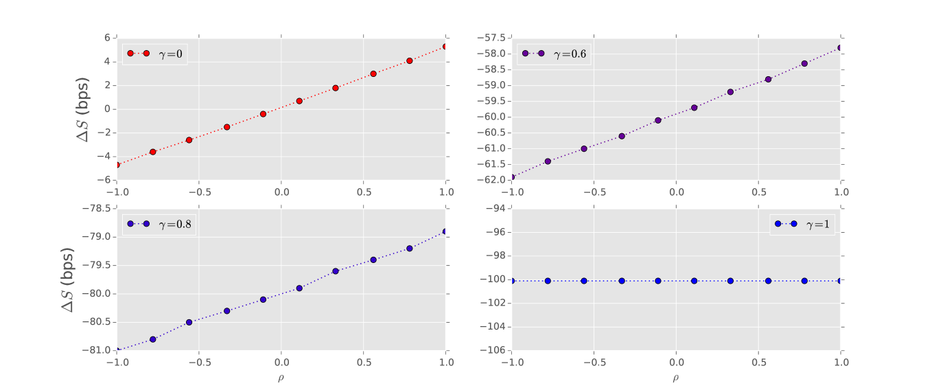
Figure 3: 5Y CDS par–spread impact vs $\rho$ and $\gamma$. The reference value for the par–spread is calculated using the parameters’ values in Table 2.

$z$		$\mu$		$\sigma^{Z}$		$a$		$b$		$y$		$\sigma^{Y}$		$T$
0.	8	0.	0	0.	1	0.	0001	-210.	0	-4.	089	0.	2	5.	0

Table 2: Parameters used to produce the par–spreads impact in Figure 3

Figure 4 shows that par–spreads’ sensitivity to the volatility of the FX rate process is slightly weaker than the one to the log-hazard rate’s volatility for the chosen ranges of parameters’ values. In our example, a 5Y par–spread can change of around 10 bps with $\sigma^{Z}$ ranging from 1% to 20%, while it can range up to 30 bps with $\sigma^{Y}$ going from 20% to 70% and with $\sigma^{Z}$ fixed at 20%.

figure[]

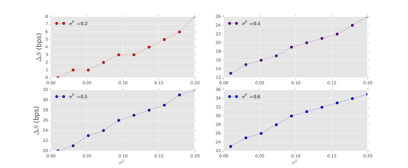
Figure 4: 5Y CDS par–spread impact vs $\sigma^{Z}$ and $\sigma^{Y}$. The reference value is produced using the parameters’ values in Table 3.

$z$		$\mu$		$\rho$		$a$		$b$		$y$		$T$
0.	8	0.	0	0.	5	0.	0001	-210.	0	-4.	089	5.	0

Table 3: Parameters used to produce the results shown in Figure 4.

In Figure 5 we show the sensitivity of par–spreads to the value of diffusive correlation $\rho$. The dependence of par spreads on the correlation is extremely weak for values of $\sigma^{Y}$ in the range of 20%. Around this level of log-hazard rate volatility, the maximum change that correlation can produce on the quanto-par spreads is 10 bps. From Figure 5, a more realistic value of $\sigma^{Y}$ of 60% is required to observe an impact of around 30 bps on the 5Y par–spread when changing the correlation from $-1$ to 1, showing the limits of a purely diffusive correlation model in explaining large differences between domestic and quanto-corrected CDS par-spreads.

figure[]

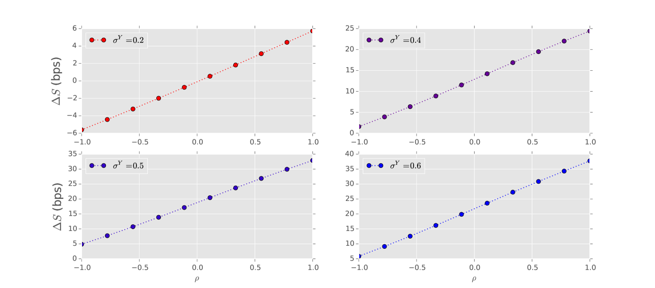
Figure 5: 5 years par–spread impact vs $\rho$ and $\sigma^{Y}$. The reference value is produced using the parameters’ values in Table 4.

$z$		$\mu$		$\sigma^{Z}$		$a$		$b$		$y$		$T$
0.	8	0.	0	0.	1	0.	0001	204.	0	-4.	089	5.	0

Table 4: Parameters used to produce the results shown in Figure 5.

There are circumstances where the basis between par–spreads of CDSs in different currencies can be sensibly higher than these values. In those cases, a purely diffusive model for the hazard rate is not sufficient to explain the observed basis and an approach where dependence is induced by devaluation jumps is required. As an example of an historical occurrence of such a wide basis, we show in Section 3.5 results of model calibrations to the time series of par–spreads for EUR-denominated and USD-denominated 5Y CDSs on the Italian Republic.

In the different context of impact of dependence on CDS credit valuation adjustments, even under collateralization, Brigo et al Brigo and Chourdakis (2009); Brigo et al. (2014, 2013) show that a copula function on the jump to default exponential thresholds may be necessary to obtain sizable effects when looking at credit–credit dependence, pure diffusive correlation not being enough.

3.3 Test on the Impact of Tenor and Credit Worthiness on the Quanto Correction

To test the relation given in Eq (73), we set the diffusive correlation to zero and we chose the following set of log-hazard rate parameters:

$$a =1.00e-004, b =-210.45 \sigma =0.2,$$

whereas we have produced low spread scenarios and high spread scenarios by choosing two different values for $Y_{0}$, the first one, $y^{L}=-4.089$, such that the resulting CDS par spread term structure is flat at around 100 bps, and the second one, $y^{H}=-2.089$ such to produce a flat CDS par spread term structure with a value of around 740 bps.

Figures 7 and 7 show, in line with the nature of the approximation (73), that the approximation is less accurate for higher maturities, as evident in both charts by comparing blue lines (short maturities) with red lines (long maturities). It is also less accurate and for higher values of CDS spreads, as highlighted by the comparison between Figure 7 (high spreads) and Figure 7 (low spreads).

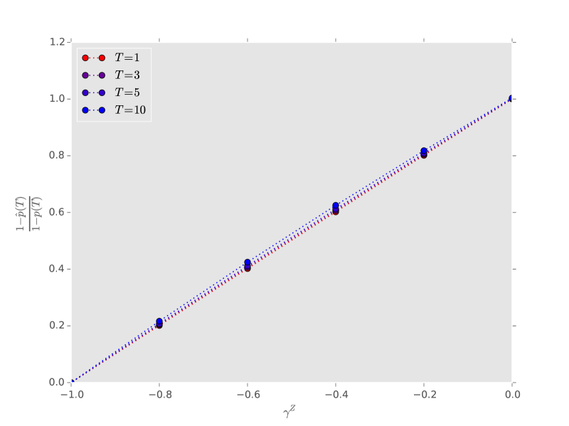
figure[.5] figure[.5]

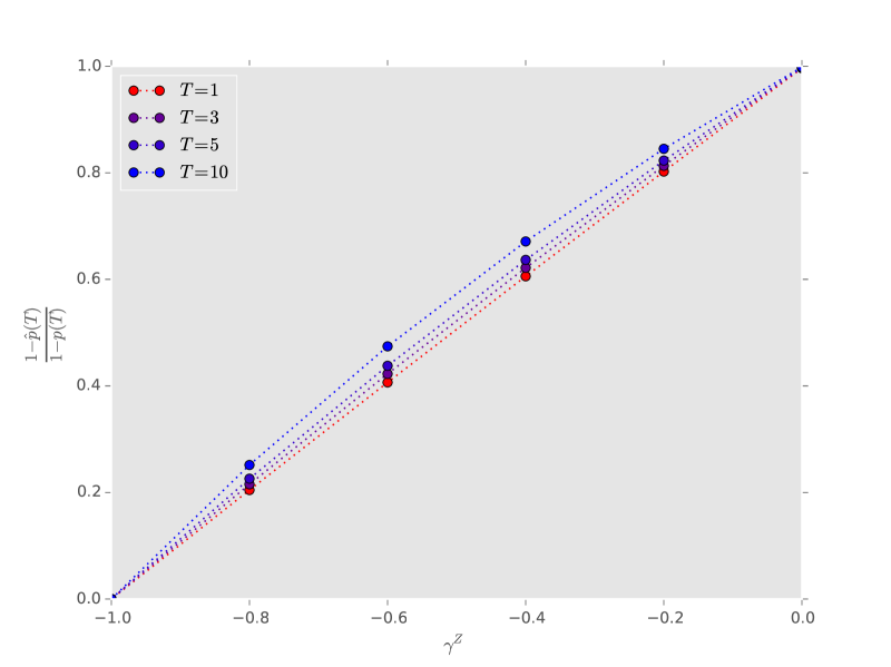
Figure 6: Comparison of curves $\nicefrac{{1-\hat{P}_{0}(T)}}{{1-P_{0}(T)}}$ for different maturities in a low spreads scenario, $Y_{0}=y^{L}$.

Figure 7: Comparison of $\nicefrac{{1-\hat{P}_{0}(T)}}{{1-P_{0}(T)}}$ for different maturities in a high spreads scenario, $Y_{0}=y^{H}$.

3.4 Correlation Impact on the Short Term Versus Long Term

We checked numerically the robustness of the theoretical relation between survival probabilities and $\gamma^{Z}$ that was shown in Eq (73). We calculated the ratio between the local and the quanto-corrected survival probability returned by the exponential OU model for different maturities and for different values of $\rho$. Furthermore, we express this value as a function of $\gamma^{Z}$, we call it $\hat{q}(\gamma)$, and we check how this value is affected by changes in $\gamma$. We then compare $\hat{q}$ with the limit-case value provided by Eq (73)

$$q(\gamma)\mathrel{\mathop{\mathchar 58\relax}}=1+\gamma.$$ (74)

The results, in the form of a percentage difference $\nicefrac{{q}}{{\hat{q}}}-1$, are reported in Table 5.

		$T=1$							$T=4$							$T=10$
$\gamma$		$\rho=-0.9$		$\rho=0$		$\rho=0.9$			$\rho=-0.9$		$\rho=0$		$\rho=0.9$			$\rho=-0.9$		$\rho=0$		$\rho=0.9$
-0.	99	0.	24 %	0.	08 %	$-0$.	07 %		$-2$.	60 %	$-3$.	33 %	$-4$.	05 %		$-31$.	74 %	$-34$.	93 %	-35.	58 %
-0.	50	0.	43 %	0.	28 %	0.	12 %		$-0$.	15 %	$-0$.	89 %	$-1$.	62 %		$-30$.	33 %	$-26$.	68 %	$-25$.	72 %
-0.	25	0.	53 %	0.	37 %	0.	22 %		1.	11 %	0.	37 %	$-0$.	36 %		$-15$.	84 %	$-15$.	01 %	$-14$.	87 %
0.	00	0.	63 %	0.	47 %	0.	31 %		2.	38 %	1.	65 %	0.	91 %		-1.	16 %	$-1$.	26 %	$-1$.	37 %
0.	25	0.	73 %	0.	57 %	0.	41 %		3.	67 %	2.	93 %	2.	20 %		13.	47 %	13.	71 %	14.	60 %
0.	50	0.	83 %	0.	67 %	0.	51 %		4.	96 %	4.	23 %	3.	50 %		28.	04 %	29.	82 %	35.	40 %

Table 5: Deviation from the relation in (73) expressed as percentage error between $1+\gamma$ and $\hat{q}(\gamma)$.

They show, as hinted in EL-Mohammadi (2009), that correlation has a smaller impact on short term survival probabilities: moving the correlation between the values of $-0.9$ and $0.9$ has an absolute impact of 0.3% on our results for 1Y survival probabilities, whereas the impact for 4Y survival probabilities is 1.45% and for 10Y survival probabilities is almost 4%. It has to be noted that for 10Y survival probabilities, $\hat{q}$ doesn’t provide a good approximation of $q$ not even in case of null correlation. This last fact is in line with the discussion carried out in Section 2.5.6, as in this case the hypotheses under which the approximation was deduced are not valid.

3.5 Model Calibration to Market Data for 2011–2013

In this section we present the results of the calibration of the model described in Section 2.5.5, where pricing currency and liquid currency coincide and are USD, and where we considered two contractual currencies, EUR and USD.

We used the observed CDSs spreads on Italy, both the USD-denominated ones and the EUR-denominated ones, to calibrate the model parameters. In principle, also single-name CDS swaptions could be used in this calibration process (see Brigo and Alfonsi (2005)), but, given the lack of liquidity on this instrument, we preferred proxying them with the at-the-money implied volatilities quoted for options on iTraxx Main.

3.5.1 Market Data Description

We calibrated the model to the market data for the three years using the time range 2011-2013. Let $\mathcal{T}=\{t_{0}\dots,t_{N}\}$ denote the dates in this sample period. We made the following assumptions on the market data:

1. we consider the CDS par–spreads on Republic of Italy with 5 years and 10 years tenor, both in USD and in EUR;

2. we use the same short rate for domestic and foreign currency

   $$r(t_{i})=\hat{r}(t_{i})=r,\quad t_{i}\in\mathcal{T},$$ (75)

3. on every $t_{i}\in\mathcal{T}$ we assign the value of the at–the–money Black–volatility from an option with 6 months expiry to $\sigma^{Z}$;

4. we keep the speed of mean reversion $a$ of $(Y_{t},t\geq 0)$ flat at the level $0.0001$;

5. on every $t_{i}\in\mathcal{T}$ we calibrated $\sigma^{Y}$ to the at-the-money option Black volatility for expiry one month.

Denoting by $p^{Y}\mathrel{\mathop{\mathchar 58\relax}}=(b,y_{0})$ the parameters to be calibrated for $(Y_{t},t\geq 0)$ that are needed in single currency CDS pricing, and by $p\mathrel{\mathop{\mathchar 58\relax}}=(b,y_{0},\rho,\gamma)$ the set of parameters needed to price a quanto CDS, we adopted the following procedure to calibrate the model in Eq (65)–(67):

1. first we calibrated $p^{Y}$ to the USD-denominated par–spread for the given date. We kept the parameters $a$ and $\sigma^{Y}$ fixed at a level of $0.0001$ and 50% respectively;

2. we calibrated $\sigma^{Y}$ to the CDS index option, keeping the $p^{Y}$ at the level calibrated at the previous step;

3. we used the calibrated value of $p^{Y}$ as a starting point in the iterative routine carried out to calibrate the set of model parameters $p$ to both the EUR-denominated and the USD-denominated CDSs. The starting guess point to calibrate $p$ can be written in terms of the calibrated point $p^{Y}$ as $p_{0}=(p^{Y}_{1},p^{Y}_{2},\gamma_{0},\rho_{0})$, where $\gamma_{0}$ and $\rho_{0}$ are the guess values for $\gamma$ and $\rho$. We kept $\sigma^{Y}$ fixed at the level calibrated at the previous step.

3.5.2 Results

In this section we show the results of the repeated daily calibrations to the 3 years of data contained in $\mathcal{T}$. The calibrated $\gamma$ and $\rho$ are showed in Figure 8 together with the relevant market data used in calibration, EUR-denominated and USD-denominated CDS par spreads for 5 years maturities, $S^{\textrm{{5}Y}}_{\textrm{EUR}}$ and $S^{\textrm{{5}Y}}_{\textrm{USD}}$, and for 10 years maturities, $S^{\textrm{{10}Y}}_{\textrm{EUR}}$ and $S^{\textrm{{10}Y}}_{\textrm{USD}}$ .

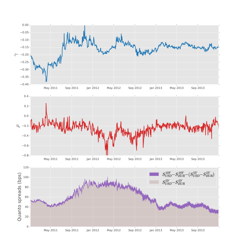
Figure 8: The top chart shows the calibrated $\gamma$ throught $\mathcal{T}$. The middle chart shows the calibrated $\rho$ thorught $\mathcal{T}$. The bottom chart shows the time series of corresponding quanto CDS par–spreads.

The aim of this section is to interpret the calibrated parameters in terms of market data. To do so, we will be relying on the theoretical results from the previous section.

Interpretation of the Devaluation Factor $\gamma^{Z}$

For the devaluation rate, $\gamma^{Z}$, we exploited the results from Section 2.5.6, and we used the relative basis spreads as an approximation

$$\gamma^{Z}\approx\frac{S_{\textrm{EUR}}-S_{\textrm{USD}}}{S_{\textrm{USD}}}.$$ (76)

As shown in Proposition 3, the simplified relation between $\gamma^{Z}$ and the ratio of the quanto and non–quanto corrected default probabilities is true for small values of the quantity $\int_{t}^{T}\lambda_{s}\operatorname{d\!}s$ so, since we could not control the credit quality in backtest, we relied on the time–to–maturity $T-t$ to achieve a good approximation. However, due to liquidity reasons, we used CDS par–spreads with 5 years and 10 years tenor, and these maturity values can be too large. Therefore we used model–implied par–spreads for this test; in this way we have been able to use also short maturities, like 1 year, that are usually not very liquid in the market.

The comparison between $\gamma^{Z}$ and its market-data approximation is showed in Figure 9. The left-hand chart, where 1Y-spreads have been used to build the relative basis spread, shows a surprisingly good agreement between the two variables. The same agreement does not hold for the right-hand chart, where 5Y-spreads were instead used. This is in line with the result of Proposition 3, that was derived under a limit hypothesis of short maturities.

It is worth highlighting that the approximation provided by Eq (76) would be an exact relation between $\gamma^{Z}$, $S_{\textrm{EUR}}$, and $S_{\textrm{USD}}$ for contracts for which it is possible to approximate the stream of the premium leg’s quarterly-spaced cash-flows with a continuously compounded stream of payments and in a setting where either the hazard rate was modeled as a deterministic function of time and where the CDS par–spread term structure was flat or in a setting where the hazard rate was modeled as a constant.

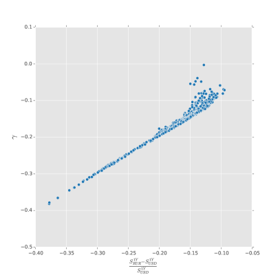
(a) Relative basis spread for 1Y maturity CDSs.

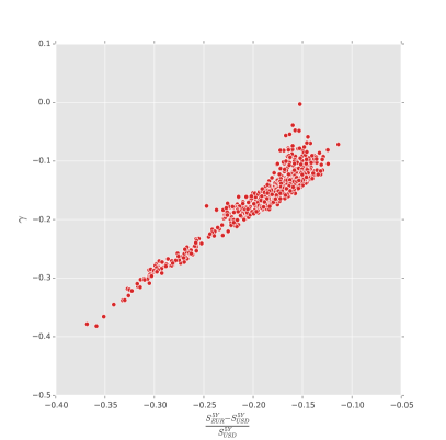
(b) Relative basis spread for 5Y maturity CDSs.

Figure 9: Scatter plot comparing the calibrated $\gamma^{Z}$ in ordinates with a relative basis spread in abscissas. As discussed in Section 3.5.2, the chart shows that the relative basis spread is a good estimate of the devaluation rate if the spreads have short maturities

Interpretation of the Instantaneous Correlation Parameter $\rho$

In order to provide a similar assessment on the parameter $\rho$, we relied on some heuristic results derived in Elizalde et al. (2010). In that technical report, a simplified pricing formula based on cost of hedging arguments is presented for quanto CDS . Their result can be written in terms of the variable defined by our framework as

$$\frac{S_{\textrm{EUR}}(T)-S_{\textrm{USD}}(T)}{S_{\textrm{USD}}(T)}\approx{\gamma^{Z}}+\sigma^{Y}\sigma^{Z}\rho\operatorname{RPV01}(T),$$ (77)

where $\operatorname{RPV01}(t)$ is the risky annuity of a CDS with tenor $t$ years. We applied the formula above to two tenor points $T_{1}$ and $T_{2}$ obtaining two equations, one for each tenor. In order to test the values of $\rho$ that we obtained in calibration, we worked out a single equation as a difference between the equations for the two tenor points:

$$\frac{S_{\textrm{EUR}}(T_{2})-S_{\textrm{USD}}(T_{2})}{S_{\textrm{USD}}(T_{2})}-\frac{S_{\textrm{EUR}}(T_{1})-S_{\textrm{USD}}(T_{1})}{S_{\textrm{USD}}(T_{1})}\approx\sigma^{Y}\sigma^{Z}\rho\left(\operatorname{RPV01}(T_{2})-\operatorname{RPV01}(T_{1})\right).$$ (78)

Specifically, we chose $T_{1}=1$, $T_{2}=10$ and we used the model–implied values of $S_{\textrm{EUR}}(T_{1})$, $S_{\textrm{EUR}}(T_{2})$, $S_{\textrm{USD}}(T_{1})$, $S_{\textrm{USD}}(T_{2})$, $\operatorname{RPV01}(T_{1})$ and $\operatorname{RPV01}(T_{2})$. We further used the values $\sigma^{Z}$ coming from the market while the values of $\sigma^{Y}$ and $\rho$ are the ones obtained in calibration ad discussed in Section 3.5.1. The results are presented in Figure 10 and they show a scatterplot of the proposed relation between model parameters and market data. The data are reported for the whole time–range 2011–2013 in Figure 10a, while Figure 10b contains the year–by–year plot. Due to the empirical nature of the Eq (78), we didn’t expect to find an exact relation between $\rho$ and other model parameters and market data. Nonetheless, a clear pattern is exhibited and this gives some confidence that such relation can be used to produce at least rough approximations for $\rho$ by using observable market data.

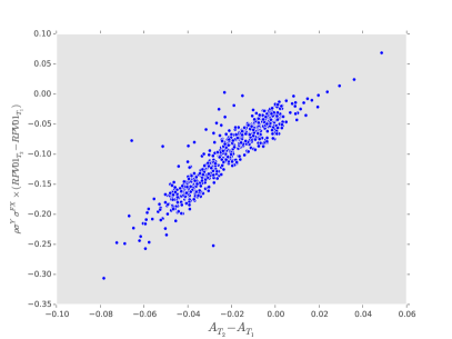
(a) Scatter plot for the time–range 2011–2013

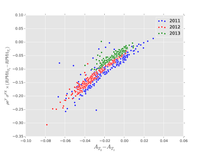
(b) Split by year

Figure 10: Scatter plot comparing the product of the calibrated $\rho$, $\sigma^{Y}$,$\sigma^{Z}$ and the model–implied difference between risky annuities in ordinates with a difference of relative basis spread in abscissas (we used $A_{T}\mathrel{\mathop{\mathchar 58\relax}}=\frac{S_{\textrm{EUR}}(T)-S_{\textrm{USD}}(T)}{S_{\textrm{USD}}(T)}$).

Model–Implied vs Historical Correlation

In Figure 11 we reported a comparison between the correlation parameter we obtained in calibration, $\rho$, and a historical estimator of correlation between daily log-returns of CDS par–spreads for one–year tenor contracts and daily log–returns of the FX spot rate. For assets where the market correctly prices gamma and cross–gamma risks, the basis between implied and realised covariance terms can be actually traded. This happens, for example, for implied and historical volatilities on equity indices.

In times where the values of implied and realised covariance terms diverge, the effect of such trading strategies is usually to bring them closer. We interpret the lack of evident convergence between implied and realised correlation in the chart in Figure 11 as a signal of the lack of an efficient market for this correlation risk.

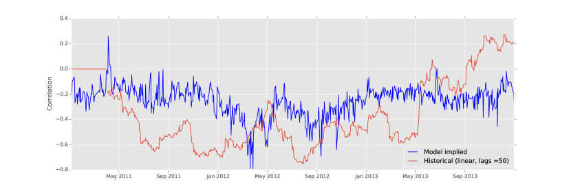
Figure 11: Implied and historical correlation between EURUSD FX rate and Italy’s CDS spread.

The fact that the implied correlation is generally smaller in absolute value than the realised one is consistent with our modeling choices and with the estimator used to calculate the realised correlation. The historical correlation has been estimated on a 50 days time–window using log–returns of the FX rate and this would neglect the impact of the jump term on its instantaneous volatility. Such an underestimation of the instantaneous volatility of the jump–diffusion process used in our modelling approach would result in an overestimation of the correlation with the credit component.

4 Conclusions and Further Work

We analysed default–driven FX devaluation jumps as a modelling mechanism. These can be used to explain the basis in credit default swaps offering protection on the same entity but in different currencies. We studied the case of Italy and EUR vs USD protection in particular. We found that the jump mechanism allows one to explain the size of the basis, whereas pure shock correlation between FX rates and credit spread is not sufficient. Further applications we may consider in future work include wrong–way risk modelling in credit valuation adjustment (CVA) applications.

Appendix A Proof of Proposition 2

Proof.

The relation between $Z$ and $X$ is given by $X_{t}=\phi(Z_{t})$ where $\phi(x)=1/x$. From Ito (see, for example, Jeanblanc et al. (2009))

$$\operatorname{d\!}X_{t} =\operatorname{d\!}\phi(Z_{t})=\phi^{\prime}(Z_{t-})\operatorname{d\!}Z_{t}+\frac{1}{2}\phi^{\prime\prime}(Z_{t-})\operatorname{d\!}\ [Z]^{c}_{t}+\sum_{s\leq t}\left(\left(\phi(Z_{s-}+\Delta Z_{s-})-\phi(Z_{s-})\right)-\phi(Z_{s-}){\Delta Z_{s-}}\right)$$

$$=\operatorname{d\!}\left(\frac{1}{Z_{t}}\right)=-\frac{\operatorname{d\!}Z_{t}}{Z_{t}^{2}}+\frac{\operatorname{d\!}\ [Z]^{c}_{t}}{Z_{t}^{3}}+\left(\frac{1}{Z_{t-}+\gamma^{Z}Z_{t-}}-\frac{1}{Z_{t-}}\right)\operatorname{d\!}D_{t}+\frac{\Delta Z}{Z_{t}^{2}}$$

$$=-\bar{\mu}\frac{1}{Z_{t}}\operatorname{d\!}t-\sigma^{Z}\frac{1}{Z_{t}}\operatorname{d\!}W_{t}^{(2)}-\gamma^{Z}\frac{1}{Z_{t-}}\operatorname{d\!}D_{t}+(\sigma^{Z})^{2}\frac{1}{Z_{t}}\operatorname{d\!}t+\frac{1}{Z_{t-}}\left(\frac{1}{1+\gamma^{Z}}-1\right)\operatorname{d\!}D_{t}+\frac{\gamma^{Z}}{Z_{t-}}\operatorname{d\!}D_{t}$$

$$=-\bar{\mu}\frac{1}{Z_{t}}\operatorname{d\!}t-\sigma^{Z}\frac{1}{Z_{t}}\operatorname{d\!}W_{t}^{(2)}+(\sigma^{Z})^{2}\frac{1}{Z_{t}}\operatorname{d\!}t+\frac{1}{Z_{t-}}\gamma^{X}\operatorname{d\!}D_{t}$$

$$=-\bar{\mu}X_{t}\operatorname{d\!}t-\sigma^{Z}X_{t}\operatorname{d\!}W_{t}^{(2)}+(\sigma^{Z})^{2}X_{t}\operatorname{d\!}t+X_{t-}\gamma^{X}\operatorname{d\!}D_{t}$$ (79)

where we used $\gamma^{X}$ to denote the jumps of $(X_{t},t\geq 0)$, given by

$$\gamma^{X}=-\frac{\gamma^{Z}}{1+\gamma^{Z}}.$$ (80)

We can now use Girsanov’s Theorem in the form of Eq 53a for $(W^{(2)}_{t},t\geq 0)$ and Eq 55 for $(D_{t},t\geq 0)$ to decompose $(X_{t},t\geq 0)$ in a sum of local martingales in the new measure $\hat{\mathbb{Q}}$. As a result

$$\operatorname{d\!}X_{t} =-\bar{\mu}X_{t}\operatorname{d\!}t-\sigma^{Z}X_{t}(\operatorname{d\!}\hat{W}_{t}^{(2)}-\sigma^{Z}\operatorname{d\!}t)+(\sigma^{Z})^{2}X_{t}\operatorname{d\!}t+X_{t-}\gamma^{X}(\operatorname{d\!}\hat{M}_{t}+(1+\gamma^{Z})(1-D_{t})\lambda_{t}\operatorname{d\!}t)$$

$$=-(\bar{\mu}-\gamma^{X}(1+\gamma^{Z})(1-D_{t})\lambda_{t}\operatorname{d\!}t)X_{t}\operatorname{d\!}t-\sigma^{Z}X_{t}\operatorname{d\!}\hat{W}_{t}^{(2)}+X_{t-}\gamma^{X}\operatorname{d\!}M_{t}$$ (81)

Reminding that $\bar{\mu}$ is given by (see Eq (16) and (61)) $r-\hat{r}-(1-D_{t})\gamma^{Z}\lambda_{t}$, the $\mathbb{Q}$-dynamics of $(Z_{t},t\geq 0)$ can be written as

$$\operatorname{d\!}X_{t} =(\hat{r}-r+\gamma^{Z}(1-D)\lambda_{t}+\gamma^{X}(1+\gamma^{Z})(1-D_{t})\lambda_{t})X_{t}\operatorname{d\!}t-\sigma^{Z}X_{t}\operatorname{d\!}\hat{W}_{t}^{(2)}+X_{t-}\gamma^{X}\operatorname{d\!}\hat{M}_{t}$$

$$=(\hat{r}-r)X_{t}\operatorname{d\!}t-\sigma^{Z}X_{t}\operatorname{d\!}\hat{W}_{t}^{(2)}+X_{t-}\gamma^{X}\operatorname{d\!}\hat{M}_{t}.$$ (82)

∎

Appendix B Proof of Proposition 3

Proof.

Using Bayes’ formula we can write

$$\mathbb{E}_{t}\left[Z_{T}\mathbbm{1}_{\tau>T}\right]=\mathbb{E}_{t}\left[Z_{T}|\ \mathbbm{1}_{\tau>T}\right]\mathbb{E}_{t}\left[\mathbbm{1}_{\tau>T}\right]$$

Under the dynamics given by (51), the FX rate has only one jump at the default time of the reference entity, therefore it is subject to no jumps conditioned to the event $\mathbbm{1}_{\tau>T}$. This fact, together with the independence between the Brownian motions driving the FX and the hazard rate processes, allows to write:

$$\mathbb{E}_{t}\left[Z_{T}|\ \mathbbm{1}_{\tau>T}\right]=Z_{0}\mathbb{E}_{t}\left[e^{\mu(T-t)-\gamma^{Z}\int_{t}^{T}\lambda_{s}\operatorname{d\!}s}\right]=Z_{0}e^{\mu(T-t)}\mathbb{E}_{t}\left[e^{-\gamma^{Z}\int_{t}^{T}\lambda_{s}\operatorname{d\!}s}\right]$$

so that the survival probabilities are linked by

$$\hat{p}_{t}(T)=\frac{\mathbb{E}_{t}\left[Z_{T}\mathbbm{1}_{\tau>T}\right]}{Z_{t}}\frac{B(t,T)}{\hat{B}(t,T)}=\mathbb{E}_{t}\left[e^{-\gamma^{Z}\int_{t}^{T}\lambda_{s}\operatorname{d\!}s}\right]p_{t}(T).$$

The above can be written in terms of default probabilities,

$$1-\hat{p}_{t}(T)=1-\mathbb{E}_{t}\left[e^{-\gamma^{Z}\int_{t}^{T}\lambda_{s}\operatorname{d\!}s}\right]p_{t}(T)=1-p_{t}(T)+\left(1-\mathbb{E}_{t}\left[e^{-\gamma^{Z}\int_{t}^{T}\lambda_{s}\operatorname{d\!}s}\right]\right)p_{t}(T),$$

so that the ratio of default probabilities can be expressed as

$$\frac{1-\hat{p}_{t}(T)}{1-p_{t}(T)} =1+\left(1-\mathbb{E}_{t}\left[e^{-\gamma^{Z}\int_{t}^{T}\lambda_{s}\operatorname{d\!}s}\right]\right)\frac{p_{t}(T)}{1-p_{t}(T)}$$

$$=1+\left(1-\mathbb{E}_{t}\left[e^{-\gamma^{Z}\int_{t}^{T}\lambda_{s}\operatorname{d\!}s}\right]\right)\frac{\mathbb{E}_{t}\left[e^{-\int_{t}^{T}\lambda_{s}\operatorname{d\!}s}\right]}{1-\mathbb{E}_{t}\left[e^{-\int_{t}^{T}\lambda_{s}\operatorname{d\!}s}\right]}.$$ (83)

Given that our aim is to find an approximation for small maturities, it is convenient to note that

$$e^{-\int_{0}^{T}\lambda_{s}\operatorname{d\!}s}=1-\lambda_{0}T+O(T^{2})\quad\mbox{as }T\rightarrow 0$$ (84)

so that we can write the right hand side of Eq (B) at $t=0$ as

rhs Eq (B) $$=1+\left(1-\mathbb{E}_{0}\left[1-\gamma^{Z}\lambda_{0}T+O(T^{2})\right]\right)\frac{\mathbb{E}_{0}\left[1-\lambda_{0}T+O(T^{2})\right]}{\mathbb{E}_{0}\left[\lambda_{0}T+O(T^{2})\right]}$$

$$=1+\gamma^{Z}({\lambda_{0}T+\mathbb{E}_{0}[O(T^{2})]})\frac{{1-\lambda_{0}T+\mathbb{E}_{0}[O(T^{2})]}}{{\lambda_{0}T+\mathbb{E}_{0}[O(T^{2})]}}$$

$$=1+\gamma^{Z}(1-\lambda_{0}T+\mathbb{E}_{0}[O(T^{2})])\frac{\lambda_{0}T}{{\lambda_{0}T+\mathbb{E}_{0}[O(T^{2})]}}+\gamma^{Z}{\mathbb{E}_{0}[O(T^{2})]}\frac{{1-\lambda_{0}T+\mathbb{E}_{0}[O(T^{2})}}{{\lambda_{0}T+\mathbb{E}_{0}[O(T^{2})]}}$$

$$=1+\gamma^{Z}(1-\lambda_{0}T+\mathbb{E}_{0}[O(T^{2})])\frac{1}{1+\frac{\mathbb{E}_{0}[O(T^{2})]}{\lambda_{0}T}}+\gamma^{Z}{\mathbb{E}_{0}[O(T^{2})]}\frac{{1-\lambda_{0}T+\mathbb{E}_{0}[O(T^{2})]}}{{\lambda_{0}T+\mathbb{E}_{0}[O(T^{2})]}}$$

from which we have

$$\frac{1-\hat{p}_{0}(T)}{1-p_{0}(T)}\rightarrow 1+\gamma^{Z},\quad\mbox{as }T\rightarrow 0.$$ (85)

∎

Disclaimers

The opinions and views are uniquely those of the authors and do not necessarily represent those of their employers.

References

- Bielecki et al. [2008] R. T. Bielecki, M. Jeanblanc, and M. Rutkowski. Pricing and Trading Credit Default Swaps in a Hazard Process Model. Annals of Applied Probability, 18(6):2495–2529, 2008.
- Bielecki et al. [2005] T. R. Bielecki, M. Jeanblanc, and M. Rutkowski. PDE approach to valuation and hedging of credit derivatives. Quantitative Finance, 5, 2005.
- Biffis et al. [2016] E. Biffis, D. Blake, L. Pitotti, and A.J. Sun. The Cost of Counterparty Risk and Collateralization in Longetivity Swaps. Journal of Risk and Insurance, 83:387–419, 2016.
- Brigo and Alfonsi [2005] D. Brigo and A. Alfonsi. Credit Default Swap Calibration and Derivatives Pricing with the SSRD Stochastic Intensity Model. Finance and Stochastic, 9(1):29–42, 2005.
- Brigo and Chourdakis [2009] D. Brigo and K. Chourdakis. Counterparty Risk for Credit Default Swaps: Impact of Spread Volatility and Default Correlation. International Journal of Theoretical and Applied Finance, 12(07):1007–1026, 2009.
- Brigo and El-Bachir [2010] D. Brigo and N. El-Bachir. An exact formula for default swaptions’ pricing in the SSRJD stochastic intensity model. Mathematical Finance, 20:365–382, July 2010.
- Brigo and Mercurio [2006] D. Brigo and F. Mercurio. Interest Rate Models — Theory and Practice: With Smile, Inflation and Credit. Springer, second edition, 2006.
- Brigo et al. [2013] D. Brigo, M. Morini, and A. Pallavicini. Counterparty Credit Risk, Collateral and Funding: with pricing cases for all asset classes. Wiley, 2013.
- Brigo et al. [2014] D. Brigo, A. Capponi, and A. Pallavicini. Arbitrage–free bilateral counterparty risk valuation under collateralization and application to Credit Default Swaps. Mathematical Finance, 24(1):125–146, 2014.
- Cherubini [2005] U. Cherubini. Counterparty risk in derivatives and collateral policies: the replicating portoflio approach . Proceedings of the Counterparty Credit Risk 2005 CREDIT conference, pages 22–23, 2005.
- Cherubini et al. [2004] U. Cherubini, E. Luciano, and W. Vecchiato. Copula Methods in Finance. Wiley, 2004.
- During et al. [2013] B. During, M. Fournié, and A. Rigal. High Order ADI Schemes for convection–diffusion equations with mixed derivatives terms. Spectral and High Order Methods for Partial Differential Equations – ICOSAHOM’12, pages 217–226, 2013.
- Ehlers and Schönbucher [2006] P. Ehlers and P. Schönbucher. The Influence of FX Risk on Credit Spreads. Working Paper, ETH, 2006.
- EL-Mohammadi [2009] R. EL-Mohammadi. BSFTD With Multi Jump Model And Pricing Of Quanto FTD With FX Devaluation Risk. Munich Personal RePEc Archive, 2009.
- Elizalde et al. [2010] A. Elizalde, S. Doctor, and H. Singh. Trading credit in different currencies via Quanto CDS. Technical report, J.P. Morgan, October 2010.
- Jeanblanc et al. [2009] M. Jeanblanc, M. Yor, and M. Chesney. Mathematical Methods for Financial Markets. Springer, 2009.
- Kim and Leung [2016] J. Kim and T. Leung. Pricing derivatives with counterparty risk and collateralization: A fixed point approach. European Journal of Operational Research, 249:525–539, 2016.
- Lando [2004] D. Lando. Credit Risk Modeling: Theory and Applications. Princeton University Press, 2004.
- Lorig et al. [2015] M. Lorig, S. Pagliarini, and A. Pascucci. A family of density expansions for Lévy–type processes. Annals of Applied Probability, 25(1):235–267, 2015.
- Pykthtin and Sokol [2013] Michael Pykthtin and Alexander Sokol. Exposure under systemic impact. Risk Magazine, pages 88–93, 2013.