Popularity Signals in Trial-Offer Markets
with Social Influence and Position Bias

Abstract

This paper considers trial-offer markets where consumer preferences are modeled by a multinomial logit with social influence and position bias. The social signal for a product is given by its current market share raised to power $r$ (or equivalently the number of purchases raised to the power of $r$). The paper shows that, when $r$ is strictly between 0 and 1, and a static position assignment (e.g., a quality ranking) is used, the market converges to a unique equilibrium where the market shares depend only on product quality, not their initial appeals or the early dynamics. When $r$ is greater than 1, the market becomes unpredictable. In many cases, the market goes to a monopoly for some product: Which product becomes a monopoly depends on the initial conditions of the market. These theoretical results are complemented by an agent-based simulation which indicates that convergence is fast when $r$ is between 0 and 1, and that the quality ranking dominates the well-known popularity ranking in terms of market efficiency. These results shed a new light on the role of social influence which is often blamed for unpredictability, inequalities, and inefficiencies in markets. In contrast, this paper shows that, with a proper social signal and position assignment for the products, the market becomes predictable, and inequalities and inefficiencies can be controlled appropriately.

Keywords. System dynamics, social influence, stochastic dynamics, Robbins-Monro algorithms, popularity signals, ranking policies.

1 Introduction

The impact of social influence and product visibilities on consumer behaviour in Trial-Offer (T-O) markets has been explored in a variety of settings (e.g., [26, 30, 33]). Social influence can be dispensed through different types of social signals: A market place may report the number of past purchases of a product, its consumer ratings, and/or its consumer recommendations. Recent studies [13, 33] however came to the conclusion that the popularity signal (i.e., the number of past purchases or the market share) has a much stronger impact on consumer behaviour than the average consumer rating signal. These two experimental studies were conducted in very different settings, using the Android application platform in one case and hotel selection in the other. Consumer preferences are also influenced by product visibilities, a phenomenon that has been widely observed in internet advertisement (e.g., [11]), in online stores such as Expedia, Amazon, and iTunes, as well as physical retail stores (see, e.g., [20]).

Despite its widespread use in online settings (including for songs, albums, movies, hotels, and cell phones to name only a few), there is considerable debate in the scientific community about the benefits of social influence. Many researchers have pointed out the potential negative effects of social influence. The seminal work of Salganik et al. [26] on the MusicLab experimental market demonstrated that social influence can introduce significant unpredictability, inequality, and inefficiency in T-O markets. These results were reproduced by many researchers (e.g.,  [28, 27, 23, 31]). More recently, Hu et al. [15] studied a newsvendor problem with two substitutable products with the same quality in which consumer preferences are affected by past purchases. The authors showed that the market is unpredictable but can become less so if one of products has an initial advantage. Altszyler et al. [5] has recently studied the impact of product appeal and product quality in a trial-offer market model with social influence under a finite time horizon. The authors showed that there exists a logarithmic tradeoff between the two: the final product market share remains constant if a decrease in product quality is followed by an exponential increase in the product appeal. Other researchers have focused on understanding when these undesirable side-effects arise and where they come from. Ceyhan et al. [8] studied a market specified by a logit model where a constant $J$ captures the strength of the social signal. They showed that the market behaviour (e.g., whether it is predictable) depends on the strength of the social signal. Their results did not consider product visibilities, which is another important aspect of T-O markets. Indeed, various researchers (e.g., [19, 1, 32, 3, 4]) indicated that unpredictability and inefficiencies often depend on how products are displayed in the market. In particular, Abeliuk et al. [1] show that social influence is always beneficial in expectation when the products are ordered by the performance ranking that maximises the purchases greedily at each step. This result was obtained using the generalised multinomial logit model proposed by Krumme et al. [17] to reproduce the MusicLab experiments. Van Hentenryck et al. [32] proves a similar result for the quality ranking that assigns the highest quality products to the most visible positions. In addition, they show that the market converges to a monopoly for the highest quality product. These results contrast with the MusicLab experiments which relied on the popularity ranking that dynamically assigns the most popular products to the most visible positions.

This paper seeks to expand our understanding of social influence in T-O markets and explores the role of the social signal in conjunction with product visibilities. Our starting point is the generalised multinomial logic model of Krumme et al. [17], which we extend to vary the strength of the social signal. More precisely, this paper considers a T-O market where the probability of purchasing product $i$ at time $t$ is given by

$$p_{i}(\phi^{t})=\frac{v_{\sigma(i)}q_{i}(\phi_{i}^{t})^{r}}{\sum_{j=1}^{n}v_{\sigma(j)}q_{j}(\phi_{j}^{t})^{r}}$$ (1)

where $\sigma$ is a bijection from $n$ products to $n$ positions, $v_{k}\in\mathbb{R}$ is the visibility of position $k$, $q_{i}\in\mathbb{R}$ is the inherent quality of product $i$, $\phi_{i}^{t}$ is the market share of product $i$ at time $t$, and $r>0$ is the strength of the social signal. As should be clear from the discussion above, prior work on T-O markets with product visibilities (e.g., [19, 1, 32, 3]) focused on the case of a linear social signal ($r=1$). The primary objective of this paper is to understand what happens to the T-O market when $r<1$.

The paper contains both theoretical and simulation results and its contributions can be summarised as follows:

1. When $r<1$ and a static ranking is used, the market converges to a unique equilibrium, which we characterise analytically. In the equilibrium, the market shares depend only on the product qualities $q_{i}$ and no monopoly occurs. Moreover, a product of higher quality receives a larger market share than a product of lower quality, introducing a notion of fairness in the market and reducing the inequalities introduced by a linear social signal.

2. When $r>1$ and a static ranking is used, the equilibria can be characterised similarly. However, contrary to the case $r<1$, the equilibria that are not monopolies can be shown to be unstable under certain conditions. As a result, the market will typically go to a monopoly for some product: Which product wins the entire market share depends on the initial condition and the early dynamics.

3. Agent-based simulations show that the market converges quickly towards an equilibrium when using sublinear social signals and the quality ranking. They also show that the quality ranking outperforms the popularity ranking in maximising the efficiency of the market. The popularity ranking is also shown to have some significant drawbacks in some settings.

These theoretical results indicate that, when the social influence signal is a sublinear function of the market share and a static ranking of the products (e.g., the quality ranking) is used, the market is entirely predictable, depends only on the product quality, and does not lead to a monopoly. This contrasts with the case of $r=1$ where the market is entirely predictable but goes to a monopoly for the product of highest quality (assuming the quality ranking) [32] and the case of $r>1$ where the market becomes unpredictable (even with a static ranking). As a result, sublinear social signals provide a way to balance market efficiency and the inequalities introduced by social influence. In particular, with sublinear social signals and a static ranking, markets do not exhibit a Matthew effect where the winner takes all, and remain predictable.

The remaining of this paper is organised as follows. Section 2 describes the related work. Section 3 introduces T-O markets and the generalised multinomial logit model for consumer preferences considered here. Section 4 reviews some necessary mathematical preliminaries, including the fact that T-O markets can be modeled as Robbins-Monro algorithms. Section 5 derives the equilibria for the market as a function of the social signal and also presents the convergence results. Section 6 reports the results from the agent-based simulation. Section 7 discusses some additional results on sublinear signals. Section 8 discusses the results and concludes the paper.

2 Related Work

The research presented in this paper was motivated by the seminal work of Salganik et al. [26]. They study an experimental market called the MusicLab, where participants were presented a list of unknown songs from unknown bands, each song being described by its name and band. The participants were partitioned into two groups exposed to two different experimental conditions: the independent condition and the social influence condition. In the independent group, participants were shown the songs in a random order and they were allowed to listen to a song and then to download it if they so wish. In the second group (social influence condition), participants were shown the songs in popularity order, i.e., by assigning the most popular songs to the most visible positions. Moreover, these participants were also shown a social signal given by the number of times each song was downloaded. In order to investigate the impact of social influence, participants in the second group were distributed in eight “worlds” evolving completely independently. In particular, participants in one world had no visibility about the downloads and the rankings in the other worlds. The MusicLab exemplifies a T-O market where each song represents a product, and listening and downloading a song represent trying and purchasing a product respectively. The results in [26] show that different worlds evolve differently from one another, and significantly so, providing evidence that social influence may introduce unpredictability, inequalities, and inefficiency in the market.

The results in [26] were reproduced by numerous researchers (e.g.,  [28, 27, 23, 31]) and, in particular, by Krumme et al. [17] who model the MusicLab experiment with a generalised multinomial logit where product utilities depend on the song appeal, quality, visibility, and a social influence signal representing past purchases. The T-O market studied in this paper generalises the model proposed by Krumme et al., exploring various strengths for the social signal as indicated in Equation 1. The case of a linear signal ($r=1$) has been given significant attention. Abeliuk et al [1] proposed the performance ranking which orders the products optimally at each time $t$ given the appeals, qualities, visibilities, and market shares. They show that, when the performance ranking is used, the market always benefits from social influence in expectation. Van Hentenryck et al. [32] study the quality ranking which ranks the products by quality: They show that the quality ranking and, more generally, any static ranking, always benefits from social influence in expectation. They also prove that the market converges almost surely to a monopoly for the highest-quality product, indicating that the quality ranking is both optimal and predictable asymptotically. These results extend well-known theorems on Pólya urns and their generalisations (e.g., [22, 9, 24]). Abeliuk et al. [3] also show that the performance ranking converges to a monopoly for the highest-quality product when a linear social signal is used.

Ceyhan et al. [8] study a general choice probability $C_{i}^{J}(\phi^{t})$, where $J$ represents the strength of the social signal, and prove some general convergence results under some assumptions. In particular, they use the ODE method [21] and a Lyapunov function (e.g., [18]) to prove that the market converges to an equilibrium when the Jacobian of $C_{i}^{J}$ is symmetric (which is not the case when product visibilities are present). They also study in detail the case where the market follows a logit model of the form

$$C_{i}^{J}(\phi)=\frac{e^{J\phi_{i}+q_{i}}}{\sum_{j}e^{J\phi_{j}+q_{j}}}$$

where $J$ is a constant capturing the strength of the social influence signal. They show that there exists a parameter $J^{*}$ such that the market converges toward a unique equilibrium when $J<J^{*}$ and to a monopoly when $J\geq J^{*}$. No analytical characterisation of the equilibrium when $J<J^{*}$ is presented.

It is interesting to contrast these and our results. Observe first that the proof technique used in [8] relies on the fact that the Jacobian of $C_{i}^{J}$ is symmetric, which is not the case for T-O markets with product visibilities. Our paper studies such T-O markets and show that, when $0<r<1$ and a static ranking is used, the market converges to an inner equilibrium, which we characterise analytically. When $r=1$, the T-O market converges to a monopoly for the product with the highest value $v_{\sigma(i)}q_{i}$ [1]. When $r>1$, we show that the equilibria of the T-O market are given by monopolies for each product and other type of equilibria (e.g, a market share consisting on a distribution $60\%,40\%,0\%$ for a market with 3 products). We prove that, when $r>1$, the equilibria that are not monopolies are unstable (under certain conditions). As a result, the market will likely converge to a monopoly for some product.

It is also useful to mention that different, theoretical and experimental, approaches to the use of social influence are present in the literature. For instance, Yuan and Hwarng [35] describe a demand-based pricing model under social influence and capture its behaviour with a dynamical system that evolve to some stable or chaotic equilibria depending on the strength of the social signal. Stummer et al [29] introduces an agent-based model for repeat purchase decisions addressing different types of innovation diffusion and their perceived attributes; They also applied this methodology to an application concerned with second-generation biofuel.

3 The Trial-Offer Model

The paper builds on the work by Krumme et al. [17] who propose a framework in which consumer choices are captured by a multinomial logit model whose product utilities depend on the product appeal, position bias, and a social influence signal representing past purchases. A marketplace consists of a set $N$ of $n$ items. Each item $i\in N$ is characterised by two values:

1. its appeal $a_{i}>0$ which represents the inherent preference of trying item $i$;

2. its quality $q_{i}>0$ which represents the conditional probability of purchasing item $i$ given that it was tried.

This paper assumes that the appeals and the qualities are known. Abeliuk et al. [1] have shown that these values can be recovered accurately and quickly, either before or during the market execution using the approximation suggested by Krumme et al.:

$$a_{i}\sim\frac{s_{i}}{\sum_{j}s_{j}}$$

and

$$q_{i}\sim\frac{d_{i}}{s_{i}}$$

where $s_{i}$ and $d_{i}$ are the samplings and purchases of product $i$ at some point in time.

The objective of the firm running this market is to maximise the total expected number of purchases. To achieve this, the key managerial decision of the firm is what is known as the ranking policy [1], which consists in deciding how to display the products in the market (e.g., where to display a product on a web page). Here we assume that, at the beginning of the market, the firm decides upon a ranking for the items, i.e., an assignment of items to positions in the marketplace. Each position $j$ has a visibility $v_{j}$ which represents the inherent probability of trying an item in position $j$. A ranking $\sigma$ is a permutation of the items and $\sigma(i)=j$ means that item $i$ is placed in position $j$ ($j\in N$). When a customer enters the market, she observes all the items and their social signals based on the values of the previous purchases $d^{t}=(d^{t}_{1},\ldots,d^{t}_{n})$.

The vector $\phi^{t}$ of market shares at time $t$ is computed in terms of the vector $d^{t}$, i.e.,

$$\phi_{i}^{t}=\frac{d_{i}^{t}}{\sum_{j=1}^{n}d_{j}^{t}}.$$

and

$$\phi^{t}\in\Delta^{n-1}=\{x=(x_{1},\ldots,x_{n})\in\mathbb{R}^{n}\ \mid\ 0\leq x_{i}\leq 1\mbox{ and }\sum_{i=1}^{n}x_{i}=1\}.$$

The consumer then selects an item to try. The probability that the customer tries item $i$ is given by $P_{i}(\sigma,\phi^{t})$ where

$$P_{i}(\sigma,\phi)=\frac{v_{\sigma(i)}f(\phi_{i})}{\sum_{j=1}^{n}v_{\sigma(j)}f(\phi_{j})}$$ (2)

and $f$ is a continuous, positive, and nondecreasing function. This probability generalises the multinomial logit model of Krumme et al. [17] who define two sets of probabilities, $p^{SI}_{i,t}$ and $p^{I}_{i}$, that capture the probability of trying product $i$ with and without social influence. These probabilities are defined as:

$$p^{SI}_{i,t}=\frac{v_{\sigma(i)}(\alpha a_{i}+d_{i}^{t})}{\sum_{j=1}^{n}v_{\sigma(j)}(\alpha a_{j}+d_{j}^{t})},\qquad p_{i}^{I}=\frac{v_{\sigma(i)}a_{i}}{\sum_{j=1}^{n}v_{\sigma(j)}a_{j}},$$ (3)

where $\alpha$ is a parameter to calibrate the strength of the social signal (e.g., $\alpha=200$ for the MusicLab experiments). Equation (2) allows us to recover the formulae (3) via some linear transformation of the identity function: $f(\phi_{i})=\beta\phi_{i}+\alpha a_{i},$ with $\beta=\sum_{j}d_{j}$ or $\beta=0$ for each case.

After having tried product $i$, a customer decides whether to buy the sampled item and the probability that she purchases item $i$ is given by $q_{i}$. If item $i$ is purchased at time $t$, then the purchase vector becomes

$$d_{j}^{t+1}=\left\{\begin{array}[]{ll}d_{j}^{t}+1&\mbox{ if }j=i;\\ d_{j}^{t}&\mbox{ otherwise.}\end{array}\right.$$

For simplicity, the vector $d^{0}$ is initialised with the product appeals, i.e., $d_{i}^{0}=a_{i}$. This condition can be relaxed and the results presented in this paper continue to hold but the notations are heavier (See Appendix C for the details). To analyse this process, we divide time into discrete periods such that each new period begins when a product has been purchased. Hence, the length of each time period is not constant.

In this paper, we are interested in characterising how the market shares $\{\phi^{t}\}_{t>0}$ evolve over time for various functions $f$ given a static ranking $\sigma$. We are particularly interested in study the asymptotic behaviour of $\{\phi^{t}\}_{t>0}$ for the cases where $f(x)=x^{r}$ with $r>0$. For instance, when $r=0.5$, the social signal displays the square root of the number of past purchases. For notational simplicity, we assume that the ranking is fixed and is the identity function $\sigma(i)=i$ and omit it from the formulas. If the qualities and visibilities also satisfy $q_{1}\geq\ldots\geq q_{n}$ and $v_{1}\geq\ldots\geq v_{n}$, we obtain the quality ranking proposed in [32] but our results hold for any static ranking.

The following lemma, whose proof is in Appendix B, relates the two phases of the T-O market and characterises the probability that the next purchase is item $i$. It generalises a result in [32].

Lemma 3.1.

If $f:[0,1]\to\mathbb{R}$ is a positive function, then the probability $p_{i}(\phi)$ that the next purchase is the product $i$ given the market share vector $\phi$ is given by

$$p_{i}(\phi)\ =\frac{v_{i}q_{i}f(\phi_{i})}{\sum_{j=1}^{n}v_{j}q_{j}f(\phi_{j})}.$$ (4)

We finish this section with an important equivalence that arises when $f(x)=x^{r}$, $r>0$. Under such condition, if one writes down Equation (4) in terms of the number of purchases $d_{i}$ that product $i$ has so far obtained instead of using the market shares, we get exactly the same expression. Indeed,

$$p_{i}(\phi)=\frac{v_{i}q_{i}(\phi_{i})^{r}}{\sum_{j}v_{j}q_{j}(\phi_{j})^{r}}=\frac{v_{i}q_{i}(\frac{d_{i}}{\sum_{k}d_{k}})^{r}}{\sum_{j}v_{j}q_{j}(\frac{d_{j}}{\sum_{k}d_{k}})^{r}}=\frac{v_{i}q_{i}(d_{i})^{r}}{\sum_{j}v_{j}q_{j}(d_{j})^{r}}.$$ (5)

Thus, when the social signal function $f$ is given by $f(x)=x^{r}$, $r>0$, it is possible to interpret our model either using the concept of market share (as we describe in Section 3) or simply using the current number of purchases.

4 Trial-Offer Markets as Robbins-Monro Algorithms

This section establish some basic definitions and concepts that are useful in the rest of the paper. In particular, it shows that T-O markets can be modeled as Robbins-Monro algorithms and states some useful results. The results in this section are well-known in stochastic approximation. The section starts with a brief introduction of Ordinary Differential Equations (ODE) and some stability criteria (e.g., see [14, 16]).

Differential Equations:

Consider the following differential equation

$$\frac{dy}{dt}=F(y)$$ (6)

where $F$ is some vector field. The concept of equilibrium is central in the study of asymptotic behaviour for this type of equation.

Definition 4.1.

A vector $y^{*}\in\mathbb{R}^{n}$ is an equilibrium for differential equation (6) if $F(y^{*})=0$.

We are interested in equilibria that satisfy (at least) certain stability criteria.

Definition 4.2.

An equilibrium $y^{*}$ is said to be stable for Equation (6) if, given $\epsilon>0$, there exists $\delta>0$ such that $\|y(t)-y^{*}\|<\epsilon$ for all $t>0$ and for all $y$ such that $\|y-y^{*}\|<\delta$. We say that $y^{*}$ is asymptotically stable if it also satisfies

$$\lim_{t\to\infty}y(t)=y^{*}.$$

Remark 4.3.

When an equilibrium $y^{*}$ is not stable, we say that $y^{*}$ is unstable.

The asymptotic stability of an equilibrium $y^{*}$ can be characterised in terms of the Jacobian matrix $JF(y^{*})=(\frac{\partial F_{i}(y^{*})}{\partial y_{j}})_{i,j}$ $(i,j\in N)$ as stated by the following Theorem (see, for instance, [16] p. 440).

Theorem 4.4.

Let $y^{*}$ be an equilibrium for the differential equation (6). If the eigenvalues of the Jacobian matrix $JF(y^{*})$ all have negative real part, then $y^{*}$ is asymptotically stable. If, on the other hand, $JF(y^{*})$ has at least one eigenvalue with a positive real part, then $y^{*}$ is unstable.

A well-known result from linear algebra (see, for example, [25] p. 296) establishes the connection between the trace of a square matrix and its eigenvalues. In the following, we use $tr(A)=\sum_{i}^{n}a_{ii}$ to denote the trace of matrix $A$ where $a_{ii}$ are the diagonal entries of matrix $A$.

Theorem 4.5.

Let $A$ be a $n\times n$ matrix, and $\lambda_{1},...,\lambda_{n}$ its eigenvalues. Then $tr(A)=\sum_{i=1}^{n}\lambda_{i}$.

We now show that the discrete stochastic process $\{\phi^{t}\}_{t\geq 0}$ can be modeled as a Robbins-Monro Algorithm (RMA) [18, 12].

Definition 4.6 (Robbins-Monro Algorithm).

A Robbins-Monro Algorithm (RMA) is a discrete time stochastic processes $\{x^{t}\}_{t\geq 0}$ whose general structure is specified by

$$x^{k+1}-x^{k}=\gamma^{k+1}[F(x^{k})+U^{k+1}],$$ (7)

where

• $x^{k}$ takes its values in some Euclidean space (e.g., $\mathbb{R}^{n}$);

• $\gamma^{k}$ is deterministic and satisfies $\gamma^{k}>0$, $\sum_{t\geq 1}\gamma^{t}=\infty$, and $\lim_{t\to\infty}\gamma^{t}=0$ with probability 1;

• $F:\mathbb{R}^{n}\to\mathbb{R}^{n}$ is a deterministic continuous vector field;

• $\mathbb{E}[U^{k+1}|\mathcal{F}^{k}]=0$, where $\mathcal{F}^{k}$ is the natural filtration of the entire process..

A RMA $\{x^{t}\}_{t\geq 0}$ where $x^{t}$ has $n$ coordinates is said to be $n$-dimensional. Recall that the probability that the next purchase is item $i$ at time $k$ is given by $p_{i}(\phi^{k})$ and denote by $e^{k}$ the random unit vector whose $j^{th}$ entry is 1 if item $j$ is the next purchase and 0 otherwise. The market share at time $k+1$ is given by

$$\phi^{k+1}=\frac{D^{k}\phi^{k}}{D^{k}+1}+\frac{e^{k}}{D^{k}+1}$$

where $D^{k}=\sum_{t=0}^{k}\sum_{i=1}^{n}d_{i}^{t}=k+k_{0},\text{where }k_{0}=\sum_{i=1}^{n}a_{i}$. It follows that

$$\phi^{k+1} =\frac{(D^{k}+1)\phi^{k}}{D^{k}+1}-\frac{\phi^{k}}{D^{k}+1}+\frac{e^{k}}{D^{k}+1}$$

$$=\phi^{k}+\frac{1}{D^{k}+1}(e^{k}-\phi^{k})$$

$$=\phi^{k}+\frac{1}{D^{k}+1}(\mathbb{E}[e^{k}|\mathcal{F}^{k}]-\phi^{k}+e^{k}-\mathbb{E}[e^{k}|\mathcal{F}^{k}])$$

$$=\phi^{k}+\frac{1}{D^{k}+1}(p(\phi^{k})-\phi^{k}+e^{k}-\mathbb{E}[e^{k}|\mathcal{F}^{k}]).$$

This last equality can be reformulated as

$$\phi^{k+1}=\phi^{k}+\gamma^{k+1}(F(\phi^{k})+U^{k+1})$$ (8)

where $\gamma^{k+1}=\frac{1}{D^{k}+1}$, $F(\phi)=p(\phi)-\phi$, and $U^{k+1}=e^{k}-\mathbb{E}[e^{k}|\mathcal{F}^{k}]$. Note that the function $F$ captures the difference between the probabilities of purchasing the items (given the market shares) and the market shares at each time step. Recall that $\phi^{k}\in\Delta^{n-1}$ for all $k\geq 0$, which is a compact, convex subset of $\mathbb{R}^{n}$ (and hence connected). We can now prove that the discrete dynamic process $\{\phi^{t}\}_{t\geq 0}$ can be modeled as a Robbins-Monro algorithm.

Theorem 4.7.

The discrete stochastic dynamic process $\{\phi^{k}\}_{k\geq 0}$ can be modeled as the Robbins-Monro algorithm.

Proof.

The above derivation showed that $\{\phi^{k}\}_{k\geq 0}$ can be expressed through Equation (8), i.e.,

$$\phi^{k+1}=\phi^{k}+\gamma^{k+1}(F(\phi^{k})+U^{k+1})$$

where $\gamma^{k+1}=\frac{1}{D^{k}+1}=\frac{1}{k+k_{0}+1}$, $F(\phi)=p(\phi)-\phi$, and $U^{k+1}=e^{k}-\mathbb{E}[e^{k}|\mathcal{F}^{k}]$. It is easy to see that $\gamma^{k}>0$, $\sum_{k\geq 1}\gamma^{k}=\infty$, $\lim_{k\to\infty}\gamma^{k}=0$, and that $\mathbb{E}[U^{k+1}|\mathcal{F}^{k}]$ is equal to zero. ∎

Robbins-Monro algorithms are particularly interesting because, under certain conditions on $x^{k}$, $\gamma^{k}$, and $U^{k+1}$, their asymptotic behaviour, i.e., the values of $x^{k}$ when $k\to\infty$, is closely related to the asymptotic behaviour of the following continuous dynamic process:

$$\frac{dx^{t}}{dt}=F(x^{t}),\quad x^{t}\in\Delta^{n-1}.$$ (9)

This idea, called the ODE Method, was introduced by [21] and has been extensively studied (e.g., [7, 12, 18]). Consider again the RMA $\{x^{k}\}_{k\geq 0}$ defined in (7) and the following hypotheses:

• $\displaystyle\sup_{k}\mathbb{E}[\|U^{k+1}\|^{2}]<\infty$;

• $\displaystyle\sum_{k}(\gamma^{k})^{2}<\infty$;

• $\displaystyle\sup_{k}\|x^{k}\|<\infty$.

We will now present a theorem establishing the connection between the discrete stochastic process (7) and the continuous process defined by (9). This connection requires the concept of Internally Chain Transitivity (ICT) sets. These ICT sets include equilibria, periodic orbits of (9), and possibly more complicated sets.

To define ICT sets formally for the purpose of this paper, we use Proposition 5.3 in [6] that proves that the concepts of internally chain recurrent and internally chain transitive set are equivalent when the set over which $F$ is defined is connected, which is obviously the case here.

Definition 4.8 ($(\epsilon,T)$-Chains [10]).

Consider $\epsilon>0$, $T>0$, a set $A\subset\mathbb{R}^{n}$, and two points $x,y\in A$. There is an $(\epsilon,T)$-chain of length $k$ in $A$ between $x$ and $y$ if there exist $k$ solutions $\{y_{1},...,y_{k}\}$ of (9) and their associated times $\{t_{1},...,t_{k}\}$ with $t_{i}>T$ such that

1. $y_{i}^{t}\in A$ for all $t\in[0,t_{i}]$ and for all $i\in\{1,...,k\};$

2. $\|y_{i}^{t_{i}}-y_{i+1}^{0}\|<\epsilon$ for all $i\in\{1,...,k-1\};$

3. $\|y_{1}^{0}-x\|<\epsilon$ and $\|y_{k}^{t_{k}}-y\|<\epsilon.$

We are now in a position to define ICT sets, which is derived from the definition of Internally Chain Recurrent sets introduced by Conley (1978) [10].

Definition 4.9 (ICT Sets).

A closed set $A$ is said Internally Chain Transitive (ICT) for the dynamics (9) if it is compact, connected, and for all $\epsilon>0,T>0$ and $x,y\in A$, there exists an $(\epsilon,T)$-chain in $A$ between $x$ and y.

The following theorem, due to [6] and whose proof is in Appendix B, links the behaviour of the limit set $L\{x^{k}\}_{k\geq 0}$ of any sample path $\{x^{k}\}_{k\geq 0}$ for Equation (7) and the limit sets of the solution to Equation (9).

Theorem 4.10 ([6]).

Let $\{x^{k}\}_{k\geq 0}$ be a Robbins-Monro algorithm (7) satisfying hypotheses $H1-H3$ where $F$ is a bounded locally Lipschitz vector field (e.g., a bounded $\mathcal{C}^{1}$ function). Then, with probability 1, the limit set $L\{x^{k}\}_{k\geq 0}$ is internally chain transitive for Equation (9).

Note that Theorem 4.10 is valid for very general functions $F(x)=p(x)-x$, as the only requirement is to be locally Lipschitz. Since hypotheses H1, H2, and H3 are all satisfied by the discrete stochastic dynamic process $\{\phi^{t}\}_{t\geq 0}$, it remains to study the structure of the ICT set of Equation (9). This paper focuses on the cases where the social signal $f(x)$ is given by $f(x)=x^{r}$, with $r>0$. We will show that the ICT set of Equation (9) only consists of equilibria.

5 Equilibria of Trial-Offer Markets

This section characterises the equilibria and the asymptotic behaviour of the continuous dynamics

$$\frac{d\phi^{t}}{dt}=p(\phi^{t})-\phi^{t},\quad(\phi^{t}\in\Delta^{n-1}),$$ (10)

which is associated with the RMA (8). For simplicity, we remove the visibilities by stating $\overline{q}_{j}=v_{j}q_{j}$. We are interested in the case where $f(x)=x^{r}$ with $(r>0,r\neq 1)$, since the case $r=1$ has been settled in earlier work. Let $Q$ be the set of positive market shares, this is, $Q=\{i\in N:\phi_{i}\neq 0\}$, clearly $Q\neq\emptyset$ since $\sum_{i=1}^{n}\phi_{i}=1$.

Theorem 5.1.

Let $f(x)=x^{r},r>0$, and $r\neq 1$. Any equilibria $\phi$ for Equation (10) has coordinates

$$\phi_{i}=\dfrac{\overline{q}_{i}^{\frac{1}{1-r}}}{\sum_{j\in Q}\overline{q}_{j}^{\frac{1}{1-r}}}\quad\mbox{ if }i\in Q$$

and zero otherwise (i.e., if $i\in N\setminus Q$).

Proof.

An equilibrium to (10) must satisfy $p_{i}(\phi)=\phi_{i}$, i.e.,

$$\frac{\overline{q}_{i}(\phi_{i})^{r}}{\sum_{j=0}^{n}\overline{q}_{j}(\phi_{j})^{r}}=\phi_{i}.$$

For $i\in Q$, we have

$$\overline{q}_{i}(\phi_{i})^{r-1}=\sum_{j\in Q}\overline{q}_{j}(\phi_{j})^{r}$$

and, for all $i,k\in Q$, we also have

$$\overline{q}_{i}(\phi_{i})^{r-1}=\sum_{j\in Q}\overline{q}_{j}(\phi_{j})^{r}=\overline{q}_{k}(\phi_{k})^{r-1}$$

which is equivalent to

$$\overline{q}_{i}(\phi_{i})^{r-1}=\overline{q}_{k}(\phi_{k})^{r-1}\Leftrightarrow\phi_{i}=\left(\frac{\overline{q}_{k}}{\overline{q}_{i}}\right)^{\frac{1}{r-1}}\phi_{k}.$$ (11)

By summing for all $i\in Q$, we obtain

$$1=\sum_{i\in Q}\phi_{i}=\frac{\phi_{k}}{\overline{q}_{k}^{1/(1-r)}}\sum_{i\in Q}\overline{q}_{i}^{1/(1-r)}$$

and hence

$$\phi_{k}=\frac{\overline{q}_{k}^{1/(1-r)}}{\sum_{i\in Q}\overline{q}_{i}^{1/(1-r)}}.$$

It remains to prove $\phi$ is indeed an equilibrium, i.e., $p(\phi)=\phi$. This is equivalent to prove that $p_{i}(\phi)=\phi_{i}$ for all $i\in\{1,\ldots,n\}$. The result is obvious if $i\in N\setminus Q$ ($\phi_{i}=0\Rightarrow$ $p_{i}(\phi)=0$). If $i\in Q$, then

$$p_{i}(\phi) =\frac{\overline{q}_{i}(\phi_{i})^{r}}{\sum_{j\in Q}\overline{q}_{j}(\phi_{j})^{r}}$$

$$=\frac{\overline{q}_{i}(\overline{q}_{i}^{1/(1-r)})^{r}}{\sum_{j\in Q}\overline{q}_{j}(\overline{q}_{j}^{1/(1-r)})^{r}}*\frac{\left(\sum_{j\in Q}\overline{q}_{j}^{1/(1-r)}\right)^{r}}{\left(\sum_{j\in Q}\overline{q}_{j}^{1/(1-r)}\right)^{r}}$$

$$=\frac{\overline{q}_{i}^{[1+r/(1-r)]}}{\sum_{j\in Q}\overline{q}_{j}^{[1+r/(1-r)]}}$$

$$=\frac{\overline{q}_{i}^{1/(1-r)}}{\sum_{j\in Q}\overline{q}_{j}^{1/(1-r)}}=\phi_{i}.$$

∎

Note that, when $|Q|=n$, the equilibrium lives in the interior of the simplex $int(\Delta^{n-1})$ (all its coordinates are strictly positive). We use $\phi^{*}$ to denote this equilibrium. When $|Q|=1$, then the equilibrium is one of the vertices of the simplex. Finally, the cases $1<|Q|<n$ cover the other possible equilibria (for example $\phi=(3/4,1/4,0,\dots,0)$).

Observe also that the equilibrium $\phi^{*}\in int(\Delta^{n-1})$ for the case $0<r<1$ has some very interesting properties: It is unique, which means that the market is completely predictable. Moreover, if $\overline{q}_{i}\geq\overline{q}_{j}$, then $\phi_{i}^{*}\geq\phi_{j}^{*}$, which endows the market with a basic notion of fairness. Finally, the market is not a monopoly: All the market shares are strictly positive for the equilibrium $\phi^{*}$.

Our next result characterises the ICT of the continuous dynamics. We start with a useful lemma which indicates that submarkets can also be modeled as RMAs.

Lemma 5.2.

Consider a T-O market defined by $n$ items and the submarket obtained by considering only $n-1$ items. Then this submarket can also be modeled by an RMA.

Proof.

Let $\Phi^{t}=[\phi_{1}^{t},\phi_{2}^{t},\cdots,\phi_{n}^{t}]$ be the market share for the $n$-item T-O market at stage $t$. Consider a new process $\{\Psi^{t}\}_{t\geq 0}$ consisting of $n-1$ products only. We show that this process can also be modeled as a RMA. The key is to prove that the probability of purchasing product $j$ in stage $t$ follows Equation (4). Consider any item $i\in\{1,..,n\}$ such that $\phi_{i}^{t}\neq 1$. Without loss of generality, assume that $i=n$, define

$$\psi_{i}^{t}=\frac{\phi_{i}^{t}}{1-\phi_{n}^{t}},\quad(i<n),$$

and consider the following events:

• $A=\{\mbox{product }n\mbox{ is not purchased at stage }t\}$

• $B=\{\mbox{product }j\neq n\mbox{ is purchased at stage }t\}$.

Since $B\subseteq A$, $Pr[B\cap A]=Pr[B]=\dfrac{\overline{q}_{j}(\phi_{j}^{t})^{r}}{\sum_{i=1}^{n}\overline{q}_{i}(\phi_{i}^{t})^{r}}$. On the other hand

$$Pr[A]=1-\dfrac{\overline{q}_{n}(\phi_{n}^{t})^{r}}{\sum_{i=1}^{n}\overline{q}_{i}(\phi_{i}^{t})^{r}}=\dfrac{\sum_{j=1}^{n-1}\overline{q}_{j}(\phi_{j}^{t})^{r}}{\sum_{i=1}^{n}\overline{q}_{i}(\phi_{i}^{t})^{r}},$$

and therefore

$$Pr[B|A]=\frac{Pr[B\cap A]}{Pr[A]}=\dfrac{\overline{q}_{j}(\phi_{j}^{t})^{r}}{\sum_{i=1}^{n-1}\overline{q}_{i}(\phi_{i}^{t})^{r}}\cdot\dfrac{(1-\phi_{n}^{t})^{r}}{(1-\phi_{n}^{t})^{r}}=\dfrac{\overline{q}_{j}(\psi_{j}^{t})^{r}}{\sum_{i=1}^{n-1}\overline{q}_{i}(\psi_{i}^{t})^{r}}.$$

Since $\psi_{i}^{t}\geq 0$ and $\sum_{i=1}^{n-1}\psi_{i}^{t}=\sum_{i=1}^{n-1}\frac{\phi_{i}^{t}}{1-\phi_{n}^{t}}=\frac{1}{1-\phi_{n}^{t}}\sum_{i=1}^{n-1}\phi_{i}^{t}=1$, the $\psi_{i}^{t}$ are well-defined market shares. Since the evolution of $\psi^{t}$ depends on the probability $Pr[B|A]$, one can obtain a similar formula to (8). Indeed, observe that on the event $A$, we have that for every $i=1,\ldots,n-1$, $\psi_{i}^{k+1}=\frac{(D^{k}+1)\psi_{i}^{k}}{D^{k}+1}-\frac{\psi_{i}^{k}}{D^{k}+1}+\frac{\hat{e}_{i}^{k}}{D^{k}+1}$, with $\mathbb{E}[\hat{e}^{k}|\mathcal{F}^{k}]=Pr[B|A]$. Hence, $\{\psi^{t}\}_{t\geq 0}$ can be modeled as an $n-1$ dimensional RMA. ∎

We are now in position to prove the main result of this paper. The theorem considers the case where $\phi^{0}\in int(\Delta^{n})$, which is the case when the product appeals are strictly positive. It proves that, under this condition, the ICT set of the RMA $\{\phi^{t}\}_{t>0}$ consists of a single equilibrium $\phi^{*}$.

Theorem 5.3.

Under the social signal $f(x)=x^{r},0<r<1$ with $\phi^{0}\in int(\Delta^{n})$, the RMA $\{\phi^{t}\}_{t>0}$ converges to $\phi^{*}$ almost surely.

Proof.

The proof studies the asymptotic behaviour of the solutions of the following ODE:

$$\frac{d\phi^{t}}{dt}=p(\phi^{t})-\phi^{t}.$$ (12)

Equation (12) is equivalent to

$$\frac{d\phi_{i}^{t}}{dt}=\frac{\overline{q}_{i}(\phi_{i}^{t})^{r}}{\sum_{j}\overline{q}_{j}(\phi_{j}^{t})^{r}}-\phi_{i}^{t},\quad i\in\{1,\cdots,n\};0<t<\infty.$$

Hence, we have

$$\frac{\overline{q}_{i}(\phi_{i}^{t})^{r}}{\sum_{j}\overline{q}_{j}(\phi_{j}^{t})^{r}}=\frac{d\phi_{i}^{t}}{dt}+\phi_{i}^{t},$$

$$\frac{1}{\sum_{j}\overline{q}_{j}(\phi_{j}^{t})^{r}}=\frac{1}{\overline{q}_{i}(\phi_{i}^{t})^{r}}[\frac{d\phi_{i}^{t}}{dt}+\phi_{i}^{t}]$$

$$\frac{1}{\overline{q}_{i}(\phi_{i}^{t})^{r}}[\frac{d\phi_{i}^{t}}{dt}+\phi_{i}^{t}]=\frac{1}{\overline{q}_{j}(\phi_{j}^{t})^{r}}[\frac{d\phi_{j}^{t}}{dt}+\phi_{j}^{t}]\quad\forall i,j\in\{1,\cdots,n\},$$

$$\overline{q}_{i}^{-1}(\phi_{i}^{t})^{-r}[\frac{d\phi_{i}^{t}}{dt}+\phi_{i}^{t}]=\overline{q}_{j}^{-1}(\phi_{j}^{t})^{-r}[\frac{d\phi_{j}^{t}}{dt}+\phi_{j}^{t}],$$

$$\overline{q}_{i}^{-1}[(\phi_{i}^{t})^{-r}\frac{d\phi_{i}^{t}}{dt}+(\phi_{i}^{t})^{1-r}]=\overline{q}_{j}^{-1}[(\phi_{j}^{t})^{-r}\frac{d\phi_{j}^{t}}{dt}+(\phi_{j}^{t})^{1-r}],$$

$$e^{(1-r)t}(1-r)\overline{q}_{i}^{-1}[(\phi_{i}^{t})^{-r}\frac{d\phi_{i}^{t}}{dt}+(\phi_{i}^{t})^{1-r}]=e^{(1-r)t}(1-r)\overline{q}_{j}^{-1}[(\phi_{j}^{t})^{-r}\frac{d\phi_{j}^{t}}{dt}+(\phi_{j}^{t})^{1-r}],$$

$$\frac{d}{dt}\left[e^{(1-r)t}\overline{q}_{i}^{-1}(\phi_{i}^{t})^{1-r}\right]=\frac{d}{dt}\left[e^{(1-r)t}\overline{q}_{j}^{-1}(\phi_{j}^{t})^{1-r}\right]$$

where the fourth equivalence is obtained by multiplying both sides with $\mu(t)=(1-r)e^{(1-r)t}$. Notice also that as $\phi_{i}^{0}>0$, then for any finite time $t>0$, $\phi_{i}^{t}>0$. Taking the integral $\int_{0}^{t}dt$ of the last expression gives

$$e^{(1-r)t}\overline{q}_{i}^{-1}(\phi_{i}^{t})^{1-r}-\overline{q}_{i}^{-1}(\phi_{i}^{0})^{1-r}=e^{(1-r)t}\overline{q}_{j}^{-1}(\phi_{j}^{t})^{1-r}-\overline{q}_{j}^{-1}(\phi_{j}^{0})^{1-r}$$ (13)

and hence

$$\frac{(\phi_{i}^{t})^{1-r}}{\overline{q}_{i}}-\frac{(\phi_{j}^{t})^{1-r}}{\overline{q}_{j}}=e^{(r-1)t}\left[\frac{(\phi_{i}^{0})^{1-r}}{\overline{q}_{i}}-\frac{(\phi_{j}^{0})^{1-r}}{\overline{q}_{j}}\right].$$ (14)

Consider Equation (14):

• if, for some $i\neq j,$ $\displaystyle\frac{(\phi_{i}^{0})^{1-r}}{\overline{q}_{i}}=\frac{(\phi_{j}^{0})^{1-r}}{\overline{q}_{j}}$, then $\displaystyle\frac{(\phi_{i}^{t})^{1-r}}{\overline{q}_{i}}=\frac{(\phi_{j}^{t})^{1-r}}{\overline{q}_{j}},$ for all $t$;

• if $\displaystyle\frac{(\phi_{i}^{0})^{1-r}}{\overline{q}_{i}}\neq\frac{(\phi_{j}^{0})^{1-r}}{\overline{q}_{j}}$, then the right-hand side of Equation (14) goes to zero as $t\to\infty$ (because $r<1$) and hence the left-hand side of (14) also goes to zero:

  $$\lim_{t\to\infty}\frac{(\phi_{i}^{t})^{1-r}}{\overline{q}_{i}}-\frac{(\phi_{j}^{t})^{1-r}}{\overline{q}_{j}}=0.$$ (15)

We now prove by induction that the limits for the market shares exist. Consider first the case of 2 products. Since $\phi_{2}^{t}=(1-\phi_{1}^{t})$, the market is completely characterised by the value of $\phi_{1}^{t}$ and hence we can use a one-dimensional RMA and, by Theorem 1 in [24], the RMA converges since $F(x)=p(x)-x$ is a continuous function and $\phi_{1}^{t}$ is bounded. Assume now that a RMA with $k-1$ products converges and consider a market with $k$ products. By Lemma 5.2, given a $k$-dimensional RMA $\Phi^{t}=[\phi_{1}^{t},\phi_{2}^{t},\cdots,\phi_{k}^{t}]$, we can create a $k-1$ dimensional RMA $\{\Psi^{t}\}_{t\geq 0}$ given by $\psi_{i}^{t}=\frac{\phi_{i}^{t}}{1-\phi_{k}^{t}}\quad(i<k)$. By induction hypothesis, $\psi_{i}=\lim_{t\to\infty}\psi_{i}^{t}$ exists for all $i<k$ and therefore Equation (14) is equivalent to

$$\frac{(\phi_{k}^{t})^{1-r}}{\overline{q}_{k}(1-\phi_{k}^{t})^{1-r}}-\frac{(\psi_{i}^{t})^{1-r}}{\overline{q}_{i}}=\frac{e^{(r-1)t}}{(1-\phi_{k}^{t})^{1-r}}\left[\frac{(\phi_{k}^{0})^{1-r}}{\overline{q}_{k}}-\frac{(\phi_{i}^{0})^{1-r}}{\overline{q}_{i}}\right].$$ (16)

Observe that, if $\lim_{t\to\infty}\phi_{k}^{t}=1$, then $\lim_{t\to\infty}\phi_{j}^{t}=0$ for all $j\neq k$, and the market shares converge to one of the possible equilibria (i.e., a monopoly of the product $k$). Otherwise, the right-hand side of (16) goes to 0 when $t\to\infty$ and $\displaystyle\lim_{t\to\infty}\frac{(\psi_{i}^{t})^{1-r}}{\overline{q}_{i}}$ exists. Hence $\displaystyle\lim_{t\to\infty}\frac{(\phi_{k}^{t})^{1-r}}{\overline{q}_{k}(1-\phi_{k}^{t})^{1-r}}$ also exists.

Now denote by $\phi_{j}$ the limit of $\phi_{j}^{t}$ for all $j\in\{1,\cdots,n\}$. Using Equation (15), the following equation holds for all $i,j\in\{1,\cdots,n\}$:

$$\frac{\phi_{i}^{1-r}}{\overline{q}_{i}}=\frac{\phi_{j}^{1-r}}{\overline{q}_{j}}.$$ (17)

Observe that, if there exists $l\in\{1,\cdots,n\}$ such that $\phi_{l}=0$, Equation (17) implies that $\phi_{i}=0$ for all $i$ which is impossible since they add up to 1. Hence the limit process has strictly positive components and Equation (17) is equivalent to

$$\phi_{i}=\frac{\phi_{j}}{\overline{q}_{j}^{1/(1-r)}}\overline{q}_{i}^{1/(1-r)}$$ (18)

which is the equation that defines $\phi^{*}$ in Theorem 5.1 (see Equation (11)). As a result, when $\phi^{0}\in int(\Delta^{n-1})$, the only ICT set for the ODE (12) is the equilibrium $\phi^{*}$ and, by Theorem 4.10, the RMA converges almost surely to $\phi^{*}$. ∎

Consider now the case $r>1$ for which Theorem 5.1 still characterises the equilibria. In this case, the dynamic behaviour is completely different due to the strength of the social signal. It is however possible to prove that the ICT set of the RMA $\{\phi^{t}\}_{t>0}$ consists only of equilibria.

Theorem 5.4.

Consider the social signal $f(x)=x^{r}$ with $r>1$. The RMA $\{\phi^{t}\}_{t\geq 0}$ converges almost surely to one of the equilibria $\phi\in Z_{F}:=\{x\in\Delta^{n-1}:p(x)-x=0\}$.

Proof.

The analysis of the ODE is the same as in Theorem 5.3 since the only restriction in the proof is $r\neq 1$. However, the interpretation of Equation (14) changes when $r>1$.

We define $H_{i,0}:=\dfrac{(\phi_{i}^{0})^{1-r}}{\overline{q}_{i}}$ for all $1\leq i\leq n$, and order the products in decreasing order of $H_{i,0}$. Let $h:\{1,..,n\}\to\{1,..,n\}$ be the permutation that defines this order and denotes by $h^{-1}$ its inverse function, i.e., $h^{-1}(i)=j$ means that product $j$ is in the $i$-th position in permutation $h$. We have that $H_{h^{-1}(1),0}\geq\cdots\geq H_{h^{-1}(n),0}$. Define the following sets:

• $\displaystyle Q_{0}=\{i\in\{1,..,n-1\}:H_{h^{-1}(i),0}=H_{h^{-1}(i+1),0}\},$

• $\displaystyle Q_{1}=\{i\in\{1,..,n-1\}:H_{h^{-1}(i),0}>H_{h^{-1}(i+1),0}\},$

and consider the following case analysis:

• If $|Q_{0}|=n-1$, then $H_{h^{-1}(i),0}=H_{h^{-1}(i+1),0}$ for all $1\leq i\leq n-1$. By Equation (14), $\displaystyle\frac{(\phi_{h^{-1}(i)}^{t})^{1-r}}{\overline{q}_{h^{-1}(i)}}=\frac{(\phi_{h^{-1}(i+1)}^{t})^{1-r}}{\overline{q}_{h^{-1}(i+1)}},$ for all $t>0$ and for all $1\leq i\leq n-1$, which leads again to the inner equilibrium $\phi^{*}$.

• If $0<|Q_{0}|<n-1$, select $i\notin Q_{0}$. Equation (14) implies that

  $$\lim_{t\to\infty}\frac{(\phi_{h^{-1}(i)}^{t})^{1-r}}{\overline{q}_{h^{-1}(i)}}-\frac{(\phi_{h^{-1}(i+1)}^{t})^{1-r}}{\overline{q}_{h^{-1}(i+1)}}=\infty,$$

  because $r>1$ and hence $e^{(r-1)t}\to\infty$ when $t\to\infty$. It follows that $\displaystyle\lim_{t\to\infty}\phi_{h^{-1}(i)}^{t}=0$ and the RMA necessarily converges to one of the equilibria that live in the boundary of the simplex, but they are not monopolies (see Theorem 5.1).

• If $|Q_{0}|=0$ then $|Q_{1}|=n-1$, Using a similar reasoning as in case ii), it follows that $\displaystyle\lim_{t\to\infty}\phi_{h^{-1}(i)}^{t}=0$ for all $1\leq i\leq n-1$ and, since $\phi^{t}\in\Delta^{n-1}$ for all $t$, $\displaystyle\lim_{t\to\infty}\phi_{h^{-1}(n)}^{t}=1$.

As a result, the only ICT for the differential equation (12) are equilibria and, by Theorem 4.10, the RMA $\{\phi^{t}\}_{t\geq 0}$ converges almost surely to one of them. ∎

It is important to observe that, in the case $r>1$, the initial conditions, i.e., the initial appeals and how the market evolves early on, affect the entire dynamics. This is in contrast with the case $r<1$ for which the long-term behaviour only depends of the product qualities. This has fundamental consequences for the predictability and efficiency of the market. We will show that, when $r>1$, the inner equilibrium $\phi^{*}$ is always unstable. The result will follow as corollary of the following theorem.

Theorem 5.5.

Consider the equilibria given by

$$\overline{\phi}_{i}=\dfrac{\overline{q}_{i}^{\frac{1}{1-r}}}{\sum_{j\in Q}\overline{q}_{j}^{\frac{1}{1-r}}}\;\mbox{ if }i\in Q\;\mbox{ and }\;\overline{\phi}_{i}=0\;\mbox{ if }i\in N\setminus Q$$

with $Q=\{i\in N:\phi_{i}\neq 0\}$. The trace of the Jacobian matrix, $tr(JF(\overline{\phi}))$, is given by

$$tr(JF(\overline{\phi}))=2r[|Q|-1]-n.$$

Proof.

Consider the trace of the Jacobian at $\overline{\phi}$, i.e.,

$$tr(JF(\overline{\phi}))=\sum_{i=1}^{n}\dfrac{\partial F_{i}(\overline{\phi})}{\partial\phi_{i}}$$

Observe that, for $k\neq i$, $\frac{\partial\overline{\phi}_{k}}{\partial\overline{\phi}_{i}}=-1$, since $\sum_{j}\overline{\phi}_{j}=1$ and thus $\overline{\phi}_{k}=1-\sum_{j\neq k}\overline{\phi}_{j}$. We have

$$\dfrac{\partial F_{i}(\overline{\phi})}{\partial\phi_{i}} =\frac{\partial}{\partial\phi_{i}}\left[\frac{\overline{q}_{i}f(\phi_{i})}{\sum_{k}\overline{q}_{k}f(\phi_{k})}-\phi_{i}\right](\overline{\phi})$$

$$=\frac{\overline{q}_{i}f^{\prime}(\overline{\phi}_{i})}{\sum_{k}\overline{q}_{k}f(\overline{\phi}_{k})}-\underbrace{\frac{\overline{q}_{i}f(\overline{\phi}_{i})}{\sum_{k}\overline{q}_{k}f(\overline{\phi}_{k})}}_{p_{i}(\overline{\phi})}\frac{\overline{q}_{i}f^{\prime}(\overline{\phi}_{i})-\sum_{k\neq i}\overline{q}_{k}f^{\prime}(\overline{\phi}_{k})}{\sum_{k}\overline{q}_{k}f(\overline{\phi}_{k})}-1$$

$$=\frac{1}{\sum_{k}\overline{q}_{k}f(\overline{\phi}_{k})}\left[\overline{q}_{i}f^{\prime}(\overline{\phi}_{i})+\overline{\phi}_{i}\left(-\overline{q}_{i}f^{\prime}(\overline{\phi}_{i})+\sum_{k\neq i}\overline{q}_{k}f^{\prime}(\overline{\phi}_{k})\right)\right]-1$$

$$=\frac{1}{\sum_{k}\overline{q}_{k}f(\overline{\phi}_{k})}\left[(1-\overline{\phi}_{i})\overline{q}_{i}f^{\prime}(\overline{\phi}_{i})+\overline{\phi}_{i}\left(\sum_{k\neq i}\overline{q}_{k}f^{\prime}(\overline{\phi}_{k})\right)\right]-1$$

where we used that $p_{i}(\overline{\phi})=\overline{\phi}_{i}$ (since $\overline{\phi}$ is an equilibrium) to move from the second to the third equality. Now, when $f(x)=x^{r}$ for $r>1$, $f^{\prime}(x)=rx^{r-1}$ and we have

$$\dfrac{\partial F_{i}(\overline{\phi})}{\partial\phi_{i}}=\frac{1}{\sum_{k}\overline{q}_{k}(\overline{\phi}_{k})^{r}}\left[(1-\overline{\phi}_{i})\overline{q}_{i}r(\overline{\phi}_{i})^{r-1}+\overline{\phi}_{i}\left(\sum_{k\neq i}\overline{q}_{k}r(\overline{\phi}_{k})^{r-1}\right)\right]-1.$$ (19)

If $i\in N\setminus Q$, then $\overline{\phi}_{i}=0$ and $\dfrac{\partial F_{i}(\overline{\phi})}{\partial\phi_{i}}=-1$. If $i\in Q$, it follows that

$$\dfrac{\partial F_{i}(\overline{\phi})}{\partial\phi_{i}} =\frac{r}{\sum_{k\in Q}\overline{q}_{k}\left(\frac{\overline{q}_{k}^{\frac{1}{1-r}}}{\sum_{j\in Q}\overline{q}_{j}^{\frac{1}{1-r}}}\right)^{r}}\left[(1-\overline{\phi}_{i})\overline{q}_{i}\left(\frac{\overline{q}_{i}^{\frac{1}{1-r}}}{\sum_{j\in Q}\overline{q}_{j}^{\frac{1}{1-r}}}\right)^{r-1}+\overline{\phi}_{i}\left(\sum_{k\in Q\setminus\{i\}}\overline{q}_{k}\left(\frac{\overline{q}_{k}^{\frac{1}{1-r}}}{\sum_{j\in Q}\overline{q}_{j}^{\frac{1}{1-r}}}\right)^{r-1}\right)\right]-1$$

$$=\frac{r}{\sum_{k\in Q}\overline{q}_{k}\frac{\overline{q}_{k}^{\frac{r}{1-r}}}{\sum_{j\in Q}\overline{q}_{j}^{\frac{1}{1-r}}}}\left[(1-\overline{\phi}_{i})\overline{q}_{i}\overline{q}_{i}^{-1}+\overline{\phi}_{i}\left(\sum_{k\in Q\setminus\{i\}}\overline{q}_{k}\overline{q}_{k}^{-1}\right)\right]-1.$$

Since $\sum_{k\in Q}\overline{q}_{k}\frac{\overline{q}_{k}^{\frac{r}{1-r}}}{\sum_{j\in Q}\overline{q}_{j}^{\frac{1}{1-r}}}=1$, we have $\dfrac{\partial F_{i}(\overline{\phi})}{\partial\phi_{i}}=r\left[1-\overline{\phi}_{i}+\overline{\phi}_{i}(|Q|-1)\right]-1=r[1+(|Q|-2)\overline{\phi}_{i}]-1.$ As a result, the trace of the Jacobian at $\overline{\phi}$ is given by

$$tr(JF(\overline{\phi}))=\sum_{i=1}^{n}\dfrac{\partial F_{i}(\overline{\phi})}{\partial\phi_{i}} =\sum_{i\in Q}(r[1+(|Q|-2)\overline{\phi}_{i}]-1)+\sum_{i\in N\setminus Q}(-1)$$

$$=r[|Q|+(|Q|-2)\sum_{i\in Q}\overline{\phi}_{i}]-|Q|-(|N|-|Q|)$$

$$=2r[|Q|-1]-n.$$

∎

Corollary 5.6.

Under a social signal $f(x)=x^{r},r>1$, the inner equilibrium $\phi^{*}$ is unstable.

Proof.

By Theorem (5.5), we have that $tr(JF(\phi^{*}))=2r[|Q|-1]-n$. Since $\phi^{*}$ has $n$ non-zero market shares, it follows that $tr(JF(\phi^{*}))=2r[n-1]-n=(r-1)n+r(n-2)>0$, since $r>1$ and $n\geq 2$. As a result, there exists an eigenvalue $\lambda=\lambda(\overline{\phi})$ satisfying $Re(\lambda)>0$. By Theorems (4.4) and (4.5), $\phi^{*}$ is unstable. ∎

Remark 5.7.

Theorem (5.5) can also be used to show that many other equilibria are unstable: They simply need to have enough non-zero market shares to satisfy $2r[|Q|-1]>n$. Moreover, the theorem can also be used to show that, for any equilibrium $\phi$ that is not a monopoly, there exists $r>1$ that makes $\phi$ unstable. It suffices to choose $r>\frac{n}{2(|Q|-1)}$. For instance, for $n=4$, all the equilibria but the monopolies are unstable as soon as $r>2$.

6 Agent-Based Simulation Results

We now report results from an agent-based simulation to highlight and complement the theoretical analysis. The agent-based simulation uses the setting from [1], which used a dataset to emulate an environment similar to the MusicLab. The setting consists of 50 songs with the values of qualities and appeals specified in Appendix D. As mentioned in the introduction, the MusicLab is a trial-offer market where participants can try a song and then decide to download it. The generative model of the MusicLab [17] uses the consumer choice preferences described in Section 3.

From this section and onwards, we assume that, it each period, a new customer arrives and may or may not buy a product based on the probability (quality) of the product tried. (Note that, in the earlier sections, each new period began when a product was purchased). The reason for this change is our interest in quantifying the expected number of purchases per period, and how it changes depending on different ranking policies. We use the expected number of purchases per period as way to measure the market efficiency. This view obviously does not change any result from the previous sections.

The Simulation Setting

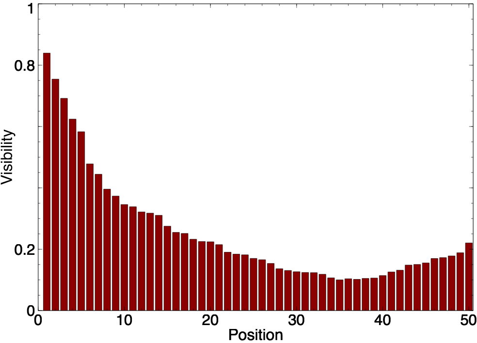
Figure 1: The visibility $v_{p}$ (y-axis) of position $p$ in the song list (x-axis) where $p=1$ is the top position and $p=50$ is the bottom position of the list which is displayed in a single column.

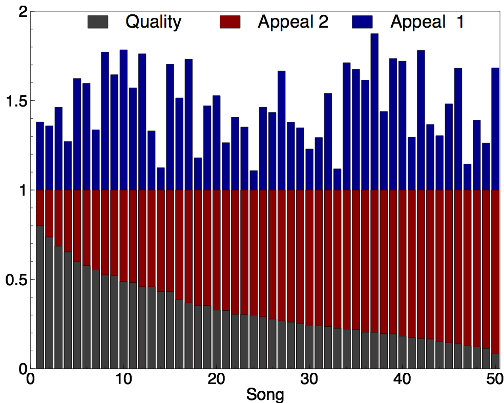
Figure 2: The quality $q_{i}$ (grey) and appeal $a_{i}$ (red and blue) of song $i$ in the two settings. The settings only differ in the appeal of songs, and not in the quality of songs. In the first setting, the quality and the appeal for the songs were chosen independently according to a Gaussian distribution normalised to fit between 0 and 1. The second setting explores an extreme case where the appeal is anti-correlated with the quality used in setting 1. In this second setting, the appeal and quality of each song sum to 1.

The agent-based simulation aims at emulating the MusicLab: Each simulation consists of $L$ iterations ($L$ simulated users ) and, at each iteration $t:0<t<L$,

1. the simulator randomly selects a song $i$ according to the probabilities $P_{i}(\sigma,\phi)$, where $\sigma$ is the ranking proposed by the policy under evaluation and $\phi$ represents the market shares;

2. the simulator randomly determines, with probability $q_{i}$, whether selected song $i$ is downloaded. In the case of a download, the simulator increases the number of downloads of song $i$, i.e., $d_{i}^{t+1}=d_{i}^{t}+1$, changing the market shares. Otherwise, $d_{i}^{t+1}=d_{i}^{t}$.

Every $t>0$ iterations, a new list $\sigma$ may be recomputed if the ranking policy is dynamic (e.g., the popularity ranking). In this paper, the simulation setting focuses mostly on two policies for ranking the songs:

• The quality ranking (Q-rank) that assigns the songs in decreasing order of quality to the positions in decreasing order of visibility (i.e., the highest quality song is assigned to the position with the highest visibility and so on);

• The popularity ranking (D-rank) that assigns the songs in decreasing order of popularity (i.e., $d_{i}^{t}$) to the positions in decreasing order of visibility (i.e., the most popular song is assigned to the position with the highest visibility and so on);

Note that the popularity ranking was used in the original MusicLab, while the quality ranking is a static policy: the ranking remains the same for the entire simulation. The simulation setting, which aims at being close to the MusicLab experiments, considers 50 songs and simulations with L=$10^{5}$ iterations unless stated otherwise. The songs are displayed in a single column. The analysis in [17] indicated that participants are more likely to try songs higher in the list. More precisely, the visibility decreases with the list position, except for a slight increase at the bottom positions. Figure 1 depicts the visibility profile based on these guidelines, which is used in all computational experiments. The paper also uses two settings for the quality and appeal of each song, which are depicted in Figure 2. In the first setting, the quality and the appeal were chosen independently according to a Gaussian distribution normalised to fit between $0$ and $1$. The second setting explores an extreme case where the appeal is anti-correlated with quality: The quality is the same as in the first setting but the appeal is chosen such that the sum of appeal and quality is 1.

6.1 Convergence

We first illustrate the convergence of the market for various popularity signals ($r<1$) using the quality ranking. In order to visualise the results, we focus on only 5 songs, where the qualities, appeals, and visibilities are given by

q = [ 0.80, 0.72, 0.68, 0.65, 0.60 ]

a = [ 0.38, 0.35, 0.46, 0.27, 0.62 ]

v = [ 0.80, 0.75, 0.69, 0.62, 0.58 ].

The simulation is run for $10^{5}$ iterations for the social signals $f(x)=x^{r}(r\in\{0.1,0.25,0.5,0.75\})$ and Figure 3 depicts the simulation results. Observe that the equilibrium $\phi^{*}$ (dashed lines) changes because it depends of the value of $r$. Interestingly, for social signals with $r\leq 0.5$, the convergence of the process seems to occur around $10^{4}$ time steps (iterations) even when they start with a strong initial distortion due to the appeals of the songs. The simulations show clear differences in behaviour depending on $r$ and, when $r$ moves closer to 1, the market tends to exhibit a monopolistic behaviour for the song with the best quality (confirming the results obtained in [32]).

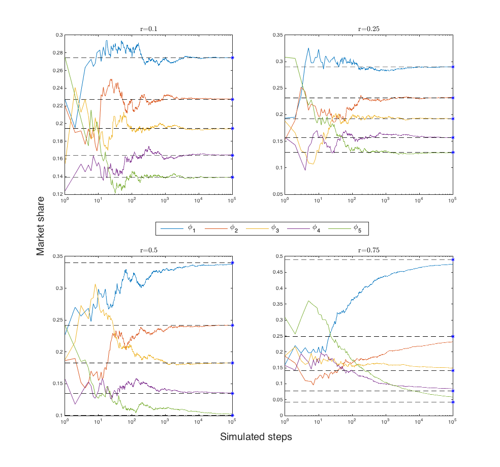
Figure 3: Evolution of market shares of 5 songs using a social signal $f(x)=x^{r},\quad r\in\{0.1,0.25,0.5,0.75\}$. Dashed lines are the values of the equilibrium for each song.

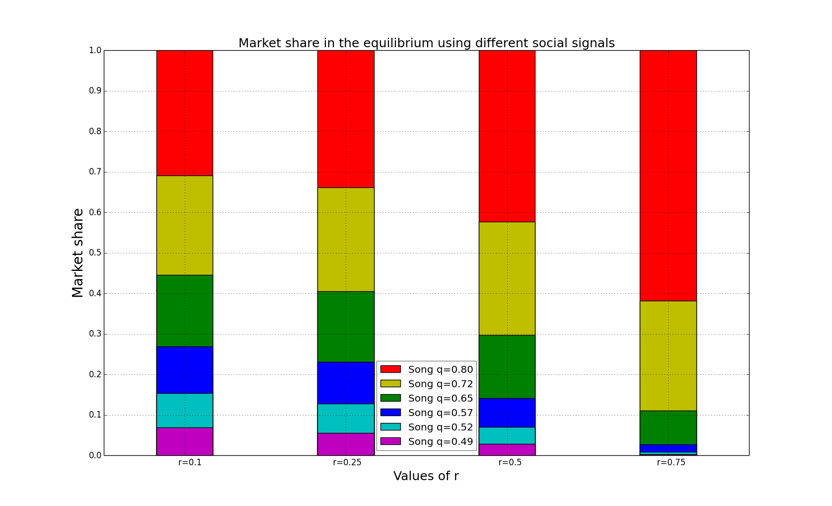
Figure 4: Market shares of 6 songs and their qualities, using a social signal $f(x)=x^{r},\quad r\in\{0.1,0.25,0.5,0.75\}$.

Figure 4 shows how the market is distributed in the equilibrium among 6 songs. The qualities, appeals, and visibilities are given by

q = [0.80, 0.72, 0.65, 0.57, 0.52, 0.49]

a = [0.38, 0.36, 0.27, 0.60, 0.77, 0.78]

v = [0.80, 0.75, 0.62, 0.48, 0.40, 0.35]

and the social signals are of the form $f(x)=x^{r}$ $(r\in\{0.1,0.25,0.5,0.75\})$. Each stacked bar represents the proportion of the market for the 6 songs for a given social signal. Songs with better qualities (i.e., the top 2 songs represented in red and yellow respectively) have larger market shares and their market shares increase with $r$. In contrast, the market shares of the lower-quality songs (i.e., cyan and purple respectively) decrease when $r$ increases. These results indicate that social influence has a beneficial effect on the market: it drives customers towards the better products, while not going to a monopoly as long as $r<1$.

6.2 Market Predictability

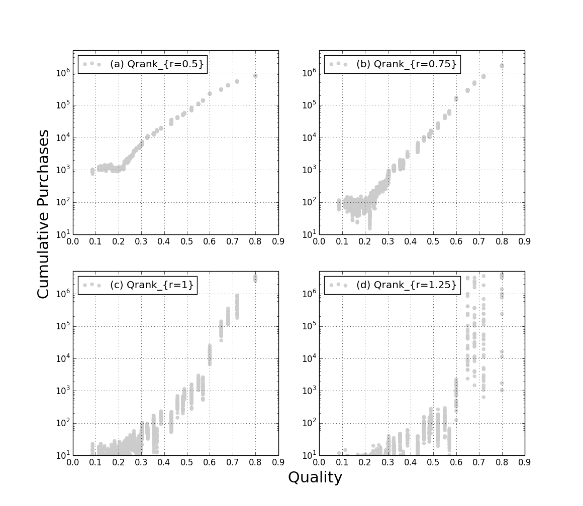
Figure 5: Distribution of downloads versus the qualities, using social signals $f(x)=x^{r},\quad r\in\{0.5,0.75,1,1.25\}$. The results are for the first setting where the quality and appeal of each song are chosen independently. The songs are ordered by increasing quality along the x-axis. The y-axis is the number of downloads.

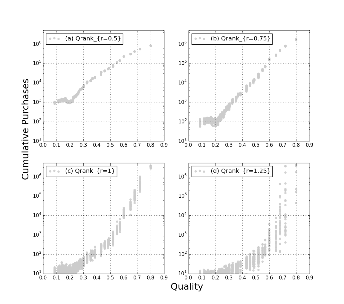
Figure 6: Distribution of downloads versus the qualities, using social signals $f(x)=x^{r},\quad r\in\{0.5,0.75,1,1.25\}$. The results are for the first setting where the quality and appeal of each song are anti-correlated. The songs are ordered by increasing quality along the x-axis. The y-axis is the number of downloads.

This section depicts the predictability of the market for various values of $r$ and the number of downloads per song as a function of its quality. Figures 5 and 6 depict the results for the two quality/appeal settings discussed previously. The figures display the results of 40 experiments for each setting with 1 million arrivals. Each experiment contributes 50 data points, i.e., the number of downloads for each song, and all the data points for the 40 experiments are displayed in the figures.

In the plots, the x-axis represents the song qualities and the y-axis the number of downloads. A dot at location $(q,d)$ indicates that the song with quality $q$ had $d$ downloads in an experiment. Obviously, there can be several dots at the same location. For $r\in\{0.5,0.75,1\}$, the market is highly predictable and there is little variation in the song downloads. For $r=1$, the market converges to a monopoly for the song of highest quality, confirming the results from [1, 32]. Finally, for $r=1.25$, the market exhibits significant unpredictability, as suggested by the theoretical results. In this case, the equilibria are monopolies for various songs but it is hard to predict which song will dominate the market.

Note also that the unpredictability of the market increases significantly for $r=1.25$ when the appeal and quality of the songs are anti-correlated. This is not the case for $r\in\{0.5,0.75\}$. To evaluate the statistical significance of these results, we measure the market unpredictability as suggested by Salganik et al. [26]. The unpredictability $u_{i}$ for product $i$ is defined as the average difference in market share for that product over the 40 experiments:

$$u_{i}=\frac{1}{\left(\begin{array}[]{c}40\\ 2\end{array}\right)}\sum_{w=1}^{40}\sum_{w^{*}=w+1}^{40}|\phi_{i,w}-\phi_{i,w^{*}}|,$$

where $\phi_{i,w}$ is the final market share of product $i$ in experiment $w$. We then computed the overall unpredictability for each social signal $r\in\{0.5,0.75,1,1.25\}$: $U=\dfrac{\sum_{j=1}^{n}u_{j}}{n}.$

Figure 7 shows the average unpredictability $U$ and the standard deviation for the different social signals, using the same data as in Figures 5 and 6 (Figure 7 $\mathsf{a}$ and Figure 7 $\mathsf{b}$ respectively). We also performed Mann-Whitney U tests, comparing the values of $U$ for pairs of social signals. In all cases, a social signal $r<1$ is significantly more predictable than the signal $r=1.25$ ($p$-value<0.05). Comparisons between $r=0.5$ and $r=0.75$ and $r=0.75$ and $r=1$ also show statistically significant differences in unpredictability. For instance, for the anti-correlated setting, the $p$-values for the various pairwise comparisons (first column is less unpredictable than second column) are given in Table 1

social signal	social signal	$p$-value
0.5	0.75	0.0029
0.5	1	8.73e-07
0.5	1.25	4.24e-10
0.75	1	0.0003
0.75	1.25	2.10e-07
1	1.25	0.0022

Table 1: p-values of the hypothesis: first column is less predictable than second column. Case $a_{i},q_{i}$ anti-correlated.

For the independent setting, Table 2 shows the pairwise comparisons that are also statistically significant in that case:

social signal	social signal	p-value
0.5	1	0.0414
0.5	1.25	0.0034
0.75	1.25	0.0266

Table 2: p-values of the hypothesis: first column is less predictable than second column. Case $a_{i},q_{i}$ independent.

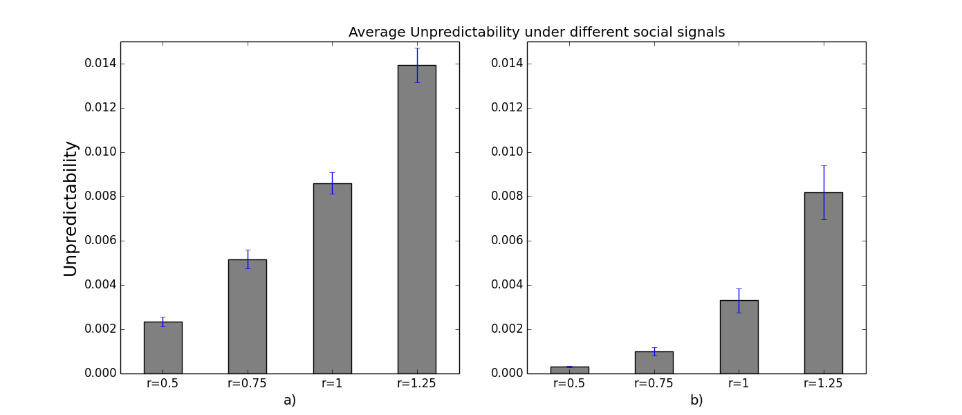
Figure 7: Average unpredictability (grey bars), using social signals $f(x)=x^{r},\quad r\in\{0.5,0.75,1,25\}$. $\mathsf{a})$ shows the results for the independent setting, and $\mathsf{b})$ for the anti-correlated setting. Both cases consist of 40 experiments with 1 million iterations each. Blue lines represent the respective standard deviations.

Figure 8 compares the predictability of Q-rank and D-rank for the first setting of Quality/Appeal. For each ranking, two different social signals were used ($r=0.5$ and $r=1$) and the figure displays the result of 50 experiments, consisting in 1 million iterations. Two phenomena can be observed. First, sublinear signals seem to help the D-rank, making the outcome less chaotic (first column). Second, Q-rank clearly performs better than D-rank and exhibits much less unpredictability.

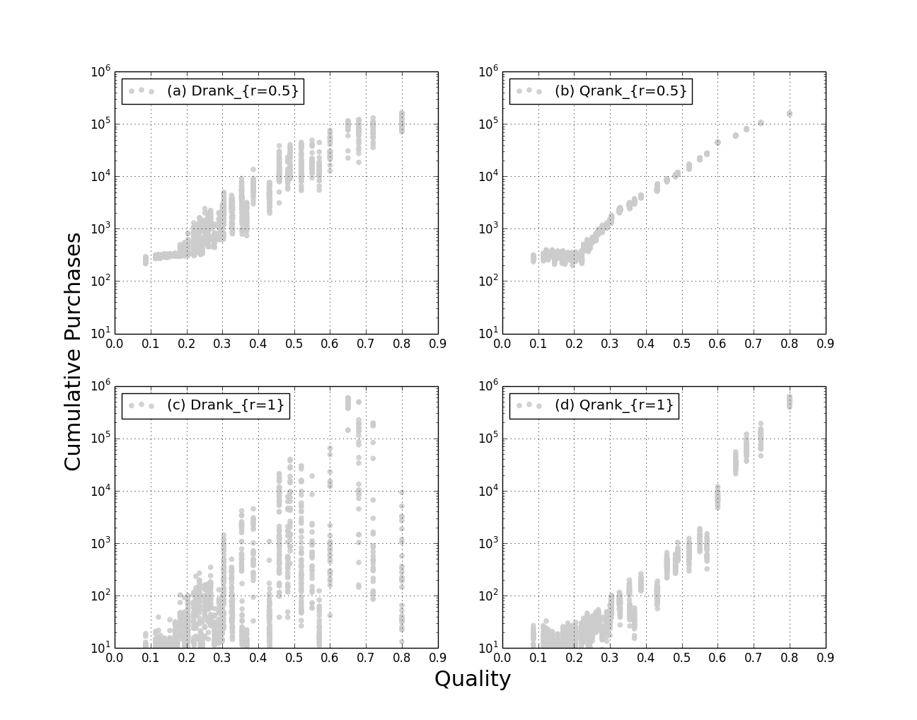
Figure 8: Distribution of purchases versus product qualities for 50 experiments with 1 million users. Figures (a) and (b) use a social signal $f(x)=x^{0.5}$, Figure (a) shows the results for the popularity ranking and Figure (b) for the quality ranking. Figures (c) and (d) use the social signal $f(x)=x$, Figure (c) shows the results for the popularity ranking and Figure (d) for the quality ranking.

6.3 Performance of the Market

Figures 9 and 10 report results about the performance of the markets as a function of the social influence signals. The figures report the average number of downloads over time among 50 experiments, for the quality and popularity rankings as a function of the social signals. There are a few observations that deserve mention.

1. For the quality ranking, the expected number of downloads increases with the strength of the social signal as $r$ approaches 1. The equilibrium when $r=1$ is optimal asymptotically and assigns the entire market share to the song of highest quality. When $r=2$, the situation is more complicated. The figure shows that the market efficiency can further improve if $r=2$. However, when the simulation is run for more iterations (a result not shown in the figure), the market efficiency decreases slightly compared to $r=1$, which is consistent with the theory since there is no guarantee that the monopoly for $r>1$ is for the song of highest quality.

2. The popularity ranking is always dominated by the quality ranking and the benefits of the quality ranking increase as $r$ approaches 1 from below.

3. The popularity ranking in the second setting when $r=2$, obtains nearly a third of the expected downloads than the quality ranking.

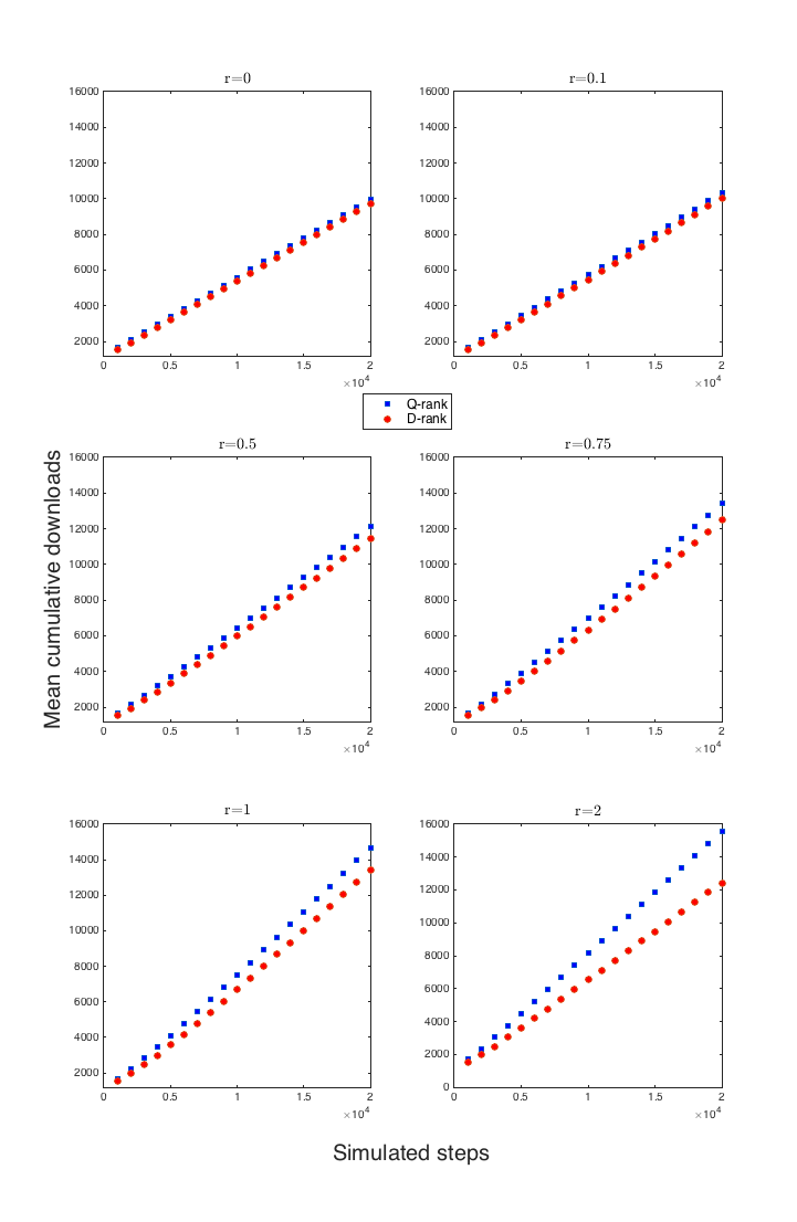
Figure 9: The Average Number of Downloads over Time for the Quality and Popularity Rankings for Various Social Signals in the First Setting for Song Appeal and Quality.

Figure 10: The Average Number of Downloads over Time for the Quality and Popularity Rankings for Various Social Signals in the Second Setting for Song Appeal and Quality.

7 Additional Observations on Sublinear Social Signals

The Benefits of Social Influence

A linear social signal has been shown to be beneficial to the market efficiency, i.e. it maximises the expected number of downloads. This result was proved by [1] for the performance ranking and by [32] for any static ranking such as the quality ranking. Unfortunately, sublinear social signals are not always beneficial to the market in that sense, as one can see in Example 7.1. Consider, once again, the quality ranking and assume that $q_{1}\geq\ldots\geq q_{n}$. When there is no social signal, by following the idea in Equation (3) and taking $f(\phi_{i})=\beta\phi_{i}+\alpha a_{i}$, with $\beta=0$, the probability of trying product $i$ is given by

$$p_{i}^{I}=\frac{v_{i}a_{i}}{\sum_{j=1}^{n}v_{j}a_{j}}.$$

In this case, the expected number of purchases per period is

$$\sum_{i=1}^{n}p_{i}^{I}q_{i}.$$

On the other hand, with a social signal, the probability of trying product $i$ at time $t$ is

$$P_{i}(\phi^{t})=\frac{v_{i}f(\phi_{i}^{t})}{\sum_{j=1}^{n}v_{j}f(\phi_{j}^{t})}$$

and the expected number of purchases per period at the equilibrium is given by

$$\sum_{i=1}^{n}P_{i}(\phi^{*})q_{i}=\sum_{i=1}^{n}\frac{v_{i}q_{i}f(\phi_{i}^{*})}{\sum_{j=1}^{n}v_{j}f(\phi_{j}^{*})}.$$

The following example shows that, under a sublinear social signal, the expected number of purchases (per period) at equilibrium, i.e., $\sum_{i=1}^{n}P_{i}(\phi^{*})q_{i}$, can be lower than the expected number of purchases when no social signal is used, i.e., $\sum_{i=1}^{n}p_{i}^{I}q_{i}.$

Example 7.1.

Consider a 2-dimensional T-O market with social signal $f(x)=x^{0.5}$, where the qualities, visibilities, and appeals are given by

• $q_{1}=1$, $q_{2}=0.4$,

• $v_{1}=1$, $v_{2}=1$,

• $a_{1}=1$, $a_{2}=0.3$.

The expected number of purchases at equilibrium for the case with social signal is given by

$$\frac{v_{1}q_{1}(\phi_{1}^{*})^{r}+v_{2}q_{2}(\phi_{2}^{*})^{r}}{v_{1}(\phi_{1}^{*})^{r}+v_{2}(\phi_{2}^{*})^{r}}=\frac{v_{1}q_{1}(v_{1}q_{1})^{r/(1-r)}+v_{2}q_{2}(v_{2}q_{2})^{r/(1-r)}}{v_{1}(v_{1}q_{1})^{r/(1-r)}+v_{2}(v_{2}q_{2})^{r/(1-r)}}=\frac{1+(0.4)^{2}}{1+0.4}\sim 0.83,$$

while, for the case without social signal, it is given by

$$\frac{v_{1}q_{1}a_{1}+v_{2}q_{2}a_{2}}{v_{1}a_{1}+v_{2}a_{2}}=\frac{1+0.3(0.4)}{1+0.3}\sim 0.86.$$

This simple example, in which the qualities and appeals are positively correlated, shows that if customers follow a sublinear social influence signal ($r=0.5$), the market efficiency gets reduced by around 3 percent (with respect to not showing them the social signal). In contrast, when $r=1$, social influence drives the market towards a monopoly, which leads to an asymptotically optimal market that assigns the entire market share to the highest quality product (which may be undesirable in practice). Note that, once the qualities and appeals have been recovered (using, say, Bernoulli sampling as suggested in [1]), one could potentially decide whether to use the social influence (in case it is sublinear $r<1$): Simply compare the expected number of purchases in both settings, using the equilibrium for the social influence case and the formula for the case with no social signal.

Optimality of the Quality Ranking

When $r=1$, it has been shown that the quality ranking is optimal asymptotically: It maximises the expected number of purchases [32]. If another static ordering is used, the market will converge to the product that has the highest quality when scaled by its visibility. However, when $0<r<1$, the quality ranking is no longer guaranteed to be optimal asymptotically.

Example 7.2.

Consider a 3-dimensional T-O market with a social signal $f(x)=x^{r},r=0.3$, and the following values for qualities and visibilities:

• $q_{1}=1$, $q_{2}=0.261$, $q_{3}=0.002$

• $v_{1}=1$, $v_{2}=0.720$, $v_{3}=0.229$

then, using quality ranking we would end up with an expected number of purchases at equilibrium, given by

$$\sum_{i=1}^{n}P_{i}(\phi^{*})q_{i} =\frac{v_{1}q_{1}(v_{1}q_{1})^{r/(1-r)}+v_{2}q_{2}(v_{2}q_{2})^{r/(1-r)}+v_{3}q_{3}(v_{3}q_{3})^{r/(1-r)}}{v_{1}(v_{i}q_{i})^{r/(1-r)}+v_{2}(v_{2}q_{2})^{r/(1-r)}+v_{3}(v_{3}q_{3})^{r/(1-r)}}$$

$$=\frac{1+(0.720*0.261)^{10/7}+(0.229*0.002)^{10/7}}{1+0.720(0.720*0.261)^{3/7}+0.229(0.229*0.002)^{3/7}}\sim 0.8026,$$

on the other hand, if we decide to place the third product (quality $q_{3}=0.002$) in the second position, and the second product (quality $q_{2}=0.261$) in the third position of the ranking, we get

$$\sum_{i=1}^{n}P_{\sigma_{i}}(\phi^{*})q_{i} =\frac{v_{1}q_{1}(v_{1}q_{1})^{r/(1-r)}+v_{2}q_{3}(v_{2}q_{3})^{r/(1-r)}+v_{3}q_{2}(v_{3}q_{2})^{r/(1-r)}}{v_{1}(v_{i}q_{i})^{r/(1-r)}+v_{2}(v_{2}q_{3})^{r/(1-r)}+v_{3}(v_{3}q_{2})^{r/(1-r)}}$$

$$=\frac{1+(0.720*0.002)^{10/7}+(0.229*0.261)^{10/7}}{1+0.720(0.720*0.002)^{3/7}+0.229(0.229*0.261)^{3/7}}\sim 0.9154.$$

The intuition behind the previous example is that if there exists a product which is much better than the rest, the best decision is to exhibit it in the first position and place, in the second position, the lowest quality product to make the first product is even more appealing. It is an open problem to determine whether there is a polynomial-time algorithm to find an optimal ranking.

8 Discussion and Conclusion

This paper studied the role of social influence in trial-offer markets where customer preferences are modeled by a generalisation of a multinomial logit. In this model, both position bias and social influence impact the products tried by consumers.

The main result of the paper is to show that trial-offer markets, when the ranking of the products is fixed, converge to a unique equilibrium for sublinear social signals of the form $\phi_{i}^{r}$, where $\phi_{i}$ represents the cumulative market share of product $i$. Of particular interest is the fact that the equilibrium does not depend on the initial conditions, e.g., the product appeals, but only depends on the product qualities. Moreover, when the products are ranked by quality, i.e., the best products are assigned the highest visibilities, the equilibrium is such that the better products receive the largest market shares, which increase as $r$ increases for the best products (as long as $r<1$). The equilibrium for a sublinear social signal contrasts with the case with $r=1$, where the market goes to a monopoly for the highest quality product (under the quality ranking). In the sublinear case, the market shares reflect product quality but no product becomes a monopoly. The paper also shows that, when $r>1$, the market becomes more unpredictable. In particular, the inner equilibrium, which assigns a positive market share to all products, is unstable and the market is likely to converge to a monopoly for some product. However, which product becomes the monopoly depends on the initial conditions.

Simulation results on a setting close to the original MusicLab complemented the theoretical results. They show that the market converges quickly to the equilibrium for a sublinear social signal and that the convergence speed depends on the social signal strength. The simulation results also illustrate how the market shares of the highest (resp. lowest) quality products increase (resp. decrease) with $r$. As expected, when $r\leq 1$, the market is shown to be highly predictable, while it exhibits a lot of randomness when $r>1$. The simulation results also show the benefits of social influence for market efficiency, and demonstrate that the quality ranking once again outperforms the popularity ranking.

Overall, these results shed a new light on the role of social influence in trial-offer markets and provide a comprehensive overview of the choices and tradeoffs available to firms interested in optimising their markets with social influence. In particular, they show that social influence does not necessarily make markets unpredictable and is typically beneficial when the social signal is not too strong. Moreover, ranking the products by quality appears to be a much more effective policy than ranking products by popularity which may induce unpredictability and market inefficiency. The results also show that sublinear social signals give decision makers the ability to trade market efficiency for more balanced market shares.

Perhaps, the main contribution of this paper is to show that markets under social influence are very sensitive to various design choices. The findings in [26] used the popularity ranking, which significantly affected their conclusions about market unpredictability and efficiency. The theoretical and simulation results of this paper, together with those in [1, 32] for the case $r=1$, show that the market is highly predictable when using any static ranking and $r\leq 1$. Moreover, the quality ranking is optimal asymptotically when $r=1$ and dominates the popularity ranking in all our simulations which were modeled after the MusicLab. This does not diminish the value of the results by Salganik et al. [26] who isolated potential pathologies linked to social influence. But this paper shows that these pathologies are not inherent to the market but are a consequence of specific design choices in the experiment: The strength of the social signal and the ranking policy. Interestingly, it is only for a linear social signal that social influence can be shown to be always beneficial in expectation. Fortunately, for sublinear social signals, we can determine a priori if social influence is beneficial, given the analytic form of the equilibrium.

There are at least two potential research directions following this paper that worth investigating. First, it would be extremely valuable to construct large-scale cultural market experiment, varying the strengths of the social signal to complement our simulation results. Second, it would be interesting to extend our results to other settings including assortment problems (where the firm can select not only how to rank products but also which ones should be shown) [2] and to classical cascade models with a social signal [34].

Appendix A Key Results from Benaïm (1999) [6]

Consider the set of solutions of the differential equation (9), we say that $\Upsilon=(\Upsilon_{t})_{t\in\mathbb{R}}$ is the flow induced by the vector field $F$, where $\Upsilon_{t}$ are the local unique solutions of (9) with $x^{0}=x_{0}\in\Delta^{n-1}$. Benaïm defines the following useful concept: A continuous function $X:\mathbb{R}_{+}\to\mathbb{R}^{n}$ is an Asymptotic pseudo-trajectory for $\Upsilon$ if for any $T>0$

$$\lim_{t\to\infty}\sup_{0\leq h\leq T}dist(X(t+h),\Upsilon_{h}(X(t)))=0.$$

Recall now that our Robbins-Monro Algorithm (8) is defined by

$$\phi^{k+1}=\phi^{k}+\gamma^{k+1}(F(\phi^{k})+U^{k+1}).$$

Let $\tau_{k}=\sum_{i=1}^{k}\gamma^{i},\tau_{0}=0$ and define the affine interpolated process $Z(t)$:

$$Z(t)=\phi^{k}+[t-\tau_{k}]\frac{\phi^{k+1}-\phi^{k}}{\gamma^{k+1}},\quad\tau_{k}\geq t\geq\tau_{k+1}.$$ (20)

Consider also the map $m:\mathbb{R}_{+}\to\mathbb{N}$ defined by $m(t)=\sup\{k\geq 0:t\geq\tau_{k}\}$.

Proposition A.1 (Proposition 4.1 in [6]).

Let $F$ be a bounded locally Lipschitz vector field. Assume that

1. For all $T>0$,

   $$\lim_{l\to\infty}\sup\{\|\sum_{i=n}^{k-1}\gamma^{i+1}U^{i+1}\|:k=n+1,...,m(\tau_{l}+T)\}=0.$$

2. $\displaystyle\sup_{k}\|\phi^{k}\|<\infty.$

Then the interpolated process $Z(t)$ is an asymptotic pseudotrajectory of the flow induced by $F$.

Proposition A.2 (Proposition 4.2 in [6]).

Let $\phi^{k}$ be the Robbins-Monro Algorithm (8). Suppose that, for some $q\geq 2$,

$$\sup_{k}\mathbb{E}(\|U^{k+1}\|^{q})<\infty,$$

and

$$\sum_{k}[\gamma^{k}]^{1+q/2}<\infty.$$

Then assumption $A1.1$ of Proposition A.1 holds with probability 1.

Let $X:\mathbb{R}_{+}\to M$ be an asymptotic pseudotrajectory of an induced flow $\Phi$, with $M$ some metric space. The limit set $L(X)$ of $X$ is the set of limits of convergent sequences $X(t_{k})$, $t_{k}\to\infty$.

Theorem A.3 (Theorem 5.7 $i)$ in [6]).

Let $X$ be a precompact asymptotic pseudotrajectory of $\Phi$. Then $L(X)$ is Internally Chain Transitive.

Appendix B Proofs

Proof of Lemma 3.1.

The probability that item $i$ is purchased in the first step is given by

$$p_{i}^{1st}(\phi)=\frac{v_{i}f(\phi_{i})}{\sum\limits_{j=1}^{n}v_{j}f(\phi_{j})}q_{i}.$$

The probability that item $i$ is purchased in the second step and no item was purchased in the first step is given by

$$p_{i}^{2nd}(\phi)=\left(\frac{\sum\limits_{j=1}^{n}v_{j}f(\phi_{j})(1-q_{j})}{\sum\limits_{j=1}^{n}v_{j}f(\phi_{j})}\right)\frac{v_{i}f(\phi_{i})}{\sum\limits_{j=1}^{n}v_{j}f(\phi_{j})}q_{i}.$$

More generally, the probability that item $i$ is purchased in step $m$ while no item was purchased in earlier steps is given by

$$p_{i}^{mth}(\phi)=\left(\frac{\sum\limits_{j=1}^{n}v_{j}f(\phi_{j})(1-q_{j})}{\sum\limits_{j=1}^{n}v_{j}f(\phi_{j})}\right)^{m-1}\frac{v_{i}f(\phi_{i})}{\sum\limits_{j=1}^{n}v_{j}f(\phi_{j})}q_{i}.$$ (21)

Let $a=(\sum\limits_{j=1}^{n}v_{j}f(\phi_{j})q_{j})/(\sum\limits_{j=1}^{n}v_{j}f(\phi_{j}))$. Observe that, if $q_{max}=\max_{i\in\{1,...,n\}}q_{i}$, then $0<a\leq q_{max}\leq 1$. Equation (21) becomes

$$p_{i}^{mth}(\phi)=\bigg{(}1-a\bigg{)}^{m-1}\frac{v_{i}f(\phi_{i})}{\sum\limits_{j=1}^{n}v_{j}f(\phi_{j})}q_{i}.$$

Hence the probability that the next purchase is item $i$ is given by

$$p_{i}(\phi)=\sum\limits_{m=0}^{\infty}\bigg{(}1-a\bigg{)}^{m}\frac{v_{i}f(\phi_{i})}{\sum\limits_{j=1}^{n}v_{j}f(\phi_{j})}q_{i}.$$

Since $|1-a|<1$, we use the geometric series

$$\sum\limits_{m=0}^{\infty}\bigg{(}1-a\bigg{)}^{m}=\frac{1}{a},$$

and then, the probability that the next purchase is item $i$ is given by

$$p_{i}(\phi)=\frac{v_{i}q_{i}f(\phi_{i})}{\sum\limits_{j=1}^{n}v_{j}q_{j}f(\phi_{j})}.$$

∎

Proof Theorem 4.10.

Thanks to $H1-H2$, Proposition A.2 holds for $q=2$. As a result, we can apply Proposition A.1 and $Z(t)$ from Equation (20) is almost surely an asymptotic pseudo-trajectory for the flow induced by $F$. As $x^{t}\in\Delta^{n-1}$, then $Z(t)$ is precompact. Finally, using Theorem A.3, the limit set $L\{x^{t}\}_{t\geq 0}$ is an ICT for Equation (9). ∎

Appendix C Market Shares Versus Purchases

The condition $d_{i}^{0}=a_{i}$ can be relaxed and the results still hold but the notations become more complicated. Indeed, define the variables $\mu_{i}^{k}=\frac{a_{i}+d_{i}^{k}}{\sum_{j}a_{j}+d_{j}^{k}}$, with $d_{i}^{0}=0$, consider $\hat{a}=\sum_{j=1}^{n}a_{i}$ the cumulative appeal, and $\mathbf{a},\mathbf{d^{k}}$ the vectors of appeals and purchases respectively. By definition $\sum_{j=1}^{n}d_{j}^{k}=k$, then we can define the probability function $p(\mu^{k})$ by

$$p_{i}(\mu^{k})=\frac{v_{i}q_{i}f(\mu_{i}^{k})}{\sum_{j=1}^{n}v_{j}q_{j}f(\mu_{j}^{k})},\quad i\in\{1,...,n\}$$

and recover a recurrence for $\mu$ as follows:

$$\mu^{k+1} =\frac{\mathbf{a+d^{k}}}{\hat{a}+k+1}+\frac{e^{k}}{\hat{a}+k+1}$$

$$=\frac{\mathbf{a+d^{k}}}{\hat{a}+k}\frac{\hat{a}+k}{\hat{a}+k+1}+\frac{e^{k}}{\hat{a}+k+1}$$

$$=\mu^{k}\frac{\hat{a}+k}{\hat{a}+k+1}+\frac{e^{k}}{\hat{a}+k+1}$$

$$=\mu^{k}\frac{\hat{a}+k+1}{\hat{a}+k+1}-\frac{\mu^{k}}{\hat{a}+k+1}+\frac{e^{k}}{\hat{a}+k+1}$$

$$=\mu^{k}+\frac{1}{\hat{a}+k+1}(p(\mu^{k})-\mu^{k}+e^{k}-\mathbb{E}[e^{k}|\mathcal{F}^{k}])$$

$$=\mu^{k}+\hat{\gamma}^{k+1}[\hat{F}(\mu^{k})+\hat{U}^{k+1}].$$

In consequence, all the results from this paper can be translated from the $\phi$ domain to the $\mu$ domain.

Appendix D Dataset

Table 3 shows the values of the qualities and appeals for the independent setting (obtained from [1]). Table 4 shows the values of the visibilities for each position $j\in\{1,\dots,n\}$.

Product	Quality	Appeal	Product	Quality	Appeal
1	0.8	0.18581654	26	0.278009	0.35136515
2	0.72	0.28594501	27	0.2673	0.78687609
3	0.68	0.52073051	28	0.26083	0.7369193
4	0.65	0.81398644	29	0.2512	0.75227893
5	0.60	0.45868017	30	0.24396	0.32580804
6	0.57	0.15955483	31	0.23941	0.30674759
7	0.55	0.43715743	32	0.23622	0.91103217
8	0.52005	0.38484972	33	0.22629	0.76236248
9	0.52	0.63739211	34	0.2214	0.11459921
10	0.4887	0.78174105	35	0.22013	0.7581713
11	0.48224	0.52983037	36	0.20418	0.76994571
12	0.4586	0.6382574	37	0.20389	0.67408264
13	0.45837	0.80597	38	0.19535	0.41759683
14	0.432	0.2520265	39	0.1947	0.68898008
15	0.43067	0.37266718	40	0.18248	0.82117398
16	0.38623	0.79358615	41	0.17444	0.33890645
17	0.36792	0.19972853	42	0.16867	0.63497574
18	0.35492	0.32368825	43	0.16638	0.16224351
19	0.35374	0.94736709	44	0.15374	0.47778872
20	0.32799	0.50704873	45	0.14542	0.23702317
21	0.32589	0.7105828	46	0.1387	0.49406539
22	0.30411	0.92616787	47	0.12764	0.45956048
23	0.30352	0.64768258	48	0.12217	0.75210134
24	0.29988	0.51815068	49	0.11418	0.66488509
25	0.2905	0.47170285	50	0.08636	0.80257928

Table 3: Values of quality and appeal for the products in the independent case. Recall that the values of the appeal in the anti-correlated setting are given by $a_{i}=1-q_{i}$.

Position	Visibility	Position	Visibility
1	0.83	25	0.16583292
2	0.75	26	0.15370582
3	0.69	27	0.13640378
4	0.62	28	0.13084858
5	0.58	29	0.12666812
6	0.48	30	0.12429217
7	0.44	31	0.12362827
8	0.4	32	0.11847651
9	0.37	33	0.10675012
10	0.35	34	0.1001895
11	0.338	35	0.10377821
12	0.321	36	0.10192779
13	0.317	37	0.10484361
14	0.31063943	38	0.10609265
15	0.2750814	39	0.11420125
16	0.25493054	40	0.1260095
17	0.25148059	41	0.13163135
18	0.23254506	42	0.14843575
19	0.22517471	43	0.15040223
20	0.22429915	44	0.15529018
21	0.21502087	45	0.1699023,
22	0.19038769	46	0.17265442
23	0.18407585	47	0.17825863
24	0.18185429	48	0.18851792
25	0.17013229	50	0.22057129

Table 4: Values of the visibilities for each position $j\in\{1,\dots,n\}$.

References

- [1] A. Abeliuk, G. Berbeglia, M. Cebrian, and P. Van Hentenryck. The benefits of social influence in optimized cultural markets. PLoS ONE, 10(4), 2015.
- [2] A. Abeliuk, G. Berbeglia, M. Cebrian, and P. Van Hentenryck. Assortment optimization under a multinomial logit model with position bias and social influence. 4OR, 14(1):57–75, 2016.
- [3] A. Abeliuk, G. Berbeglia, F. Maldonado, and P. Van Hentenryck. Asymptotic optimality of myopic optimization in trial-offer markets with social influence. In In the 25th International Joint Conference on Artificial Intelligence (IJCAI-16), New York, NY, July 9-15, 2016.
- [4] A. Abeliuk, G. Berbeglia, P. Van Hentenryck, T. Hogg, and K. Lerman. Taming the unpredictability of cultural markets with social influence. In Proceedings of the 26th International Conference on World Wide Web, pages 745–754. International World Wide Web Conferences Steering Committee, 2017.
- [5] E. Altszyler, F. Berbeglia, G. Berbeglia, and P. Van Hentenryck. Transient dynamics in trial-offer markets with social influence: Trade-offs between appeal and quality. PloS one, 12(7):e0180040, 2017.
- [6] M. Benaïm. Dynamics of stochastic approximation algorithms. In Seminaire de probabilites XXXIII, pages 1–68. Springer, 1999.
- [7] V. S. Borkar and S. P. Meyn. The ODE method for convergence of stochastic approximation and reinforcement learning. SIAM Journal on Control and Optimization, 38(2):447–469, 2000.
- [8] S. Ceyhan, M. Mousavi, and A. Saberi. Social influence and evolution of market share. Internet Mathematics, 7(2), 2011.
- [9] F. Chung, S. Handjani, and D. Jungreis. Generalizations of Pólya’s urn problem. Annals of Combinatorics, 7:141–153, 2003.
- [10] C. Conley. Isolated invariant sets and the morse index. In CBMS Regional Conference Series in Mathematics, 38, volume 16, 1978.
- [11] N. Craswell, O. Zoeter, M. Taylor, and B. Ramsey. An experimental comparison of click position-bias models. In Proceedings of the 2008 International Conference on Web Search and Data Mining, pages 87–94. ACM, 2008.
- [12] M. Duflo and S. S. Wilson. Random iterative models, volume 22. Springer Berlin, 1997.
- [13] P. Engstrom and E. Forsell. Demand effects of consumers’ stated and revealed preferences. Available at SSRN 2253859, 2014.
- [14] M. W. Hirsch, S. Smale, and R. L. Devaney. Differential equations, dynamical systems, and an introduction to chaos. Academic press, 2012.
- [15] M. Hu, J. Milner, and J. Wu. Liking and following and the newsvendor: Operations and marketing policies under social influence. Management Science, 62(3):867–879, 2015.
- [16] D. W. Jordan and P. Smith. Nonlinear ordinary differential equations: an introduction to dynamical systems, volume 2. Oxford University Press, USA, 1999.
- [17] C. Krumme, M. Cebrian, G. Pickard, and S. Pentland. Quantifying social influence in an online cultural market. PLoS ONE, 7(5), 2012.
- [18] H. J. Kushner and G. Yin. Stochastic approximation and recursive algorithms and applications, volume 35. Springer Science; Business Media, 2003.
- [19] K. Lerman and T. Hogg. Leveraging position bias to improve peer recommendation. PLoS ONE, 9(6), 2014.
- [20] A. Lim, B. Rodrigues, and X. Zhang. Metaheuristics with local search techniques for retail shelf-space optimization. Management Science, 50(1):117–131, 2004.
- [21] L. Ljung. Analysis of recursive stochastic algorithms. IEEE Trans. Autom. Control,, 22(4):551–575, 1977.
- [22] H. Mahmound. Pólya Urn Models. Chapman & Hall/CRC Texts in Statistical Science, 2008.
- [23] L. Muchnik, S. Aral, and S. J. Taylor. Social influence bias: A randomized experiment. Science, 341(6146):647–651, 2013.
- [24] H. Renlund. Generalized Pólya Urns Via Stochastic Approximation. ArXiv e-prints 1002.3716, Feb. 2010.
- [25] D. J. Robinson. A course in linear algebra with applications. World Scientific, 2006.
- [26] M. J. Salganik, P. S. Dodds, and D. J. Watts. Experimental study of inequality and unpredictability in an artificial cultural market. Science, 311(5762):854–856, 2006.
- [27] M. J. Salganik and D. J. Watts. Leading the herd astray: An experimental study of self-fulfilling prophecies in an artificial cultural market. Social Psychology Quarterly, 71(4):338–355, 2008.
- [28] M. J. Salganik and D. J. Watts. Web-based experiments for the study of collective social dynamics in cultural markets. Topics in Cognitive Science, 1(3):439–468, 2009.
- [29] C. Stummer, E. Kiesling, M. Günther, and R. Vetschera. Innovation diffusion of repeat purchase products in a competitive market: an agent-based simulation approach. European Journal of Operational Research, 245(1):157–167, 2015.
- [30] C. Tucker and J. Zhang. How does popularity information affect choices? a field experiment. Management Science, 57(5):828–842, 2011.
- [31] A. van de Rijt, S. M. Kang, M. Restivo, and A. Patil. Field experiments of success-breeds-success dynamics. Proceedings of the National Academy of Sciences, 111(19):6934–6939, 2014.
- [32] P. Van Hentenryck, A. Abeliuk, F. Berbeglia, G. Berbeglia, and F. Maldonado. Aligning popularity and quality in online cultural markets. In In the Proceedings of the International AAAI Conference on Web and Social Media (ICWSM 2016), Cologne, Germany, May, 2016.
- [33] G. Viglia, R. Furlan, and A. Ladrón-de Guevara. Please, talk about it! when hotel popularity boosts preferences. International Journal of Hospitality Management, 42:155–164, 2014.
- [34] C. Wang, W. Chen, and Y. Wang. Scalable influence maximization for independent cascade model in large-scale social networks. Data Mining and Knowledge Discovery, 25(3):545–576, 2012.
- [35] X. Yuan and H. B. Hwarng. Stability and chaos in demand-based pricing under social interactions. European Journal of Operational Research, 253(2):472–488, 2016.