Efficient Thresholded Correlation using Truncated Singular Value Decomposition

Abstract

Efficiently computing a subset of a correlation matrix consisting of values above a specified threshold is important to many practical applications. Real-world problems in genomics, machine learning, finance other applications can produce correlation matrices too large to explicitly form and tractably compute. Often, only values corresponding to highly-correlated vectors are of interest, and those values typically make up a small fraction of the overall correlation matrix. We present a method based on the singular value decomposition (SVD) and its relationship to the data covariance structure that can efficiently compute thresholded subsets of very large correlation matrices.

1 Introduction

Finding highly-correlated pairs among a large set of vectors is an important part of many applications. For instance, subsets of highly-correlated vectors of gene expression values may be used in the discovery of networks of genes relevant to particular biological processes [13]. Identification of highly-correlated pairs may be used in feature selection algorithms for machine learning applications [5, 17] and are important to time series and image processing applications [11, 14].

The number of correlation coefficients grows quadratically with the number of vectors. Simply computing all pairs of correlation coefficients and then filtering out coefficients below a given threshold may not be computationally feasible for high-dimensional data in modern genomics and other applications. Considerable attention has been devoted to pruning methods that cheaply prune away all but the most highly-correlated pairs of vectors. For example the TAPER and related algorithms of Xiong et al. develop pruning rules based on the frequency of mutually co-occurring observations (rows) among vector pairs; see [16, 15] and the references therein. Related methods approximate a set containing the most highly-correlated pairs using hashing algorithms [18]. A number of other methods arrive at approximate sets of the most highly-correlated pairs using dimensionality-reduction techniques like the discrete Fourier transform [11]. The method of Wu, et al. [14], conceptually very similar to our approach, uses the singular value decomposition (SVD) to find all pairs of close vectors with respect to a distance metric (instead of correlation). Hero and Rajaratnam[6] apply projections to the thresholded correlation problem with the additional objective of determining a reasonable threshold value; their method follows a probabilistic approach. Our method finds all of the most highly-correlated vector pairs with respect to a given threshold by pruning along an intuitive path of decreasing variance defined by the data and computed by a truncated SVD.

Consider a real-valued data matrix $A$ consisting of $m$ observations of $n$ column vectors. Denote the columns of $A$ as $a_{j}\in\mathcal{R}^{m}$ for $j=1,2,\ldots,n$, $A=[a_{1},a_{2},\ldots,a_{n}]\in\mathcal{R}^{m\times n}$, and let $k=\mathrm{rank}(A)$. Assume that the mean of each column $a_{j}$ is zero and that each column has unit norm $\|a_{j}\|=1$. Here and below, $\|\cdot\|$ denotes the Euclidean vector norm. Then the Pearson sample correlation matrix $\mathrm{cor}(A)=A^{T}A$. Note that under these assumptions the sample correlation and covariance matrices are the same up to a constant multiple. Section 3 illustrates how to relax the unit norm and zero mean assumptions in practice.

Let $A=U\Sigma V^{T}$ be a singular value decomposition of $A$, where $U\in\mathcal{R}^{m\times k}$, $V\in\mathcal{R}^{n\times k}$, $U^{T}U=V^{T}V=I$, and $\Sigma\in\mathcal{R}^{k\times k}$ is a diagonal matrix with diagonal entries $\sigma_{1}\geq\sigma_{2}\geq\cdots\geq\sigma_{k}>0$. For later convenience, we write $s_{1:p}=[\sigma_{1},\sigma_{2},\ldots,\sigma_{p}]^{T}$ to be the vector of the first $p\leq k$ singular values along the diagonal of $\Sigma$. Denote the columns of $V$ as $V=[v_{1},v_{2},\ldots,v_{k}]$, where each $v_{j}\in\mathcal{R}^{n}$, $j=1,2,\ldots,k$. Then $\mathrm{cor}(A)=A^{T}A=V\Sigma^{2}V^{T}$ is a symmetric eigenvalue decomposition of the correlation matrix with nonzero eigenvalues $\sigma_{1}^{2},\sigma_{2}^{2},\ldots,\sigma_{k}^{2}$. The columns of $V$ form an orthonormal basis of the range of the correlation matrix $A^{T}A$.

Let $a_{i}$ and $a_{j}$, $1\leq i,j\leq n$ be any two columns of the matrix $A$ (including possibly the case $i=j$). Denote the correlation of these two vectors by $\mathrm{cor}(a_{i},a_{j})=a_{j}^{T}a_{i}$. The following simple lemma establishes a relationship between correlation and Euclidean distance between two zero mean, unit norm vectors.

Lemma 1.1

Let $a_{i}$ and $a_{j}$, $1\leq i,j\leq n$ be any two columns of the matrix $A$. Then

$$\mathrm{cor}(a_{i},a_{j})=a_{i}^{T}a_{j}=1-\|a_{i}-a_{j}\|^{2}/2.$$ (1)

In particular, for a given correlation threshold $t$, $0<t<1$, if $\|a_{i}-a_{j}\|^{2}>2(1-t)$ then $\mathrm{cor}(a_{i},a_{j})<t$.

Lemma 1.1 equates the problem of finding pairs of highly correlated column vectors from the matrix $A$ with a problem of finding pairs of vectors sufficiently close together. For example, correlation values larger than 0.99 may only be associated with column vectors from the matrix $A$ whose Euclidean distance is less than $\sqrt{0.02}$.

The following lemma expresses the Euclidean distance between any two columns of the matrix $A$ as a weighted sum of projected distances along the SVD basis vectors forming the columns of $V$.

Lemma 1.2

Let $a_{i}$ and $a_{j}$ be any two columns of the matrix $A$, $1\leq i,j\leq n$. Then

$$\|a_{i}-a_{j}\|^{2}=\sigma_{1}^{2}(e_{i}^{T}v_{1}-e_{j}^{T}v_{1})^{2}+\sigma_{2}^{2}(e_{i}^{T}v_{2}-e_{j}^{T}v_{2})^{2}+\cdots+\sigma_{k}^{2}(e_{i}^{T}v_{k}-e_{j}^{T}v_{k})^{2},$$ (2)

where, here and below, $e_{j}\in\mathcal{R}^{n}$ represents the $j$th unit basis vector consisting of $1$ in position $j$ and zeros otherwise. (Thus, $e_{j}^{T}v_{k}$ is the $j$th position in the vector $v_{k}$–that is, the $[j,k]$ entry in the matrix $V$.)

Note that each term in the sum is nonnegative and the weights $\sigma_{j}^{2}$, $j=1,2,\ldots,k$ are nonincreasing and defined by the covariance structure of the data. Given a correlation threshold $t$, $0<t<1$, Equations 1 and 2 together suggest that pairs of vectors can be excluded from consideration whenever their projected distance is too large. For example if $\sigma_{1}^{2}(e_{i}^{T}v_{1}-e_{j}^{T}v_{1})^{2}>2(1-t)$, then we can conclude from just a few scalar values that the column vectors $a_{i}$ and $a_{j}$ do not meet the correlation threshold $t$. In practice, many pairs of vectors may be pruned in this fashion by inspecting distances in low-dimensional subspaces, substantially reducing the complexity of computing thresholded correlation matrices.

2 Efficient pruning using truncated SVD

Let $t$ be a given correlation threshold, $0<t<1$, and let $P\in\mathcal{R}^{n\times n}$ be a permutation matrix that orders the entries of $v_{1}$ in increasing order. For example, Figure 1 displays the ordered entries of $Pv_{1}$ for the small “EisenYeast” example (where $A\in\mathcal{R}^{80\times 6221}$) from Section 4. The lines in the plot illustrate the interval associated with the correlation threshold $t=0.99$ placed at an arbitrary vertical axis location.

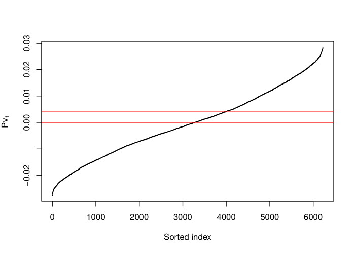
Figure 1: Example plot of the ordered entries of $v_{1}$ for the EisenYeast example from Section 4. The red lines illustrate the interval corresponding threshold $t=0.99$ placed at an arbitrary location on the vertical axis. Points farther apart than this interval correspond to column vectors that do not meet the correlation threshold.

Let $D^{i}\in\mathcal{R}^{n-i,n}$, $i=1,2,\ldots,n-1$, be the $i$th order finite difference matrix with $-1$ along the diagonal, $1$ along the $i$th super-diagonal, and zeros elsewhere. Then $D^{1}Pv_{1}$ consists of the differences of adjacent entries in $Pv_{1}$. Entries such that $\sigma_{1}^{2}(D^{1}Pv_{1})^{2}>2(1-t)$ correspond to pairs of vectors that do not meet the correlation threshold, where here and below an exponent applied to a vector denotes element-wise exponentiation.

Even a 1-d projected interval distance threshold may prune many possible non-adjacent vector pairs with respect to the ordering defined by $P$ as illustrated by the example in Figure 1. However, this observation is unlikely to rule out many adjacent pairs of vectors in most problems. For instance, the maximum distance between adjacent points shown in the example in Figure 1 is less than $\sqrt{2(1-t)}/\sigma_{1}$, and no pruning of adjacent pairs of vectors with respect to the ordering $P$ occurs.

Including more terms from Equation 2 increases our ability to prune adjacent pairs of vectors below the correlation threshold with respect to the ordering defined by $P$. Including only one more term finds that 96% of adjacent vectors fall below the correlation threshold of $0.99$ in the example shown in Figure 1 and are pruned by identifying indices such that

$$\sigma_{1}^{2}(D^{1}Pv_{1})^{2}+\sigma_{2}^{2}(D^{1}Pv_{2})^{2}>2(1-t).$$

Note that we use the permutation $P$ defined by the order of vector $v_{1}$ throughout. In general, using $p\leq k$ terms to prune pairs of vectors below the correlation threshold boils down to evaluating the expression

$$(D^{1}PV_{1:p})^{2}s_{1:p}^{2}>2(1-t),$$ (3)

where $V_{1:p}$ denotes the first $p$ columns of the matrix $V$, $s_{1:p}$ the vector of the first $p$ singular values.

Let $\ell$ be the longest run of successive points in $Pv_{1}$ within the interval $\sqrt{2(1-t)}/\sigma_{1}$. The quantity $\ell$ may, for example, be obtained by rolling the interval over all the points in Figure 1 and counting the maximum number of points that lie within the interval. With respect to the ordering $P$, $\ell$ represents the biggest index difference that pairs of indices corresponding to correlated vectors above the threshold can exhibit.

Pairs of vectors below the correlation threshold that lie more than one index difference apart relative to the permutation $P$ can be similarly pruned by replacing $D^{1}$ with $D^{j}$, $j=2,3,\ldots,\ell$ in the above expressions. Following this process, we can produce a well-pruned candidate set of vector pairs that contains all pairs that meet a given correlation threshold using $\ell$ matrix vector products with matrices of order $n\times p$, where $p$ is chosen in practice such that $p<<k$. Setting $p=10$ for the example shown in Figure 1 with $t=0.99$ prunes all but $149$ possible vector pairs out of a total $6221(6221-1)/2=19,347,310$ with $\ell=787$.

These steps are formalized in Algorithm 1 below. The algorithm proceeds in two main parts: steps 1–6 prune pairs of vectors down to a small candidate set that may meet the correlation threshold; step 7 computes the correlation values and applies the threshold across the reduced set of vector pairs.

Algorithm 2.1
Input: data matrix $A\in\mathcal{R}^{m\times n}$ with columns scaled to have zero mean and unit norm, correlation threshold $t$, truncated SVD rank $p<<k$.

1. Compute the truncated SVD $AV_{1:p}=U_{1:p}\mathrm{diag}(s_{1:p})$, where
   $V_{1:p}=[v_{1},v_{2},\ldots,v_{p}]$ and $\mathrm{diag}(s_{1:p})$ denotes the diagonal matrix of the first $p$ singular values.

2. Compute permutation $P$ that orders points in $v_{1}$.

3. Compute $\ell$, the longest run of successive points in $Pv_{1}$ within the interval $\sqrt{2(1-t)}/\sigma_{1}$.

4. Compute a set of candidate index pairs $(\tilde{j},\tilde{j}+\tilde{i})$ with respect to the index order defined by the permutation $P$ that possibly meet the correlation threshold

   $$\bigcup_{\tilde{i}=1}^{\ell}\left\{(\tilde{j},\tilde{j}+\tilde{i}):e_{\tilde{j}}^{T}(D^{\tilde{i}}PV_{1:p})^{2}s_{1:p}^{2}\leq 2(1-t)\right\},$$

   where $\tilde{j}=1,2,\ldots,n-\tilde{i}$.

5. If there are judged to be “too many” candidate pairs, increase $p$, compute $AV_{1:p}=U_{1:p}\mathrm{diag}(s_{1:p})$ and go to step 4. Continue to increase $p$ in this way until the number of candidate pairs is sufficiently small or stops decreasing (the best this algorithm can do).

6. Recover the non-permuted candidate column vector indices $(j,i)$ from $j=e_{\tilde{j}}^{T}Pq$ and $i=e_{\tilde{j}+\tilde{i}}^{T}Pq$ for every pair $(\tilde{j},\tilde{j}+\tilde{i})$ in step 4, where $q\in\mathcal{R}^{n}=[1,2,\ldots,n]^{T}$.

7. Compute the full correlation coefficient for each column vector pair identified in the previous step, applying the correlation threshold to this reduced set of values.

One can cheaply estimate whether there are “too many” candidate pairs for a given dimension $p$ in step 5 by evaluating step 4 for only adjacent pairs of vectors, $\tilde{i}=1$.

Algorithm 1 guarantees that no pruned vector pair exceeds the given correlation threshold–the pruning does not produce false negatives. The algorithm typically prunes the vast majority of pairs of vectors below the correlation threshold with truncated singular value decompositions of only relatively low rank $p$. The choice of $p$ represents a balance between work in computing a truncated SVD and evaluating $\ell$ rank $p$ matrix products in Step 4 (each increasing in work as $p$ increases), and the work required to filter the thresholded values in step 7 (decreasing work as $p$ increases).

Most of the floating point operations occur in step 4 of Algorithm 1. Fortunately the $\ell$ evaluations in step 4 are independent of each other and can easily be computed in parallel. See the reference R implementation [10] for an example.

3 General matrices and fast truncated SVD

We have so far assumed that the mean of each column vector of the $m\times n$ matrix $A$ is zero and the columns are scaled to have unit norm, but we really want a method that works with general matrices $A$. We also want a way to efficiently compute a relatively low-rank truncated SVD of potentially large matrices required by step 1 of Algorithm 1. And the truncated SVD method should be able to cheaply restart to compute additional singular vectors as required in step 5 of Algorithm 1. Fortunately all desires are met by one algorithm.

The augmented implicitly restarted Lanczos bidiagonalization algorithm(IRLBA) of Baglama and Reichel [2] efficiently computes truncated singular value decompositions of large dense or sparse matrices. Reference implementations are available for R [3], Matlab [1], and Python [8].

We can relax the column mean and scale assumptions without introducing much additional computational or storage overhead as follows. Assume $A$ is an $m\times n$ real-valued matrix without any constant-valued columns. Let $z=[z_{1},z_{2},\ldots,z_{n}]\in\mathcal{R}^{n}$ represent the vector of column means of $A$, $w=[w_{1}^{2},w_{2}^{2},\ldots,w_{n}^{2}]\in\mathcal{R}^{n}$ be the vector of squared column norms of $A$, and $W\in\mathcal{R}^{n\times n}$ a diagonal matrix with diagonal entries $1/\sqrt{w_{i}^{2}-mz_{i}^{2}}$. Let $e\in\mathcal{R}^{m}$ be a vector of all ones. Then $(A-ez^{T})W$ is a centered matrix with zero column means and scaled to have unit column norms, and

$$\mathrm{cor}(A)=W^{T}(A-ez^{T})^{T}(A-ez^{T})W.$$

The IRLBA, based on the Lanczos process, is a method of iterated matrix-vector products. The main idea behind efficient application of IRLB to correlation problems replaces matrix-vector products of the form $Ax$ with $AWx-ez^{T}Wx$ in the iterations, implicitly working with a scaled and centered matrix without forming it. This comes at the cost of storing two additional length $n$ vectors and at most computing two additional vector inner products per matrix-vector product. The R implementation [3] of IRLBA includes arguments for centering and scaling the input matrix.

A naïve brute force thresholded correlation computation requires $O(n^{2}m)$ flops. Let $p$ be the selected IRLBA dimension. Then Algorithm 1 requires $O(np\ell)$ flops, where $\ell$ is the longest run of ordered entries in $v_{1}$ that meet the 1-d projected distance threshold $\sqrt{2(1-t)}/\sigma_{1}$, including the flops required by IRLBA and final thresholding in step 7. The main computational savings of $\frac{nm}{lp}$ depends on the rate of decay in the singular values of $A$, the subspace dimension $p$, and the desired threshold value. We remark that this estimate of computational savings is available already in step 3 of Algorithm 1 after only modest computational effort. Users might use this cheap estimate to, for example, alter their threshold in some cases.

4 Numerical experiments

We evaluated the algorithm using public gene expression and DNA methylation datasets from the R biclust [7] package and from the Cancer Genome Atlas [4], referred to as TCGA. Most tests were performed on a desktop PC with a single AMD A10-7850K 3.7 GHz Athlon quad-core CPU and 16 GB 1333 MHz unbuffered RAM running the Ubuntu 15.10 GNU/Linux OS. Tests were performed with 64-bit R version 3.2.3 using double-precision arithmetic and the OpenBLAS library version 0.2.14-1ubuntu1 (based on Goto’s BLAS version 1.13) with OMP_NUM_THREADS=1. The last experiment includes a test run on a Linux cluster described in that section.

All examples use the reference R implementation, tcor(), which can be installed from the development GitHub repository using the devtools package with:

> devtools::install_github("bwlewis/tcor")

The native R cor() function is a general function that can compute several different types of correlation matrices including Pearson, Spearman, and Kendall and includes a number of options for dealing with missing values. Because of its flexibility, the native cor() function does not always compute Pearson correlation matrices in the most computationally-efficient way.

Correlation matrix computation can benefit substantially from use of optimized BLAS Level 3 operations (matrix multiplication), achieving high utilization of available CPU floating point capacity. The tcor() function also benefits from optimized BLAS routines, but not as much, as it mostly makes use of Level 2 operations and Level 3 operations on sequences of smaller problems.

We compare the tcor() function with brute-force Pearson correlation matrix computation computed in the fastest way we can, directly using matrix multiplication instead of using the more general cor() function.

4.1 Small gene expression example

The first example is a small proof of concept that provides the data for Figure 1 and establishes our timing and memory use measurement methodology. Wall-clock times are reported in seconds and peak memory use in excess of memory required to store the input data matrix is reported in megabytes.

Anyone can quickly run the example to experiment with the algorithm and compare its output with brute force results. The example uses the EisenYeast data from the biclust R package [7]. The data consist of 80 experiments involving the Saccharomyces Cerevisiae yeast measuring gene expression data across 6,221 Affymetrix probes, represented as an $80\times 6221$ real-valued matrix. The example finds all pairs of columns (gene expression measurements) that meet or exceed a Pearson correlation value of 0.95. The choice of projection dimension $p$ affects the efficiency of the algorithm. For $p=2$ the number of candidate vector pairs generated in step 4 of Algorithm 1 is over 3 million. When $p$ is increased to $10$, the number of candidate vector pairs drops to less than 13,000. The reference R implementation includes options for tuning $p$ and relies on the restart ability of the IRLBA to pick up where it left off and inexpensively extend an existing truncated SVD. The following example uses $p=10$.

> threshold = 0.95> # Test system values:> t1=3.13> t2=1.75> m1=59.60> m2=1075.10> if(Sys.getenv("RUN_EXAMPLES")=="TRUE")+ {+ library(tcor)+ library(doMC)     # local parallel computation+ library(biclust)  # for the BicatYeast data+ data(EisenYeast)  # in gene by sample orientation+ A = t(EisenYeast) # to correlate genes to genes+ # Register a four-core multicore parallel backend+ registerDoMC(4)++ # Compute using tcor():+ m1  = sum(gc()[,2])  # Memory in megabytes currently in use+ t1  = proc.time()+ tx  = tcor(A, t=threshold, p=10)+ t1  = (proc.time() - t1)[3] # Time in seconds+ m1  = sum(gc()[,6]) - m1    # Peak excess memory use during the test++ # Fast brute force full correlation:+ m2  = sum(gc()[,2])+ t2  = proc.time()+ mu = colMeans(A)+ s  = sqrt(apply(A, 2, crossprod) - nrow(A) * mu ^ 2)+ cs = scale(A, center=mu, scale=s)  # scale and center the data+ cx = crossprod(cs)                 # full correlation matrix+ cx  = cx * upper.tri(cx)    # ignore symmetry and diagonal+ pairs = which(cx >= threshold, arr.ind=TRUE)+ t2  = (proc.time() - t2)[3]+ m2  = sum(gc()[,6]) - m2+ } Brute-force computation outperforms tcor() in this small first example in speed but consumes substantially more memory. Each algorithm identifies the same set of 125 gene expression pairs that exceed the specified correlation threshold of 0.95, with comparative timing and memory use shown in the following table.

Method	Wall clock time (s)	Peak excess memory use (MB)
tcor	3.13	59.60
brute force	1.75	1075.10

Table 1: Gene expression results, threshold=0.95

4.2 TCGA DNA methylation example

Performance benefits from the tcor() function become apparent with more data. The following example uses calculated beta values from the Illumina Human Methylation450 BeadChip of 80 Adenoid Cystic Carcinoma (ACC) tumor samples obtained from the Broad GDAC Cancer Genome Atlas dashboard [4]. See the R package implementation [10] for examples of efficiently converting the downloaded sample methylation data into an R matrix. We chose these data for their public availability as a general example of computing thresholded correlation among large numbers of vectors, rather than for any specific biological meaning.

We removed 91,563 columns with all constant or missing values from the data, leaving an $80\times 394014$ matrix. The example computes pairs of methylation beta value column vectors with correlation values of 0.99 or more. We used a tcor projection dimension of 10 and the same performance measurement methodology used in the first example. Despite its low rank and modest data size, the problem is too large to compute using a naïve brute force correlation method. (We remark that the matrix multiplication central to the brute force implementation can be decomposed into a sequence of smaller steps to fit within given memory constraints. However, the brute force algorithm would still need to evaluate all possible vector pair correlation values.)

Algorithm 1 identified 913,601 pairs of vectors with correlation values of 0.99 or more in about three hours on our test PC. A brute force algorithm would need to evaluate the threshold condition for more than 77 billion vector pairs; the projection of Algorithm 1 limited the search space to only about 4 million candidate pairs, from which the 913,601 correlated pairs were found.

We illustrate that steps 4–7 of Algorithm 1 can be computed in parallel by comparing the above results run on our reference test PC with results run on a modest GNU/Linux cluster at Paradigm4, Inc. The cluster consisted of four computers connected by 10 gigabit ethernet. Each computer contained two Intel Xeon E5-2650 2 GHz CPUs (16 physical CPU cores per computer) and 64 GB/1,600 MHz ECC registered RAM running CentOS 6.6 and 64-bit R version 3.2.2 with the reference R BLAS library.

No code change was required to run in parallel on the cluster. The reference R tcor() implementation uses R’s foreach [12] framework to run on arbitrary parallel configurations (“back ends”). We simply registered a doRedis [9] parallel back end with 16 R workers per computer (64 total R worker processes) prior to invoking tcor().

The results computed on the Linux cluster are marked “tcor (64 core cluster)” below. The cluster example computed the filtering step 7 of Algorithm 1 in parallel across the 64 remote R processes. That approach incurs, in this example, an additional memory overhead of about 16 GB because each remote R process requires access to a copy of the data matrix $A$. More thrifty adaptations of the algorithm are possible and could, for example, share the memory required by $A$ between worker R processes on each computer.

Method	Wall clock time (s)	Memory use (MB)
tcor (4 core PC)	10309.00	389.10
tcor (64 core cluster)	482.00	994.30	(local)
		42282.40	(remote)

Table 2: TCGA ACC Methylation450 (80 rows x 394,014 columns, threshold=0.99). Linux cluster results include master R process memory use (local) plus total peak memory used by all 64 worker R processes (remote).

From a set of almost 80 billion pairs of vectors, Algorithm 1 finds 913,601 pairs with correlation values of 0.99 or more on a modest Linux cluster in about 8 minutes. The same algorithm works, more slowly, in the constrained memory setting of a desktop PC without modification.

5 Extensions

The idea of evaluating threshold conditions by projection into low dimensional subspaces applies to distance metrics similarly to correlation, see [14] for a related approach. Lemma 1.2 decomposes Euclidean distance between two vectors in terms of singular basis vectors and Algorithm 1 can be applied directly to the problem of finding all pairs of vectors that meet a thresholded Euclidean distance with small changes in steps 3, 4, and 7. By equivalence of norms, thresholded Euclidean distance can be extended to other distance metrics. The reference R implementation [10] includes functions for thresholded distance and correlation.

The ideas presented here can be adapted to efficiently find the top N most correlated vector pairs for a given constant N similarly to the work of Xiong et al. [15].

6 Conclusion

We present a simple algorithm and reference R implementation based on a truncated singular value decomposition (SVD) that efficiently computes thresholded subsets of large correlation matrices. We show that the natural connection between data covariance and the SVD can result in substantial computational and memory savings, and illustrate these savings with a few genomics data experiments. The main computational work in the algorithm is easily parallelized and deployed across computational clusters.

References

- [1] James Baglama. Irlba matlab code, 2005.
- [2] James Baglama and Lothar Reichel. Augmented implicitly restarted lanczos bidiagonalization methods. SIAM Journal on Scientific Computing, 27.1:19–42, 2005.
- [3] Jim Baglama and Lothar Reichel. irlba: Fast Truncated SVD, PCA and Symmetric Eigendecomposition for Large Dense and Sparse Matrices, 2015. R package version 2.0.0.
- [4] Broad Institute TCGA Genome Data Analysis Center. Analysis-ready standardized tcga data from broad gdac firehose stddata 2015-06-01 run, 2015. Dataset.
- [5] Mark A. Hall. Correlation-based feature selection for machine learning. PhD thesis, The University of Waikato, 1999.
- [6] Alfred Hero and Bala Rajaratnam. Large-scale correlation screening. Journal of the American Statistical Association, 106(496):1540–1552, 2011.
- [7] Sebastian Kaiser, Rodrigo Santamaria, Roberto Theron, Luis Quintales, and Friedrich Leisch. biclust: BiCluster Algorithms, 2015. R package version 1.2.0.
- [8] Michael Kane and Bryan Lewis. IRLBA Python module, 2014.
- [9] B. W. Lewis. doRedis: Foreach parallel adapter for the rredis package, 2014. R package version 1.1.1.
- [10] B. W. Lewis, James Baglama, Michael Kane, and Alex Poliakov. tcor: Fast Thresholded Correlation and Distance Matrices, 2015. R package version 0.0.0.
- [11] Abdullah Mueen, Suman Nath, and Jie Liu. Fast approximate correlation for massive time-series data. In Proceedings of the 2010 ACM SIGMOD International Conference on Management of data, pages 171–182. ACM, 2010.
- [12] Revolution Analytics and Steve Weston. foreach: Provides foreach looping construct for r, 2015. R package version 1.4.3.
- [13] Lin Song, Peter Langfelder, and Steve Horvath. Comparison of co-expression measures: mutual information, correlation, and model based indices. BMC bioinformatics, 13(1):328, 2012.
- [14] Daniel Wu, Ambuj Singh, Divyakant Agrawal, Amr El Abbadi, and Terence R Smith. Efficient retrieval for browsing large image databases. In Proceedings of the fifth international conference on Information and knowledge management, pages 11–18. ACM, 1996.
- [15] Hui Xiong, Mark Brodie, and Sheng Ma. Top-cop: Mining top-k strongly correlated pairs in large databases. In Data Mining, 2006. ICDM’06. Sixth International Conference on, pages 1162–1166. IEEE, 2006.
- [16] Hui Xiong, Shashi Shekhar, Pang-Ning Tan, and Vipin Kumar. Taper: A two-step approach for all-strong-pairs correlation query in large databases. Knowledge and Data Engineering, IEEE Transactions on, 18(4):493–508, 2006.
- [17] Lei Yu and Huan Liu. Feature selection for high-dimensional data: A fast correlation-based filter solution. In ICML, volume 3, pages 856–863, 2003.
- [18] Jian Zhang and Joan Feigenbaum. Finding highly correlated pairs efficiently with powerful pruning. In Proceedings of the 15th ACM international conference on Information and knowledge management, pages 152–161. ACM, 2006.