Image Reconstruction Image reconstruction by using local inverse for full field of view.

Abstract

The iterative refinement method (IRM) has been very successfully applied in many different fields for examples the modern quantum chemical calculation and CT image reconstruction. It is proved that the refinement method can create a exact inverse from an approximate inverse with a few iterations. The IRM has been used in CT image reconstruction to lower the radiation dose. The IRM utilize the errors between the original measured data and the recalculated data to correct the reconstructed images. However if it is not smooth inside the object, there often is an over-correction along the boundary of the organs in the reconstructed images. The over-correction increase the noises especially on the edges inside the image. One solution to reduce the above mentioned noises is using some kind of filters. Filtering the noise before/after/between the image reconstruction processing. However filtering the noises also means reduce the resolution of the reconstructed images. The filtered image is often applied to the image automation for examples image segmentation or image registration but diagnosis. For diagnosis, doctor would prefer the original images without filtering process.

In the time these authors of this manuscript did the work of interior image reconstruction with local inverse method, they noticed that the local inverse method does not only reduced the truncation artifacts but also reduced the artifacts and noise introduced from filtered back-projection method without truncation. This discovery lead them to develop the sub-regional iterative refinement (SIRM) image reconstruction method. The SIRM did good job to reduce the artifacts and noises in the reconstructed images.

The SIRM divide the image to many small sub-regions. To each small sub-region the principle of local inverse method is applied. After the image reconstruction, the reconstructed image has grids on the border of sub-region inside the object. If do not consider the grids, the noise and artifacts are reduced compare the original reconstructed image. To eliminate the grids, these authors have to add the margin to the sub-region. they did not think the margin is important issue in the beginning. However when they considering the size of sub-region tending to only one pixel, they found that the margin play a important role. This limit situation of sub-regional iterative refinement is referred as local-region regional iterative refinement(LIRM). If the margin is very large for example as half the image size, the SIRM and the LIRM become no iterative refinement method (NIRM), i.e. normal filtered back-projection method. If the size of the margin tend to 0, the LIRM become the IRM, which is also referred as traditional iterative refinement method (TIRM). For SIRM and LIRM, if margin is too small, the image is rich in noise like IRM, if the margin is too big the image is rich in artifacts like NIRM. If a suitable margin is taken, for example the margin is around 20 pixel for a 512*512 image, the summation of the noise and artifacts can be minimized.

SIRM and LIRM can be seen as local inverse applied to the image reconstruction of full field of veiw. SIRM and LIRM can be seen as generalized iterative refinement method(GIRM). SIRM and LIRM do not minimize the noise or artifacts but minimize the summation of the noise and artifacts. Even the SIRM and LIRM are developed in the field of CT image reconstruction, these authors believe they are a general methods and can be applied widely in physics and applied mathematics.

¹Imrecons.com North York, Ontario, Canada

²Northwestern Poly Technical University Xi’an China

Keyword: artifact, noise, Local, inverse, iteration, iterative, reprojection, image reconstruction, filtered back-projection, FBP, x-ray, CT, parallel-beam, fan-beam, cone-beam, sub-regional, local-region, iterative refinement, LFOV, ROI, Tomography, filter

1 Introduction

1.1 Iterative refinement method (IRM) in applied mathematics, physics and image recovery / image reconstruction

The IRM[1] is widely applied to physics and applied mathematics for example ref.[32, 33]. The advantage of the IRM is that it can produce an exact inverse from approximate inverse[37, 38]. A recent very important application of the IRM in quantum physics can be found[35] in which the Eigen values can be calculated dependent linearly with the size of matrix. The IRM is also applied to image recovery[36] and MR image reconstruction[34].

1.2 IRM in CT image reconstruction

Many reconstruction algorithms have been developed for parallel-beam[2], fan-beam[8, 9, 2, 11, 22, 23], and cone-beam tomographic systems[18, 19, 20, 21, 24]. The above reconstruction methods which has no iteration are referred as direct reconstruction. On the other hand, image can be reconstructed by IRMs[3, 4, 5, 6, 7]. In the IRM, the reconstructed image is re-projected and the errors between the measured projections and re-projections are calculated. These errors are utilized to correct the first reconstruction. In order to distinguish other IRM which will be introduced later in this article, this IRM is referred as traditional iterative refinement reconstruction method (TIRM). The direct reconstruction without iterative refinement is referred as non iterative refinement reconstruction method (NIRM). The TIRM is known that it can reduce artifacts especially beam-harden artifacts at a price of increasing the noises. Moreover, TIRM is more time-consuming compared to the direct reconstruction (NIRM), since it has a iteration. Time-consuming in image reconstruction is not a big issue in our generation since the improvement of the computer hardware. A recent iterative refinement reconstruction was the work of Johan Sunnegardh[10]. Siemens AG has claimed that Johan’s method is their new generation CT image reconstruction method. This means that big companies begin to notice the importance of the IRM in image reconstruction. It is noticed that Johan’s iterative refinement reconstruction has a pre-filtering and post-filtering process which are used to reduce the noises of their IRM. For CT image reconstruction the IRM can reduce the artifacts of reconstructed image hence reduce the dose required for CT image. However the IRM often has an over-corrections on the image edges which increases the noises. Johan’s iterative refinement reconstruction has to include filtering process to reduce the noises. Pre-filtering and post-filtering process does not only reduce the noises, but it also decreases the information contained in the original projection data. these authors have also roughly introduced a IRM in the past which is referred as sub-regional iterative refinement method (SIRM)[31]. SIRM dose not include pre-fltering and post filtering processes, since their noise level is not increased. This article offers the details and also the history how this method has been discovered. The limit situation when the size of the sub-region approaches to $1$ is also discussed, in this case the SIRM method becomes local-region iterative refinement method (LIRM).

1.3 The history about developing the SIRM and LIRM

One of the important task in image reconstruction is to reduce the truncation artifacts. The truncation artifacts are caused by LFOV (limited field of view) of the detector. The truncation artifacts can be reduced through extrapolation of the missing rays[13, 17, 12] or local tomography[16, 17, 25, 26, 12]. Extrapolation often produces an over-correction or an under-correction to the reconstructed image[30]. Local tomography cups the reconstructed image. Iterative reconstruction and re-projection algorithm [14, 15, 27] was developed for the reconstruction of limited angle of view. Another iterative reconstruction re-projection algorithm has been developed for LFOV[28]. The iterative algorithm for LFOV reduces the truncation artifacts remarkably. This algorithm led to a truncation free solution local inverse for LFOV[30]. The fast extrapolation used in [30] is done in [29]. During the work with the iterative algorithm for LFOV, it was occasionally found that this algorithm did not only reduce the truncation artifacts but also it reduced the normal artifacts. Here the normal artifacts means that the artifacts exist in the direct reconstruction (NIRM) for example FBP (filtered back projection) method with full field of view (FFOV). It is well know that even FBP method is a exact method, it is actually not exact because the numerical calculations. This finding led to the SIRM for FFOV[31].

SIRM was adjusted to suit the case of FFOV. This was done by taking away the extrapolation process. The first reconstruction in the iteration was FBP method. For the second reconstruction, the region of the object was divided to many sub-regions. The iterative reconstruction was done for each sub-region adding a margin. The part of the object from the 1st reconstruction outside a sub-region (including its margin) was reprojected. These re-projections were subtracted from the original projections. The resulted projections were utilized to make the second reconstruction inside the sub-region. Finally the reconstructed images on all sub-regions were put together. It is worthwhile to say that the margin was added in the beginning to eliminate the cracks on the border of the sub-regions. It was not thought as an important issue. However it was found that it was the margin that really plays the role to reduce artifacts [31] and decreasing the noises.

1.4 Other image reconstruction methods

It is worth to mention that Many fanbeam and conebeam image reconstruction algorithms have been derived in recent 20 years. Amongst these derivations are the following examples: the references[40, 41, 42, 43, 57, 60, 62, 66, 80, 81, 28, 29, 30, 31] are reconstruction algorithms for truncated projections, super short scan, interior and exterior reconstruction. The references[44, 74, 75] are reconstruction algorithms in Fourier domain. The references[46, 47, 49, 58, 67, 69, 70, 72, 76] are reconstruction algorithms with FBP method. The references[53, 64, 65, 82] are reconstruction algorithms with total variation (TV) minimization or compressed sensing method. The references[52, 54, 56, 68] are reconstruction algorithms with iterations. The references[50, 63] are reconstruction algorithms with GPU accelerate. The reference[45] is reconstruction with neural network algorithm. The reference[48] is the reconstruction algorithm with multiresolution. The reference[59] is reconstruction with dual-source. The reference[79] introduces the reconstruction with a Laplace operator. The extrapolation method[87, 88, 12] and adapted extrapolation method[83, 84, 85, 86] to solve LFOV problem.

1.5 These author’s contributions

Two generalized iterative refinement methods (IRM), i.e. sub-regional iterative refinement method (SIRM) and local-region iterative refinement method (LIRM) for inverse problem or CT image reconstruction with FFOV are introduced, which can reduce the artifacts and keep the noise not increased too much. In SIRM the reconstructed image has been divided to small pieces and re-projected, reconstructed to produce the final reconstruction image. SIRM was used to overcome the problem of the TIRM (i.e. the artifacts reduction is at the price of increasing the noises).

Among NIRM, TIRM, LIRM and SIRM. there are two parameters which are the margin size of the sub-region and the size of sub-region. The margin size is originally introduced to eliminate the grids on the reconstructed image of the SIRM. These authors found that if the margin size is between 0 and the size of image and the sub-region is chosen as small as one pixel (the size of sub-region equals 1), the SIRM becomes LIRM. If the margin size also closes to 0 then the LIRM becomes TIRM. If the margin size is large enough such as same size of image, the LIRM becomes NIRM. Hence, the relationship among the SIRM, LIRM, TIRM and NIRM are summarized. These authors have proved that LIRM is a special situation of SIRM and proved that NIRM and TIRM are special situation of LIRM. Hence LIRM and SIRM are two generalized IRM.

The examples of LIRM in simple inverse problem is introduced to learn the concept of LIRM, which are also suitable to SIRM. these authors did not implement LIRM for CT image reconstruction, since it is very time consuming. A CT reconstruction example using SIRM is done.

1.6 Arrangement in this article

In section 2 these authors review the reconstruction method without iterative refinement (NIRM). In section 3 TIRM is discussed. In section 4 LIRM is discussed . In section 5 the SIRM is discussed.

2 Local inverse to solve under determinate equation

Assume the determinate equation is

$$T\,z=h$$

where $T$ is a $m\times m$ matrix, $z$ is a unknown vector with length $m$. $z\in Z$ $h$ is a known vector of length $m$. $h\in H$. $Z$ and $H$ are definite region of $z$ and $h$. Assume

$$T=\left[\begin{array}[]{cc}A&B\\ C&D\end{array}\right]$$

$A$, $B$, $C$, $D$ are submatrix of $T$,

$$h=\left[\begin{array}[]{c}f\\ g\end{array}\right]$$

$$z=\left[\begin{array}[]{c}x\\ y\end{array}\right]$$

$f$ and $g$ are subvector of $h$. $x$ and $y$ are subvector of $z$. We assume $x\in X$, $y\in Y$. Here $X+Y=Z$. We assume $X$ is the interior region or region of interest (ROI). $Y$ is the outside region or outer side of ROI. We assume $f\in F$, $g\in G$, $G+F=H$. $F$ is called field of view (FOV). $G$ is called outside of FOV.

$$\left[\begin{array}[]{cc}A&B\\ C&D\end{array}\right]\left[\begin{array}[]{c}x\\ y\end{array}\right]=\left[\begin{array}[]{c}f\\ g\end{array}\right]$$

In the case only $f$ is known, the above equation can be written as

$$\left[\begin{array}[]{cc}A&B\end{array}\right]\left[\begin{array}[]{c}x\\ y\end{array}\right]=f$$

This is referred to under determinate equation which has infinite solution. One of the important solution is minimal norm solution.

$$\left[\begin{array}[]{c}x^{(0)}\\ y^{(0)}\end{array}\right]=\left[\begin{array}[]{cc}A&B\end{array}\right]^{+}f$$

The subscript “⁺” means generalized inverse which gives the the solution corresponding to minimal norm solution. subscript “⁽⁰⁾” corresponding to the solution of first iteration.

The minimal normal solution is not the best solution. The following we try to further improve the result with so called local inverse method.

Assume we are more interest to know “$x$”. We can subtract the contribution of $y^{(0)}$from $f$,

$$f^{(0)}=f-B\,y^{(0)}$$

We can calculate the solution $x^{(1)}$ the following way,

$$x^{(1)}=A^{+}f^{(0)}$$

We found that the above solution has no any improvement, i.e.

$$x^{(1)}=x^{(0)}$$

However we can change the formula of $f^{(0)}$ to

$$f^{(0)}=f-B\,\mathrm{modify}(y^{(0)})$$

The above function “$\mathrm{modify}$” is just modify the mean value or flop according some priori. In this way we can improve the result a lot. The following is a example.

The local inverse is introduced with very simple example. Assume

$$A=\left[\begin{array}[]{cccc}3&4&7&6\\ 8&5&8&7\\ 3&6&9&8\\ 4&2&8&9\end{array}\right]$$

$$B=\left[\begin{array}[]{cccc}4&5&6&7\\ 8&7&6&5\\ 6&3&4&6\\ 4&8&4&10\end{array}\right]$$

$$x=\left[\begin{array}[]{c}3\\ 4\\ 3\\ 6\end{array}\right]$$

$$y=\left[\begin{array}[]{c}2\\ 6\\ 4\\ 8\end{array}\right]$$

Assume

$$z=\left[\begin{array}[]{c}x\\ y\end{array}\right]$$

We can calculate

$$A\,x+B\,y=f$$

Now we assume we know vector $f$ and matrix $A$, $B$, we need to solve $x$ and $y$. We can solve it with least square method so that can be write as

$$z^{(0)}=[A+B]^{+}f$$

$$x^{(0)}=first4(z^{(0)})$$

$$y^{(0)}=last4(z^{(0)})$$

We can calculate the errors

$$error_{x}^{(0)}=\sum|x^{(0)}-x|$$

$$error_{y}^{(0)}=\sum|y^{(0)}-y|$$

$$f_{x}^{(0)}=f-B\,k_{y}\,y^{(0)}$$

$modified(y^{0})=k_{y}\,y^{(0)}$

$$f_{y}^{(0)}=f-B\,k_{x}\,x^{(0)}$$

$modified(x^{(0)})=k_{x}\,x^{(0)}$

$$x_{1}=A^{+}f_{x0}$$

$$y_{1}=B^{+}f_{y0}$$

$$error_{x}^{(1)}=\sum|x^{(1)}-x|$$

$$error_{y}^{(1)}=\sum|y^{(1)}-y|$$

3 Nor iterative refinement reconstruction method (NIRM)

Assume the parallel-beam projections are known as $p=p(\theta,u)$, where $\theta$ is projection angle and $u$ is the index of detector elements. Assume the projection operator $P$ is known, which is 2D Radon transform. Assume the non-iteration reconstruction operator $R$ is also known, which is for example FBP reconstruction. However, the object or original image $X_{o}(x)$ is unknown. Here $x$ is the coordinates of the image pixel. The forward equation of the problem can be write as

$$P\,X=p=p_{o}+p_{n}$$ (1)

where $X$ is the unknown image of the above equation. $p_{o}$ is projections without noises

$$p_{o}=P\,X_{o}$$ (2)

$p_{n}$ indicates noises in projections. The image can be reconstructed as

$$X^{(0)}=R\,p$$ (3)

$X^{(0)}$ is the first iteration of the reconstructed image using the reconstruction operator $R$. The superscripts $(0)$ indicates that $X^{(0)}$ is the first reconstruction in the iteration which will appear in the following paragraph. The above two formulas can be written as

$$X^{(0)}=J\,X=J\>X_{o}+R\>p_{n}$$ (4)

The first term of the right of the above equation is the signal dependent reconstructed image. The second term is noise dependent reconstructed image. In the above equation, $J$ is the projection-reconstruction operator which is defined as

$$J\equiv R\,P$$ (5)

where $x$ is the index of the image pixel before projection-reconstruction operation. $y$ is the index of pixel of the image after the projection-reconstruction operation. The operation of Eq.(5) is defined as

$$J\,X=\sum_{x}j(y,x)\,X(x)$$ (6)

Here $j(y,x)$ is the kernel of operator $J$. $J$ can be written as

$$J=\sum_{x}j(y,x)\,\bullet$$ (7)

Where “$\bullet$” is multiplication.

The identical operator is defined in the following

$$I=\sum_{x}\delta(y,x)\,\bullet$$ (8)

where

$$\delta(y,x)=\left\{\begin{array}[]{c}1\,\,\,\,\,\,\,\,\textrm{if}\,\,\,\,y=x\\ 0\,\,\,\,\,\,\,\,\,\,\,\,\,\,\,else\end{array}\right.$$ (9)

From the above definition there is,

$$\sum_{y}\>\delta(y,x)=1$$ (10)

In the ideal reconstruction the reconstructed image is same as the original image that means $J\rightarrow I$. “$\rightarrow$” is “close to”. $J$ should satisfy the unitary condition same as $I$

$$\sum_{y}j(y,x)=1$$ (11)

Assume $x^{\prime}$ is any pixel in the image. The above equation can be rewritten as

$$\sum_{y}\sum_{x}\>j(y,x)\>\delta(x-x^{\prime})=1$$ (12)

The above equation means that the delta function $\delta(x-x^{\prime})$ after projection and reconstruction operation and sum operation $\sum_{y}$, $1$ is obtained.

The unitary condition guarantees that the dc-composition is not changed after the operation $J=R\>P$. $j(y,x)$ is referred as the resolution function, $J$ is referred as the resolution operator. In the above situation it is the resolution function of NIRM. The error of NIRM is defined as

$$Err^{(0)}\equiv X^{(0)}-X_{o}=(J-I)\>X_{o}+R\>p_{n}$$ (13)

The first term is corresponding to artifacts of the method. The second term is corresponding to noises of the method. Since the resolution function $J$ is not an exact unitary operator $I$, even if the noises $p_{n}=0$, it is true according to Eq.(13) in general that

$$X^{(0)}\neq X_{o}$$ (14)

One of the problem of the image reconstruction is how to improve the results of the reconstruction $X^{(0)}$ to let the reconstructed image more close to the original object function $X_{o}$ ? This can be rephrased as to find an algorithm with its resolution function more close to $\delta(y,x)$ function than the resolution function of NIRM $j(x,y)$ in the same time the noise term does not increase heavily. The IRMs (TIRM, LIRM and SIRM) deals this problem in the following sections. These methods have different noise characters and computation complicity.

4 Traditional iterative refinement reconstruction method (TIRM)

In order to further improve the reconstruction results $X^{(0)}$, TIRM was proposed. TIRM is iterative algorithm with the reconstruction and re-projection processes. It was obtained in the same way as the IRM to solve linear equation with an inaccurate known inverse operator. It was used so many times in different fields and hence it is difficult to find all of the sources of it. A few examples can be seen [3, 4, 5, 6, 7]. The processes of TIRM is given in the following. The errors i.e. the differences between the projections $p$ and re-projections $P\,X^{(0)}$ are calculated: $Err=(p-P\,X^{(0)})$. The errors are utilized to correct the reconstruction $X^{(1)}=X^{(0)}+R\,Err$. The algorithm can be summarized in the following

$$X^{(1)}=X^{(0)}+R\,(p-P\,X^{(0)})$$ (15)

where $X^{(0)}$ is obtained in Eq.(3). Substituting Eq.(3) to the Eq.(15), considering Eq.(5) the above algorithm can be seen as a filtering algorithm

$$X^{(1)}=F_{TIRM}X^{(0)}$$ (16)

Where the filtering function is defined as

$$F_{TIRM}\equiv 2\,I-J$$ (17)

Considering Eq.(10, 11) the filtering function $F_{TIRM}$ satisfies the unitary condition

$$\sum_{y}f_{TIRM}(y,x)=1$$ (18)

$f_{TIRM}(y,x)$ is kernel function of operator $F_{TIRM}$. The results of TIRM and NIRM will be utilized as contrast to LIRM which will be discussed in the next paragraph. The resolution operator of TIRM is $F_{TIRM}\>J$, which is really more close to identical operator $I$ than the resolution operator of NIRM $J$ does. However TIRM is rarely directly applied to clinical situation since it is sensitive to noises. This can be seen by further modify the Eq.(15) using Eq.(1), Eq.(2) and Eq.(3)

$$X^{(1)}=F_{TIRM}\>J\>X_{o}+F_{TIRM}R\>p_{n}$$ (19)

Hence the errors

$$Err^{(1)}\equiv X^{(1)}-X_{o}=(F_{TIRM\>}J-I)\>X_{o}+F_{TIRM}R\>p_{n}$$ (20)

The first term of the above formula is a signal dependent image, which is referred to as artifacts. The second term of the formula is the noise dependent image. It can be compared the above formula with Eq.(13). Since normally $F_{TIRM}\>J$ is closer to $I$ than $J$, the first term $F_{TIRM}\>J\>X_{o}$ is closer to $X_{o}$ than $J\>X_{0}$ does. This means that TIRM can get a more accurate reconstruction corresponding the first term. However the second term $F_{TIRM}R\>p_{n}$ is normally larger than $R\>p_{n}$. This means the TIRM is more noise sensitive than NIRM.

Recently a modified TIRM by Johan can be found in reference[10]. In Johan’s iterative refinement reconstruction (JIRM), a pre-filtering process, and two regularization filtering processes are added to TIRM. Johan has compared the resolution of his method JIRM with NIRM, Johan’s result the Figure 5.7 of [10]. a) in Figure 5.7 of [10] shows the resolution function of NIRM. b) in Figure 5.7 of [10] shows the resolution function JIRM without pre-filtering. c) in Figure 5.7 of [10] shows the resolution function of JIRM with pre-filtering. It can be seen that in b) in Figure 5.7 of [10], there is a black ring surrounding the white dot. This black ring is called over-correction. Over-correction increases the resolution but it leads a noise increase too. Johan used the pre-filtering process to overcome the problem of over-correction and noises. He first pre-filtered the projection data and applied the filtered data to his reconstruction. It is well know that the pre-filtering process does not only smooth the noise data but also reduced the information contained in the data. This is why many doctor prefer to see the noise data than the smoothed data after a filtering process. Pre-filtering process often is not accepted. The following section will shows the method to overcome the problem of over-correction in TIRM.

5 Local-region iterative refinement reconstruction method (LIRM)

5.1 The method

In this section another IRM is defined which is a special case of next section. First two operators $K$ and $H$ are define as following

$$K\>X=\sum_{x}k(y,x)\>X(x)$$ (21)

$$H\>X=\sum_{x}h(y,x)\>X(x)$$ (22)

where

$$k(y,x)=\begin{cases}\begin{array}[]{cc}j(y,x)&\mathrm{if}\>|x-y|\leq r\\ 0&\mathrm{else}\end{array}\end{cases}$$ (23)

$$h(y,x)=\begin{cases}\begin{array}[]{cc}0&\mathrm{if}\>|x-y|<r\\ j(y,x)&\mathrm{else}\end{array}\end{cases}$$ (24)

where $r$ is a constant parameter. It defines a region $[y-r,y+r]$ close to $y.$ $r$ is called the margin size. The margin will be explained in next section. In this section it is assumed that the image is 1-dimensional. But the result is easy to extent to 2 or 3 dimensional situation. It is clear that there is the relation:

$$J=K+H$$ (25)

The Local-region iterative refinement method (LIRM) is defined as following,

$$X^{(1)}=\eta\>R\>p-R\>(P\>\Omega)\>X^{(0)})$$ (26)

where $\eta$ is a normalized parameter which will be decided later and the operator $\Omega$ is defined as:

$$\Omega(y,x)=\begin{cases}\begin{array}[]{cc}0&\mathrm{if}\>|x-y|\leq r\\ 1&\mathrm{else}\end{array}\end{cases}$$ (27)

In this article all operators are linear operator except the operator $\Omega$ which is a normal multiplication operator, i.e.:

$$(J\>\Omega)\>X=\sum_{x}(j(y,x)\>\Omega(y,x))\>X(x)$$ (28)

Considering Eq.(3) and Eq.(5), Eq.(26) can be rewritten as

$$X^{(1)}=\eta\>X^{(0)}-(J\>\Omega)\>X^{(0)}$$ (29)

considering

$$J\>\Omega=H$$ (30)

the LIRM can rewritten as

$$X^{(1)}=\eta\>X^{(0)}-H\>X^{(0)}$$ (31)

The above formula is rewritten as

$$X^{(1)}=F_{LIRM}X^{(0)}$$ (32)

where

$$F_{LIRM}=\eta\>I\>-H=\eta\>I-J+K$$ (33)

$F_{LIRM}$ is the filtering function of the LIRM. Because $J$ can implemented as $P\>R$, $K$ can be implemented as a small matrix when $r$ is small. That is why the right part of the above formula is easier to be implemented than the middle part of the formula. Similar to Eq. (18) $F_{LIRM}$ should meet the unitary condition:

$$\sum_{y}\sum_{x}f_{LIRM}(y,x)\>\delta(x-x^{\prime})=1$$ (34)

This unitary condition means that if the input is $\delta(x-x^{\prime})$, $x^{\prime}$ is any point in the image, the whole output of the filter $F_{LIRM}$ is $1$, since $F_{LIRM}$ should looks like $\delta(y,x)$ function. The above condition can be write as

$$\sum_{y}f_{LIRM}(y,x)=1$$ (35)

Considering Eq. (33 and 35) implies that

$$\eta\equiv\eta(x)=1+\sum_{y}h(y,x)=2-\sum_{y}k(y,x)$$ (36)

The LIRM Eq.(26) can be interpreted as following. The reconstructed image $X^{(0)}$ is re-projected except the vicinity of the pixel where the iterative Reconstruction is calculated $(J\>\Omega)\>X^{(0)}$. The measured projection is reconstructed with $R$, scaled a little to adjust the dc composition $\eta\>R\>p$. The difference of the above two projections are used to produced a reconstruction $(\eta\>R\>p-(J\>\Omega)\>X^{(0)})$. Inside of the vicinity, only the center point is kept, which is the pixel where the iterative method is done. Other pixel can be obtained in the same way. The LIRM always concerns in a local region, which is the vicinity of the pixel. Hence it is referred as the local region iterative refinement method.

5.2 In the limit case

In this article the discussed IRM are generalized inverse methods. CT image reconstruction can be seen as a example. It is easy to understand the principle of method to consider the object $X_{o}$ as one dimensional image. Assume $x\in[-\frac{L}{2},\frac{L}{2}]$ is the coordinates of the image pixel. Here $L$ is the number of pixels of the image. if $r\rightarrow L$, then according to Eq.(23, 24, 25 and 36) there are

$$K\rightarrow J,\quad H\rightarrow 0,\quad\eta\rightarrow 1$$ (37)

Considering the above formula and Eq.(33) there is

$$F_{LIRM}=\eta\>I\>-H\rightarrow I=F_{NIRM}$$ (38)

i.e. in this case there is LIRM $\rightarrow$NIRM.

if $r\rightarrow 0$, the similarly according to Eq.(23, 24, 25) there are

$$k(y,x)\rightarrow j(y,x)\delta(y,x)$$ (39)

That is

$$K\rightarrow j(y,y)\>I$$ (40)

considering Eq.(36), there is

$$\eta(x)\rightarrow 2-j(x,x)$$ (41)

and

$$\eta\>I-J+K\rightarrow(2-j(y,y))\>I-J+j(y,y)\>I=2\>I-J$$ (42)

Considering the above formula and Eq.(33) and Eq.(17), there is

$$F_{LIRM}\rightarrow F_{TIRM}$$ (43)

i.e. in this case LIRM $\rightarrow$TIRM. This means that the NIRM and TIRM are two special cases of LIRM as $r\rightarrow L$ or $r\rightarrow 0$.

5.3 A simple example

In following example, the original image is 1-dimensional for simplicity. CT reconstruction is not taken which is at least two dimension. Assume the forward operator is $P=T\>V$. Here $T$ is assumed as discrete Fourier transform. The inverse operator is taken as $R=T^{-1}$ , $T^{-1}$ is the inverse discrete Fourier transform. Assume the size of the image is $L=128$. The blurring operator $V$ is assumed as

$$V(x)=\frac{1}{[(\frac{x}{\alpha L})^{2}+\beta]^{\rho}}$$ (44)

where $\alpha=0.01$, $\beta=0.2$, $\rho=0.9$. In this example the resolution function

$$J=R\>P=T^{-1}\>T\>V=V$$ (45)

In this example $J(x,y)=J(x-y)=V(x-y)$. $F_{NIRM}$, $F_{TIRM}$ and $F_{LIRM}$ are summarized as $F_{a}$. Corresponding 3 IRMs can be written as following,

$$X^{(1)}=F_{a}\>J\>X_{o}+F_{a}R\>p_{n}$$ (46)

The error function can be written as,

$$Err_{a}^{(1)}\equiv X^{(1)}-X_{o}=(F_{a}\>J-I)\>X_{o}+F_{a}R\>p_{n}$$ (47)

Here $a$ is corresponding to NIRM, TIRM and LIRM, and $F_{a}$ has 3 format, $F_{NIRM}=I$, $F_{TIRM}=2\>I-J$, $F_{LIRM}=\eta\>I-J+K$ The noises and artifacts depends on the shape of the operator $F_{a}$

5.4 Advantages and disadvantages

In general, the errors of LIRM are less than TIRM meaning that

$$||Err_{LIRM}||\ll||Err_{TIRM}||$$ (48)

The noises of LIRM are less than TIRM meaning that

$$\sigma_{y}^{2}\{Err_{LIRM}\}\ll\sigma_{y}^{2}\{Err_{TIRM}\}$$ (49)

Here $\sigma_{y}^{2}$ is defined local variance as

$$\sigma_{y}^{2}\{X(x)\}=\frac{1}{N-1}\sum_{x\in\omega_{y}}(X(x)-E(X(x)))^{2}$$ (50)

Where $\omega_{y}$ is the local region close to $y$. $E$ is the local mean defined as

$$E_{y}\{X(x)\}=\frac{1}{N}\sum_{x\in\omega_{y}}X(x)$$ (51)

Where $N$ is number of pixel(voxel) inside the local region $\omega_{y}$. $N$ can be found experimentally. these authors are not going to prove the above formula Eq(48, 49), instead an example in following section will show the results.

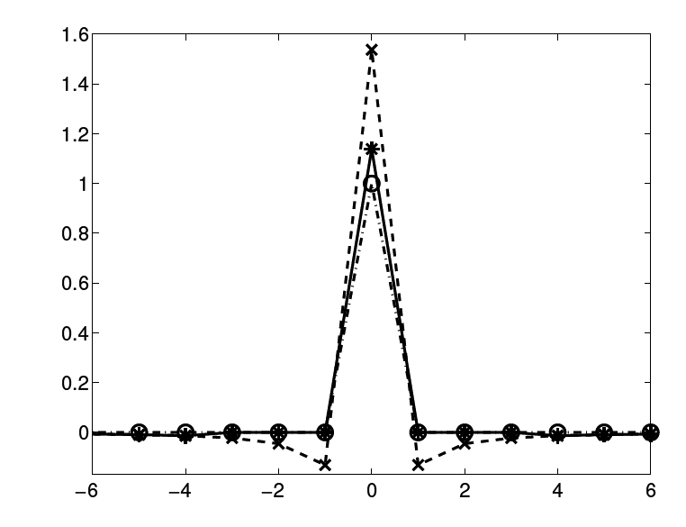
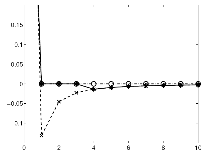
Figure 1: (a) The dash-dotted line with circle mark shows $F_{NIRM}(x)$, The dashed line with cross mark shows $F_{TIRM}(x)$, the solid line with star mark shows $F_{LIRM}(x)$. (b) is the zoomed image of (a) to see the vicinity at x=r. Here r=3. It is clear that there is a large negative values for $F_{TIRM}$ at $r=\pm 1.$

Figure 1 shows the filtering function of $F_{a}$ for different methods. I is can be seen that $F_{TIRM}$ has a large negative values at $|x|<r$. This is corresponding the black ring of the resolution function in b) of Figure 5.7 of the reference[10]. This is also referred as over-correction. The over-correction can increase the resolution yet it also increases the noises. On the other hand, the filtering function $F_{LIRM}$ has no large negative value at $|x|<r$. When $|x|>r$ $F_{LIRM}\simeq F_{TIRM}$ , hence $F_{LIRM}$ can also reduce the artifacts for example beam harden artifacts in CT reconstruction. In Figure 1 these authors choose $r=3$. $r$ is a parameter can be adjusted according to the size of the image. Usually the large the image size, the large the $r$ should be. From Figure 1 it can be seen that if $r\rightarrow 0$, there is $F_{LIRM}\rightarrow F_{TIRM}$. When $r\rightarrow L$, there is $F_{LIRM}\rightarrow F_{NIRM}$.

In the following it is assumed that $X_{o}(x)=\mathrm{sign}(x)$. The image edge is at the place $x=0$. It is also assumed that the size of image is $L=2048$, and $r=122$. Here these authors have increased the size of image to show the results more clearly. Measured data is simulated with $p_{o}=P\>X_{o}$. Matlab is used to created the simulated noise: $p_{n}(x)=0.004*randint(1,$[-5,5]). Noise $p_{n}$ is added to data $p=p_{o}+p_{n}$. Assume the forward operator is $P=T\>V$ . Here $T$ is assumed as discrete Fourier transform. The inverse operator is taken as $R=T^{-1}$ , $T^{-1}$ is the inverse discrete Fourier transform. $V$ is defined in Eq.(44). The three reconstruction results using the methods NIRM, TIRM, LIRM are compared.

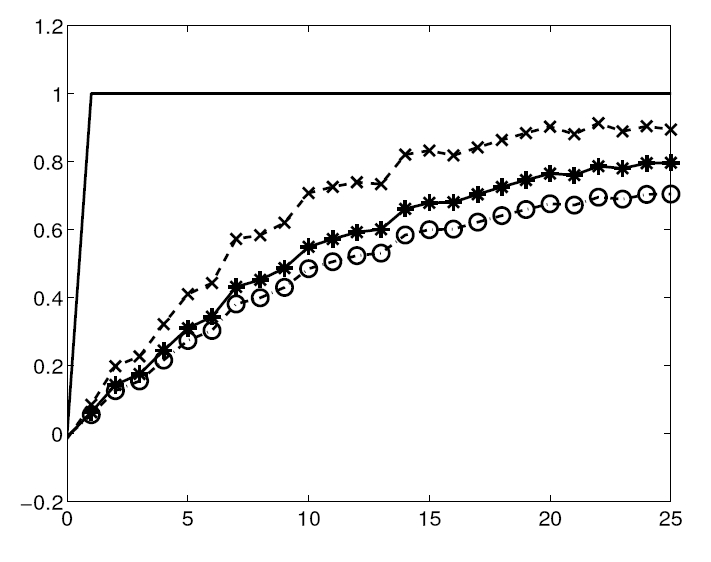
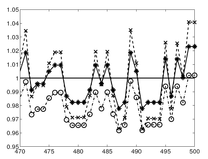
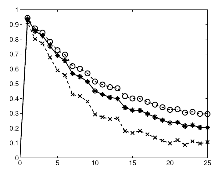
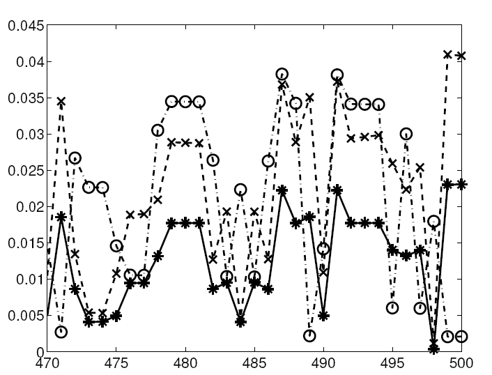
Figure 2: (a) Reconstructed images of 3 methods at close to the image edges. (b) indicates the reconstructed images of 3 methods at the places far away from the image edges. (c) indicates the absolute errors of the three methods at the place close to the image edges. (d) indicates the absolute errors of 3 methods at the places far away from the image edges. The solid line in (a) and (b) are original object function $X_{o}$. The dashed lines with circle mark corresponding to NIRM. The dashed line with cross mark corresponding to TIRM. The solid line with star mark corresponds to LIRM.

In Figure 2 it can be seen that in the place of image edges the TIRM has the smallest error. In the place far away from the edges, The LIRM has lowest errors. Parameter $r$ can be adjusted so the image is optimal at reducing the noise and increasing of the accuracy. The errors of LIRM are less than NIRM in both place of image edges and the place far away from the edges. The errors of TIRM are less than NIRM in the place of image edges but it is at the same level with NIRM at the place far away from the image edges. Normally it is acceptable that there are errors at image edges, but the errors at the place far away from image edges should be as small as possible. Thus LIRM is better than TIRM and NIRM in decrease errors and artifacts.

It can be seen that the results are not dependent on the operator of $T$. It is dependent only with $J$. Here it is assumed that $T$ is Fourier Transform to make things easy. Actually if $J=R\>P=V$ and $V\neq I$ (here $I$ is identical operator), the results of all IRMs (TIRM, LIRM) are not related to the operator $R$ and $P$, but it is dependent to there product $J=V=R\>P$.

For example if a image $G$ is filtered with convolution by operator $F$. Assume the filtered image $G^{\prime}=F\star G$ is known, “$\star$” means convolution. The original image $G$ is required to be recovered from $G^{\prime}$ and the known operator $F$. Assume that the Fourier transform of $F$ is known which is $\tilde{F}=\mathcal{F}\{F$}, $\mathcal{F}$ is Fourier transform. The recover operator $Q=\mathcal{F^{\mathrm{-1}}}(\frac{1}{\tilde{F}})$ can be defined. $\mathcal{F^{\mathrm{-1}}}$ is inverse Fourier transform. $Q$ can fully recover the original image, since if $\tilde{Q}=\mathcal{F}\{Q\}$, $\tilde{Q}\>\tilde{G^{\prime}}=\tilde{Q}\>\tilde{F}\>\tilde{G}=\frac{1}{\tilde{F}}\>\tilde{F}\>\tilde{G}=\tilde{G}$, and hence $Q\star G^{\prime}=G$. However if $\tilde{F}$ has $0$ or very close to $0$ some where. $\tilde{Q}=\frac{1}{\tilde{F}}$ will have “$\frac{1}{0}$”. In this situation, the above image recovery method can not be implemented. Thus a regularization is required. For example $Q=\mathcal{F}(\frac{1}{\tilde{F}+\alpha})$ can be defined, here $\alpha$ small number which is a regularization factor. In this case the recovered image $Q\star G^{\prime}=\mathcal{F}(\frac{\tilde{F}}{\tilde{F}+\alpha})\star G$. $J=Q\star F=\mathcal{F}(\frac{\tilde{F}}{\tilde{F}+\alpha})$. $V=\mathcal{F}(\frac{\tilde{F}}{\tilde{F}+\alpha})$ can be referred as the blurring function. The recovery method can be improved by the IRMs (NIRM, TIRM and LIRM). The results of IRMs are only related to the resolution function $J=V$. If $V$ is same as Eq.(44), the recovered image $G^{\prime}$ will has the same results as the Fig. 1 and 2.

Since to implement the LIRM with the example of CT image reconstruction is very time-consuming, these authors only study the simple examples in this section which is 1-D inverse problem. Note that although in this section, the example of image reconstruction has not been done, the analysis results are still suitable to the situation of CT image reconstruction. In the next section these authors will study another IRM, i.e. SIRM, which is close to LIRM, but is easier to implement for CT image reconstruction.

6 Sub-regional iterative refinement method (SIRM)

6.1 History of SIRM

During the work of iterative reconstruction for LFOV[28, 29], these authors have noticed that not only the truncation artifacts are reduced but the normal artifacts are also reduced. Here the normal artifacts means the artifacts appeared in the reconstruction of FFOV (full field of view) instead of LFOV (limited field of view). Figure 3 shows the normal artifacts appearing with the FBP method, this results is from Matlab.

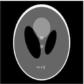
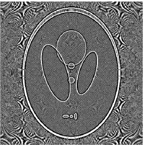
Figure 3: (a) The phantom. (b) The absolute errors of the FBP reconstruction.

If the local inverse reconstruction for LFOV [28, 29] is applied in the situation of FFOV , the algorithm can be summarized as the following,

$$p^{(1)} = p-P\,\Omega\,R\,p$$ (52)

$$X^{r} = R\,p^{(1)}$$ (53)

Where $p=P\,X$. $\Omega$ is the reverse truncation operator, which is defined in the following,

$$\Omega(x)=\left\{\begin{array}[]{cc}0&\textrm{if}\;x\in\textrm{ROI}\\ 1&\textrm{if}\;x\notin\textrm{ROI}\end{array}\right.$$ (54)

Here ROI is the region of interest that is any small arbitrary sub-region where a reconstruction can be made, and $x$ is the coordinates of the pixel of the reconstructed image. In the following example it is assumed that the ROI of the object is a centric disk-shape region and its radius is half of the radius of the image. Here the disk-shape region is chosen because these authors start this kind reconstruction from LFOV which require a disk-shaped region.

Eq.(53) is a simplification of the algorithm[28]. The extrapolation process is take away because this is FFOV instead LFOV. There is no truncation and extrapolation is not necessary. In order to simplify the algorithm Eq.(52,53) further, the truncation operator can be defined as:

$$T(x)=\left\{\begin{array}[]{cc}1&\textrm{if}\;x\in\textrm{ROI}\\ 0&\textrm{if}\;x\notin\textrm{ROI}\end{array}\right.$$ (55)

The relation between the truncation and the reverse truncation operator is given in the following

$$\Omega(x)=1(x)-T(x)$$ (56)

Here $1(x)$ is unit operator with its value as $1$ everywhere on the image. Considering the above Eq.(56), Eq.(52,53) can be rewritten as

$$p^{(1)} = P\,T\,R\,p+(p-P\,R\,p)$$ (57)

$$X^{r} = T\,R\,p^{(1)}$$ (58)

In order further improved the iterative reconstruction, a truncation operator $T$ is added to the reconstructed image of the second formula of Eq.(58). The truncation operator set zeros outside the ROI. This helps to delete unwanted image outside the ROI.

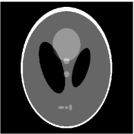
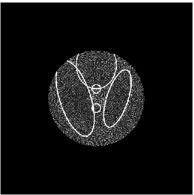
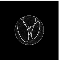
Figure 4: (a) is image of the Shepp-Logan head phantom. (b) is the crop of the image of phantom corresponding to the ROI. (c) is the reconstruction with FBP algorithm. (d) is the reconstruction with the iterative reconstruction algorithm Eq.(57, 58). (e) is the image of the errors for the FBP method or NIRM. (f) is the image of errors for the iterative reconstruction of Eq.(57, 58).

Figure 4 offers the reconstruction results for FBP algorithm and the above iterative algorithm. Figure 4 is the image of the Shepp-Logan head phantom. Figure 4 is the crop of the image of the phantom corresponding to the ROI which is a centered disk. Figure 4 is the reconstruction with FBP algorithm from the simulated parallel beam projections obtained from Matlab. The number of projections is 360 for the half circle scan (180 degree). The space between the two elements of the detector is taken as the same as the space between the two pixels of image. The data size of image of phantom is $512\times 512$. Figure 4 is the reconstruction with iterative algorithm of Eq.(57, 58). The projections and all parameters are same as Figure 4. It is difficult to see the differences between Figure 4 and Figure 4 if you do not see them carefully. An error function is defined as following

$$Err=T\,|X^{r}-X|^{2}$$ (59)

Figure 4 and Figure 4 are error functions corresponding to Figure 4 and Figure 4. Figure 4 and Figure 4 use the same scale of brightness. It is clear that Figure 4 is bright than Figure 4 meaning that the reconstruction errors of FBP algorithm is larger than the iterative algorithm of Eq.(57, 58). It is can be seen that the values of reconstruction with FBP algorithm are little bit lower than the values of the phantom. However the values with iterative reconstruction of Eq.(57, 58) are much close to the values of the phantom. This also shows the improvement of the iterative algorithm Eq.(57, 58).

In the following example the modified Shepp-Logan head phantom is taken in consideration. A massive object is added outside the region of interest. This massive object represents the bone of a human arm. This object can introduce more artifacts for the reconstruction process. The improvement of the iterative reconstruction can be seen more clearly from this example. The stripe artifacts of FBP algorithm are remarkably reduced for this example; see Figure 5.

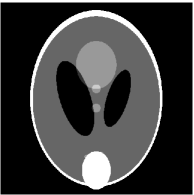
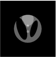
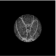
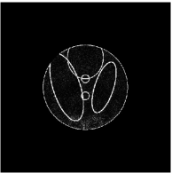
Figure 5: (a) is image of the modified Shepp-Logan head phantom. (b) is crop of the image of phantom corresponding to the ROI. (c) is the reconstruction with FBP algorithm. (d) is the reconstruction with the iterative algorithm of Eq.(58). (e) is the image of the errors for the FBP method or NIRM. (f) is the image of errors for the iterative algorithm of Eq. (58).

6.2 The method

SIRM is sourced from the iterative reconstruction and re-projection algorithm or local inverse method[28], [29] for LFOV. However it requires an improvement to reconstruct the whole image. First, the region of interest (ROI) can be made in any shapes. It is not required that ROI is a round disk-shape region. In the past ROI was chosen as round disk-shape region, this is because of the situation of LFOV. In the following, ROI will be chosen as many small square. The iterative algorithm[28] is used to every square. The extrapolation is taken away because of FFOV. The algorithm was posted on-line in Chinese roughly, see reference [31] and it is summarized more details in the following,

$$p_{i}^{(1)} = p-P\,H_{i}\,X^{(0)}$$ (60)

$$X^{(1)} = \sum_{i=1}^{M}T_{i}\,R\,p_{i}^{(1)}$$ (61)

where $X^{(0)}$ is obtained in Eq.(3); where the subscript $i$ is the index of sub-region which is a small square box; $M$ is the number of sub-regions. $X^{(1)}$ is the iterative reconstruction. Superscript $(1)$ is corresponding to first iteration (the second reconstruction). $p_{i}^{(1)}$ is iterative re-projection for $\omega_{i}$. $\omega_{i}$ is the $i^{th}$ sub-region. After the parts of the object in all sub-regions are reconstructed, all the parts of image are put together to form the reconstructed image $X^{(1)}$. Two truncation operators above are defined in the following

$$H_{i}(x) = \left\{\begin{array}[]{cc}0&\textrm{if}\>x\in\omega_{i}\\ 1&\textrm{if}\>x\notin\omega_{i}\end{array}\right.$$ (64)

$$T_{i}(x) = \left\{\begin{array}[]{cc}1&\textrm{if}\>x\in\omega_{i}\\ 0&\textrm{if}\>x\notin\omega_{i}\end{array}\right.$$ (67)

It is worthwhile to say that the operation $T_{i}(x)$ and $H_{i}(x)$ are normal multiplication. They are different from the operation of $J$ which is corresponding to matrix multiplication. $T_{i}(x)$ is defined $1$ on a sub-region. $H_{i}(x)$ is defined $1$ in the whole region except the sub-region. Hence $H_{i}(x)$ is a hole-shape function. Define unitary operator

$$1(x) \equiv 1$$ (68)

Thus, there is

$$1(x) =H_{i}(x) +T_{i}(x)$$ (69)

Using above equation, Eq.(60) can be written as

$$p_{i}^{(1)} = P\,T_{i}\,X^{(0)}+p-P\,X^{(0)}$$ (70)

However the results of Eq.(60,61) shows cracks between sub-regions. The cracks can be seen in the reconstructed image, see Figure 6. In order to eliminate the cracks, the Eq.(60 or 70) is upgraded as

$$p_{i}^{(1)} = P\,T_{i}^{+}\,X^{(0)}+p-P\,X^{(0)}$$ (71)

where

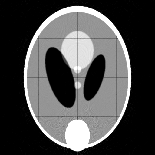
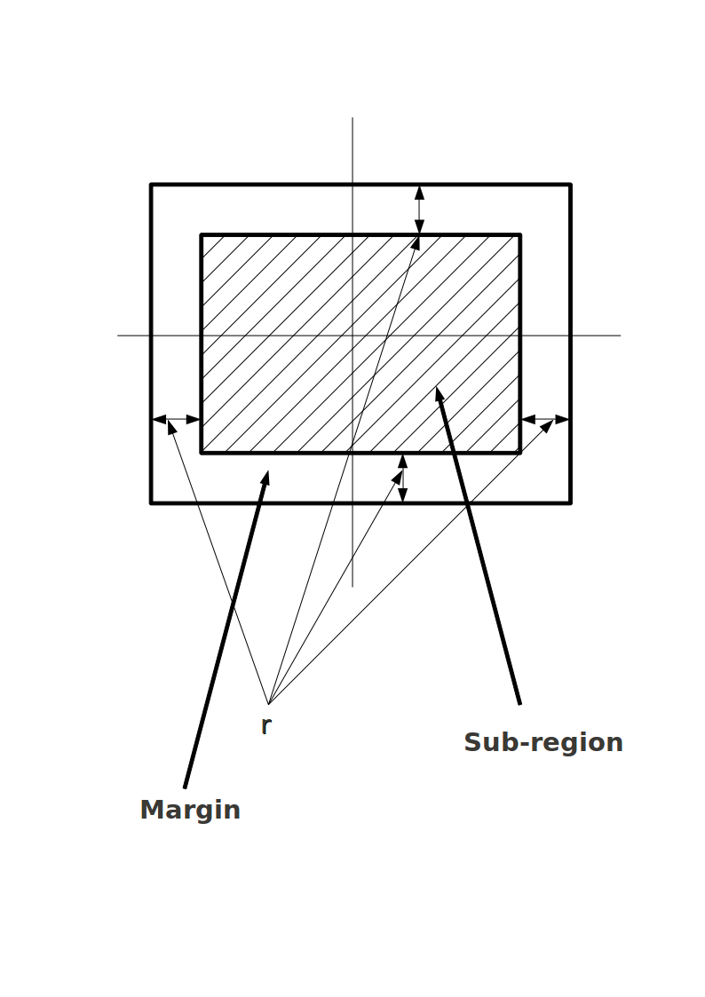
Figure 6: (a) the reconstructed image using Eq.(61). (b) Shows the sub-region and the margin. The margin size is $r$.

$$T_{i}^{+}(x) = \left\{\begin{array}[]{cc}1&\textrm{if}\>x\in\omega_{i}+\mathrm{Margin})\\ 0&\textrm{if}\>x\notin\omega_{i}+\mathrm{Margin})\end{array}\right.$$ (74)

$T_{i}^{+}$ is the image truncation operator with margin, see Figure 6. It was found that if margin size $r$ is taken as $4\sim 10$ pixels, the cracks can be eliminated. But the margin can be chosen as for example 40 if the image size is big. Considering

$$\sum_{i=1}^{M}T_{i}\,f=f$$ (75)

and substituting Eq.(71) to Eq.(61), there is

$$X^{(1)}=(\sum_{i=1}^{M}T_{i}\,R\,P\,T_{i}^{+}X^{(0)})+R\,(p-P\,X^{(0)})$$ (76)

or

$$X^{(1)}=[(\sum_{i=1}^{M}T_{i}\,R\,P\,T_{i}^{+})+(I-J)]X^{(0)}$$ (77)

where $J=R\>P$ defined in Eq.(5). The above formula can be rewritten as,

$$X^{(1)}=F_{SIRM}\,X^{(0)}$$ (78)

$F_{SIRM}$ is a filtering function corresponding to SIRM. The filter function is defined as

$$F_{SIRM}\equiv U+(I-J)$$ (79)

where $U$ is the sub-region projection and reconstruction operator

$$U\equiv\sum_{i=1}^{M}T_{i}\,J\,T_{i}^{+}$$ (80)

Corresponding to Eq.(79), there is,

$$f_{SIRM}(y,x)=u(y,x)+\delta(y,x)-j(y,x)$$ (81)

The above filtering function does not satisfy the unitary condition which keeps the dc value unchanged after the reconstruction compare to the original image. Hence it is required to be upgraded as

$$f_{SIRM}(y,x)=u(y,x)+\eta(x)\,\delta(y,x)-j(y,x)$$ (82)

$\eta(x)$ is normalization function similar to which used in LIRM. Considering the unitary condition

$$\sum_{y}f_{SIRM}(y,x)=1$$ (83)

implies

$$\eta(x)=2-\sum_{y}u(y,x)$$ (84)

Here the summation is taken on the definition area of the variable $y\,\in V$. $V=\sum_{i}\omega_{i}$ is the region of whole image. The Eq.(79) can be replaced as

$$F_{SIRM}\equiv\eta I-J+U$$ (85)

Usually $\eta(x)$ can be taken as

$$\eta(x)\approx 1$$ (86)

Only if the sub-region ($\omega_{i}$) is very small, $\eta(x)$ is possible to be significantly different from $1$. This is same as the case of the LIRM discussed in last section. The resolution function of SIRM algorithm is $F_{SIRM}\>J$.

The biggest difference of the form of SIRM from TIRM is the operator $U$ in Eq.(80) comparing Eq.(85) and Eq.(17). In order to have a good understanding of this operator, the process of this operator is shown in Fig. 7. Fig. 7 illustrates the first reconstruction $X^{(0)}=R\,p$. Fig. 7 shows that the image of Fig. 7 is divided into sub-regions $T_{i}^{+}\,X^{(0)}\;i=1,2,....M$. Fig. 7 shows that the sub-region images of (b) are reprojected $P\,T_{i}^{+}\,X^{(0)}\;i=1,2,....M$. Fig. 7 shows that the sub-region image is reconstructed from Fig. 7 by using $R\,P\,T_{i}\,X^{(0)}\;i=1,2,....M$. Fig. 7 shows that the sub-region images are put together to form a whole image by using $U\,X^{(0)}=\sum_{i=1}^{M}T_{i}\,R\,P\,T_{i}^{+}X^{(0)}$.

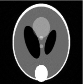
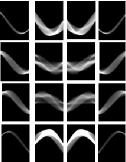
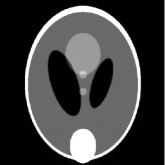
Figure 7: $U\,X^{(0)}=\sum_{i=1}^{M}T_{i}\,R\,P\,T_{i}^{+}X^{(0)}$. (a) The first reconstruction. (b) The image of (a) is divided in sub-regions. (c)The sub-region images of (b) are reprojected. (d) The sub-region images are reconstructed from (c). (e) The sub-region images are put together to form a whole image: $U\,X^{(0)}$.

The original image Fig. 7 is chosen as the modified Shepp-Logan head phantom with data size $512\times 512$. The modification is adding a massive small disk to the bottom of the image. The massive small disk will increase the normal artifacts, which will be utilized to test the algorithms in the next paragraph. The projection operator $P$ is parallel beam and defined in Matlab. The projections data is created by the operator $P$ to the above modified Shepp-Logan head phantom. The number of projections is 360 for the half circle scan (180 degree); the space between the two elements of the detector is taken equal to the space between the two pixels of image. The operator $R$ is corresponding to NIRM which is filtered back projection method which is defined in Matlab.

The process of operator $U$ shown in Fig. 7 looks mediocre. Actually, it is really not mediocre because the margins in the algorithm plays an important role in eliminating artifacts and decreasing the noises.

In the limit case $\omega_{i}$ is small as only one pixel,

$$\sum_{i=1}^{M}T_{i}=1(x)$$ (87)

$$J\,T_{i}^{+}=K$$ (88)

Here $K$ is defined in Eq.(21), Hence considering Eq.(80), there is

$$U=K$$ (89)

Considering Eq.(85) Eq.(33) there is SIRM$\rightarrow$LIRM in the case $\omega_{i}\rightarrow$one pixel.

6.3 The iterative algorithm with more loops

In the above discussion, two algorithms are iterated with only one loop. If one loop does not satisfy, more loops can be utilized, this can be written as

$$X_{l}^{(n)}=F_{l}^{n}\,X^{(0)}$$ (90)

where $X_{l}^{(n)}$ is the reconstructed image with more loops of iteration. $n$ is the iteration number. $F_{l}^{n}=(F_{l})^{n}$ is the filtering operator for iteration number $n$. $l$ indicates different algorithm, $l=\{TIRM,\,LIRM,\,SIRM\}$. The resolution function with more loops is

$$J_{l}^{(n)}=F_{l}^{n}J$$ (91)

For the reconstructions, the error is defined as

$$Err_{l}^{(n)}\equiv X_{l}^{(n)}-X_{o}$$ (92)

$X_{l}^{(n)}$ is defined in Eq.(90). $X_{o}$ is the object or the original image. Considering Eq.(3) and Eq.(90) the error can be defined as

$$Err_{l}^{(n)}=(F_{l}^{n}J-I)X_{o}+F_{l}^{n}\,R\,p_{n}$$ (93)

The first item of the above formula is corresponding to artifacts which is related to the original image $X_{o}$; the second item is corresponding to noises which is related to noises in the first reconstruction $R\,p_{n}$. The error for NIRM method is $Err^{(0)}=(J-I)X_{o}-R\>p_{n}$. The artifact transfer function can be defined as

$$A_{l}^{n}=F_{l}^{n}J-I$$ (94)

and the noise transfer function can be defined as

$$N_{l}^{n}=F_{l}^{n}\>R$$ (95)

The noise transfer function and the artifact transfer function have different forms, which gives the possibility to optimize the algorithm by balancing the artifacts and the noises and adjusting the filtering function.

The absolute error $|Err_{l}^{(n)}|$ will be used to study reconstruction results. The distance between the reconstructed image $X_{l}^{(n)}$ and the original image $X$ can be used also to compare the reconstruction. The distance is defined in the following,

$$d_{l}^{(n)}=\frac{\sum_{x}(X_{l}^{(n)}(x)-X_{o}(x))^{2}}{\sum_{x}(X(x)-\bar{X}_{o}(x))^{2}}$$ (96)

where $\bar{X}$ is the average of the image $X(x)$. See reference[15] for details of the definition of the distance.

6.4 Results

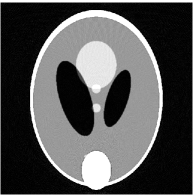
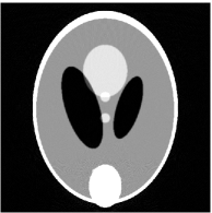
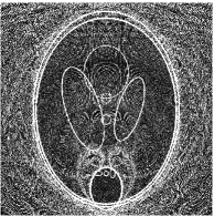
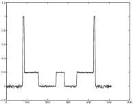
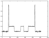
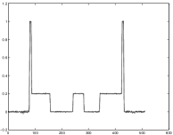
Figure 8: The reconstructions of different algorithms. (a) The reconstruction with NIRM. (b) The reconstruction with TIRM . (c) The reconstruction with SIRM. (d), (e) and (f) are the absolute errors corresponding to image (a), (b) and (c) respectively. (g), (h) and (i) are the profiles along x-axis corresponding to image (a), (b) and (c).

Figure 8 shows the comparison of SIRM with NIRM and TIRM. NIRM is implemented in Eq(). TIRM is implemented with Eq.(15). $\eta$ in Eq.(82) is chosen as $1$ for simplification. SIRM is implemented with Eq.(77). The region of the object is divided according to $4\,\times\,4$ grid for SIRM. Hence, there are $M=16$ sub-regions. The margin is chosen as $10$ pixels. The iteration for Eq.(90) are done with only one loop, i.e. $n=1$ .

The original image $X_{o}$, the projection projector $P$ and the reconstruction operator $R$ are chosen the same as in Fig. 7, see section 5.2. The projections $p$ is obtained through the simulation with $p=P\,X$. In this example additional noises $p_{n}$ are not added to the projections. However, since there are always calculation errors, $p_{n}\neq 0$ in general.

SIRM yielded the best reconstruction results than the NIRM and the TIRM. The stripe artifacts shown on Figure 8 are reduced remarkably on Figure 8. The absolute errors $|Err^{(0)}|$ shown in Figure 8 $|Err_{l=NRRM}^{(0)}|$ and Figure 8 $|Err_{l=TRRM}^{(1)}|$ are larger than in Figure 8 $|Err_{l=SRRM}^{(1)}|$. The results of TIRM (Figure 8,8) are similar to the results of NIRM method (Figure 8,8).

It is important to mention that: A) in Figure 8 the absolute errors on the two sub-regions containing the massive disk are little bit larger than the errors in other sub-regions. This drawback can be eliminated through increasing the number of sub-regions, for example using $16\times 16$ grid instead of $4\times 4$ grid. In practice, the smaller sub-regions are required to be used only in the two sub-regions containing the massive disk. B) the above results of the iterative algorithm are only done with one loop of iteration and further more loops using Eq.(90) can also improve the results, but the improvement is limited. C) If LIRM is implemented, since the sub-region becomes as small as only one pixel(voxel), the result should be better (in the meaning of reducing the artifacts and decreasing the noises) than SIRM if the same margin $r$ is used. LIRM is more time-consuming, to implement it more modern technologies for example GPU parallel calculation and fast back-projection techniques are required. The implementation of LIRM will be left for the future work.

Methods:	Distance:
NIRM Eq.(3)	0.0177
TIRM Eq.(15)	0.0134
SIRM Eq.(77)	0.0172

Table 1: The distance for different methods

The distances for the above three algorithms have been calculated. Table 1 tells that the distance from the reconstruction of SIRM to the phantom is smaller than the distance from the reconstruction of NIRM to the phantom. However, the smallest distance is obtained through TIRM. Do these results mean that the reconstruction results from the TIRM is better than SIRM? The following details of the profiles give the answer.

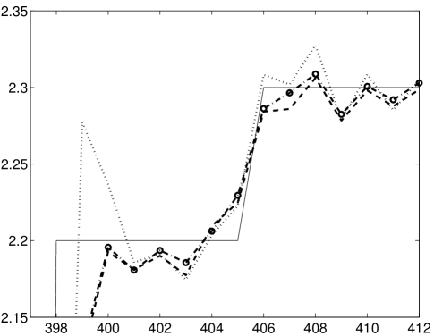
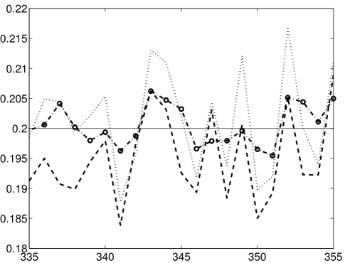
Figure 9: The central profiles along the vertical direction of Figure 8, 8, 8. (a) is the zoomed image at the place close to the edge of different image structures. (b) is the zoomed image at the place far away from the edge of different image structures. In the two figures, the solid line corresponds to the phantom; the dashed line is corresponding to NIRM; the dotted line corresponds to TIRM; the dash-dot line with circle marks corresponds to SIRM.

Table 1 tells that the TIRM has the smallest distance. However, TIRM has an over correction at the image edges. The over correction can be seen in Fig. 9. Here the dotted line is far away from the solid line compared to dashed line and dash-dot line. The dashed line and dash-dot line are close to each other. Fig. 9 shows that TIRM has a over correction at the image edges. The areas close to the edge of the different image structures are strongly relayed to the distance defined in Eq.(96). This kind of over correction can reduce the distance, but it causes the reconstructed image to be oscillated at the image edges. In a clinical cases the over correction can not be accepted. The over correction is easy to be thought as some kind of real structure, it is dangerous to clinical situation. Even though TIRM has the smallest distance, the reconstructed image through TIRM is noisier than other two algorithms. TIRM is rarely used directly in clinics. The reference [10] is the example of indirectly using TIRM. It is TIRM plus pre-filtering and post-filtering in the reconstruction. Pre-filtering can cause the lose of information.

In contrast, the SIRM reduces the oscillation at the place close to the edges and reduces the artifacts at the place far away from the edges simultaneously, which can be seen in Figure 9. Here the dash-dot line is the closest line to the solid line. The dash-dot line is corresponding to SIRM.

According to the above discussion, SIRM and LIRM have better quality compared with NIRM and TIRM in image reconstruction with FFOV.

7 Conclusions and future work

Two generalized iterative refinement methods LIRM and SIRM have been introduced. As an example, simple inverse problem to utilize LIRM has been given. The LIRM eliminates the over correction and it is less noise sensitive comparing to TIRM.

SIRM has been applied to the CT image reconstruction from untruncated parallel-beam projections. The simulations shown that it can reduce the normal artifacts remarkably, which exists in the reconstruction with FBP algorithm. SIRM has been compared to the TIRM and NIRM. The result shows that the SIRM has less artifacts in reconstructed image and TIRM is more sensitive to noises. The distance of SIRM is smaller than NIRM. The smallest distance is obtained through TIRM. However the smallest distance is achieved through an over-correction in the places close to the image edges, which can not be accepted.

These authors have shown that LIRM is a special case of SIRM. NIRM and TIRM are special cases of LIRM. Hence LIRM and SIRM are two generalized iterative refinement reconstruction methods. SIRM and LIRM can be seen as local inverse applied to the image reconstruction of full field of veiw. Hence, SIRM and LIRM can be seen as generalized iterative refinement method(GIRM) and local inverse method for FFOV. SIRM and LIRM do not minimize the noise or artifacts alone but minimize the total values of the noise and artifacts. Even the SIRM and LIRM are developed in the field of CT image reconstruction, these authors believe they are a general methods and can be applied widely in physics and applied mathematics where IRM can be applied.

The future work of these authors is to implement the LIRM in CT image reconstruction. these authors also plan to implement SIRM and LIRM in fan-beam and cone-beam geometries.

References

- [1] http://en.wikipedia.org/wiki/Iterative_refinement
- [2] Kak A C and Slaney M 1988 Principles of Computerized Tomographic Imaging IEEE Press
- [3] L. Chang. A method for attenuation correction in radionuclide computed tomography. IEEE Transactions on Nuclear Science, 25(1):638–642, 1978.
- [4] K. Zeng, Z. Chen, L. Zhang, and G. Wang. An error-reduction-based algo- rithm for cone-beam computed tomography. Medical Physics, 31(12):3206– 3212, 2004.
- [5] C Riddell, B Bendriem, M H Bourguignon, and J P Kernevez. The ap- proximate inverse and conjugate gradient: non-symmetrical algorithms for fast attenuation correction in SPECT. Physics in Medicine and Biology, 40(2):269, 1995.
- [6] J. D. O’Sullivan. A fast sinc function gridding algorithm for fourier inversion in computer tomography. IEEE Transactions on Medical Imaging, 4(4):200– 207, 1985.
- [7] A. H. Delaney and Y. Bresler. A fast and accurate Fourier algorithm for it- erative parallel-beam tomography. IEEE Transactions on Image Processing, 5(5):740–753, 1996.
- [8] Noo F, Defrise M, Clackdoyle R, and Kudo H, “Image reconstruction from fan-beam projections on less than a short scan”, Phys. Med. Biol., vol. 47, pp. 2525-2546, 2002.
- [9] Parker, DL, “Optimal short scan convolution reconstruction for fan beam CT”, Med. Phys., vol. 9, pp. 254-257, 1982.
- [10] Johan Sunnegardh, Iterative Filtered Backprojection Methods for Helical Cone-Beam CT, Link¨ping Studies in Science and Technology o Dissertation No. 1264. August 2009
- [11] Zhao S R, Halling H 1993 Image reconstruction for Fan beam X-ray Tomography Using a new Integral Transform pair VI International Symposium on Computerized Tomography, Novosibirsk, Russia, Abstracts ed. M.M. Lavrentev 125
- [12] Nilsson M 2003 Local Tomography at glance Thesis, Mathematics, Centre for Mathematical Sciences, Lund University, ISSN 1404-028X, ISBN 91-628-5741-X, LUTFMA-2007
- [13] Seger M M 2002 Ramp filter implementation on truncated projection data, application to 3D linear tomography for logs Proceedings SSAB Symposium on Image Analysis, Lund, Sweden Editor Astrom
- [14] Nassi M, Brody W R, Medoff B P, Macovski A 1982 Iterative reconstruction-reprojection: an algorithm for limited data cardiac-computed tomography IEEE trans. Biomed. Engineering 295 333-340
- [15] Cho P S, Rudd A D and Johnson R H 1996 Cone-beam CT from width truncated projections Computerized Medical Imaging and Graphics 20 49-57
- [16] Faridani A, Ritman E L and Smith K T 1992 Local tomography SIAM. J. APPL. MATH. 52 459-84
- [17] Rashid-Farrokhi F, Liu K J R, Berenstein C A and Walnut D 1997 Wavelet-based multiresolution local tomography IEEE Transactions on Image Processing 6 1412-30
- [18] Feldkamp L A, Davis L C and Kress J W 1984 Practical cone-beam algorithm J. Opt. Soc. Am. 1 612-19
- [19] Smith B D 1985 Image Reconstruction from cone-beam projections: necessary and sufficient conditions IEEE transactions on Medical Image 4 14-25
- [20] Grangeat P, Mathematical framework of cone beam 3D reconstruction via the first derivative of the Radon transform G. T. Herman, A.K. Louis, and F. Natterer (eds.) Mathematical methods in tomography, Lecture notes in mathematics No. 1497, Springer Verlag 66-97
- [21] Defrise M and Clack R 1994 A cone-beam Reconstruction algorithm using shift Variant Filtering and cone-beam backprojection IEEE trans. on Medical Imaging 13 186-195
- [22] 6. Zhao, S.-R. Halling, H. A new Fourier method for fan beam reconstruction. Source: 1995 IEEE Nuclear Science Symposium and Medical Imaging Conference Record (Cat. No.95CH35898), p 1287-91 vol.2, 1995
- [23] Shuangren Zhao, Kang Yang, Kevin Yang, Fan beam Image Reconstruction with Generalized Fourier Slice Theorem, accepted by Journal of X-Ray Science and Technology 2014
- [24] Zhao S R and Halling H 1995 Reconstruction of cone beam projection with free source path by a generalized Fourier method Proceedings of the international meeting on fully three-dimensional image reconstruction in radiology and nuclear medicine 323
- [25] Katsevich A 1999 Cone beam Local Tomography SIAM J. APPL. MATH. 59 2224-2246
- [26] Katsevich A 2002 Theoretically exact Filtered backprojection-type Inversion algorithm for spiral CT SIAM J. App. MATH. 62 2012-2026
- [27] Kim J H, KWAK K Y, Park S B, and Cho Z H 1985 Projection Space Iteration Reconstruction-Reprojection IEEE transaction on Medical Imageing 4 139
- [28] Zhao S R and Jaffray D A 2004 Iterative reconstruction-reprojection for truncated projections Med. Phys. 31 1719
- [29] Shuangren Zhao, Kang Yang , Dazong Jiang and Xintie Yang, Interior reconstruction using local inverse, Journal of X-Ray Science and Technology, 2011 Jan 1;19 (3):403-15
- [30] Shuangren Zhao, Kang Yang and Xintie Yang, Reconstruction from truncated projections using mixed extrapolations of exponential and quadratic functions, Journal of X-Ray Science and Technology, Volume 19, Number 2 / 2011 P 155-172
- [31] Shuangren Zhao, XinTie Yang, Iterative reconstruction in all sub-regions, Sciencepaper online Vol 1 No. 4, Nov. 2006 P301-308
- [32] W. Moench, Freiberg, Algorithm / Algorithmus 46 Iterative Refinement of Approximations to a Generalized Inverse of a Matrix. Computing 28, 79–87 (1982)
- [33] Xuan Fei, Zhihui Wei, and Liang Xiao, Iterative refinement of computing inverse matrix,International Journal of Computer Mathematics Vol. 86, No. 7, July 2009, 1126–1134
- [34] LIN HE, TI-CHIUN CHANG, STANLEY OSHER, TONG FANG, AND PETER SPEIER, MR IMAGE RECONSTRUCTION BY USING THE ITERATIVE REFINEMENT METHOD AND NONLINEAR INVERSE SCALE SPACE METHODS, UCLA CAM Report, 2006
- [35] Anders M. N. Niklasson, Iterative refinement method for the approximate factorization of a matrix inverse PHYSICAL REVIEW B 70, 193102 (2004).
- [36] Haricharan Lakshman, Martin K¨oppel, Patrick Ndjiki-Nya and Thomas Wiegand, IMAGE RECOVERY USING SPARSE RECONSTRUCTION BASED TEXTURE REFINEMENT, Acoustics Speech and Signal Processing (ICASSP), 2010 IEEE International Conference on Date of Conference: 14-19 March 2010
- [37] Shin’ichi Oishi, Iterative Refinement for Ill-conditioned Linear Equations, 2008 International Symposium on Nonlinear Theory and its Applications NOLTA’08, Budapest, Hungary, September 7-10, 2008
- [38] Wei-Pai Tangy, Refining an Approximate Inverse, Appeared in J. of Comp. and Appl. Math, 2000, vol. 123 (Numerical Analysis 2000 vol. III: Linear Algebra), pp. 293–306.
- [39]
- [40] Frédéric Noo et al (2002). Image reconstruction from fan-beam projections on less than a short scan, Physics in Medicine and Biology, Volume 47 Number 14, Page 311 doi:10.1088/0031-9155/47/14/311
- [41] Yu Zou, Xiaochuan Pan and Emil Y Sidky (2005). Image reconstruction in regions-of-interest from truncated projections in a reduced fan-beam scan Physics in Medicine and Biology Volume 50 Number 1 page 002 doi:10.1088/0031-9155/50/1/002
- [42] Kudo, H. ; Univ. of Tsukuba, Japan ; Noo, F. ; Defrise, M. ; Clackdoyle, R. (2002). New super-short-scan algorithms for fan-beam and cone-beam reconstruction Nuclear Science Symposium Conference Record, 2002 IEEE (Volume:2 ) Date of Conference: 10-16 Nov. 2002
- [43] Yu Zou and Xiaochuan Pan (2004). Exact image reconstruction on PI-lines from minimum data in helical cone-beam CT Phys Med Biol. 2004 Mar 21;49(6):941-59.
- [44] Zhang-O’Connor, Y.; Fessler, J.A. (2006). "Fourier-Based Forward and Back-Projectors in Iterative Fan-Beam Tomographic Image Reconstruction." IEEE Transactions on Medical Imaging 25(5): 582-589. <http://hdl.handle.net/2027.42/86013>
- [45] Robert Cierniak (2009). New neural network algorithm for image reconstruction from fan-beam projections Neurocomputing Volume 72, Issues 13–15, August 2009, Pages 3238–3244
- [46] Xiangyang Tang, Jiang Hsieh, Roy A Nilsen, Sandeep Dutta, Dmitry Samsonov and Akira Hagiwara (2006). A three-dimensional-weighted cone beam filtered backprojection (CB-FBP) algorithm for image reconstruction in volumetric CT—helical scanning Physics in Medicine and Biology Volume 51 Number 4 page 007
- [47] Stefan Schaller ; Karl Stierstorfer ; Herbert Bruder ; Marc Kachelriess ; Thomas Flohr (2001) Novel approximate approach for high-quality image reconstruction in helical cone-beam CT at arbitrary pitch Proc. SPIE 4322, Medical Imaging 2001: Image Processing, 113 (July 3, 2001);
- [48] Bonnet, S. ; CREATIS, CNRS, Villeurbanne, France ; Peyrin, F. ; Turjman, F. ; Prost, R. (2002) Multiresolution reconstruction in fan-beam tomography Image Processing, IEEE Transactions on (Volume:11 , Issue: 3 ) Mar 2002, Page(s):169 - 176
- [49] Jeffrey H. Siewerdsen and David A. Jaffray (2001) Cone-beam computed tomography with a flat-panel imager: Magnitude and effects of x-ray scatter Med. Phys. 28, 220 (2001); Page 169 - 176
- [50] Zigang Wang, Guoping Han ; Tianfang Li ; Zhengrong Liang (2005). Speedup OS-EM image reconstruction by PC graphics card technologies for quantitative SPECT with varying focal-length fan-beam collimation Nuclear Science, IEEE Transactions on (Volume:52 , Issue: 5 ) Oct. 2005, Page(s): 1274 - 1280
- [51] Jing Wang, Hongbing Lu, Tianfang Li and Zhengrong Liang (2005) An alternative solution to the nonuniform noise propagation problem in fan-beam FBP image reconstruction Med. Phys. 32, 3389 (2005); http://dx.doi.org/10.1118/1.2064807
- [52] Yu, D.F. ; Michigan Univ., Ann Arbor, MI, USA ; Fessler, J.A. ; Ficaro, E.P. (2000). Maximum-likelihood transmission image reconstruction for overlapping transmission beams Medical Imaging, IEEE Transactions on (Volume:19 , Issue: 11 ), Nov. 2000, Page(s):1094 - 1105
- [53] Sidky Chien-Min Kao Xiaochuan Pan (2006). Effect of the data constraint on few-view, fan-beam CT image reconstruction by TV minimization 2006 IEEE Nuclear Science Symposium Conference Record, 2006 | 4 | 2296 - 2298
- [54] Jiang Hsieh, Robert C. Molthen, Christopher A. Dawson and Roger H. Johnson (2000). An iterative approach to the beam hardening correction in cone beam CT Med. Phys. 27, 23 (2000); http://dx.doi.org/10.1118/1.598853
- [55] Elbakri, I.A. ; Dept. of Electr. Eng. & Comput. Sci., Michigan Univ., Ann Arbor, MI, USA ; Fessler, J.A. (2002). Statistical image reconstruction for polyenergetic X-ray computed tomography Medical Imaging, IEEE Transactions on (Volume:21 , Issue: 2 ) Feb. 2002 Page(s):89 - 99
- [56] Ying Liu, Hong Liu, Ying Wang and Ge Wang Half-scan cone-beam CT fluoroscopy with multiple x-ray sources Med. Phys. 28, 1466 (2001); http://dx.doi.org/10.1118/1.1381549
- [57] Shuai Leng, Tingliang Zhuang, Brian E Nett and Guang-Hong Chen (2005). Exact fan-beam image reconstruction algorithm for truncated projection data acquired from an asymmetric half-size detector 2005 Phys. Med. Biol. 50 1805 doi:10.1088/0031-9155/50/8/012
- [58] Adam Wunderlich and Frédéric Noo (2008) Image covariance and lesion detectability in direct fan-beam x-ray computed tomography 2008 Physics in Medicine and Biology Volume 53 Number 10 Page: 2471 doi:10.1088/0031-9155/53/10/002
- [59] Thomas G. Flohr, Shuai Leng, Lifeng Yu, Thomas Allmendinger, Herbert Bruder, Martin Petersilka, Christian D. Eusemann, Karl Stierstorfer, Bernhard Schmidt and Cynthia H. McCollough (2009). Dual-source spiral CT with pitch up to 3.2 and 75 ms temporal resolution: Image reconstruction and assessment of image quality Med. Phys. 36, 5641 (2009); http://dx.doi.org/10.1118/1.3259739
- [60] Yangbo Ye, Hengyong Yu, Yuchuan Wei and Ge Wang (2007). A general local reconstruction approach based on a truncated Hilbert transform Journal of Biomedical Imaging archive, Volume 2007 Issue 1, January 2007 Pages 2-2
- [61] Xiaochuan Pan, Emil Y Sidky, and Michael Vannier (2009). Why do commercial CT scanners still employ traditional, filtered back-projection for image reconstruction? Inverse Problems 25 123009 doi:10.1088/0266-5611/25/12/123009
- [62] Zeng L, Liu B, Liu L, Xiang C. (2010). A new iterative reconstruction algorithm for 2D exterior fan-beam CT J Xray Sci Technol. 2010;18(3):267-77. doi: 10.3233/XST-2010-0259.
- [63] Xun Jia, Yifei Lou, Ruijiang Li, William Y. Song and Steve B. Jiang (2010). GPU-based fast cone beam CT reconstruction from undersampled and noisy projection data via total variation Med. Phys. 37, 1757 (2010); http://dx.doi.org/10.1118/1.3371691
- [64] Kihwan Choi, Jing Wang, Lei Zhu, Tae-Suk Suh, Stephen Boyd and Lei Xing (2010) Compressed sensing based cone-beam computed tomography reconstruction with a first-order method Med. Phys. 37, 5113 (2010); http://dx.doi.org/10.1118/1.3481510
- [65] Hengyong Yu and Ge Wang (2009). Compressed sensing based interior tomography Phys. Med. Biol. 54 2791 doi:10.1088/0031-9155/54/9/014
- [66] Li L, Kang K, Chen Z, Zhang L, Xing Y. A general region-of-interest image reconstruction approach with truncated Hilbert transform J Xray Sci Technol. 2009;17(2):135-52. doi: 10.3233/XST-2009-0218.
- [67] Averbuch, A. ; Sch. of Comput. Sci., Tel Aviv Univ., Tel Aviv, Israel ; Sedelnikov, I. ; Shkolnisky, Y. (2012). CT Reconstruction From Parallel and Fan-Beam Projections by a 2-D Discrete Radon Transform Image Processing, IEEE Transactions on (Volume:21 , Issue: 2 ) Feb. 2012 Page(s):733 - 741
- [68] A. V. Narasimhadhan, Aman Sharma, Dipen Mistry (2013). Image Reconstruction from Fan-Beam Projections without Back-Projection Weight in a 2-D Dynamic CT: Compensation of Time-Dependent Rotational, Uniform Scaling and Translational Deformations Open Journal of Medical Imaging, 2013, 3, 136-143 Published Online December 2013 (http://www.scirp.org/journal/ojmi) http://dx.doi.org/10.4236/ojmi.2013.34021
- [69] Wang G, Wei Y On a derivative-free fan-beam reconstruction formula IEEE Trans Image Process. 1993;2(4):543-7.
- [70] J Fu, P Li, Q L Wang, S Y Wang, M Bech, A Tapfer, D Hahn and F Pfeiffer (2011). A reconstruction method for equidistant fan beam differential phase contrast computed tomography Phys. Med. Biol. 56 4529 doi:10.1088/0031-9155/56/14/019
- [71] Jiang Hsieh, Brian Nett, Zhou Yu, Ken Sauer,Jean-Baptiste Thibault, Charles A. Bouman Recent Advances in CT Image Reconstruction Current Radiology Reports (2013) 1:39–51
- [72] Altaf H. Khana, Reaz A. Chaudhurib, Fan-beam geometry based inversion algorithm in computed tomography (CT) for imaging of composite materials, Composite Structures Volume 110, April 2014, Pages 297–304,DOI 10.1007/s40134-012-0003-7
- [73] Schomberg, H. ; Philips Res. Lab., Hamburg, Germany ; Timmer, J. The gridding method for image reconstruction by Fourier transformation (1995) Medical Imaging, IEEE Transactions on (Volume:14 , Issue: 3 ) Sep 1995 Page(s):596 - 607
- [74] Wang, G. ; Mallinckrodt Inst. of Radiol., Washington Univ., St. Louis, MO, USA ; Lin, T.-H. ; Cheng, Ping-Chin ; Shinozaki, D.M. (1993). A general cone-beam reconstruction algorithm Medical Imaging, IEEE Transactions on (Volume:12 , Issue: 3 ) Sep 1993 Page(s): 486 - 496
- [75] Stefan Schaller ; Thomas Flohr ; Peter Steffen New efficient Fourier-reconstruction method for approximate image reconstruction in spiral cone-beam CT at small cone angles Proc. SPIE 3032, Medical Imaging 1997: Physics of Medical Imaging, 213 (May 2, 1997); doi:10.1117/12.273987
- [76] Ryan Hass and Adel Faridani, Regions of Backprojection and Comet Tail Artifacts for $\pi$-Line Reconstruction Formulas in Tomography, SIAM J. Imaging Sci. 5-4 (2012), pp. 1159-1184 http://dx.doi.org/10.1137/110857623
- [77] Chuang Miao, Baodong Liu, Qiong Xu, Hengyong Yu, An improved distance-driven method for projection and backprojection, Journal of X-Ray Science and Technology, Volume 22, Number 1 / 2014 Pages 1-18 DOI 10.3233/XST-130405
- [78] Xianchao Wang, Ziyue Tang, Bin Yan, Lei Li, Shanglian Bao, Interior reconstruction method based on rotation-translation scanning model, Journal of X-Ray Science and Technology, Volume 22, Number 1 / 2014 Pages 37-45 DOI 10.3233/XST-130407
- [79] Xiaobing Zou, Hengyong Yu, Li Zeng, Laplace operator based reconstruction algorithm for truncated spiral cone beam computed tomography Journal of X-Ray Science and Technology, Volume 21, Number 4 / 2013, Pages:515-526,DOI:10.3233/XST-130398
- [80] Shaojie Tang, Yi Yang, Xiangyang Tang Practical interior tomography with radial Hilbert filtering and a priori knowledge in a small round area Journal of X-Ray Science and Technology,Volume 20, Number 4 / 2012,Pages 405-422,DOI 10.3233/XST-2012-00348
- [81] Pascal Thériault Lauzier, Jie Tang and Guang-Hong Chen Time-resolved cardiac interventional cone-beam CT reconstruction from fully truncated projections using the prior image constrained compressed sensing (PICCS) algorithm FEATURED ARTICLE 2012 Phys. Med. Biol. 57 2461 doi:10.1088/0031-9155/57/9/2461
- [82] Alexander Kostenko, K. Joost Batenburg, Andrew King, S. Erik Offerman, and Lucas J. van Vliet, Total variation minimization approach in in-line x-ray phase-contrast tomography, Optics Express, Vol. 21, Issue 10, pp. 12185-12196 (2013) http://dx.doi.org/10.1364/OE.21.012185
- [83] J. Hsieh, E. Chao, J. Thibault, B. Grekowicz, A. Horst, S. McOlash and T.J. Myers, A novel reconstruction algorithm to extend the CT scan fieldofview, Medical Phys 31 (2004), 2385–2391.
- [84] M. Nassi,W.R. Brody, B.P.Medoff and A.Macovski, Iterative reconstructionreprojection: an algorithm for limited data cardiaccomputed tomography, IEEE trans Biomed Engineering 295 (1982), 333–340.
- [85] J.H. Kim, K.Y. KWAK, S.B. Park and Z.H. Cho, Projection space iteration reconstruction reprojection, IEEE transaction on Medical Imaging 4 (1983), 139–143B.
- [86] Ohnesorge, T. Flohr, K. Schwarz, J.P. Heiken and K.T. Bae, 2000 Efficient correction for CT image artifacts caused by objects extending outside the scan field of view, Med Phys 27, 39–46.
- [87] M.M. Seger, Rampfilter implementation on truncated projection data. Application to 3D linear tomography for logs,Proceedings SSAB02, Symposium on Image Analysis, Lund, Sweden, 7–8 March 2002. Editor Astrom.
- [88] Rashid-Farrokhi, K.J.R. Liu, C.A. Berenstein and D.Walnut,Wavelet-based Multiresolution Local Tomography, IEEE Transactions on Image Processing 6 (1997), 1412–1430.