Variational tensor network renormalization in imaginary time:
Two-dimensional quantum compass model at finite temperature

Abstract

Progress in describing thermodynamic phase transitions in quantum systems is obtained by noticing that the Gibbs operator $e^{-\beta H}$ for a two-dimensional (2D) lattice system with a Hamiltonian $H$ can be represented by a three-dimensional tensor network, the third dimension being the imaginary time (inverse temperature) $\beta$. Coarse-graining the network along $\beta$ results in a 2D projected entangled-pair operator (PEPO) with a finite bond dimension $D$. The coarse-graining is performed by a tree tensor network of isometries. The isometries are optimized variationally — taking into account full tensor environment — to maximize the accuracy of the PEPO. The algorithm is applied to the isotropic quantum compass model on an infinite square lattice near a symmetry-breaking phase transition at finite temperature. From the linear susceptibility in the symmetric phase and the order parameter in the symmetry-broken phase the critical temperature is estimated at ${\cal T}_{c}=0.0606(4)J$, where $J$ is the isotropic coupling constant between $S=1/2$ pseudospins.

I Introduction

Understanding phase transitions and broken symmetries in frustrated many-body quantum systems remains one of the major challenges of modern physics. Frustration in magnetic systems occurs by competing exchange interactions and leads frequently to disordered spin liquids Nor09 ; Bal10 . However, this does not happen in two-dimensional (2D) classical systems where ordered states with broken $\mathbb{Z}_{2}$ symmetry occur at finite temperature, as in the exactly solvable Ising models with fully frustrated lattice, or with frustration distributed periodically along columns Vil77 ; Lon80 . In contrast, quantum spins interacting by SU(2) symmetric interactions order only at zero temperature in the 2D Heisenberg model. Whether or not 2D quantum spin models with interactions of lower symmetry do order at finite temperature is a challenging problem in the theory. Unfortunately, quantum spin systems interacting on a square lattice are not exactly solvable as entanglement plays an important role Ami08 , and advanced methods which deal with entangled degrees of freedom have to be applied.

Perhaps the simplest example of frustrated quantum exchange interactions is found in the 2D compass model Nus15 , where two different spin components interact along horizontal or vertical bonds of the square lattice. Recent interest in the compass models is motivated by spin-orbital physics in transition metal oxides with active orbital degrees of freedom Kug82 ; Fei97 ; Ole05 ; Kha05 ; Ulr06 ; Kru09 ; Karlo ; Woh11 ; Brz12 ; Brz15 . This field is very challenging due to the interplay and entanglement of spins and orbitals which leads to remarkable consequences in real materials Ole12 . However, when spin order is ferromagnetic or when spin and orbitals couple strongly by spin-orbit interaction Jac09 , the exchange interactions simplify and concern only orbitals or pseudopins. A generic model which stands for all these situations is the 2D compass model. It represents directional orbital interactions between $e_{g}$ or $t_{2g}$ orbitals on the bonds in a 2D square or three-dimensional (3D) cubic lattice vdB99 ; vdB04 ; Ish05 ; Ryn10 ; Wro10 ; Dag10 ; Tro13 ; Che13 . Its better understanding is crucial not only for spin-orbital systems but also for its realizations in optical lattices Mil07 . Unlike the spins interacting by Heisenberg SU(2) symmetric exchange, the 2D compass model for orbitals breaks the symmetry at finite temperature in form of nematic order Wen08 . It is remarkable that in nanoscopic systems this order survives perturbing Heisenberg interactions in the lowest energy excited states, providing a perspective for its applications in quantum computing Tro10 . A better understanding of the signatures of this phase transition provides a theoretical challenge.

To address these questions we develop below tensor network renormalization at finite temperature, following the pioneering work by two of us var . The quantum tensor networks proved to be a competitive tool to study strongly correlated quantum systems Che15 . Their advent was a discovery of the density matrix renormalization group (DMRG) White ; Sch05 that was later shown to optimize the matrix product state (MPS) variational Ansatz Sch11 . Over the last decade, MPS was generalized to a 2D projected entangled pair state (PEPS) PEPS and supplemented with the multiscale entanglement renormalization Ansatz (MERA) MERA . As variational methods these networks do not suffer from the fermionic sign problem fermions and fermionic PEPS provided the most accurate results for the $t-J$ PEPStJ and Hubbard CorbozHubbard models employed to study the high-${\cal T}_{c}$ superconductivity. The networks — both MPS WhiteKagome ; CincioVidal ; starDMRG and PEPS PepsRVB ; PepsKagome ; PepsJ1J2 — made also some major breakthroughs in the search for topological order. This is where geometric frustration often prohibits the traditional quantum Monte Carlo (QMC).

Thermal states of quantum Hamiltonians were explored much less than their ground states. In one-dimensional (1D) models they can be represented by MPS Ansatz prepared by accurate imaginary time evolution ancillas ; WhiteT . A similar approach can be applied in 2D case Czarnik ; self — the PEPS manifold is a compact representation for Gibbs states Molnar — but the accurate evolution proved to be more challenging there. Alternative direct contractions of the 3D partition function were proposed ChinaT but, due to local tensor update, they are expected to converge more slowly with increasing refinement parameter. Even a small improvement towards the full update can accelerate the convergence significantly HOSRG . This research parallels similar progress in finite temperature variational Monte Carlo, see e.g. Ref. japMC .

In order to overcome these problems, two of us introduced a variational algorithm to optimize a finite temperature projected entangled-pair operator (PEPO) var . The 3D network $e^{-\beta H}$ is coarse-grained along the imaginary time $\beta$ (inverse temperature) to obtain the PEPO Ansatz for $e^{-\beta H}$. The coarse-graining is optimized variationally — employing full/nonlocal tensor environments — in order to maximize the accuracy of the coarse-grained PEPO. A benchmark application to the 2D quantum Ising model in transverse field was presented in Ref. var . In this paper we move near the edge of geometric frustration and apply the same algorithm to the 2D isotropic quantum compass model Nus15 . Our results supplement earlier QMC studies Tanaka ; Wen08 ; Wen10 , and a high-temperature expansion Oit11 studies concerning the symmetry breaking phase transition in this model which happens at finite temperature.

This paper is organized as follows. In Sec. II we introduce the 2D quantum compass model and summarize the results on its finite temperature symmetry-breaking phase transition. In Sec. III the algorithm for variational renormalization is described in detail, but some more technical features are delegated to Appendices A, B, and C. They include the standard corner matrix renormalization in Appendix A as well as new elements, like a direct estimate of the error inflicted by the finite bond dimension in Appendix B and variational optimization in case of non-symmetric environments introduced in Appendix C. The numerical results obtained for the 2D quantum compass model are collected in Sec. IV. We analyze the order parameter and the susceptibility in Sec. IV.1 as well as spin-spin correlations in Sec. IV.2. Concluding remarks and a short summary are presented in Sec. V.

II Quantum compass model

The quantum compass model on an infinite square lattice Nus15 is

$$H=-\frac{1}{4}J_{x}\sum_{j}X_{j}X_{j+e_{a}}-\frac{1}{4}J_{z}\sum_{j}Z_{j}Z_{j+e_{b}}.$$ (1)

Here $j$ is a site number and $X_{j}\equiv\sigma^{x}_{j}$ and $Z_{j}\equiv\sigma^{z}_{j}$ are Pauli matrices at site $j$, and $e_{a}(e_{b})$ are unit vectors along the $a(b)$ axis. The model is a sum of nearest neighbor Ising-type ferromagnetic couplings between $S=1/2$ pseudospins: $J_{x}X_{j}X_{j+e_{a}}/4$ for a bond along the $a$ axis and $J_{z}Z_{j}Z_{j+e_{b}}/4$ along the $b$ axis. We consider mainly the isotropic case, and set $J_{x}=J_{z}=J=1$. The order parameter is,

$$Q\equiv\left|\left\langle Q_{j}\right\rangle\right|=\left|\left\langle X_{j}X_{j+e_{a}}-Z_{j}Z_{j+e_{b}}\right\rangle\right|.$$ (2)

For convenience we define $Q\geq 0$, i.e., for the cases when $Q_{j}<0$ we transform the obtained state to $Q_{j}>0$ by exchanging simultaneously the two axes and the two spin components, $a\leftrightarrow b$ and $X\leftrightarrow Z$. The order parameter is finite below the phase transition that occurs at temperature ${\cal T}_{c}$. This transition belongs to the $d=2$ Ising universality class Wen10 ; Mis04 .

Recent progress in understanding the nature of nematic order in the 2D quantum compass model is due to the uncovering the consequences of its symmetries. It was shown that the spectral properties can be uniquely determined by discrete symmetries like parity Brz13 . The conservation of spin parities in rows and columns in the 2D quantum compass model (for $x$ and $z$-components of spins) has very interesting consequences. While the most of the two-site spin correlations vanish in the ground state, the two-dimer correlations exhibit the nontrivial hidden order Brz13 .

The phase transition to such an exotic nematic state with hidden order was studied with QMC, and its critical temperature was estimated at ${\cal T}_{c}=0.0585$ Wen10 . As compared to the classical compass model, it is strongly suppressed by quantum fluctuations Wen08 . A high-temperature series expansion in $\beta$ up to order $\beta^{24}$ predicted Oit11 — using an extrapolation with Padé approximants — a similar but (estimated to be) less accurate value ${\cal T}_{c}=0.0625$. The same extrapolation, but with the ${\cal T}_{c}$ fixed at the QMC value, estimated the susceptibility exponent $\gamma\simeq 1.3$ that is close to the exact $\gamma=1.75$ but slightly away from it. In this paper we readdress these questions with the tensor network algorithm presented below.

III ALGORITHM

In this Section we describe the algorithm that was introduced and tested for the 2D quantum Ising model in Ref. var . Here we present its less symmetric version suitable for the compass model. Unlike in the Ising model, where results could be easily converged by increasing a PEPO bond dimension $D$, here they require an extrapolation with $1/D\to 0$. In Appendix B we explain how to estimate the error inflicted by a finite $D$. The extrapolation becomes smoother when $1/D$ is replaced by the error estimate.

III.1 Purification of thermal states

We consider spins-$1/2$ with a Hamiltonian $H$ on an infinite square lattice. Every spin has states numbered by an index $s=0,1$ and is accompanied by an ancilla with states $a=0,1$. The enlarged “spin+ancilla” space is spanned by states $\prod_{j}|s_{j},a_{j}\rangle$, where $j$ is the index of a lattice site. The Gibbs operator at an inverse temperature $\beta$ is obtained from its purification $|\psi(\beta)\rangle$ in the enlarged space by tracing out the ancillas,

$$\rho(\beta)\propto e^{-\beta H}={\rm Tr}_{\rm ancillas}|\psi(\beta)\rangle\langle\psi(\beta)|.$$ (3)

At $\beta=0$ we choose a product over lattice sites,

$$|\psi(0)\rangle=\prod_{j}~{}\sum_{s=0,1}|s_{j},s_{j}\rangle,$$ (4)

to initialize the imaginary time evolution,

$$|\psi(\beta)\rangle~{}=~{}e^{-\frac{1}{2}\beta H}|\psi(0)\rangle\equiv U(\beta)|\psi(0)\rangle.$$ (5)

The gate $U(\beta)=e^{-\frac{1}{2}\beta H}$ acts in the Hilbert space of spins. With the initial state (4) the trace in Eq. (3) yields

$$\rho(\beta)~{}\propto~{}U(\beta)U^{\dagger}(\beta).$$ (6)

$U(\beta)$ will be represented by a PEPO.

III.2 Suzuki-Trotter decomposition

We define gates

$$U_{XX}(d\beta) \equiv \prod_{\langle j,j^{\prime}\rangle||a}e^{\frac{d\beta}{8}X_{j}X_{j^{\prime}}},~{}$$

$$U_{ZZ}(d\beta) \equiv \prod_{\langle j,j^{\prime}\rangle||b}e^{\frac{d\beta}{8}Z_{j}Z_{j^{\prime}}}.$$ (7)

In the second-order Suzuki-Trotter decomposition an infinitesimal gate can be approximated in two ways:

$$U(d\beta/2) \approx U_{XX}(d\beta/4)U_{ZZ}(d\beta/2)U_{XX}(d\beta/4),$$

$$U(d\beta/2) \approx U_{ZZ}(d\beta/4)U_{XX}(d\beta/2)U_{ZZ}(d\beta/4).$$ (8)

We combine them into an elementary time step,

$$U(d\beta) = U_{XX}(d\beta/4)U_{ZZ}(d\beta/2)U_{XX}(d\beta/4)$$ (9)

$$\times U_{ZZ}(d\beta/4)U_{XX}(d\beta/2)U_{ZZ}(d\beta/4).$$

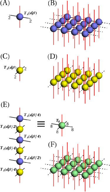
Figure 1: In A, the Trotter tensor $T_{x}(d\beta)$ with two spin indices (red lines) and two bond indices (black lines) along the $a$ axis. The bond indices have (bond) dimension $2$. In B, the gate $U_{XX}(d\beta)$ is a layer of tensors $T_{x}(d\beta)$ contracted through their bond indices. In C, $T_{z}(d\beta)$ with bond indices along the $b$ axis. In D, the gate $U_{ZZ}(d\beta)$ is a layer of $T_{z}(d\beta)$ contracted through their bond indices. In E, the six Trotter tensors contributing to the elementary time step $U(d\beta)$ in Eq. (9) can be merged into a single elementary Trotter tensor $T_{0}$ with a bond dimension $8$. In F, the time step $U(d\beta)$ is a layer of tensors $T_{0}$.

To rearrange $U(d\beta)$ as a tensor network, at every bond in Eqs. (7) we make a singular value decomposition

$$e^{\frac{d\beta}{8}X_{j}X_{j^{\prime}}} = \sum_{\mu=0,1}x_{j,\mu}~{}x_{j^{\prime},\mu},$$

$$e^{\frac{d\beta}{8}Z_{j}Z_{j^{\prime}}} = \sum_{\mu=0,1}z_{j,\mu}~{}z_{j^{\prime},\mu}.$$ (10)

Here $\mu$ is a bond index, $x_{j,\mu}\equiv\sqrt{\Lambda_{\mu}}\,(X_{j})^{\mu}$, and $z_{j,\mu}\equiv\sqrt{\Lambda_{\mu}}\,(Z_{j})^{\mu}$. The singular values are $\Lambda_{0}=\cosh\frac{d\beta}{8}$ and $\Lambda_{1}=\sinh\frac{d\beta}{8}$. Now we can write

$$U_{XX}(d\beta) = \sum_{\{\mu\}}\prod_{j}\left(\prod_{j^{\prime}}x_{j,\mu_{\langle j,j^{\prime}\rangle}}\right).$$ (11)

Here $\mu_{\langle j,j^{\prime}\rangle}$ is a bond index for the NN bond $\langle j,j^{\prime}\rangle$ along $a$ axis, and $\{\mu\}$ is a set of all such bond indices. The brackets enclose a Trotter tensor $T_{x}(d\beta)$ at site $j$, see Fig. 1A. It is a spin operator depending on bond indices connecting its site with its two NNs along the $a$ axis. A contraction of these Trotter tensors is the gate $U_{XX}(d\beta)$ in Fig. 1B. In a similar way,

$$U_{ZZ}(d\beta) = \sum_{\{\mu\}}\prod_{j}\left(\prod_{j^{\prime}}z_{j,\mu_{\langle j,j^{\prime}\rangle}}\right).$$ (12)

Here the brackets enclose a Trotter tensor $T_{z}(d\beta)$ at site $j$, shown in Fig. 1C. A layer of these Trotter tensors is the gate $U_{ZZ}(d\beta)$ in Fig. 1D.

To represent the time step (9) in Fig. 1E, six Trotter tensors are contracted along imaginary time into an elementary Trotter tensor $T_{0}$. Along each bond there are $3$ bond indices of dimension $2$ that are combined into a single one of dimension $8$. A layer of $T_{0}$ in Fig. 1F is the time step (9).

The evolution operator is a product of $N$ such elementary time steps,

$$U(\beta)=\left[U(d\beta)\right]^{N},$$ (13)

where $N=\beta/d\beta$ is a number of time steps. So far the only approximation is the Suzuki-Trotter decomposition.

III.3 Coarse graining and renormalization in imaginary time

Equation (13) suggests to combine $N$ elementary tensors $T_{0}$’s into a single PEPO tensor in a similar way as in Fig. 1E the six Trotter tensors were combined into a single $T_{0}$. Unfortunately, along each bond this would require to combine $N$ bond indices of dimension $8$ into a single one of dimension $8^{N}$. To prevent this exponential blow-up with $N$, we proceed step by step each time combining just two tensors into one: $T_{0}\times T_{0}\to T_{1}$,…,$T_{n-1}\times T_{n-1}\to T_{n}$. Here

$$n=\log_{2}N=\log_{2}\frac{\beta}{d\beta}$$ (14)

is the total number of the coarse-graining transformations that is only logarithmic in the total number of Suzuki-Trotter steps $N$ (and logarithmic in the small time step $d\beta$). After each step, $T_{m-1}\times T_{m-1}\to T_{m}$, the combined bond indices are renormalized down to $D$ by isometries $W_{m}$. The indices along the $a$ axis are renormalized by isometries $W^{x}_{m}$ and those along the $b$ axis by $W^{z}_{m}$, see Fig. 2A. Figure 3 shows the net outcome after $m=3$ coarse-graining transformations. Along each bond there are $3$ layers of isometries, from $W_{1}$ to $W_{3}$, that combine into a tree tensor network (TTN) TTN .

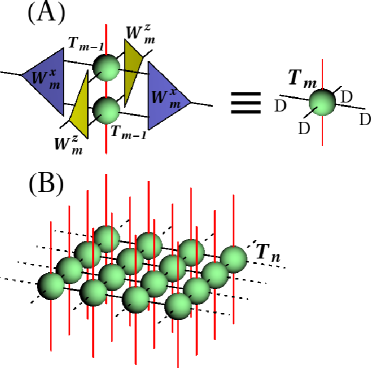
Figure 2: In A, the coarse-graining step along the imaginary time. Two Trotter tensors $T_{m-1}$ are combined and then renormalized into a single tensor $T_{m}$. The renormalization is made by isometries $W_{m}^{x}$ and $W_{m}^{z}$ on the bonds along the $a$ axis and $b$ axis, respectively. In B, after $n$ coarse-graining tranformations the PEPO tensor $T_{n}$ is obtained. A layer of contracted $T_{n}$ makes the PEPO Ansatz for the gate $U(\beta)$. It is equivalent to the PEPS Ansatz for the purification $|\psi(\beta)\rangle$ when its bottom spin indices are reinterpreted as ancilla indices.

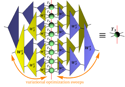
Figure 3: Three coarse-graining transformations result in the Trotter tensor $T_{3}$. The isometries acting along a given bond combine into a tree tensor network (TTN). They are optimized by repeated up- and down-sweeps.

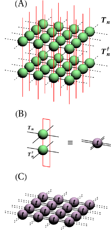
Figure 4: In A, the operator $e^{-\beta H}$ obtained after combining the two gates $U(\beta)$ and $U^{\dagger}(\beta)$ in Fig. 2B according to Eq. (6). Here the layers of tensors $T_{n}$ and $T_{n}^{\dagger}$ represent $U(\beta)$ and $U^{\dagger}(\beta)$ respectively. In B, two tensors $T_{n}$ combine into a transfer tensor $t$. In C, a layer of contracted transfer tensors is the partition function $Z={\rm Tr}e^{-\beta H}$.

A layer of $T_{n}$ shown in Fig. 2B is the PEPO Ansatz for the gate $U(\beta)$. When its bottom spin indices are reinterpreted as ancilla indices it becomes a PEPS Ansatz for the purification $|\psi(\beta)\rangle$. Figure 4A shows how to combine two gates $U(\beta)$ into the Gibbs operator $e^{-\beta H}$ according to Eq. (6). A single layer of transfer tensors $t$ in Figs. 4B and 4C is an Ansatz for the partition function $Z={\rm Tr}~{}e^{-\beta H}$.

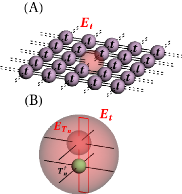
Figure 5: In A, the tensor environment $E_{t}$ for the tensor $t$ obtained after removing one tensor $t$ from the partition function in Fig. 4C. In B, tensor environment $E_{T_{n}}$ for the PEPO tensor $T_{n}$ obtained from $E_{t}$.

III.4 Variational optimization

In order to optimize the isometries we need an efficient algorithm to calculate a tensor environment of each isometry. A tensor environment of $W_{m}$ is the tensor $E_{W_{m}}$ that is generated by removing one $W_{m}$ from the partition function. It is proportional to the gradient $\partial Z/\partial W_{m}$. The algorithm proceeds step by step down the hierarchy of isometries.

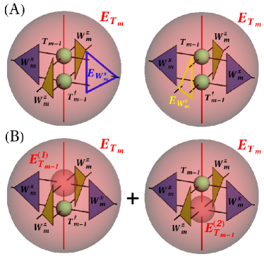
Figure 6: In A, the environments of the isometries $W_{m}^{x}$ and $W_{m}^{z}$ are obtained from $E_{T_{m}}$. In B, the step from the environment $E_{T_{m}}$ down to $E_{T_{m-1}}$. There are two inequivalent contributions to $E_{T_{m-1}}$. They add up to $E_{T_{m-1}}=E_{T_{m-1}}^{(1)}+E_{T_{m-1}}^{(2)}$.

A preparatory step is calculation of an environment $E_{t}\propto\partial Z/\partial t$ of the transfer tensor $t$ in Fig. 5A. It is the tensor that remains after removing one transfer tensor from the partition function in Fig. 4C. The infinite network $E_{t}$ cannot be contracted exactly, but its accurate approximation, that can be improved in a systematic way by increasing a control parameter $M$, can be obtained with the corner matrix renormalization (CMR) CMR described in Appendix A. Once converged, $E_{t}$ is contracted with one $T_{n}$ to yield an environment $E_{T_{n}}$ of the PEPO tensor $T_{n}$, see Fig. 5B. With $E_{T_{n}}$ we can initialize a down optimization sweep.

From $E_{T_{n}}$ we obtain the environments $E_{W_{n}^{x}}$ and $E_{W_{n}^{z}}$, see Fig. 6A. These environments are used immediately to update their isometries, see Fig. 7. With the updated $W_{n}$ we can calculate $E_{T_{n-1}}$, see Fig. 6B. From $E_{T_{n-1}}$ we obtain the environments $E_{W_{n-1}}$ and use them immediately to update the isometries $W_{n-1}$. The same procedure is repeated all the way down to $W_{1}$ whose update completes the down-sweep.

Once $W_{1}$ were updated, an up optimization sweep begins. It has $n$ steps. In the $m$-th step two tensors $T_{m-1}$ and the environment $E_{T_{m}}$ — calculated before during the down-sweep — are contracted to obtain the environments $E_{W_{m}}$ and update the isometries $W_{m}$, see Fig. 6B. The updated $W_{m}$ are used to coarse-grain $T_{m-1}\times T_{m-1}\to T_{m}$, see Fig. 2A. This basic step is repeated all the way up to $T_{n}$.

The up-sweep completes one optimization loop consisting of three stages:

• the CMR procedure:

  $$T_{n}\,\stackrel{{\scriptstyle\rm CMR}}{{\longrightarrow}}\,E_{t}\to\,E_{T_{n}};$$

• the down-sweep:

  $$E_{T_{n}}\to\,E_{W_{n}}\to\,E_{T_{n-1}}\to\dots\to\,E_{T_{1}}\to\,E_{W_{1}};$$

• the up-sweep:

  $$T_{0}\to\,E_{W_{1}}\to\,T_{1}\to\dots\to\,T_{n-1}\to\,E_{W_{n}}\to\,T_{n}.$$

Here each $E_{W_{m}}$ is used immediately to update $W_{m}$. The loop is repeated until convergence.

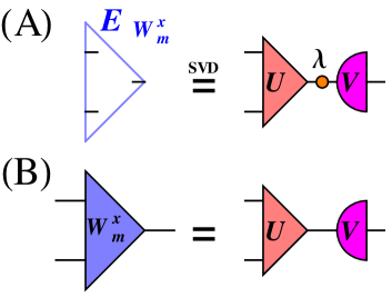
Figure 7: The update of the isometry $W^{x}_{m}$. In A, the isometric environment is subject to a singular value decomposition (SVD), $E_{W^{x}_{m}}=U\lambda V^{\dagger}$. In B, the isometry is updated as $W_{m}^{x}=UV^{\dagger}$. A similar procedure is applied to $W^{z}_{m}$.

The numerical cost of all the procedures in this Section scales like $D^{8}$. Typically, it is sub-leading as compared to the cost of CMR in Appendix A. Having thus outlined the algorithm we can proceed now with the results obtained for the 2D quantum compass model (1).

IV Results

IV.1 Order parameter and its susceptibility

The mean extrapolated values of the order parameter in the symmetry-broken phase were fitted with the scaling function

$$Q({\cal T})\propto({\cal T}_{c}-{\cal T})^{\beta},$$ (15)

where $\beta$ stands here for the critical exponent of the order parameter (this notation is widely accepted and we use it in this Section only). In this way the critical temperature was estimated as ${\cal T}_{c}=0.06090$, where the number of digits indicates precision of the linear fit alone. The exponent was estimated here as $\beta=0.223$ that is close but somewhat removed from the exact $\beta=1/8$.

In the symmetric phase on the other side of the transition, the mean extrapolated values of the linear susceptibility were fitted with

$$\chi({\cal T})\propto({\cal T}-{\cal T}_{c})^{\gamma},$$ (16)

where $\gamma$ is the susceptibility exponent. The susceptibility is defined as

$$\chi=\left.\frac{dQ}{dA}\right|_{A=0},$$ (17)

where $A$ is the anisotropy of the coupling constants in Eq. (1): $J_{x}=1+A/2$ and $J_{z}=1-A/2$. The derivative (17) was approximated accurately by a finite difference between $A=10^{-5}$ and $A=0$. The fit (16) yields ${\cal T}_{c}=0.06021$ and $\gamma=1.35$. The exponent is again somewhat removed from the exact $\gamma=1.75$. The estimate of ${\cal T}_{c}$ is close to that obtained from the order parameter on the other side of the critical point.

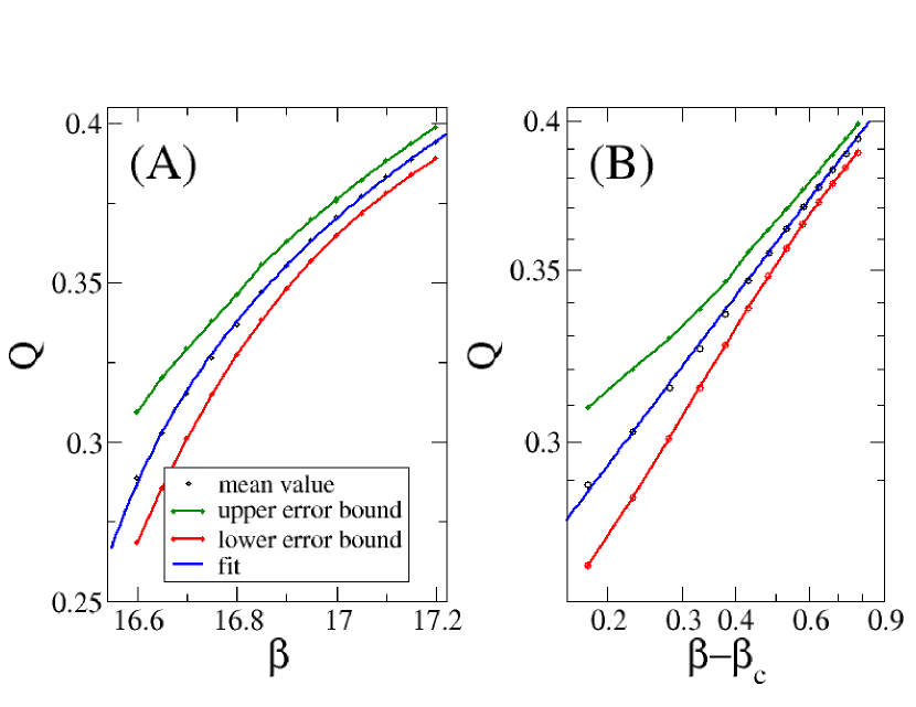
Figure 8: In (A), the order parameter $Q$ in Eq. (2) in the symmetry-broken phase near the phase transition. The mean value was obtained by extrapolation of the renormalization error to $0$, see Appendix B and Fig. 10. The error bounds show the errors of the extrapolation. The mean value was fitted with $Q\propto({\cal T}_{c}-{\cal T})^{\beta}$, where $\beta=0.223$ is the order parameter exponent and the critical temperature ${\cal T}_{c}=0.06090$. In (B), a log-log plot of the mean value and the best fit.

Relatively large errors of the critical exponents $\beta$ and $\gamma$ originate from estimates made relatively far from the critical point. Due to the non-analiticity at the critical point, even a tiny error in the estimate of ${\cal T}_{c}$ translates into a large error of a critical exponent.

Figures 8 and 9 show the order parameter and its linear susceptibility as a function of inverse temperature $\beta$ in the symmetry-broken and symmetric phases, respectively. The results are converged in the environmental bond dimension for $M\leq 40$, but they are not quite converged in the bond dimension $D\leq 15$. As explained in Appendix B, instead of the straightforward extrapolation with $1/D\to 0$, it is more reliable to make a smoother extrapolation with the actual error inflicted by the finite $D$. What is more, we found that an extrapolation with only the dominant error $e_{z}\to 0$ is smoother [we recall that $Q>0$ by our convention (2)]. We expect that, at least away from the critical point, physical quantities are analytical in $e_{z}$ and, consequently, for small enough $e_{z}$ they become linear. This expectation is confirmed by our data. Examples of linear fits used for the extrapolation are shown in Figs. 10 and 11. These fits include data for $D=8,\dots,15$. For some $D$ there are more than one data points corresponding to different random tensors used to initialize the variational optimization. Since $e_{z}$ does not capture all relevant errors — for instance, it does not control the accuracy of the environmental tensors — it is not justified to keep only the smallest $e_{z}$ for each $D$. The quality of the linear fits decreases when the critical point is approached from either side.

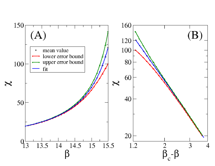
Figure 9: In (A), the linear susceptibility $\chi$ in (16) of the order parameter in the symmetric phase. The mean value was obtained by extrapolation of the renormalization error to $0$, see Appendix B and Fig. 11. The error bounds show the errors of the extrapolation. The mean was fitted with $\propto({\cal T}-{\cal T}_{c})^{\gamma}$, where $\gamma=1.35$ is the susceptibility exponent and ${\cal T}_{c}=0.06021$. In (B), a log-log plot of the mean value and the best fit.

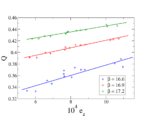
Figure 10: Three examples of the extrapolation of the order parameter $Q$ (2) described in Appendix B, to the vanishing renormalization error, $e_{z}\to 0$. Here the decreasing $e_{z}$ corresponds to increasing $D=8,\dots,15$. The results are converged for the regime of $M\leq 40$. The quality of the linear fit decreases with $\beta$ decreasing towards the phase transition. Each fit is used to extrapolate to $e_{z}=0$ and estimate the errors of the extrapolation. The means and error bounds are shown in Fig. 8.

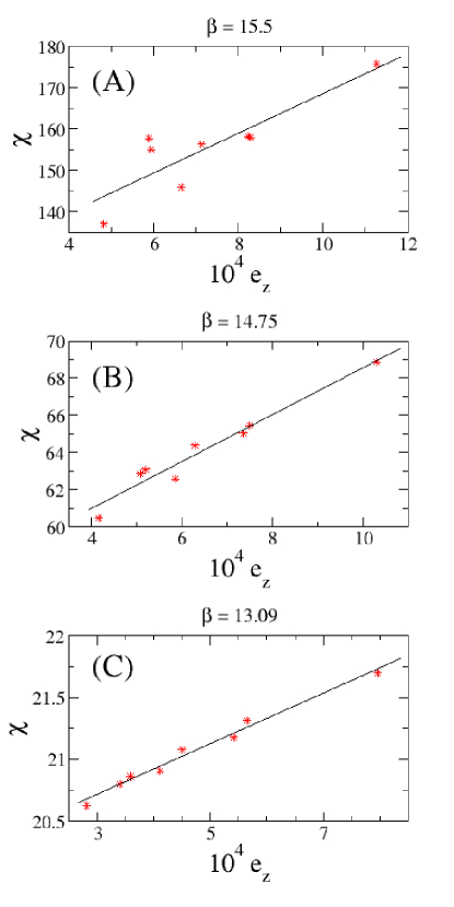
Figure 11: Three examples of the extrapolation of the susceptibility, described in Appendix B, to the vanishing renormalization error, $e_{z}\to 0$, for: (A) $\beta=15.5$, (B) $\beta=14.75$, and (C) $\beta=13.09$. Here the decreasing $e_{z}$ corresponds to increasing $D=8,\dots,15$. The results are converged for the regime of $M\leq 40$. The quality of the linear fit deteriorates with $\beta$ increasing towards the phase transition. Each fit is used to extrapolate to $e_{z}=0$ and to estimate the errors of this extrapolation, shown together with the mean value in Fig. 9.

The two estimates can be combined into a rough confidence interval ${\cal T}_{c}\in[0.0602,0.0609]$, or equivalently ${\cal T}_{c}\simeq 0.0606(4)$, giving a better idea of the actual error of the method than the tiny errors of the linear fits alone. Our result agrees well with the most reliable quantum Monte Carlo estimate ${\cal T}_{c}=0.0585(3)$, see Ref. Wen10 .

IV.2 Spin-spin correlation functions

In agreement with predictions for any finite temperature Nus15 , but in contrast with quantum Monte Carlo Wen10 , we find zero spontaneous magnetization,

$$\langle X_{m}\rangle=0=\langle Z_{m}\rangle,$$ (18)

within the numerical precision of $10^{-5}$. There is neither any local magnetization nor any long-range order in the spin-spin correlators.

The spin-spin correlations in the symmetry broken phase at $\beta=17.2$ are shown in Fig. 12. The dominant correlation function along the $a$ axis is exponential but relatively long-ranged with a correlation length estimated at $\xi=40(2)$. The transverse correlations decay exponentially on a much shorter transverse correlation length estimated at $\xi=6.9(4)$.

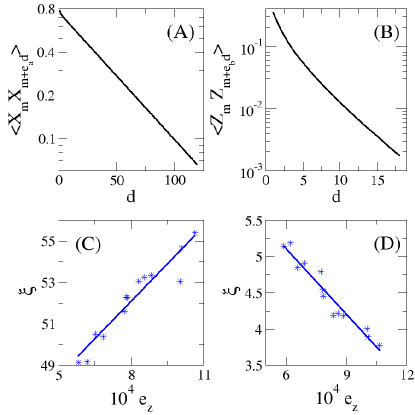
Figure 12: Top — spin correlations for increasing distance $d$: (A) the dominant correlation function $\langle X_{m}X_{m+e_{a}d}\rangle$ along the $a$ axis obtained for $D=15$ and converged in $M$ for $M=40$, and (B) the transverse correlation function $\langle Z_{m}Z_{m+e_{b}d}\rangle$ along the $b$ axis obtained for $D=15$ and converged in $M$ for $M=60$. Bottom — (C) the dominant correlation length $\xi$ as a function of the error estimate for different $D$. The extrapolation to zero error gives $\xi=40(2)$, and (D) the transverse correlation length $\xi$ as a function of the error. The extrapolation gives $\xi=6.9(4)$.

IV.3 Numerical details

All calculations were done in Matlab with an extensive use of the ncon procedure encon . They were checked for convergence in the elementary time step $d\beta\leq 0.005$. The number of isometric layers was fixed at $n=12$ with the number of time steps $N=2^{n}=4096$. To give an idea of the actual time and computer resources needed to perform the algorithm, the most challenging data points nearest to the phase transition at $\beta=15.5$ and $\beta=16.6$, with the highest bond dimensions $D=15$ and $M=40$, required $1-2$ days on a desktop. This time was needed to reach good convergence after $\sim 10^{2}$ iterations of the optimization loop. In each loop the CMR procedure made tens of iterations to converge the environmental tensors.

At $\beta=15.5$ and $\beta=16.6$, the calculations with $D=15$ were initialized by embedding converged tensors with smaller $D$ and the tensors with the smallest $D=8,\dots,10$ were converged after initialization with random numbers. At each point $100$ simulations with random initialization were preformed to exclude other solutions. The calculations farther away from criticality were initialized with tensors converged closer to it. Additionally, for $D=8,\dots,10$ at $\beta=15,14.5,14,13.5,13$ and $17.2,17.0,16.8,16.7$ further random initializations were performed — $100$ each time — to exclude other solutions. The further away form the phase transition, the fewer iterations were necessary to reach convergence.

V Conclusion

Table 1: Estimates of the critical temperature ${\cal T}_{c}$ for the 2D isotropic quantum compass model with $J_{x}=J_{z}=1$ as obtained by different methods, see Eq. (1).

	${\cal T}_{c}$	method	Ref.
	0.0625	high-$T$ expansion	Oit11
	0.075(2)	Trotter QMC	Tanaka
	0.055(1)	QMC periodic BC	Wen08
	0.0585(3)	QMC screw BC	Wen10
	0.0606(4)	VTNR	this work

We applied the variational tensor network renormalization (VTNR) in imaginary time, first introduced in Ref. var , to the 2D quantum compass model demonstrating its applicability beyond the quantum Ising model, in a model of interacting pseudospins close to geometric frustration. The method makes efficient use of the bond dimension and it is only logarithmic in the total number of Suzuki-Trotter imaginary time steps. An important new algorithmic feature is the extrapolation in the small error inflicted by the finite bond dimension $D$.

The presented VTNR reproduces the thermodynamic phase transition in the 2D quantum compass model. In the symmetry broken phase at ${\cal T}<{\cal T}_{c}$, we find nematic order with long-range spin correlations along the dominant axis, and short-range correlations in the transverse direction, but no spontaneous magnetization. We also attempted to estimate the order parameter exponent $\beta=0.224$ and the susceptibility exponent $\gamma=1.35$ that are close but somewhat removed from the exact values $\beta=0.125$ and $\gamma=1.75$, respectively.

The present approach provides a controlled estimate of the critical temperature at ${\cal T}_{c}=0.0606(4)$. In Table 1 we compare this result with earlier estimates including the most recent QMC Wen10 with screw boundary conditions (BC). These BC remove anomalous scalings observed in the case of periodic BC without introducing the sign problem making Ref. [55] the most reliable benchmark. Our estimate at $3.5\%$ above their ${\cal T}_{c}=0.0585(3)$ is in good agreement with QMC. The accuracy of QMC is limited by extrapolation to infinite system size while the accuracy of our infinite tensor network by extrapolation to infinite bond dimension. This positive test suggests that the method used here could be a competitive tool to treat systems suffering from the sign problem.

Appendix A Corner matrix renormalization

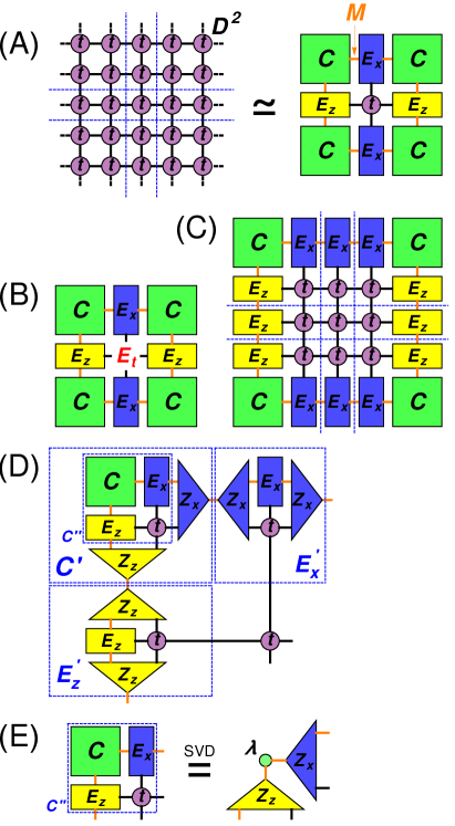
Figure 13: In A, planar version of the partition function in Fig. 4C. From the point of view of the central tensor $t$, this infinite network can be replaced by a finite effective one made of a corner matrix $C$ and edge tensors $E_{x}$ and $E_{z}$. Each of them represents its corresponding infinite sector delimited by the blue dashed lines. The environmental tensors contract through bond indices of dimension $M$. In B, the finite effective environment $E_{t}$ made of the finite environmental tensors. With increasing $M$ it becomes the exact one in Fig. 5A. In C, a network equivalent to the networks in panel A. Here the blue dashed lines separate enlarged environmental tensors. In D, the enlarged tensors are renormalized by isometries $Z_{x}$ and $Z_{z}$ to new tensors $C^{\prime}$, $E^{\prime}_{x}$ and $E^{\prime}_{z}$ back with the environmental bond dimension $M$. In E, the isometries are obtained from a singular value decomposition (SVD) of the enlarged corner: $C^{\prime\prime}=Z_{z}\lambda Z_{x}^{\dagger}$.

An infinite network, like the one in Fig. 4C, cannot be contracted exactly but, fortunately, what we often need is not this number, but a tensor environment for a few sites of interest like, for instance, the environment $E_{t}$ in Fig. 5A. From the point of view of the removed $t$, its exact infinite environment can be substituted with a finite effective one made of finite corner matrices $C$ and edge tensors $E_{x}$ and $E_{z}$, see Fig. 13. The environmental tensors $C$ and $E$ are contracted with each other by environmental bond indices of dimension $M$. By increasing $M$ the effective $E_{t}$ can be converged towards the exact one in a systematic way. When the correlation length is finite the convergence is reached exponentially at a finite $M$. At a critical point, even though the correlation length $\xi(M)$ remains finite for any finite $M$, it quickly diverges with a power of $M$ making local observables and correlations up to the distance $\xi(M)$ converge to their exact values self ; var .

The finite tensors $C$ and $E$ represent infinite sectors of the network in Fig. 13A. The tensors are converged by iterating the corner matrix renormalization in Figs. 13C-E. In every renormalization step, the corner $C$ is enlarged to $C^{\prime\prime}$. This operation represents the top-left corner sector in Fig. 13A absorbing one more layer of tensors $t$. The enlarged $C^{\prime\prime}$ is subject to singular value decomposition $C^{\prime\prime}=Z_{z}\lambda Z_{x}^{\dagger}$, see Fig. 13E. $\lambda$ is truncated to $M$ largest singular values and the unitaries $Z_{z}$ and $Z_{x}$ to the corresponding isometries. The isometries renormalize $C^{\prime\prime}$ and the enlarged edge tensors to a new corner $C^{\prime}$ and edges $E^{\prime}$, respectively. The whole procedure is iterated until convergence.

The numerical cost of converging the environmental tensors is ${\cal O}\left[M^{3}(D^{2})^{3}\right]$, where $D^{2}$ is the bond dimension of $t$. The cost of calculating $E_{T_{n}}$ can be reduced to ${\cal O}\left(M^{2}D^{6},M^{3}D^{4}\right)$ if one goes directly from the environmental tensors to $E_{T_{n}}$ without calculating the intermediate $E_{t}$.

Appendix B Error estimate

Observables should be converged not only in $M$ but also in $D$. A modest $D\simeq 7$ is sufficient in the 2D quantum Ising model var , but in realistic models rather than full convergence we would expect to get close enough to it to make a reliable extrapolation with $1/D\to 0$. However, the raw $1/D$ may be not the most reliable small parameter for the extrapolation CorbozHubbard . For instance, the PEPO Ansatz may not change much between $D$ and $D+1$ but then suddenly improve for $D+2$ making the dependence of observables on $1/D$ rough. A more direct measure of the actual error inflicted by a finite $D$ would make the dependence smoother and the extrapolation more reliable.

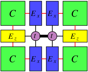
Figure 14: The network used to estimate the error along the central $a$-bond inflicted by the isometries $W^{x}_{m}$ with the bond dimension $D$. Its contraction is a number $N^{x}_{D}$. When the bond dimension of the isometries on the central bond is enlarged to $D^{\prime}>D$ and the enlarged isometries on this bond are optimized the number becomes $N^{x}_{D^{\prime}}$. For large enough $D^{\prime}$ it converges to $N^{x}_{\infty}$. The relative error $e_{x}$ is given by Eq. (19).

The measure can be constructed in a similar way as for the zero-temperature PEPS CorbozHubbard . Figure 14 shows the network used to estimate the error inflicted by the isometries $W^{x}$ with the bond dimension $D$. This network is a number $N^{x}_{D}$. When the bond dimension of the isometries on the central bond is enlarged to $D^{\prime}>D$ and the enlarged isometries on this bond are optimized, then the number becomes $N^{x}_{D^{\prime}}$. It converges to $N^{x}_{\infty}$ for a large enough $D^{\prime}$. In our calculations $D^{\prime}=4D$ proved to be sufficient. The relative error is given by

$$e_{x}(D)=(N^{x}_{\infty}-N^{x}_{D})/N^{x}_{\infty}.$$ (19)

In a similar way we obtain the error inflicted by isometries $W^{z}$ on a bond along the $b$ axis:

$$e_{z}(D)=(N^{z}_{\infty}-N^{z}_{D})/N^{z}_{\infty}.$$ (20)

Appendix C Figure of merit

The algorithm optimizes each isometry $W^{x}_{m}$ to maximize its overlap with its environment $E_{W^{x}_{m}}$. As the overlap is proportional to the partition function $Z$, the optimization aims at maximizing $Z$. We will argue that in the compass model maximizing $Z$ is equivalent to minimizing the error inflicted on $Z$ by the isometry.

Indeed, the $n$ layers of isometries $W^{x}_{1}$,…,$W^{x}_{n}$ make a tree tensor network like the one shown in Fig. 3 in case of $n=3$ layers. The whole TTN is also an isometry to be called $W_{x}$. (We note in passing that in principle the TTN could be replaced with a more general tensor network like the one in Ref. ramsetal , but it is not clear at the time of writing how to perform its variational optimization with full tensor environment.) In the PEPO Ansatz for the gate $U(\beta)$ in Fig. 2B on every bond along the $a$ axis there are two isometries $W_{x}$ that combine into a projector $P_{x}=W_{x}W_{x}^{\dagger}$. We want to minimize the error inflicted on the partition function by $P_{x}$.

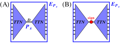
Figure 15: In A, $n$ layers of isometries $W^{x}_{1}$,…,$W^{x}_{n}$ make a TTN, see Fig. 3 in case of $n=3$ layers. The TTN is also an isometry to be called $W_{x}$. Two TTNs make a projector $P_{x}=W_{x}W^{\dagger}_{x}$. In B, the sign matrix (22) is inserted into the central bond. After this insertion the isometries $W^{x}_{m}$ can be updated by maximizing their overlaps with their respective environments even when $E_{P_{x}}$ is not positive-semidefinite.

The partition function in Fig. 4 can be represented by the effective network in Fig. 14. We focus on the two projectors $P_{x}$ on the central bond, one in each of the two layers $U(\beta)$. Given the left-right symmetry of this network reflecting the symmetry of the compass model, it can be shown that $E_{P_{x}}={\cal M}{\cal M}^{\dagger}$, where ${\cal M}$ is a huge matrix representing the left half of Fig. 14. The environment is symmetric and positive-semidefinite, hence the partition function is distorted least by the projector $P_{x}$ that maximizes its contraction with $E_{P_{x}}$, see Fig. 15. This optimal projector is made of isometries that in turn maximize their overlaps with the respective environments.

In order to put this simple result in a more general context, let us consider now $E_{P_{x}}$ that is not positive-semidefinite but is still symmetric. Since the $P_{x}$ to be contracted with $E_{P_{x}}$ is symmetric, hence only the symmetric part of $E_{P_{x}}$ matters anyway. Now the least distortive projector is no longer the one on the largest eigenvalues of $E_{P_{x}}$, but that on the eigenvalues with the largest magnitudes. The huge $E_{P_{x}}$ can be neither diagonalized nor even calculated, but the $D\times D$ matrix $e_{P_{x}}$ obtained after cutting the central $D$-bond in Fig. 15 is $E_{P_{x}}$ projected on a $D$-dimensional subspace. This matrix can be efficiently calculated and diagonalized,

$$e_{P_{x}}=\sum_{\alpha=1}^{D}|\alpha\rangle\lambda_{\alpha}\langle\alpha|,$$ (21)

and we can construct its sign operator,

$${\rm sign}\left(e_{P_{x}}\right)=\sum_{\alpha=1}^{D}|\alpha\rangle\,{\rm sign}\left(\lambda_{\alpha}\right)\langle\alpha|.$$ (22)

Inserting this sign into the cut $D$-bond in Fig. 15 is equivalent to replacing the eigenvalues of $E_{P_{x}}$ by their magnitudes. With the inserted sign, the least distortive isometries $W^{x}_{m}$ are again those that maximize their overlaps with their respective environments. The sign insertion is a redundant null operation when $E_{P_{x}}\geq 0$, like in the quantum compass or quantum Ising models, but it proves essential in the fermionic Hubbard model Cza16 .

References

- (1) Bruce Normand, Cont. Phys. 50, 533 (2009).
- (2) Leon Balents, Nature (London) 464, 199 (2010).
- (3) J. Villain, J. Phys. C: Solid State Phys. 10, 1717 (1977).
- (4) L. Longa and A. M. Oleś, J. Phys. A: Math. Theor. 13, 1031 (1980).
- (5) L. Amico, R. Fazio, A. Osterloh, and V. Vedral, Rev. Mod. Phys. 80, 517 (2008).
- (6) Z. Nussinov and J. van den Brink, Rev. Mod. Phys. 87, 1 (2015).
- (7) K. I. Kugel and D. I. Khomskii, JETP 37, 725 (1973); Sov. Phys. Usp. 25, 231 (1982).
- (8) L. F. Feiner, A. M. Oleś, and J. Zaanen, Phys. Rev. Lett. 78, 2799 (1997); J. Phys.: Condens. Matter 10, L555 (1998).
- (9) A. M. Oleś, G. Khaliullin, P. Horsch, and L. F. Feiner, Phys. Rev. B 72, 214431 (2005).
- (10) G. Khaliullin, Prog. Theor. Phys. Suppl. 160, 155 (2005).
- (11) C. Ulrich, A. Gössling, M. Grüninger, M. Guennou, H. Roth, M. Cwik, T. Lorenz, G. Khaliullin, and B. Keimer, Phys. Rev. Lett. 97, 157401 (2006); C. Ulrich, G. Khaliullin, M. Guennou, H. Roth, T. Lorenz, and B. Keimer, ibid. 115, 156403 (2015).
- (12) F. Krüger, S. Kumar, J. Zaanen, and J. van den Brink, Phys. Rev. B 79, 054504 (2009).
- (13) P. Corboz, M. Lajkó, A. M. Laüchli, K. Penc, and F. Mila, Phys. Rev. X 2, 041013 (2012).
- (14) K. Wohlfeld, M. Daghofer, S. Nishimoto, G. Khaliullin, and J. van den Brink, Phys. Rev. Lett. 107, 147201 (2011); P. Marra, K. Wohlfeld, and J. van den Brink, ibid. 109, 117401 (2012); V. Bisogni, K. Wohlfeld, S. Nishimoto, C. Monney, J. Trinckauf, K. Zhou, R. Kraus, K. Koepernik, C. Sekar, V. Strocov, B. Büchner, T. Schmitt, J. van den Brink, and J. Geck, ibid. 114, 096402 (2015); E. M. Plotnikova, M. Daghofer, J. van den Brink, and K. Wohlfeld, ibid. 115, 106401 (2016); K. Wohlfeld, S. Nishimoto, M. W. Haverkort, and J. van den Brink, Phys. Rev. B 88, 195138 (2013); C.-C. Chen, M. van Veenendaal, T. P. Devereaux, and K. Wohlfeld, ibid. 91, 165102 (2015).
- (15) W. Brzezicki, J. Dziarmaga, and A. M. Oleś, Phys. Rev. Lett. 109, 237201 (2012); Phys. Rev. B 87, 064407 (2013); W. Brzezicki and A. M. Oleś, ibid. 83, 214408 (2011); P. Czarnik and J. Dziarmaga, ibid. 91, 045101 (2015).
- (16) W. Brzezicki, A. M. Oleś, and M. Cuoco, Phys. Rev. X 5, 011037 (2015); W. Brzezicki, M. Cuoco, and A. M. Oleś, J. Sup. Novel Magn. 29, 563 (2016).
- (17) A. M. Oleś, J. Phys.: Condens. Matter 24, 313201 (2012); Acta Phys. Polon. A 127, 163 (2015).
- (18) G. Jackeli and G. Khaliullin, Phys. Rev. Lett. 102, 017205 (2009); J. Chaloupka, G. Jackeli, and G. Khaliullin, ibid. 105, 027204 (2010); 110, 097204 (2013).
- (19) J. van den Brink, P. Horsch, F. Mack, and A. M. Oleś, Phys. Rev. B 59, 6795 (1999).
- (20) J. van den Brink, New J. Phys. 6, 201 (2004).
- (21) T. Tanaka, M. Matsumoto, and S. Ishihara, Phys. Rev. Lett. 95, 267204 (2005); T. Tanaka and S. Ishihara, Phys. Rev. Lett. 98, 256402 (2007). .
- (22) A. van Rynbach, S. Todo, and S. Trebst, Phys. Rev. Lett. 105, 146402 (2010).
- (23) P. Wróbel and A. M. Oleś, Phys. Rev. Lett. 104, 206401 (2010); P. Wróbel, R. Eder, and A. M. Oleś, Phys. Rev. B 86, 064415 (2012).
- (24) M. Daghofer, K. Wohlfeld, A. M. Oleś, E. Arrigoni, and P. Horsch, Phys. Rev. Lett. 100, 066403 (2008); A. Nicholson, W. Ge, X. Zhang, J. Riera, M. Daghofer, A. M. Oleś, G. B. Martins, A. Moreo, and E. Dagotto, ibid. 106, 217002 (2011); M. Daghofer, A. Nicholson, A. Moreo, and E. Dagotto, Phys. Rev. B 81, 014511 (2010).
- (25) F. Trousselet, A. Ralko, and A. M. Oleś, Phys. Rev. B 86, 014432 (2012).
- (26) G. Chen and L. Balents, Phys. Rev. Lett. 110, 206401 (2013).
- (27) P. Milman, W. Maineult, S. Guibal, L. Guidoni, B. Douçot, L. Ioffe, and T. Coudreau, Phys. Rev. Lett. 99, 020503 (2007).
- (28) T. Tanaka and S. Ishihara, Phys. Rev. Lett. 98, 256402 (2007).
- (29) S. Wenzel and W. Janke, Phys. Rev. B 78, 064402 (2008).
- (30) F. Trousselet, A. M. Oleś, and P. Horsch, Europhys. Lett. 91, 40005 (2010); Phys. Rev. B 86, 134412 (2012).
- (31) P. Czarnik and J. Dziarmaga, Phys. Rev. B 92, 035152 (2015).
- (32) X. Chen and A. Vishwanath, Phys. Rev. X 5, 041034 (2015).
- (33) S. R. White, Phys. Rev. Lett. 69, 2863 (1992).
- (34) U. Schollwöck, Rev. Mod. Phys. 77, 259 (2005).
- (35) U. Schollwöck, Annals of Physics 326, 96 (2011).
- (36) F. Verstraete and J. I. Cirac, arXiv:cond-mat/0407066 (2004); V. Murg, F. Verstraete, and J. I. Cirac, Phys. Rev. A 75, 033605 (2007); G. Sierra and M. A. Martin-Delgado, arXiv:cond-mat/9811170 (1998); T. Nishino and K. Okunishi, J. Phys. Soc. Jpn. 67, 3066 (1998); Y. Nishio, N. Maeshima, A. Gendiar, and T. Nishino, arXiv:cond-mat/0401115 (2004); Z.-C. Gu, M. Levin, and X.-G. Wen, Phys. Rev. B 78, 205116 (2008); J. Jordan, R. Orús, G. Vidal, F. Verstraete, and J. I. Cirac, Phys. Rev. Lett. 101, 250602 (2008); H. C. Jiang, Z. Y. Weng, and T. Xiang, ibid. 101, 090603 (2008); Z. Y. Xie, H. C. Jiang, Q. N. Chen, Z. Y. Weng, and T. Xiang, ibid. 103, 160601 (2009); P.-C. Chen, C.-Y. Lai, and M.-F. Yang, J. Stat. Mech.: Theory Exp. (2009) P10001; R. Orús and G. Vidal, Phys. Rev. B 80, 094403 (2009).
- (37) G. Vidal, Phys. Rev. Lett. 99, 220405 (2007); 101, 110501 (2008); Ł. Cincio, J. Dziarmaga, and M. M. Rams, ibid. 100, 240603 (2008); G. Evenbly and G. Vidal, ibid. 102, 180406 (2009); 112, 240502 (2014); Phys. Rev. B 79, 144108 (2009); 89, 235113 (2014).
- (38) T. Barthel, C. Pineda, and J. Eisert, Phys. Rev. A 80, 042333 (2009); P. Corboz and G. Vidal, Phys. Rev. B 80, 165129 (2009); P. Corboz, G. Evenbly, F. Verstraete, and G. Vidal, Phys. Rev. A 81, 010303(R) (2010); C. V. Kraus, N. Schuch, F. Verstraete, and J. I. Cirac, ibid. 81, 052338 (2010); C. Pineda, T. Barthel, and J. Eisert, ibid. 81, 050303(R) (2010); Z.-C. Gu, F. Verstraete, and X.-G. Wen, arXiv:1004.2563 (2010).
- (39) P. Corboz, R. Orús, B. Bauer, and G. Vidal, Phys. Rev. B 81, 165104 (2010); P. Corboz, S. R. White, G. Vidal, and M. Troyer, ibid. 84, 041108 (2011); P. Corboz, T. M. Rice, and M. Troyer, Phys. Rev. Lett. 113, 046402 (2014).
- (40) P. Corboz, Phys. Rev. B 93, 045116 (2016).
- (41) S. Yan, D. A. Huse, and S. R. White, Science 332, 1173 (2011).
- (42) L. Cincio and G. Vidal, Phys. Rev. Lett. 110, 067208 (2013).
- (43) S.-J. Ran, W. Li, S.-S. Gong, A. Weichselbaum, J. von Delft, and Gang Su, arXiv:1508.03451 (2015).
- (44) D. Poilblanc, N. Schuch, D. Pérez-García, and J. I. Cirac, Phys. Rev. B 86, 014404 (2012).
- (45) D. Poilblanc and N. Schuch, Phys. Rev. B 87, 140407(R) (2013).
- (46) L. Wang, D. Poilblanc, Z.-C. Gu, X.-G. Wen, and F. Verstraete, Phys. Rev. Lett. 111, 037202 (2013).
- (47) F. Verstraete, J. J. Garcia-Ripoll, and J. I. Cirac, Phys. Rev. Lett. 93, 207204 (2004); M. Zwolak and G. Vidal, ibid. 93, 207205 (2004); A. E. Feiguin and S. R. White, Phys. Rev. B 72, 220401 (2005).
- (48) S. R. White, arXiv:0902.4475 (2009); E. M. Stoudenmire and S. R. White, New J. Phys. 12, 055026 (2010); I. Pizorn, V. Eisler, S. Andergassen, and M. Troyer, ibid. 16, 073007 (2014).
- (49) P. Czarnik, Ł. Cincio, and J. Dziarmaga, Phys. Rev. B 86, 245101 (2012); P. Czarnik and J. Dziarmaga, ibid. 90, 035144 (2014).
- (50) P. Czarnik and J. Dziarmaga, Phys. Rev. B 92, 035120 (2015).
- (51) A. Molnár, N. Schuch, F. Verstraete, and J. I. Cirac, Phys. Rev. B 91, 045138 (2015).
- (52) Z. Y. Xie, H. C. Jiang, Q. N. Chen, Z. Y. Weng, and T. Xiang, Phys. Rev. Lett. 103, 160601 (2009); H. H. Zhao, Z. Y. Xie, Q. N. Chen, Z. C. Wei, J. W. Cai, and T. Xiang, Phys. Rev. B 81, 174411 (2010); W. Li, S.-J. Ran, S.-S. Gong, Y. Zhao, B. Xi, F. Ye, and G. Su, Phys. Rev. Lett. 106, 127202 (2011); Shi-Ju Ran, Wei Li, Bin Xi, Zhe Zhang, and Gang Su, ibid. 86, 134429 (2012); S.-J. Ran, B. Xi, T. Liu, and G. Su, ibid. 88, 064407 (2013); A. Denbleyker, Y. Liu, Y. Meurice, M. P. Qin, T. Xiang, Z. Y. Xie, J. F. Yu, and H. Zou, Phys. Rev. D 89, 016008 (2014); H. H. Zhao, Z. Y. Xie, T. Xiang, and M. Imada, arXiv:1510.03333 (2015).
- (53) Z. Y. Xie, J. Chen, M. P. Qin, J. W. Zhu, L. P. Yang, and T. Xiang, Phys. Rev. B 86, 045139 (2012).
- (54) K. Takai, K. Ido, T. Misawa, Y. Yamaji, and M. Imada, arXiv:1510.05352 (2015).
- (55) S. Wenzel, W. Janke, and A. M. Läuchli, Phys. Rev. E 81, 066702 (2010).
- (56) J. Oitmaa and C. J. Hamer, Phys. Rev. B 83, 094437 (2011).
- (57) A. Mishra, M. Ma, Fu-Chun Zhang, S. Guertler, L.-H. Tang, and S. Wan, Phys. Rev. Lett. 93, 207201 (2004).
- (58) W. Brzezicki and A. M. Oleś, Phys. Rev. B 82, 060401 (2010); 87, 214421 (2013).
- (59) L. Tagliacozzo, G. Evenbly, and G. Vidal, Phys. Rev. B 80, 235127 (2009).
- (60) R. J. Baxter, J. Math. Phys. 9, 650 (1968); J. Stat. Phys. 19, 461 (1978); T. Nishino and K. Okunishi, J. Phys. Soc. Jpn. 65, 891 (1996); R. Orús and G. Vidal, Phys. Rev. B 80, 094403 (2009); R. Orús, ibid. 85, 205117 (2012); Ann. Phys. (N.Y.) 349, 117 (2014); Ho N. Phien, I. P. McCulloch, and G. Vidal, Phys. Rev. B 91, 115137 (2015).
- (61) R. N. C. Pfeifer, G. Evenbly, S. Singh, and G. Vidal, arXiv:1402.0939 (2014).
- (62) M. Bal, M. M. Rams, V. Zauner, J. Haegeman, and F. Verstraete, arXiv:1509.01522 (2015).
- (63) P. Czarnik and J. Dziarmaga, unpublished.