Computing the $L_{1}$ Geodesic Diameter and Center of a Polygonal Domain

Abstract

For a polygonal domain with $h$ holes and a total of $n$ vertices, we present algorithms that compute the $L_{1}$ geodesic diameter in $O(n^{2}+h^{4})$ time and the $L_{1}$ geodesic center in $O((n^{4}+n^{2}h^{4})\alpha(n))$ time, respectively, where $\alpha(\cdot)$ denotes the inverse Ackermann function. No algorithms were known for these problems before. For the Euclidean counterpart, the best algorithms compute the geodesic diameter in $O(n^{7.73})$ or $O(n^{7}(h+\log n))$ time, and compute the geodesic center in $O(n^{11}\log n)$ time. Therefore, our algorithms are significantly faster than the algorithms for the Euclidean problems. Our algorithms are based on several interesting observations on $L_{1}$ shortest paths in polygonal domains.

1 Introduction

A polygonal domain $\mathcal{P}$ is a closed and connected polygonal region in the plane $\mathbb{R}^{2}$, with $h\geq 0$ holes (i.e., simple polygons). Let $n$ be the total number of vertices of $\mathcal{P}$. Regarding the boundary of $\mathcal{P}$ as obstacles, we consider shortest obstacle-avoiding paths lying in $\mathcal{P}$ between any two points $p,q\in\mathcal{P}$. Their geodesic distance $d(p,q)$ is the length of a shortest path between $p$ and $q$ in $\mathcal{P}$. The geodesic diameter (or simply diameter) of $\mathcal{P}$ is the maximum geodesic distance over all pairs of points $p,q\in\mathcal{P}$, i.e., $\max_{p\in\mathcal{P}}\max_{q\in\mathcal{P}}d(p,q)$. Closely related to the diameter is the min-max quantity $\min_{p\in\mathcal{P}}\max_{q\in\mathcal{P}}d(p,q)$, in which a point $p^{*}$ that minimizes $\max_{q\in\mathcal{P}}d(p^{*},q)$ is called a geodesic center (or simply center) of $\mathcal{P}$. Each of the above quantities is called Euclidean or $L_{1}$ depending on which of the Euclidean or $L_{1}$ metric is adopted to measure the length of paths.

For simple polygons (i.e., $h=0$), the Euclidean geodesic diameter and center have been studied since the 1980s [3, 8, 23]. For the diameter, Chazelle [8] gave the first $O(n^{2})$-time algorithm, followed by an $O(n\log n)$-time algorithm by Suri [23]. Finally, Hershberger and Suri [15] gave a linear-time algorithm for computing the diameter. For the center, after an $O(n^{4}\log n)$-time algorithm by Asano and Toussaint [3], Pollack, Sharir, and Rote [21] gave an $O(n\log n)$ time algorithm for computing the geodesic center. Recently, Ahn et al. [1] solved the problem in $O(n)$ time.

For the general case (i.e., $h>0$), the problems are more difficult. The Euclidean diameter problem was solved in $O(n^{7.73})$ or $O(n^{7}(h+\log n))$ time [4]. The Euclidean center problem was first solved in $O(n^{12+\epsilon})$ time for any $\epsilon>0$ [5] and then an improved $O(n^{11}\log n)$ time algorithm was given in [24].

For the $L_{1}$ versions, the geodesic diameter and center of simple polygons can be computed in linear time [6, 22], but we are unaware of any previous algorithms for polygonal domains. In this paper, we present the first algorithms that compute the geodesic diameter and center of a polygonal domain $\mathcal{P}$ (as defined above) in $O(n^{2}+h^{4})$ and $O((n^{4}+n^{2}h^{4})\alpha(n))$ time, respectively, where $\alpha(\cdot)$ is the inverse Ackermann function. Comparing with the algorithms for the same problems under the Euclidean metric, our algorithms are much more efficient, especially when $h$ is significantly smaller than $n$.

As discussed in [4], a main difficulty of polygonal domains seemingly arises from the fact that there can be several topologically different shortest paths between two points, which is not the case for simple polygons. Bae, Korman, and Okamoto [4] observed that the Euclidean diameter can be realized by two interior points of a polygonal domain, in which case the two points have at least five distinct shortest paths. This difficulty makes their algorithm suffer a fairly large running time. Similar issues also arise in the $L_{1}$ metric, where a diameter may also be realized by two interior points (this can be seen by extending the examples in [4]).

We take a different approach from [4]. We first construct an $O(n^{2})$-sized cell decomposition of $\mathcal{P}$ such that the $L_{1}$ geodesic distance function restricted to any pair of two cells can be explicitly described in $O(1)$ complexity. Consequently, the $L_{1}$ diameter and center can be obtained by exploring these cell-restricted pieces of the geodesic distance. This leads to simple algorithms that compute the diameter in $O(n^{4})$ time and the center in $O(n^{6}\alpha(n))$ time. With the help of an “extended corridor structure” of $\mathcal{P}$ [9, 10, 11], we reduce the $O(n^{2})$ complexity of our decomposition to another “coarser” decomposition of $O(n+h^{2})$ complexity; with another crucial observation (Lemma 3.1), one may compute the diameter in $O(n^{3}+h^{4})$ time by using our techniques for the above $O(n^{4})$ time algorithm. One of our main contributions is an additional series of observations (Lemmas 3.4 to 4.15) that allow us to further reduce the running time to $O(n^{2}+h^{4})$. These observations along with the decomposition may have other applications as well. The idea for computing the center is similar.

We are motivated to study the $L_{1}$ versions of the diameter and center problems in polygonal (even non-rectilinear) domains for several reasons. First, the $L_{1}$ metric is natural and well studied in optimization and routing problems, as it models actual costs in rectilinear road networks and certain robotics/VLSI applications. Indeed, the $L_{1}$ diameter and center problems in the simpler setting of simply connected domains have been studied [6, 22]. Second, the $L_{1}$ metric approximates the Euclidean metric. Further, improved understanding of algorithmic results in one metric can assist in understanding in other metrics; e.g., the continuous Dijkstra methods for $L_{1}$ shortest paths of [18, 19] directly led to improved results for Euclidean shortest paths.

1.1 Preliminaries

For any subset $A\subset\mathbb{R}^{2}$, denote by $\partial A$ the boundary of $A$. Denote by $\overline{pq}$ the line segment with endpoints $p$ and $q$. The $L_{1}$ length of $\overline{pq}$ is defined to be $|x_{p}-x_{q}|+|y_{p}-y_{q}|$, where $x_{p}$ and $y_{p}$ are the $x$- and $y$-coordinates of $p$, respectively, and $x_{q}$ and $y_{q}$ are the $x$- and $y$-coordinates of $q$, respectively. For any polygonal path $\pi\in\mathbb{R}^{2}$, let $|\pi|$ be the $L_{1}$ length of $\pi$, which is the sum of the $L_{1}$ lengths of all segments of $\pi$. In the following, a path always refers to a polygonal path. A path is $xy$-monotone (or monotone for short) if every vertical or horizontal line intersects it in at most one connected component. Following is a basic observation on the $L_{1}$ length of paths in $\mathbb{R}^{2}$, which will be used in our discussion.

Fact 1.

For any monotone path $\pi$ between two points $p,q\in\mathbb{R}^{2}$, $|\pi|=|\overline{pq}|$ holds.

We view the boundary $\partial\mathcal{P}$ of our polygonal domain $\mathcal{P}$ as a series of obstacles so that no path in $\mathcal{P}$ is allowed to cross $\partial\mathcal{P}$. Throughout the paper, unless otherwise stated, a shortest path always refers to an $L_{1}$ shortest path and the distance/length of a path (e.g., $d(p,q)$) always refers to its $L_{1}$ distance/length. The diameter/center always refers to the $L_{1}$ geodesic diameter/center. For simplicity of discussion, we make a general position assumption that no two vertices of $\mathcal{P}$ have the same $x$- or $y$-coordinate.

The following will also be exploited as a basic fact in further discussion.

Fact 2 ([13, 14]).

In any simple polygon $P$, there is a unique Euclidean shortest path $\pi$ between any two points in $P$. The path $\pi$ is also an $L_{1}$ shortest path in $P$.

The rest of the paper is organized as follows. In Section 2, we introduce our cell decomposition of $\mathcal{P}$ and exploit it to have preliminary algorithms for computing the diameter and center of $\mathcal{P}$. The algorithms will be improved later in Section 4, based on the extended corridor structure and new observations discussed in Section 3. One may consider the preliminary algorithms in Section 2 relatively straightforward, but we present them for the following reasons. First, they provide an overview on the problem structure. Second, they will help the reader to understand the more sophisticated algorithms given in Section 4. Third, some parts of them will also be needed in the algorithms in Section 4.

2 The Cell Decomposition and Preliminary Algorithms

In this section, we introduce our cell decomposition $\mathcal{D}$ of $\mathcal{P}$ and exploit it to have preliminary algorithms that compute the diameter and center of $\mathcal{P}$.

We first build the horizontal trapezoidal map by extending a horizontal line from each vertex of $\mathcal{P}$ until each end of the line hits $\partial\mathcal{P}$. Next, we compute the vertical trapezoidal map by extending a vertical line from each vertex of $\mathcal{P}$ and each of the ends of the above extended lines. We then overlay the two trapezoidal maps, resulting in a cell decomposition $\mathcal{D}$ of $\mathcal{P}$ (e.g., see Fig. 2). The above extended horizontal or vertical line segments are called the diagonals of $\mathcal{D}$. Note that $\mathcal{D}$ has $O(n)$ diagonals and $O(n^{2})$ cells. Each cell $\sigma$ of $\mathcal{D}$ is bounded by two to four diagonals and at most one edge of $\mathcal{P}$, and thus appears as a trapezoid or a triangle; let $V_{\sigma}$ be the set of vertices of $\mathcal{D}$ that are incident to $\sigma$ (note that $|V_{\sigma}|\leq 4$). By an abuse of notation, we let $\mathcal{D}$ also denote the set of all the cells of the decomposition.

Each cell of $\mathcal{D}$ is an intersection between a trapezoid of the horizontal trapezoidal map and another one of the vertical trapezoidal map. Two cells of $\mathcal{D}$ are aligned if they are contained in the same trapezoid of the horizontal or vertical trapezoidal map, and unaligned otherwise. Lemma 2.1 is crucial for computing both the diameter and the center of $\mathcal{P}$.

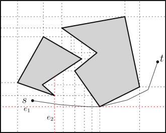
Figure 1: The cell decomposition $\mathcal{D}$ of $\mathcal{P}$, and a shortest path from $s$ to $t$.

Figure 2: Illustrating Lemma 2.1: a shortest path through vertices $v\in V_{\sigma}$ and $v^{\prime}\in V_{\sigma^{\prime}}$.

Lemma 2.1.

Let $\sigma,\sigma^{\prime}$ be any two cells of $\mathcal{D}$. For any point $s\in\sigma$ and any point $t\in\sigma^{\prime}$, if $\sigma$ and $\sigma^{\prime}$ are aligned, then $d(s,t)=|\overline{st}|$; otherwise, there exists an $L_{1}$ shortest path between $s$ and $t$ that passes through two vertices $v\in V_{\sigma}$ and $v^{\prime}\in V_{\sigma^{\prime}}$ (e.g., see Fig. 2).

Proof 2.2.

If two cells $\sigma,\sigma^{\prime}\in\mathcal{D}$ are aligned, then they are contained in a trapezoid $\tau$ of the vertical or horizontal trapezoidal map. Since $\tau$ is convex, any two points in $\tau$ can be joined by a straight segment, so we have $d(s,t)=|\overline{st}|$ for any $s\in\sigma$ and $t\in\sigma$.

Now, suppose that $\sigma$ and $\sigma^{\prime}$ are unaligned (e.g., see Fig. 2). Let $\pi$ be any shortest path between $s$ and $t$. We first observe that $\pi$ intersects one horizontal diagonal $e_{1}$ of $\mathcal{D}$ and one vertical diagonal $e_{2}$, both of which bound $\sigma$ (e.g., see Fig. 2, where $e_{1}$ and $e_{2}$ are highlighted with red color): otherwise, $\sigma$ and $\sigma^{\prime}$ must be aligned. Since $e_{1}$ and $e_{2}$ are bounding $\sigma$, the intersection $v=e_{1}\cap e_{2}$ is a vertex of $\sigma$ (e.g., see Fig. 2). Let $p_{1}$ be the first intersection of $\pi$ with $e_{1}$ while we go along $\pi$ from $s$ to $t$. Similarly, define $p_{2}$ to be the first intersection of $\pi$ with $e_{2}$.

Since $e_{1}$ is horizontal and $e_{2}$ is vertical, the union of the two line segments $\overline{p_{1}v}\cup\overline{vp_{2}}$ is a shortest path between $p_{1}$ and $p_{2}$. We replace the portion of $\pi$ between $p_{1}$ and $p_{2}$ by $\overline{p_{1}v}\cup\overline{vp_{2}}$ to have another $s$-$t$ path $\pi^{\prime}$. Since $\overline{p_{1}v}\cup\overline{vp_{2}}$ is monotone, its length is equal to $|\overline{p_{1}p_{2}}|$ by Fact 1. This implies that $\pi^{\prime}$ is a shortest path between $s$ and $t$ and passes through the vertex $v$.

Symmetrically, the above argument can be applied to the other side, the destination $t$ and the cell $\sigma^{\prime}$, which implies that $\pi^{\prime}$ can be modified to a $s$-$t$ shortest path $\pi^{\prime\prime}$ that passes through $v$ and simultaneously a vertex $v^{\prime}$ of $\sigma^{\prime}$. The lemma thus follows.

2.1 Computing the Geodesic Diameter

In this section, we present an $O(n^{4})$ time algorithm for computing the diameter of $\mathcal{P}$.

The general idea is to consider every pair of cells of $\mathcal{D}$ separately. For each pair of such cells $\sigma,\sigma^{\prime}\in\mathcal{D}$, we compute the maximum geodesic distance between $\sigma$ and $\sigma^{\prime}$, that is, $\max_{s\in\sigma,t\in\sigma^{\prime}}d(s,t)$, called the $(\sigma,\sigma^{\prime})$-constrained diameter. Since $\mathcal{D}$ is a decomposition of $\mathcal{P}$, the diameter of $\mathcal{P}$ is equal to the maximum value of the constrained diameters over all pairs of cells of $\mathcal{D}$. We handle two cases depending on whether $\sigma$ and $\sigma^{\prime}$ are aligned.

If $\sigma$ and $\sigma^{\prime}$ are aligned, by Lemma 2.1, for any $s\in\sigma$ and $t\in\sigma^{\prime}$, we have $d(s,t)=|\overline{st}|$, i.e, the $L_{1}$ distance of $\overline{st}$. Since the $L_{1}$ distance function is convex, the $(\sigma,\sigma^{\prime})$-constrained diameter is always realized by some pair $(v,v^{\prime})$ of two vertices with $v\in V_{\sigma}$ and $v^{\prime}\in V_{\sigma}^{\prime}$. We are thus done by checking at most $16$ pairs of vertices, in $O(1)$ time.

In the following, we assume that $\sigma$ and $\sigma^{\prime}$ are unaligned. Consider any point $s\in\sigma$ and any point $t\in\sigma^{\prime}$. For any vertex $v\in V_{\sigma}$ and any vertex $v^{\prime}\in V_{\sigma^{\prime}}$, consider the path from $s$ to $t$ obtained by concatenating $\overline{sv}$, a shortest path from $v$ to $v^{\prime}$, and $\overline{v^{\prime}t}$, and let $d_{vv^{\prime}}(s,t)$ be its length. Lemma 2.1 ensures that $d(s,t)=\min_{v\in V_{\sigma},v^{\prime}\in V_{\sigma^{\prime}}}d_{vv^{\prime}}(s,t)$. Since $d_{vv^{\prime}}(s,t)=|\overline{sv}|+|\overline{v^{\prime}t}|+d(v,v^{\prime})$ and $d(v,v^{\prime})$ is constant over all $(s,t)\in\sigma\times\sigma^{\prime}$, the function $d_{vv^{\prime}}$ is linear on $\sigma\times\sigma^{\prime}$. Thus, it is easy to compute the $(\sigma,\sigma^{\prime})$-constrained diameter once we know the value of $d(v,v^{\prime})$ for every pair $(v,v^{\prime})$ of vertices.

Lemma 2.3.

For any two cells $\sigma,\sigma^{\prime}\in\mathcal{D}$, the $(\sigma,\sigma^{\prime})$-constrained diameter can be computed in constant time, provided that $d(v,v^{\prime})$ for every pair $(v,v^{\prime})$ with $v\in V_{\sigma}$ and $v^{\prime}\in V_{\sigma^{\prime}}$ has been computed.

Proof 2.4.

The case where $\sigma$ and $\sigma^{\prime}$ are aligned is easy as discussed above. We thus assume they are unaligned.

Assume that we know the value of $d(v,v^{\prime})$ for every pair $(v,v^{\prime})$ with $v\in V_{\sigma}$ and $v^{\prime}\in V_{\sigma^{\prime}}$. Recall that $d(s,t)=\min_{v\in V_{\sigma},v^{\prime}\in V_{\sigma}}d_{vv^{\prime}}(s,t)$ and $d_{vv^{\prime}}(s,t)=|\overline{sv}|+|\overline{v^{\prime}t}|+d(v,v^{\prime})$. Further, note that $|V_{\sigma}|\leq 4,|V_{\sigma^{\prime}}|\leq 4$.

Since each $d_{vv^{\prime}}$ is a linear function on its domain $\sigma\times\sigma^{\prime}$, its graph appears as a hyperplane in a $5$-dimensional space. Thus, the geodesic distance function $d$ restricted on $\sigma\times\sigma^{\prime}$ corresponds to the lower envelope of those hyperplanes. Since there are only a constant number of pairs $(v,v^{\prime})$, the function $d$ can also be explicitly constructed in $O(1)$ time. Finally, we find the highest point on the graph of $d$ by traversing all of its faces.

For each vertex $v$ of $\mathcal{D}$, a straightforward method can compute $d(v,v^{\prime})$ for all other vertices $v^{\prime}$ of $\mathcal{D}$ in $O(n^{2}\log n)$ time, by first computing the shortest path map $S\!P\!M(v)$ [18, 19] in $O(n\log n)$ time and then computing $d(v,v^{\prime})$ for all $v^{\prime}\in\mathcal{D}$ in $O(n^{2}\log n)$ time. We instead give a faster sweeping algorithm in Lemma 2.5 by making use of the property that all vertices on every diagonal of $\mathcal{D}$ are sorted.

Lemma 2.5.

For each vertex $v$ of $\mathcal{D}$, we can evaluate $d(v,v^{\prime})$ for all vertices $v^{\prime}$ of $\mathcal{D}$ in $O(n^{2})$ time.

Proof 2.6.

Our algorithm attains its efficiency by using the property that all vertices on each diagonal of $\mathcal{D}$ are sorted. Specifically, suppose that $\mathcal{D}$ is represented by a standard data structure, e.g., the doubly connected edge list. Then, by traversing each diagonal (either vertical or horizontal), we can obtain a vertically or horizontally sorted list of vertices on that diagonal.

We first compute the shortest path map $S\!P\!M(v)$ in $O(n\log n)$ time [18, 19]. We then apply a standard sweeping technique, say, we sweep $S\!P\!M(v)$ by a vertical line from left to right. The events are when the sweep line hits vertices of $S\!P\!M(v)$, obstacle vertices of $\mathcal{P}$, or vertical diagonals of $\mathcal{D}$. Note that each vertex of $\mathcal{D}$ is either on a vertical diagonal or an obstacle vertex. We use the standard technique to handle the events of vertices of $S\!P\!M(v)$ and $\mathcal{P}$, and each such event costs $O(\log n)$ time. For each event of a vertical diagonal of $\mathcal{D}$, we simply do a linear search on the sweeping status to find the cells of $S\!P\!M(v)$ that contain the cell vertices of $\mathcal{D}$ on the diagonal. Each such event takes $O(n)$ time since each diagonal of $\mathcal{D}$ has $O(n)$ vertices. Note that the total number of events is $O(n)$. Hence, the running time of the sweeping algorithm is $O(n^{2})$.

Thus, after $O(n^{4})$-time preprocessing, for any two cells $\sigma,\sigma^{\prime}\in\mathcal{D}$, the $(\sigma,\sigma^{\prime})$-constrained diameter can be computed in $O(1)$ time by Lemma 2.3. Since $\mathcal{D}$ has $O(n^{2})$ cells, it suffices to handle at most $O(n^{4})$ pairs of cells, resulting in $O(n^{4})$ candidates for the diameter, and the maximum is the diameter. Hence, we obtain the following result.

Theorem 2.7.

The $L_{1}$ geodesic diameter of $\mathcal{P}$ can be computed in $O(n^{4})$ time.

2.2 Computing the Geodesic Center

We now present an algorithm that computes an $L_{1}$ center of $\mathcal{P}$. The observation in Lemma 2.1 plays an important role in our algorithm.

For any point $q\in\mathcal{P}$, we define $R(q)$ to be the maximum geodesic distance between $q$ and any point in $\mathcal{P}$, i.e., $R(q):=\max_{p\in\mathcal{P}}d(p,q)$. A center $q^{*}$ of $\mathcal{P}$ is defined to be a point with $R(q^{*})=\min_{q\in\mathcal{P}}R(q)$. Our approach is again based on the decomposition $\mathcal{D}$: for each cell $\sigma\in\mathcal{D}$, we want to find a point $q\in\sigma$ that minimizes the maximum geodesic distance $d(p,q)$ over all $p\in\mathcal{P}$. We call such a point $q\in\sigma$ a $\sigma$-constrained center. Thus, if $q^{\prime}$ is a $\sigma$-constrained center, then we have $R(q^{\prime})=\min_{q\in\sigma}R(q)$. Clearly, the center $q^{*}$ of $\mathcal{P}$ must be a $\sigma$-constrained center for some $\sigma\in\mathcal{D}$. Our algorithm thus finds a $\sigma$-constrained center for every $\sigma\in\mathcal{D}$, which at last results in $O(n^{2})$ candidates for a center of $\mathcal{P}$.

Consider any cell $\sigma\in\mathcal{D}$. To compute a $\sigma$-constrained center, we investigate the function $R$ restricted to $\sigma$ and exploit Lemma 2.1 again. To utilize Lemma 2.1, for any point $q\in\sigma$, we define $R_{\sigma^{\prime}}(q):=\max_{p\in\sigma^{\prime}}d(p,q)$ for any $\sigma^{\prime}\in\mathcal{D}$. For any $q\in\sigma$, $R(q)=\max_{\sigma^{\prime}\in\mathcal{D}}R_{\sigma^{\prime}}(q)$, that is, $R$ is the upper envelope of all the $R_{\sigma^{\prime}}$ on the domain $\sigma$. Our algorithm explicitly computes the functions $R_{\sigma^{\prime}}$ for all $\sigma^{\prime}\in\mathcal{D}$ and computes the upper envelope $\mathcal{U}$ of the graphs of the $R_{\sigma^{\prime}}$. Then, a $\sigma$-constrained center corresponds to a lowest point on $\mathcal{U}$.

We observe the following for the function $R_{\sigma^{\prime}}$.

Lemma 2.8.

The function $R_{\sigma^{\prime}}$ is piecewise linear on $\sigma$ and has $O(1)$ complexity.

Proof 2.9.

Recall that $R_{\sigma^{\prime}}(q)=\max_{p\in\sigma^{\prime}}d(p,q)$ for $q\in\sigma$. In this proof, we regard $d$ to be restricted on $\sigma\times\sigma^{\prime}\subset\mathbb{R}^{4}$ and use a coordinate system of $\mathbb{R}^{4}$ by introducing $4$ axes, $x$, $y$, $u$, and $w$ with $p=(x,y)\in\sigma$ and $q=(u,w)\in\sigma^{\prime}$. Thus, we may write $R_{\sigma^{\prime}}(q)=R_{\sigma^{\prime}}(x,y)=\max_{(u,w)\in\sigma^{\prime}}d(x,y,u,w)$.

The graph of function $d$ consists of $O(1)$ linear patches as shown in the proof of Lemma 2.3. Once we fully identify the geodesic distance function $d$ on $\sigma\times\sigma^{\prime}$, we consider its graph $S:=\{z=d(x,y,u,w)\}$ for all $(x,y,u,w)\in\sigma\times\sigma^{\prime}$, which is a hypersurface in a $5$-dimensional space $(\sigma\times\sigma^{\prime})\times\mathbb{R}\subset\mathbb{R}^{5}$ with an additional axis $z$. We then project the graph $S$ onto the $(x,y,z)$-space. More precisely, the projection of $S$ is the set $\{(x,y,z)\mid(x,y,u,w,z)\in S\}$. Thus, for any $(x,y)\in\sigma$, $R_{\sigma^{\prime}}(x,y)$ is determined by the highest point in the intersection of the projection with the $z$-axis parallel line through point $(x,y,0)$. This implies that the function $R_{\sigma^{\prime}}$ simply corresponds to the upper envelope (in the $z$-coordinate) of the projection of $S$. Since $S$ consists of $O(1)$ linear patches, so does the upper envelope of its projection, which concludes the proof.

Now, we are ready to describe how to compute a $\sigma$-constrained center. We first handle every cell $\sigma^{\prime}\in\mathcal{D}$ to compute the graph of $R_{\sigma^{\prime}}$ and thus gather its linear patches. Let $\Gamma$ be the family of those linear patches for all $\sigma^{\prime}\in\mathcal{D}$. We then compute the upper envelope of $\Gamma$ and find a lowest point on the upper envelope, which corresponds to a $\sigma$-constrained center. Since $|\Gamma|=O(n^{2})$ by Lemma 2.8, the upper envelope can be computed in $O(n^{4}\alpha(n))$ time by executing the algorithm by Edelsbrunner et al. [12], where $\alpha(\cdot)$ denotes the inverse Ackermann function. The following theorem summarizes our algorithm.

Theorem 2.10.

An $L_{1}$ geodesic center of $\mathcal{P}$ can be computed in $O(n^{6}\alpha(n))$ time.

Proof 2.11.

As a preprocessing, we compute all of the vertex-to-vertex geodesic distances $d(v,v^{\prime})$ for all pairs of vertices of $\mathcal{D}$ in $O(n^{4})$ time. We show that for a fixed $\sigma\in\mathcal{D}$, a $\sigma$-constrained center can be computed in $O(n^{4}\alpha(n))$ time. As discussed in the proof of Lemma 2.3, for any $\sigma^{\prime}\in\mathcal{D}$, the geodesic distance function $d$ restricted on $\sigma\times\sigma^{\prime}$, along with its graph $D$ over $\sigma\times\sigma^{\prime}$, can be specified in $O(1)$ time. By Lemma 2.8, from $D$ we can describe the function $R_{\sigma^{\prime}}$ in $O(1)$ time. The last task is to compute the upper envelope of all $R_{\sigma^{\prime}}$ in $O(n^{4}\alpha(n))$ time, as discussed above, by executing the algorithm by Edelsbrunner et al. [12].

3 Exploiting the Extended Corridor Structure

In this section, we briefly review the extended corridor structure of $\mathcal{P}$ and present new observations, which will be crucial for our improved algorithms in Section 4. The corridor structure has been used for solving shortest path problems [9, 16, 17]. Later some new concepts such as “bays,” “canals,” and the “ocean” were introduced [10, 11], referred to as the “extended corridor structure.”

3.1 The Extended Corridor Structure

Let $\mathcal{T}$ denote an arbitrary triangulation of $\mathcal{P}$ (e.g., see Figure 4). We can obtain $\mathcal{T}$ in $O(n\log n)$ time or $O(n+h\log^{1+\epsilon}h)$ time for any $\epsilon>0$ [7]. Let $G$ denote the dual graph of $\mathcal{T}$, i.e., each node of $G(\mathcal{P})$ corresponds to a triangle in $\mathcal{T}(\mathcal{P})$ and each edge connects two nodes of $G(\mathcal{P})$ corresponding to two triangles sharing a diagonal of $\mathcal{T}(\mathcal{P})$. Based on $G$, one can obtain a planar $3$-regular graph, possibly with loops and multi-edges, by repeatedly removing all degree-one nodes and then contracting all degree-two nodes. The resulting $3$-regular graph has $O(h)$ faces, nodes, and edges [17]. Each node of the graph corresponds to a triangle in $\mathcal{T}$, called a junction triangle. The removal of all junction triangles from $\mathcal{P}$ results in $O(h)$ components, called corridors, each of which corresponds to an edge of the graph. See Figure 4. Refer to [17] for more details.

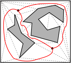
Figure 3: A triangulation $\mathcal{T}$ of $\mathcal{P}$ and the $3$-regular graph obtained from the dual graph of $\mathcal{T}$ whose nodes and edges are depicted by black dots and red solid curves. Each junction triangle corresponds to a node and removing all junction triangles results in three corridors, in this figure, each of which corresponds to an edge of the graph.

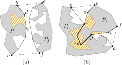
Figure 4: Hourglasses $H_{K}$ in corridors $K$. The dashed segments $\overline{be}$ and $\overline{af}$ are diagonals of junction triangles in $\mathcal{T}$. (a) $H_{K}$ is open. Five bays can be seen. A bay with gate $\overline{cd}$ is shown as the shaded region. (b) $H_{K}$ is closed. There are three bays and a canal, and the shaded region depicts the canal with two gates $\overline{dx}$ and $\overline{cy}$.

Next we briefly review the concepts of bays, canals, and the ocean. Refer to [10, 11] for more details.

Let $P_{1},\ldots,P_{h}$ be the $h$ holes of $\mathcal{P}$ and $P_{0}$ be the outer polygon of $\mathcal{P}$. For simplicity, a hole may also refer to the unbounded region outside $P_{0}$ hereafter. The boundary $\partial K$ of a corridor $K$ consists of two diagonals of $\mathcal{T}$ and two paths along the boundary of holes $P_{i}$ and $P_{j}$, respectively (it is possible that $P_{i}$ and $P_{j}$ are the same hole, in which case one may consider $P_{i}$ and $P_{j}$ as the above two paths respectively). Let $a,b\in P_{i}$ and $e,f\in P_{j}$ be the endpoints of the two paths, respectively, such that $\overline{be}$ and $\overline{fa}$ are diagonals of $\mathcal{T}$, each of which bounds a junction triangle. See Figure 4. Let $\pi_{ab}$ (resp., $\pi_{ef}$) denote the Euclidean shortest path from $a$ to $b$ (resp., $e$ to $f$) inside $K$. The region $H_{K}$ bounded by $\pi_{ab},\pi_{ef}$, $\overline{be}$, and $\overline{fa}$ is called an hourglass, which is either open if $\pi_{ab}\cap\pi_{ef}=\emptyset$, or closed, otherwise. If $H_{K}$ is open, then both $\pi_{ab}$ and $\pi_{ef}$ are convex chains and are called the sides of $H_{K}$; otherwise, $H_{K}$ consists of two “funnels” and a path $\pi_{K}=\pi_{ab}\cap\pi_{ef}$ joining the two apices of the two funnels, called the corridor path of $K$. The two funnel apices (e.g., $x$ and $y$ in Figure 4(b)) connected by $\pi_{K}$ are called the corridor path terminals. Note that each funnel comprises two convex chains.

We consider the region of $K$ minus the interior of $H_{K}$, which consists of a number of simple polygons facing (i.e., sharing an edge with) one or both of $P_{i}$ and $P_{j}$. We call each of these simple polygons a bay if it is facing a single hole, or a canal if facing both holes. Each bay is bounded by a portion of the boundary of a hole and a segment $\overline{cd}$ between two obstacle vertices $c,d$ that are consecutive along a side of $H_{K}$. We call the segment $\overline{cd}$ the gate of the bay. (See Figure 4(a).) On the other hand, there exists a unique canal for each corridor $K$ only when $H_{K}$ is closed and the two holes $P_{i}$ and $P_{j}$ both bound the canal. The canal in $K$ in this case completely contains the corridor path $\pi_{K}$. A canal has two gates $\overline{xd}$ and $\overline{yc}$ that are two segments facing the two funnels, respectively, where $x,y$ are the corridor path terminals and $d,c$ are vertices of the funnels. (See Figure 4(b).) Note that each bay or canal is a simple polygon.

Let $\mathcal{M}\subseteq\mathcal{P}$ be the union of all junction triangles, open hourglasses, and funnels. We call $\mathcal{M}$ the ocean. Its boundary $\partial\mathcal{M}$ consists of $O(h)$ convex vertices and $O(h)$ reflex chains each of which is a side of an open hourglass or of a funnel. Note that $\mathcal{P}\setminus\mathcal{M}$ consists of all bays and canals of $\mathcal{P}$.

For convenience of discussion, define each bay/canal in such a way that they do not contain their gates and hence their gates are contained in $\mathcal{M}$; therefore, each point of $\mathcal{P}$ is either in a bay/canal or in $\mathcal{M}$, but not in both. After the triangulation $\mathcal{T}$ is obtained, computing the ocean, all bays and canals can be done in $O(n)$ time [10, 11, 17].

Roughly speaking, the reason we partition $\mathcal{P}$ into the ocean, bays, and canals is to facilitate evaluating the distance $d(s,t)$ for any two points $s$ and $t$ in $\mathcal{P}$. For example, if both $s$ and $t$ are in $\mathcal{M}$, then we can use a similar method as in Section 2 to evaluate $d(s,t)$. However, the challenging case happens when one of $s$ and $t$ is in $\mathcal{M}$ and the other is in a bay or canal.

The following lemma is one of our key observations for our improved algorithms in Section 4. It essentially tells that for any point $s\in\mathcal{P}$ and any bay or canal $A$, the farthest point of $s$ in $A$ is achieved on the boundary $\partial A$, which is similar in spirit to the simple polygon case.

Lemma 3.1.

Let $s\in\mathcal{P}$ be any point and $A$ be a bay or canal of $\mathcal{P}$. Then, for any $t\in A$, there exists $t^{\prime}\in\partial A$ such that $d(s,t)\leq d(s,t^{\prime})$. Equivalently, $\max_{t\in A}d(s,t)=\max_{t\in\partial A}d(s,t)$.

Proof 3.2.

Recall that the gates of $A$ are not contained in $A$ but in the ocean $\mathcal{M}$. Let $\bar{A}$ be the closure of $A$, that is, $\bar{A}$ consists of $A$ and its gates. For any $p,q\in\bar{A}$, let $d_{A}(p,q)$ be the $L_{1}$ geodesic distance in $\bar{A}$. Since $\bar{A}$ is a simple polygon, Fact 2 implies that there is a unique Euclidean shortest path $\pi_{2}(p,q)$ in $\bar{A}$ between any $p,q\in\bar{A}$, and $d_{A}(p,q)=|\pi_{2}(p,q)|$. In general, we have $d_{A}(p,q)\geq d(p,q)$.

Depending on whether $A$ is a bay or a canal, our proof will consider two cases. We first prove a basic property as follows.

A Basic Property

Consider any point $s^{\prime}\in\mathcal{P}$ and any point $t^{\prime}\in A$. Then, we claim that there exists a shortest $s^{\prime}$-$t^{\prime}$ path $\pi$ with the following property (*):

(*) $\pi$ crosses each gate of $A$ at most once and each component of $\pi\cap\bar{A}$ is the unique Euclidean shortest path $\pi_{2}(p,q)$ for some points $p,q\in\bar{A}$.

Consider any shortest $s^{\prime}$-$t^{\prime}$ path $\pi^{\prime}$. If $\pi^{\prime}$ crosses a gate $g$ of $A$ at least twice, then let $p\in g$ and $q\in g$ be the first and last points on $g$ we encounter when walking along $\pi^{\prime}$ from $s^{\prime}$ to $t^{\prime}$. We can replace the portion of $\pi^{\prime}$ between $p$ and $q$ with the line segment $\overline{pq}$ by Fact 1 to obtain another shortest path that crosses $g$ at most once. One can repeat this procedure for all gates of $A$ to have a shortest path $\pi^{\prime\prime}$ crossing each gate of $A$ at most once. Then, we take a connected component of $\pi^{\prime\prime}\cap\bar{A}$, which is an $L_{1}$ shortest path between its two endpoints $p,q$ inside $\bar{A}$. This implies that $d(p,q)=d_{A}(p,q)=|\pi_{2}(p,q)|$, so we can replace the component by $\pi_{2}(p,q)$. Repeat this for all components of $\pi^{\prime\prime}\cap\bar{A}$ to obtain another shortest $s^{\prime}$-$t^{\prime}$ path $\pi$ with the desired property (*).

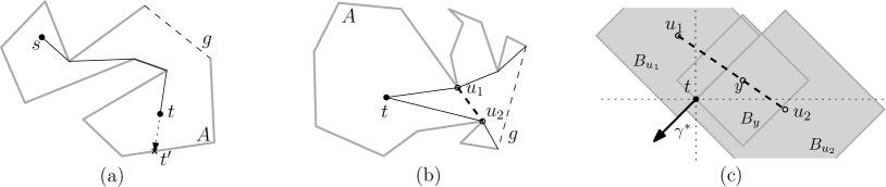
Figure 5: Illustration to the proof of Lemma 3.1 when $A$ is a bay. (a) When $s\in\bar{A}$ and (b)(c) when $s\notin\bar{A}$.

The Bay Case

To prove the lemma, we first prove the case where $A$ is a bay. Then, $A$ has a unique gate $g$. Recall that the gate $g$ is not contained in $A$. Depending on whether $s$ is in $\bar{A}$, there are two cases.

• Suppose that $s\in\bar{A}$. Let $t\in A$ be any point in $A$. By our claim, there exists a shortest $s$-$t$ path $\pi$ in $\mathcal{P}$ with property (*). Since both $s$ and $t$ lie in $\bar{A}$, $\pi$ does not cross $g$, and is thus contained in $\bar{A}$. Moreover, by property (*), we have $\pi=\pi_{2}(s,t)$. Hence, $d(s,t)=d_{A}(s,t)$.

  If $t$ lies on $\partial A$, then the lemma trivially holds. Suppose that $t$ lies in the interior of $A$. Then, we can extend the last segment of $\pi_{2}(s,t)$ until it hits a point $t^{\prime}$ on the boundary $\partial A$. See Figure 5(a). Again since $\bar{A}$ is a simple polygon, the extended path is indeed $\pi_{2}(s,t^{\prime})$. By the above argument, $d(s,t^{\prime})=d_{A}(s,t^{\prime})=|\pi_{2}(s,t^{\prime})|$, which is strictly larger than $|\pi_{2}(s,t)|=d(s,t)$.

• Suppose that $s\notin\bar{A}$. Then, any shortest path from $s$ to any point $t\in A$ must cross the gate $g$. This implies that $d(s,t)=\min_{x\in g}\{d(s,x)+d_{A}(x,t)\}$ for any $t\in A$. We show that there exists $t^{\prime}\in\partial A$ such that for any point $x\in g$, it holds that $d_{A}(x,t)\leq d_{A}(x,t^{\prime})$, which implies that $d(s,t)=\min_{x\in g}\{d(s,x)+d_{A}(x,t)\}\leq\min_{x\in g}\{d(s,x)+d_{A}(x,t^{\prime})\}=d(s,t^{\prime})$. For the purpose, we consider the union of $\pi_{2}(x,t)$ for all $x\in g$. The union forms a funnel $F_{g}(t)$ plus the Euclidean shortest path $\pi_{2}(u,t)$ from the apex $u$ of $F_{g}(t)$ to $t$. If $u\neq t$, then we extend the last segment of $\pi_{2}(u,t)$ to a point $t^{\prime}$ on the boundary $\partial A$, similarly to the previous case so that $d_{A}(u,t)\leq d_{A}(u,t^{\prime})$ and thus $d_{A}(x,t)\leq d_{A}(x,t^{\prime})$ for any $x\in g$. Otherwise, if $u=t$, then let $u_{1}$ and $u_{2}$ be the two vertices of $F_{g}(t)$ adjacent to the apex $t$. See Figure 5(b).

  Observe that the segment $\overline{u_{1}u_{2}}$ separates $t$ and the gate $g$, and hence path $\pi_{2}(x,t)$ for any $x\in g$ crosses $\overline{u_{1}u_{2}}$. We now claim that there exists a ray $\gamma^{*}$ from $t$ such that as $t$ moves along $\gamma^{*}$, $d_{A}(t,y)$ for any fixed $y\in\overline{u_{1}u_{2}}$ is nondecreasing. If the claim is true, then we select $t^{\prime}=\gamma^{*}\cap\partial A$, so the lemma follows since it holds that $d_{A}(t,x)=\min_{y_{\in}\overline{u_{1}u_{2}}}\{d_{A}(t,y)+d_{A}(y,x)\}$ $\leq\min_{y_{\in}\overline{u_{1}u_{2}}}\{d_{A}(t^{\prime},y)+d_{A}(y,x)\}=d_{A}(t^{\prime},x)$ for any $x\in g$. Next, we prove the claim.

  For each $y\in\overline{u_{1}u_{2}}$, let $B_{y}$ be the $L_{1}$ disk centered at $y$ with radius $d_{A}(y,t)=|\overline{yt}|$. See Figure 5(c). Since $t$ lies on the boundary of $B_{y}$, as we move $t$ along a ray $\gamma$ in some direction outwards $B_{y}$, $|\overline{yt}|$ is not decreasing, that is, for any $p\in\gamma$, $|\overline{yp}|\geq|\overline{yt}|$. This also implies that $d_{A}(y,p)\geq|\overline{yp}|\geq|\overline{yt}|=d_{A}(y,t)$. Let $h_{y}$ be the set of all such rays $\gamma$ that as $t$ moves along $\gamma$, $|\overline{yt}|$ is not decreasing. Our goal is thus to show that $\bigcap_{y\in\overline{u_{1}u_{2}}}h_{y}\neq\emptyset$, and pick $\gamma^{*}$ as any ray in the intersection. For the purpose, we consider the four quadrants—left-upper, right-upper, left-lower, and right-lower—centered at $t$. Then, since the $B_{y}$ are all $L_{1}$ disks, the set $h_{y}$ only depends on which quadrant $y$ belongs to; more precisely, for any $y$ in a common quadrant, the set $h_{y}$ stays constant. For example, for any $y\in\overline{u_{1}u_{2}}$ lying in the right-upper quadrant, then $h_{y}$ is commonly the set of all rays from $t$ in direction between $135^{\circ}$ and $315^{\circ}$, inclusively, since $t$ lies on the bottom-left edge of $B_{y}$ in this case. Thus, the directions of all rays in $h_{y}$ span an angle of exactly $180^{\circ}$. Moreover, $\overline{u_{1}u_{2}}$ is a line segment and thus intersects only three quadrants. Therefore, $\bigcap_{y\in\overline{u_{1}u_{2}}}h_{y}$ is equal to the intersection of at most three different sets of rays, whose directions span an angle of $180^{\circ}$. (Figure 5(c) illustrates an example scene when $\overline{u_{1}u_{2}}$ intersects three quadrants centered at $t$.) This implies that $\bigcap_{y\in\overline{u_{1}u_{2}}}h_{y}\neq\emptyset$.

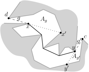
Figure 6: Illustration to the proof of Lemma 3.1 when $A$ is a canal with two gates $g=\overline{dx}$ and $g^{\prime}=\overline{cy}$.

The Canal Case

Above, we have proved the lemma for the bay case where $A$ is a bay. Next, we turn to the canal case: suppose that $A$ is a canal.

Let $g=\overline{dx}$ and $g^{\prime}=\overline{cy}$ be the two gates of $A$, where $x$ and $y$ are the two corridor path terminals (e.g., see Figure 6). We extend $g$ from $x$ into the interior of $A$, in the direction opposite to $d$. Note that due to the definition of canals, this extension always goes into the interior of $A$ (refer to [10] for detailed discussion). Let $x^{\prime}$ be the first point on $\partial A$ hit by the extension. The line segment $\overline{xx^{\prime}}$ partitions $A$ into two simple polygons, and the one containing $d$ is denoted by $A_{g}$. We consider $\overline{dx^{\prime}}$ as an edge of $A_{g}$, but for convenience of discussion, we assume that $A_{g}$ does not contain the segment $\overline{dx^{\prime}}$. Define $A_{g^{\prime}}$ analogously for the other gate $g^{\prime}=\overline{cy}$. If $t\in A_{g}$, then we can view $A_{g}$ as a “bay” with gate $\overline{dx^{\prime}}$, and apply the identical argument as done in the bay case, concluding that for any $t\in A_{g}$ there exists $t^{\prime}\in\partial A_{g}$ such that $d(s,t)\leq d(s,t^{\prime})$. If $t^{\prime}\in\partial A$, then we are done. Otherwise, if $t^{\prime}\in\overline{xx^{\prime}}$, then $s\in A_{g}$ according to our analysis on the bay case. In this case, we move $t^{\prime}$ along $\overline{xx^{\prime}}$ to $x$ or $x^{\prime}$, since $\max\{d(s,x),d(s,x^{\prime})\}\geq d(s,t^{\prime})\geq d(s,t)$, we are done. The case of $t\in A_{g^{\prime}}$ is analogous.

Let $\widehat{A}:=A\setminus(A_{g}\cup A_{g^{\prime}})$. From now on, we suppose $t\in\widehat{A}$. Observe that for any $p\in g$, $\pi_{2}(p,t)$ passes through the corridor path terminal $x$ since $t\notin A_{g}$ [10]; symmetrically, for any $p^{\prime}\in g^{\prime}$, $\pi_{2}(p^{\prime},t)$ passes through $y$. Consider any $L_{1}$ shortest $s$-$t$ path $\pi$ in $\mathcal{P}$ with property (*). We classify $\pi$ into one of the following three types: (a) $\pi$ lies inside $A$, that is, $\pi=\pi_{2}(s,t)$, (b) when walking along $\pi$ from $s$ to $t$, the last gate crossed by $\pi$ is $g$, or (c) is $g^{\prime}$. Note that $\pi$ falls into one of the three cases. In case (a), indeed we have $s\in A$ and $d(s,t)=d_{A}(s,t)$. In case (b), $\pi$ consists of a shortest path from $s$ to $x$ and $\pi_{2}(x,t)$, and thus $d(s,t)=d(s,x)+d_{A}(x,t)$. Symmetrically, in case (c), we have $d(s,t)=d(s,y)+d_{A}(y,t)$.

Depending on whether $s\in\bar{A}$ or not, we handle two possibilities. In the following, we assume property (*) when we discuss any shortest $s$-$t$ path.

• Suppose that $s\notin\bar{A}$. Then, any shortest $s$-$t$ path in $\mathcal{P}$ must cross a gate of $A$. This means that there is no shortest $s$-$t$ path of type (a), and we have $d(s,t)=\min\{d(s,x)+d_{A}(x,t),d(s,y)+d_{A}(y,t)\}$. Consider a decomposition of $\widehat{A}$ into three regions $R_{x}$, $R_{y}$, and $B$ such that $R_{x}=\{p\in\widehat{A}\mid d(s,x)+d_{A}(x,p)<d(s,y)+d_{A}(y,p)\}$, $R_{y}=\{p\in\widehat{A}\mid d(s,x)+d_{A}(x,p)>d(s,y)+d_{A}(y,p)\}$, and $B=\{p\in\widehat{A}\mid d(s,x)+d_{A}(x,p)=d(s,y)+d_{A}(y,p)\}$. This decomposition is clearly the geodesic Voronoi diagram in simple polygon $\widehat{A}$ of two sites $\{x,y\}$ with additive weights. See Aronov [2] and Papadopoulou and Lee [20]. Also, we have that $d(s,t)=d(s,x)+d_{A}(x,t)$ for any $t\in R_{x}$; $d(s,t)=d(s,y)+d_{A}(y,t)$ for any $t\in R_{y}$. The region $B$ is called the bisector between $x$ and $y$. By the property of Voronoi diagrams [2, 20], $B=\partial R_{x}\cap\partial R_{y}$ and $B$ is a path connecting two points on $\partial\widehat{A}$. Let $b_{0}\in B$ be the intersection $\pi_{2}(x,y)\cap B$. Then, $d_{A}(x,b_{0})=d_{A}(y,b_{0})\leq d_{A}(x,b)=d_{A}(y,b)$ for any $b\in B$, and moreover if we move $b$ along $B$ in one direction from $b_{0}$, $d_{A}(x,b)$ is nondecreasing. Thus, $\max_{b\in B}d_{A}(x,b)$ is attained when $b$ is an endpoint of $B$.

  When $t\in\partial A$, the lemma is trivial. If $t\in B$, then we let $t^{\prime}$ be the endpoint of $B$ in direction away from $b_{0}$. Then, by the property of the bisector $B$, we have $d_{A}(x,t)\leq d_{A}(x,t^{\prime})$ and $d_{A}(y,t)\leq d_{A}(y,t^{\prime})$, and hence $d(s,t)\leq d(s,t^{\prime})$. If $t^{\prime}$ lies on the boundary $\partial A$, we conclude the lemma; otherwise, $t^{\prime}$ may lie on $\partial\widehat{A}\setminus\partial A$, say on $\overline{xx^{\prime}}$. In this case, we apply the analysis of the bay case where $s\notin A_{g}$ to find a point $t^{\prime\prime}$ on $\partial A$ such that $d(s,t^{\prime})\leq d(s,t^{\prime\prime})$.

  If $t$ lies in the interior of $R_{x}$, then we extend the last segment of $\pi_{2}(x,t)$ until it hits a point $t^{\prime}$ on $\partial R_{x}$. Then, we have that $d(s,t^{\prime})\geq d(s,t)$. Note that $t^{\prime}$ lies on $\partial\widehat{A}$ or on $B$; in any case, we apply the above argument so that we can find a point $t^{\prime\prime}$ on $\partial A$ with $d(s,t^{\prime\prime})\geq d(s,t^{\prime})\geq d(s,t)$. The case where $t$ lies in the interior of $R_{y}$ is handled analogously.

• Finally, suppose that $s\in\bar{A}$. We again consider the $L_{1}$ geodesic Voronoi diagram in $\widehat{A}$ of three sites $\{s,x,y\}$ with additive weights $0,d(s,x),d(s,y)$, respectively. As done above, we observe that the maximum value $\max_{t\in\widehat{A}}d(s,t)$ is attained when $t\in\partial A$ or $t$ is a Voronoi vertex. The former case is analyzed above. Here, we prove that the latter case cannot happen. Note that there are three shortest paths of different types between $s$ and the Voronoi vertex while there are exactly two shortest paths of types (b) and (c) to any point on the bisector between $x$ and $y$. In the following, we show that the bisector between $x$ and $y$ cannot appear in the Voronoi diagram, which implies that the Voronoi diagram has no vertex.

  

  Figure 7: Illustration to the proof of Lemma 3.1 when $A$ is a canal.

  

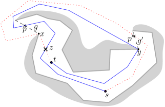
  Figure 8: Illustrating two shortest $s$-$t$ paths $\pi$ (red dotted) and $\pi^{\prime}$ (blue solid), intersecting at $z$, in a canal with two gates $g$ and $g^{\prime}$.

  Suppose to the contrary that the bisector between $x$ and $y$ appears as a nonempty Voronoi edge of the Voronoi diagram, and that $t$ is a point on it. That is, $d(s,t)=d(s,x)+d_{A}(x,t)=d(s,y)+d_{A}(y,t)>d_{A}(s,t)$. Let $\pi$ and $\pi^{\prime}$ be two shortest $s$-$t$ paths of type (b) and (c), respectively. Thus, $\pi$ passes through $x$ and $\pi^{\prime}$ passes through $y$ to reach $t\in\widehat{A}$. By property (*), $\pi$ crosses $g^{\prime}$ first and then $g$ when walking along $\pi$ from $s$ to $t$, and $\pi^{\prime}$ crosses $g$ first and then $g^{\prime}$. Let $p\in g$ and $p^{\prime}\in g^{\prime}$ be the last point of $\pi^{\prime}\cap g$ and $\pi\cap g^{\prime}$, respectively, when we walk along $\pi$ and $\pi^{\prime}$ from $s$ to $t$.

  We claim that $\pi$ and $\pi^{\prime}$ intersect each other in a point other than $s$ and $t$. Indeed, consider the loop $L$ formed by the subpath of $\pi$ between $s$ and $x$, the segment $\overline{xp}$, and the subpath of $\pi^{\prime}$ between $s$ and $p$. See Figure 8. Also, let $U$ be a disk centered at $p$ with arbitrarily small radius and $q\in\pi^{\prime}\cap\partial U$ be the point on $\pi^{\prime}$ not lying in $A$. If the loop $L$ does not separate $q$ and $t$, then the subpath of $\pi$ from $x$ to $t$ must intersect $\pi^{\prime}$ in a point other than $t$ (see Fig. 8), and thus the claim follows; otherwise, the subpath of $\pi^{\prime}$ from $q$ to $t$ must cross $L$ at some point other than $s$ and $t$, and thus the claim also follows.

  Let $z\in\pi\cap\pi^{\prime}\setminus\{s,t\}$ (see Fig. 8), and $\pi_{zt}$ and $\pi^{\prime}_{zt}$ be the subpath of $\pi$ and $\pi^{\prime}$, respectively, from $z$ to $t$. By the property of shortest paths, we have $|\pi_{zt}|=|\pi^{\prime}_{zt}|=d(z,t)$. Hence, replacing $\pi_{zt}$ by $\pi^{\prime}_{zt}$ in $\pi$ results in another shortest $s$-$t$ path $\pi^{\prime\prime}$. If $\pi^{\prime\prime}$ lies inside $\bar{A}$, then we have $d(s,t)=|\pi^{\prime\prime}|\geq d_{A}(s,t)$. Otherwise, $\pi^{\prime\prime}$ crosses $g^{\prime}$ twice at $p^{\prime}$ and $y$, and thus replacing the subpath of $\pi^{\prime\prime}$ from $p^{\prime}$ to $y$ by $\overline{p^{\prime}y}$ results in another shortest path inside $\bar{A}$. In either way, there is another $L_{1}$ shortest $s$-$t$ path of type (a), and hence $d(s,t)=d_{A}(s,t)$, a contradiction to the assumption that $t$ lies on the bisector between $x$ and $y$.

This finishes the proof of the lemma.

3.2 Shortest Paths in the Ocean $\mathcal{M}$

We now discuss shortest paths in the ocean $\mathcal{M}$. Recall that corridor paths are contained in canals, but their terminals are on $\partial\mathcal{M}$. By using the corridor paths and $\mathcal{M}$, finding an $L_{1}$ or Euclidean shortest path between two points $s$ and $t$ in $\mathcal{M}$ can be reduced to the convex case since $\partial\mathcal{M}$ consists of $O(h)$ convex chains. For example, suppose both $s$ and $t$ are in $\mathcal{M}$. Then, there must be a shortest $s$-$t$ path $\pi$ that lies in the union of $\mathcal{M}$ and all corridor paths [9, 11, 17].

Consider any two points $s$ and $t$ in $\mathcal{M}$. A shortest $s$-$t$ path $\pi(s,t)$ in $\mathcal{P}$ is a shortest path in $\mathcal{M}$ that possibly contains some corridor paths. Intuitively, one may view corridor paths as “shortcuts” among the components of the space $\mathcal{M}$. As in [17], since $\partial\mathcal{M}$ consists of $O(h)$ convex vertices and $O(h)$ reflex chains, the complementary region $\mathcal{P}^{\prime}\setminus\mathcal{M}$ (where $\mathcal{P}^{\prime}$ refers to the union of $\mathcal{P}$ and all its holes) can be partitioned into a set $\mathcal{B}$ of $O(h)$ convex objects with a total of $O(n)$ vertices (e.g., by extending an angle-bisecting segment inward from each convex vertex [17]). If we view the objects in $\mathcal{B}$ as obstacles, then $\pi$ is a shortest path avoiding all obstacles of $\mathcal{B}$ but possibly containing some corridor paths. Note that our algorithms can work on $\mathcal{P}$ and $\mathcal{M}$ directly without using $\mathcal{B}$; but for ease of exposition, we will discuss our algorithm with the help of $\mathcal{B}$.

Each convex obstacle $Q$ of $\mathcal{B}$ has at most four extreme vertices: the topmost, bottommost, leftmost, and rightmost vertices, and there may be some corridor path terminals on the boundary of $Q$. We connect the extreme vertices and the corridor path terminals on $\partial Q$ consecutively by line segments to obtain another polygon, denoted by $core(Q)$ and called the core of $Q$ (see Figure 10). Let $\mathcal{P}_{core}$ denote the complement of the union of all cores $core(Q)$ for all $Q\in\mathcal{B}$ and corridor paths in $\mathcal{P}$. Note that the number of vertices of $\mathcal{P}_{core}$ is $O(h)$ and $\mathcal{M}\subseteq\mathcal{P}_{core}$. For $s,t\in\mathcal{P}_{core}$, let $d_{core}(s,t)$ be the geodesic distance between $s$ and $t$ in $\mathcal{P}_{core}$.

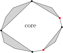
Figure 9: Illustrating the core of a convex obstacle: the (red) squared vertices are corridor path terminals.

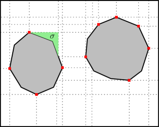
Figure 10: Illustrating the core-based cell decomposition $\mathcal{D}_{\!\mathcal{M}}$: the (red) squared vertices are core vertices and the green cell $\sigma$ is a boundary cell.

The core structure leads to a more efficient way to find an $L_{1}$ shortest path between two points in $\mathcal{P}$. Chen and Wang [9] proved that an $L_{1}$ shortest path between $s,t\in\mathcal{M}$ in $\mathcal{P}_{core}$ can be locally modified to an $L_{1}$ shortest path in $\mathcal{P}$ without increasing its $L_{1}$ length.

Lemma 3.3 ([9]).

For any two points $s$ and $t$ in $\mathcal{M}$, $d(s,t)=d_{core}(s,t)$ holds.

Hence, to compute $d(s,t)$ between two points $s$ and $t$ in $\mathcal{M}$, it is sufficient to consider only the cores and the corridor paths, that is, $\mathcal{P}_{core}$. We thus reduce the problem size from $O(n)$ to $O(h)$. Let $S\!P\!M_{core}(s)$ be a shortest path map for any source point $s\in\mathcal{M}$. Then, $S\!P\!M_{core}(s)$ has $O(h)$ complexity and can be computed in $O(h\log h)$ time [9].

3.3 Decomposition of the Ocean $\mathcal{M}$

We introduce a core-based cell decomposition $\mathcal{D}_{\!\mathcal{M}}$ of the ocean $\mathcal{M}$ (see Figure 10) in order to fully exploit the advantage of the core structure in designing algorithms computing the $L_{1}$ geodesic diameter and center. For any $Q\in\mathcal{B}$, the vertices of $core(Q)$ are called core vertices.

The construction of $\mathcal{D}_{\!\mathcal{M}}$ is analogous to that of the previous cell decomposition $\mathcal{D}$ for $\mathcal{P}$. We first extend a horizontal line only from each core vertex until it hits $\partial\mathcal{M}$ to have a horizontal diagonal, and then extend a vertical line from each core vertex and each endpoint of the above horizontal diagonal. The resulting cell decomposition induced by the above diagonals is $\mathcal{D}_{\!\mathcal{M}}$. Hence, $\mathcal{D}_{\!\mathcal{M}}$ is constructed in $\mathcal{M}$ with respect to core vertices. Note that $\mathcal{D}_{\!\mathcal{M}}$ consists of $O(h^{2})$ cells and can be built in $O(n\log n+h^{2})$ time by a typical plane sweep algorithm. We call a cell $\sigma$ of $\mathcal{D}_{\!\mathcal{M}}$ a boundary cell if $\partial\sigma\cap\partial\mathcal{M}\neq\emptyset$. For any boundary cell $\sigma$, the portion $\partial\sigma\cap\partial\mathcal{M}$ appears as a convex chain of $Q\in\mathcal{B}$ by our construction of its core and $\mathcal{D}_{\mathcal{M}}$; since $\partial\sigma\cap\partial\mathcal{M}$ may contain multiple vertices of $\mathcal{M}$, the complexity of $\sigma$ may not be constant. Any non-boundary cell of $\mathcal{D}_{\!\mathcal{M}}$ is a rectangle bounded by four diagonals. Each vertex of $\mathcal{D}_{\!\mathcal{M}}$ is either an endpoint of its diagonal or an intersection of two diagonals; thus, the number of vertices of $\mathcal{D}_{\!\mathcal{M}}$ is $O(h^{2})$.

Below we prove an analogue of Lemma 2.1 for the decomposition $\mathcal{D}_{\!\mathcal{M}}$ of $\mathcal{M}$. Let $V_{\sigma}$ be the set of vertices of $\mathcal{D}_{\!\mathcal{M}}$ incident to $\sigma$. Note that $|V_{\sigma}|\leq 4$. We define the alignedness relation between two cells of $\mathcal{D}_{\!\mathcal{M}}$ analogously to that for $\mathcal{D}$. We then observe an analogy to Lemma 2.1.

Lemma 3.4.

Let $\sigma,\sigma^{\prime}$ be any two cells of $\mathcal{D}_{\!\mathcal{M}}$. If they are aligned, then $d(s,t)=|\overline{st}|$ for any $s\in\sigma$ and $t\in\sigma^{\prime}$; otherwise, there exists a shortest $s$-$t$ path in $\mathcal{P}$ containing two vertices $v\in V_{\sigma}$ and $v^{\prime}\in V_{\sigma^{\prime}}$ with $d(s,t)=|\overline{sv}|+d(v,v^{\prime})+|\overline{v^{\prime}t}|$.

Proof 3.5.

We first discuss the case where $\sigma$ and $\sigma^{\prime}$ are aligned. In this case, they are bounded by two consecutive parallel diagonals of $\mathcal{D}_{\!\mathcal{M}}$, and let $S\subset\mathcal{M}$ be the region in between the two diagonals. Since $S$ consists of two monotone concave chains and the two diagonals by our construction of $\mathcal{D}_{\!\mathcal{M}}$, it is not difficult to see that any $s\in\sigma$ and $t\in\sigma^{\prime}$ can be joined by a monotone path $\pi$ inside $S$. This implies that $|\pi|=|\overline{st}|=d(s,t)$ by Fact 1.

Next, we consider the unaligned case. Suppose that $\sigma$ and $\sigma^{\prime}$ are unaligned. By Lemma 3.3, there exists a shortest $s$-$t$ path $\pi$ in $\mathcal{P}$ such that $\pi$ lies inside the union $\mathcal{M}$ and all the corridor paths of $\mathcal{P}$. Our proof for this case is analogous to that of Lemma 2.1. Since $\sigma$ and $\sigma^{\prime}$ are unaligned, there are two possibilities when we walk along $\pi$ from $s$ to $t$: either we meet a horizontal diagonal $e_{1}$ and a vertical diagonal $e_{2}$ of $\mathcal{D}_{\!\mathcal{M}}$ that bound $\sigma$, or enter a corridor path via its terminal $x$. In the former case, we can apply the same argument as done in the proof of Lemma 2.1 to show that $\pi$ can be modified to pass through a vertex $v\in V_{\sigma}$ with $v=e_{1}\cap e_{2}$ without increasing the length of the resulting path. In the latter case, observe by our construction of $\mathcal{D}_{\!\mathcal{M}}$ that $x$ is also a vertex of $\mathcal{D}_{\!\mathcal{M}}$ and there is a diagonal extended from $x$. If $x\in V_{\sigma}$, we are done since $d(s,x)=|\overline{sx}|$ as discussed above (any cell $\sigma$ is aligned with itself). Otherwise, there is a unique cell $\sigma^{\prime\prime}\neq\sigma\in\mathcal{D}_{\!\mathcal{M}}$ with $x\in V_{\sigma^{\prime\prime}}$ that is aligned with $\sigma$, and there is a common diagonal $e$ bounding $\sigma$ and $\sigma^{\prime\prime}$. In this case, since $\pi$ passes through $x$, it indeed intersects two diagonals, which means that this is the former case.

4 Improved Algorithms

In this section, we further explore the geometric structures and give more observations about our decomposition. These results, together with our results in Section 3, help us to give improved algorithms that compute the diameter and center, using a similar algorithmic framework as in Section 2.

4.1 The Cell-to-Cell Geodesic Distance Functions

Recall that our preliminary algorithms in Section 2 rely on the nice behavior of the cell-to-cell geodesic distance function: specifically, $d$ restricted to $\sigma\times\sigma^{\prime}$ for any two cells $\sigma,\sigma^{\prime}\in\mathcal{D}$ is the lower envelope of $O(1)$ linear functions. We now have two different cell decompositions, $\mathcal{D}$ of $\mathcal{P}$ and $\mathcal{D}_{\!\mathcal{M}}$ of $\mathcal{M}$. Here, we observe analogues of Lemmas 2.1 and 3.4 for any two cells in $\mathcal{D}\cup\mathcal{D}_{\!\mathcal{M}}$, by extending the alignedness relation between cells in $\mathcal{D}$ and $\mathcal{D}_{\!\mathcal{M}}$, as follows.

Consider the geodesic distance function $d$ restricted to $\sigma\times\sigma^{\prime}$ for any two cells $\sigma,\sigma^{\prime}\in\mathcal{D}\cup\mathcal{D}_{\!\mathcal{M}}$. We call a cell $\sigma\in\mathcal{D}\cup\mathcal{D}_{\!\mathcal{M}}$ oceanic if $\sigma\subset\mathcal{M}$, or coastal, otherwise. If both $\sigma,\sigma^{\prime}\in\mathcal{D}\cup\mathcal{D}_{\!\mathcal{M}}$ are coastal, then $\sigma,\sigma^{\prime}\in\mathcal{D}$ and the case is well understood as discussed in Section 2. Otherwise, there are two cases: the ocean-to-ocean case where both $\sigma$ and $\sigma^{\prime}$ are oceanic, and the coast-to-ocean case where only one of them is oceanic. We discuss the two cases below.

Ocean-to-ocean

For the ocean-to-ocean case, we extend the alignedness relation for all oceanic cells in $\mathcal{D}\cup\mathcal{D}_{\!\mathcal{M}}$. To this end, when both $\sigma$ and $\sigma^{\prime}$ are in $\mathcal{D}$ or $\mathcal{D}_{\!\mathcal{M}}$, the alignedness has already been defined. For any two oceanic cells $\sigma\in\mathcal{D}$ and $\sigma^{\prime}\in\mathcal{D}_{\!\mathcal{M}}$, we define their alignedness relation in the following way. If $\sigma$ is contained in a cell $\sigma^{\prime\prime}\in\mathcal{D}_{\!\mathcal{M}}$ that is aligned with $\sigma^{\prime}$, then we say that $\sigma$ and $\sigma^{\prime}$ are aligned. However, $\sigma$ may not be contained in a cell of $\mathcal{D}_{\!\mathcal{M}}$ because the endpoints of horizontal diagonals of $\mathcal{D}_{\!\mathcal{M}}$ that are on bay/canal gates are not vertices of $\mathcal{D}$ and those endpoints create vertical diagonals in $\mathcal{D}_{\!\mathcal{M}}$ that are not in $\mathcal{D}$. To resolve this issue, we augment $\mathcal{D}$ by adding the vertical diagonals of $\mathcal{D}_{\!\mathcal{M}}$ to $\mathcal{D}$. Specifically, for each vertical diagonal $l$ of $\mathcal{D}_{\!\mathcal{M}}$, if no diagonal in $\mathcal{D}$ contains $l$, then we add $l$ to $\mathcal{D}$ and extend $l$ vertically until it hits the boundary of $\mathcal{P}$. In this way, we add $O(h)$ vertical diagonals to $\mathcal{D}$, and the size of $\mathcal{D}$ is still $O(n^{2})$. Further, all results we obtained before are still applicable to the new $\mathcal{D}$. With a little abuse of notation, we still use $\mathcal{D}$ to denote the new version of $\mathcal{D}$. Now, for any two oceanic cells $\sigma\in\mathcal{D}$ and $\sigma^{\prime}\in\mathcal{D}_{\!\mathcal{M}}$, there must be a unique cell $\sigma^{\prime\prime}\in\mathcal{D}_{\!\mathcal{M}}$ that contains $\sigma$, and $\sigma$ and $\sigma^{\prime}$ are defined to be aligned if and only if $\sigma^{\prime\prime}$ and $\sigma^{\prime}$ are aligned. Lemmas 2.1 and 3.4 are naturally extended as follows, along with this extended alignedness relation.

Lemma 4.1.

Let $\sigma,\sigma^{\prime}\in\mathcal{D}\cup\mathcal{D}_{\!\mathcal{M}}$ be two oceanic cells. For any $s\in\sigma$ and $t\in\sigma^{\prime}$, it holds that $d(s,t)=|\overline{st}|$ if $\sigma$ and $\sigma^{\prime}$ are aligned; otherwise, there exists a shortest $s$-$t$ path that passes through a vertex $v\in V_{\sigma}$ and a vertex $v^{\prime}\in V_{\sigma^{\prime}}$.

Proof 4.2.

If both of $\sigma$ and $\sigma^{\prime}$ belong to $\mathcal{D}$ or $\mathcal{D}_{\!\mathcal{M}}$, Lemmas 2.1 and 3.4 are applied. Suppose that $\sigma\in\mathcal{D}$ and $\sigma^{\prime}\in\mathcal{D}_{\!\mathcal{M}}$. If they are aligned, then $\sigma$ is contained in $\sigma^{\prime\prime}\in\mathcal{D}_{\!\mathcal{M}}$ that is aligned with $\sigma^{\prime}$ by definition. Hence, we have $d(s,t)=|\overline{st}|$ by Lemma 3.4.

Coast-to-ocean

We then turn to the coast-to-ocean case. We now focus on a bay or canal $A$. Since $A$ has gates, we need to somehow incorporate the influence of its gates into the decomposition $\mathcal{D}$. To this end, we add $O(1)$ additional diagonals into $\mathcal{D}_{\!\mathcal{M}}$ as follows: extend a horizontal line from each endpoint of each gate of $A$ until it hits $\partial\mathcal{M}$, and then extend a vertical line from each endpoint of each gate of $A$ and each endpoint of the horizontal diagonals that are added above. Let $\mathcal{D}_{\!\mathcal{M}}^{A}$ denote the resulting decomposition of $\mathcal{M}$. Note that there are some cells of $\mathcal{D}_{\!\mathcal{M}}$ each of which is partitioned into $O(1)$ cells of $\mathcal{D}_{\!\mathcal{M}}^{A}$ but the combinatorial complexity of $\mathcal{D}_{\!\mathcal{M}}^{A}$ is still $O(h^{2})$. For any gate $g$ of $A$, let $C_{g}\subset\mathcal{P}$ be the cross-shaped region of points in $\mathcal{P}$ that can be joined with a point on $g$ by a vertical or horizontal line segment inside $\mathcal{P}$. Since the endpoints of $g$ are also obstacle vertices, the boundary of $C_{g}$ is formed by four diagonals of $\mathcal{D}$. Hence, any cell in $\mathcal{D}$ or $\mathcal{D}_{\!\mathcal{M}}^{A}$ is either completely contained in $C_{g}$ or interior-disjoint from $C_{g}$. A cell of $\mathcal{D}$ or $\mathcal{D}_{\!\mathcal{M}}^{A}$ in the former case is said to be $g$-aligned.

In the following, we let $\sigma\in\mathcal{D}$ be any coastal cell that intersects $A$ and $\sigma^{\prime}\in\mathcal{D}_{\!\mathcal{M}}^{A}$ be any oceanic cell. Depending on whether $\sigma$ and $\sigma^{\prime}$ are $g$-aligned for a gate $g$ of $A$, there are three cases: (1) both cells are $g$-aligned; (2) $\sigma^{\prime}$ is not $g$-aligned; (3) $\sigma^{\prime}$ is $g$-aligned but $\sigma$ is not. Lemma 4.3 handles the first case. Lemma 4.5 deals with a special case for the latter two cases. Lemma 4.6 is for the second case. Lemma 4.10 is for the third case and Lemma 4.8 is for proving Lemma 4.10. The proof of Lemma 4.12 summarizes the entire algorithm for all three cases.

Lemma 4.3.

Suppose that $\sigma$ and $\sigma^{\prime}$ are both $g$-aligned for a gate $g$ of $A$. Then, for any $s\in\sigma$ and $t\in\sigma^{\prime}$, we have $d(s,t)=|\overline{st}|$.

Proof 4.4.

It suffices to observe that $s\in\sigma$ and $t\in\sigma^{\prime}$ in $C_{g}$ can be joined by an L-shaped rectilinear path, whose length is equal to the $L_{1}$ distance between them by Fact 1.

Consider any path $\pi$ in $\mathcal{P}$ from $s\in\sigma$ to $t\in\sigma^{\prime}$, and assume $\pi$ is directed from $s$ to $t$. For a gate $g$ of $A$, we call $\pi$ $g$-through if $g$ is the last gate of $A$ crossed by $\pi$. The path $\pi$ is a shortest $g$-through path if its $L_{1}$ length is the smallest among all $g$-through paths from $s$ to $t$. Suppose $\pi$ is a shortest path from $s$ to $t$ in $\mathcal{P}$. Since $\sigma$ may intersect $\mathcal{M}$, if $s\in\sigma$ is not in $A$, then $\pi$ may avoid $A$ (i.e., $\pi$ does not intersect $A$). If $A$ is a bay, then either $\pi$ avoids $A$ or $\pi$ is a shortest $g$-through path for the only gate $g$ of $A$; otherwise (i.e., $A$ is a canal), either $\pi$ avoids $A$ or $\pi$ is a shortest $g$-through or $g^{\prime}$-through path for the two gates $g$ and $g^{\prime}$ of $A$. We have the following lemma, which is self-evident.

Lemma 4.5.

Suppose that for any gate $g$ of $A$, at least one of $\sigma$ and $\sigma^{\prime}$ is not $g$-aligned. For any $s\in\sigma$ and $t\in\sigma^{\prime}$, if there exists a shortest $s$-$t$ path that avoids $A$, then a shortest $s$-$t$ path passes through a vertex $v\in V_{\sigma}$ and another vertex $v^{\prime}\in V_{\sigma^{\prime}}$.

We then focus on shortest $g$-through paths according to the $g$-alignedness of $\sigma$ and $\sigma^{\prime}$.

Lemma 4.6.

Suppose $\sigma^{\prime}$ is not $g$-aligned for a gate $g$ of $A$ and there are no shortest $s$-$t$ paths that avoid $A$. Then, for any $s\in\sigma$ and $t\in\sigma^{\prime}$, there exists a shortest $g$-through $s$-$t$ path containing a vertex $v\in V_{\sigma}$ and a vertex $v^{\prime}\in V_{\sigma^{\prime}}$.

Proof 4.7.

If $A$ is a bay, since there are no shortest $s$-$t$ paths that avoid $A$, $s\in\sigma$ must be contained in $A$, and thus there must exist $g$-through paths from $s\in\sigma$ and $t\in\sigma^{\prime}$. If $A$ is a canal, although $\sigma$ may be crossed by the other gate of $A$, there also exist $g$-through paths from $s\in\sigma$ and $t\in\sigma^{\prime}$. More specifically, if $s\in A$, then there are $g$-through paths from $s$ to any $t\in\sigma^{\prime}$; otherwise there are also $g$-through paths from $s$ to any $t\in\sigma^{\prime}$ that cross both gates of $A$.

Let $\pi$ be any shortest $g$-through path between $s\in\sigma$ and $t\in\sigma^{\prime}$. Since $\pi$ is $g$-through and $\sigma^{\prime}$ is not $g$-aligned, $\pi$ crosses a horizontal and a vertical diagonals of $\mathcal{D}$ that define $C_{g}$, and escape $C_{g}$ to reach $t$ in $\sigma^{\prime}$. This implies that $\pi$ intersects a horizontal and a vertical diagonals defining $\sigma$ and thus can be modified to pass through a vertex $v\in V_{\sigma}$ of $\sigma$ as done in the proof of Lemma 2.1. At the opposite end $t$, since $\sigma^{\prime}\cap C_{g}=\emptyset$, we can apply the above argument symmetrically to modify $\pi$ to pass through a vertex $v^{\prime}\in V_{\sigma^{\prime}}$ of $\sigma^{\prime}$. Thus, the lemma follows.

The remaining case is when $\sigma^{\prime}\in\mathcal{D}_{\!\mathcal{M}}^{A}$ is $g$-aligned but $\sigma\in\mathcal{D}$ is not. Recall $\sigma$ is coastal and intersects $A$, and $\sigma^{\prime}$ is oceanic (implying $\sigma^{\prime}$ does not intersect $A$).

Lemma 4.8.

Let $g$ be a gate of $A$, and suppose that $\sigma$ is not $g$-aligned. Then, there exists a unique vertex $v_{g}\in V_{\sigma}\cap A$ such that for any $s\in\sigma$ and $x\in g$, the concatenation of segment $\overline{sv_{g}}$ and any $L_{1}$ shortest path from $v_{g}$ to $x$ inside $A\cup\sigma$ results in an $L_{1}$ shortest path from $s$ to $x$ in $A\cup\sigma$.

Proof 4.9.

Let $P:=A\cup\sigma$. Since $\sigma$ is not $g$-aligned, $\sigma$ does not intersect the gate $g$. Therefore, if $A$ is a bay, $\sigma$ must be contained in $A$ and thus $P=A$; if $A$ is a canal, $\sigma$ may intersect the other gate of $A$ while the union $P$ forms a simple polygon. Thus, $P$ is a simple polygon, and we apply Fact 2 to $P$. Let $\pi_{2}(s,t)$ be the unique Euclidean shortest path between $s,t\in P$ in $P$. Consider the union $H$ of $\pi_{2}(s,x)$ for all $s\in\sigma$ and all points $x\in g$, and suppose $\pi_{2}(s,x)$ is directed from $s$ to $x$. Then, $H$ forms an hourglass. We distinguish two possibilities: either $H$ is open or closed.

Figure 11: Illustration to the proof of Lemma 4.8. (a) When $H$ is open or (b) closed.

Assume that $H$ is open. See Figure 11(a). Then, there exist $s^{\prime}\in\sigma$ and $x^{\prime}\in g$ such that $\overline{s^{\prime}x^{\prime}}\subset P$, and thus $\pi_{2}(s^{\prime},x^{\prime})=\overline{s^{\prime}x^{\prime}}$. Without loss of generality, we assume that $s^{\prime}$ lies to the right of and above $x^{\prime}$ so that $\pi_{2}(s^{\prime},x^{\prime})$ is left-downwards. We then observe that the first segment $\overline{su}$ of $\pi(s,x)$ for any $s\in\sigma$ and any $x\in g$ is also left-downwards since $\sigma$ is a cell of $\mathcal{D}$ and is not $g$-aligned. This implies that the shortest path $\pi_{2}(s,x)$ contained in $H$ crosses the same pair of a vertical and a horizontal diagonals that define $\sigma$; more precisely, it crosses the left vertical and the lower horizontal diagonals of $\mathcal{D}$. Letting $v_{g}$ be the vertex defined by the two diagonals, we apply the same argument as in the proof of Lemma 2.1 to modify $\pi_{2}(s,x)$ to pass through $v_{g}$.

Now, assume that $H$ is closed. See Figure 11(b). Then, $H$ has two funnels and let $F$ be the one that contains $\sigma$. Let $u$ be the apex of $F$, that is every Euclidean shortest path in $H$ passes through $u$. Note that $u$ is an obstacle vertex, and thus $u\in V_{\sigma^{\prime\prime}}$ for a cell $\sigma^{\prime\prime}\in\mathcal{D}$ that is not aligned with $\sigma$. Without loss of generality, we assume that $\sigma$ lies to the right of and above $\sigma^{\prime}$. We observe that the Euclidean shortest path $\pi_{2}(s,u)$ for any $s\in\sigma$ is monotone since $u$ is the apex of $F$. Since $u$ lies to the left of and below any $s\in\sigma$ and $\pi_{2}(s,u)$ is monotone, we can modify the path to pass through the bottom-left vertex $v_{g}\in V_{\sigma}$, as in the previous case.

From now on, let $v_{g}$ be the vertex as described in Lemma 4.8 ($v_{g}$ can be found efficiently, as shown in the proof of Lemma 4.12). Consider the union of the Euclidean shortest paths inside $A$ from $v_{g}$ to all points $x\in g$. Since $A$ is a simple polygon, the union forms a funnel $F_{g}(v_{g})$ with base $g$, plus the Euclidean shortest path from $v_{g}$ to the apex of $F_{g}(v_{g})$. Recall Fact 2 that any Euclidean shortest path inside a simple polygon is also an $L_{1}$ shortest path. Let $W_{g}(v_{g})$ be the set of horizontally and vertically extreme points in each convex chain of $F_{g}(v_{g})$, that is, $W_{g}(v_{g})$ gathers the leftmost, rightmost, uppermost, and lowermost points in each chain of $F_{g}(v_{g})$. Note that $|W_{g}(v_{g})|\leq 8$ and $W_{g}(v_{g})$ includes the endpoints of $g$ and the apex of $F_{g}(v_{g})$. We then observe the following lemma.

Lemma 4.10.

Suppose that $\sigma^{\prime}$ is $g$-aligned but $\sigma$ is not. Then, for any $s\in\sigma$ and $t\in\sigma^{\prime}$, there exists a shortest $g$-through $s$-$t$ path that passes through $v_{g}$ and some $w\in W_{g}(v_{g})$. Moreover, the length of such a path is $|\overline{sv_{g}}|+d(v_{g},w)+|\overline{wt}|$.

Proof 4.11.

Since $A$ is a simple polygon, any Euclidean shortest path in $A$ is also an $L_{1}$ shortest path by Fact 2. Thus, the $L_{1}$ length of a shortest path from $v_{g}$ to any point $x$ in the funnel $F_{g}(v_{g})$ is equal to the $L_{1}$ length of the unique Euclidean shortest path in $A$, which is contained in $F_{g}(v_{g})$.

By Lemma 4.8 and the assumption that $\sigma^{\prime}$ is $g$-aligned, among the paths from $s$ to $t$ that cross the gate $g$, there exists an $L_{1}$ shortest $g$-through $s$-$t$ path $\pi$ consisting of three portions: $\overline{sv_{g}}$, the unique Euclidean shortest path from $v_{g}$ to a vertex $u$ on a convex chain of $F_{g}(v_{g})$, and $\overline{ut}$. Let $w\in W_{g}(v_{g})$ be the last one among $W_{g}(v_{g})$ that we encounter during the walk from $s$ to $t$ along $\pi$. Consider the segment $\overline{wt}$, which may cross $\partial F_{g}(v_{g})$. If $\overline{wt}\cap\partial F_{g}(v_{g})=\emptyset$, then we are done by replacing the subpath of $\pi$ from $u$ to $t$ by $\overline{wt}$. Otherwise, $\overline{wt}$ crosses $\partial F_{g}(v_{g})$ at two points $p,q\in\partial F_{g}(v_{g})$. Since $W_{g}(v_{g})$ includes all extreme points of each chain of $F_{g}(v_{g})$, there is no $w^{\prime}\in W_{g}(v_{g})$ on the subchain of $F_{g}(v_{g})$ between $p$ and $q$. Hence, we can replace the subpath of $\pi$ from $w$ to $t$ by a monotone path from $w$ to $t$, which consists of $\overline{wp}$, the convex path from $p$ to $q$ along $\partial F_{g}(v_{g})$, and $\overline{qt}$, and the $L_{1}$ length of the above monotone path is equal to $|\overline{wt}|$ by Fact 1. Consequently, the resulting path is also an $L_{1}$ shortest path with the desired property.

For any cell $\sigma\in\mathcal{D}\cup\mathcal{D}_{\!\mathcal{M}}$, let $n_{\sigma}$ be the combinatorial complexity of $\sigma$. If $\sigma$ is a boundary cell of $\mathcal{D}_{\!\mathcal{M}}$, then $n_{\sigma}$ may not be bounded by a constant; otherwise, $\sigma$ is a trapezoid or a triangle, and thus $n_{\sigma}\leq 4$. The geodesic distance function $d$ defined on $\sigma\times\sigma^{\prime}$ for any two cells $\sigma,\sigma^{\prime}\in\mathcal{D}\cup\mathcal{D}_{\!\mathcal{M}}$ can be explicitly computed in $O(n_{\sigma}n_{\sigma^{\prime}})$ time after some preprocessing, as shown in Lemma 4.12.

Lemma 4.12.

Let $\sigma$ be any cell of $\mathcal{D}$ or $\mathcal{D}_{\!\mathcal{M}}$. After $O(n)$-time preprocessing, the function $d$ on $\sigma\times\sigma^{\prime}$ for any cell $\sigma^{\prime}\in\mathcal{D}\cup\mathcal{D}_{\!\mathcal{M}}$ can be explicitly computed in $O(n_{\sigma}n_{\sigma^{\prime}})$ time, provided that $d(v,v^{\prime})$ has been computed for any $v\in V_{\sigma}$ and any $v^{\prime}\in V_{\sigma^{\prime}}$. Moreover, $d$ on $\sigma\times\sigma^{\prime}$ is the lower envelope of $O(1)$ linear functions.

Proof 4.13.

If both $\sigma$ and $\sigma^{\prime}$ are oceanic, then Lemma 4.1 implies that for any $(s,t)\in\sigma\times\sigma^{\prime}$, $d(s,t)=|\overline{st}|$ if they are aligned, or $d(s,t)=\min_{v\in V_{\sigma},v^{\prime}\in V_{\sigma^{\prime}}}d_{vv^{\prime}}(s,t)$, where $d_{vv^{\prime}}(s,t)=|\overline{sv}|+d(v,v^{\prime})+|\overline{v^{\prime}t}|$. On the other hand, if $\sigma$ and $\sigma^{\prime}$ are coastal, then both are cells of $\mathcal{D}$ and Lemma 2.1 implies the same conclusion. Since $|V_{\sigma}|\leq 4$ and $|V_{\sigma^{\prime}}|\leq 4$ in either case, the geodesic distance $d$ on $\sigma\times\sigma$ is the lower envelope of at most $16$ linear functions. Hence, provided that the values of $d(v,v^{\prime})$ for all pairs $(v,v^{\prime})$ are known, the envelope can be computed in time proportional to the complexity of the domain $\sigma\times\sigma^{\prime}$, which is $O(n_{\sigma}n_{\sigma^{\prime}})$.

From now on, suppose that $\sigma$ is coastal and $\sigma^{\prime}$ is oceanic. Then, $\sigma$ is a cell of $\mathcal{D}$ and intersects some bay or canal $A$. If $\sigma^{\prime}$ is also a cell of $\mathcal{D}$, then Lemma 2.1 implies the lemma, as discussed in Section 2; thus, we assume $\sigma^{\prime}$ is a cell of $\mathcal{D}_{\!\mathcal{M}}$.

As above, we add diagonals extended from each endpoint of each gate of $A$ to obtain $\mathcal{D}_{\!\mathcal{M}}^{A}$, and specify all $g$-aligned cells for each gate $g$ of $A$ in $O(n)$ time. In the following, let $\sigma^{\prime}$ be an oceanic cell of $\mathcal{D}$ or of $\mathcal{D}_{\!\mathcal{M}}^{A}$. Note that a cell of $\mathcal{D}_{\!\mathcal{M}}$ can be partitioned into $O(1)$ cells of $\mathcal{D}_{\!\mathcal{M}}^{A}$. We have two cases depending on whether $A$ is a bay or a canal.

First, suppose that $A$ is a bay; let $g$ be the unique gate of $A$. In this case, any $L_{1}$ shortest path is $g$-through, provided that it intersects $A$, since $g$ is unique. There are two subcases depending on whether $\sigma$ is $g$-aligned or not.

• If $\sigma$ is $g$-aligned, then by Lemmas 4.3, 4.5, and 4.6, we have $d(s,t)=|\overline{st}|$ if $\sigma^{\prime}$ is $g$-aligned, or $d(s,t)=\min_{v\in V_{\sigma},v^{\prime}\in V_{\sigma^{\prime}}}d_{vv^{\prime}}(s,t)$, otherwise, where $d_{vv^{\prime}}(s,t)=|\overline{sv}|+d(v,v^{\prime})+|\overline{v^{\prime}t}|$. Thus, the lemma follows by an identical argument as above.

• Suppose that $\sigma$ is not $g$-aligned. Then, $\sigma\subset A$ since $A$ has a unique gate $g$. In this case, we need to find the vertex $v_{g}\in V_{\sigma}$. For the purpose, we compute at most four Euclidean shortest path maps $S\!P\!M_{A}(v)$ inside $A$ for all $v\in V_{\sigma}$ in $O(n)$ time [13]. By Fact 2, $S\!P\!M_{A}(v)$ is also an $L_{1}$ shortest path map in $A$. We then specify the $L_{1}$ geodesic distance from $v$ to all points on $g$, which results in a piecewise linear function $f_{v}$ on $g$. For each $v\in V_{\sigma}$, we test whether it holds that $f_{v}(x)+|\overline{vv^{\prime}}|\leq f_{v^{\prime}}(x)$ for all $x\in g$ and all $v^{\prime}\in V_{\sigma}$. By Lemma 4.8, there exists a vertex in $V_{\sigma}$ for which the above test is passed, and such a vertex is $v_{g}$. Since each shortest path map $S\!P\!M_{A}(v)$ is of $O(n)$ complexity, all the above effort to find $v_{g}$ is bounded by $O(n)$. Next, we compute the funnel $F_{g}(v_{g})$ and the extreme vertices $W_{g}(v_{g})$ as done above by exploring $S\!P\!M_{A}(v_{g})$ in $O(n)$ time.

  If $\sigma^{\prime}$ is not $g$-aligned, we apply Lemma 4.6 to obtain $d(s,t)=\min_{v\in V_{\sigma},v^{\prime}\in V_{\sigma^{\prime}}}d_{vv^{\prime}}(s,t)$. Thus, $d$ is the lower envelope of at most $16$ linear functions over $\sigma\times\sigma^{\prime}$. Otherwise, if $\sigma^{\prime}$ is $g$-aligned, then we have $d(s,t)=\min_{w\in W_{g}(v_{g})}d_{v_{g}w}(s,t)$ by Lemma 4.10. Since $|W_{g}(v_{g})|\leq 8$, $d$ is the lower envelope of a constant number of linear functions.

Thus, in any case, we conclude the bay case.

Now, suppose that $A$ is a canal. Then, $A$ has two gates $g$ and $g^{\prime}$, and $\sigma$ falls into one of the three case: (i) $\sigma$ is both $g$-aligned and $g^{\prime}$-aligned, (ii) $\sigma$ is neither $g$-aligned nor $g^{\prime}$-aligned, or (iii) $\sigma$ is $g$- or $g^{\prime}$-aligned but not both. As a preprocessing, if $\sigma$ is not $g$-aligned, then we compute $v_{g}$, $F_{g}(v_{g})$, and $W_{g}(v_{g})$ as done in the bay case; analogously, if not $g^{\prime}$-aligned, compute $v_{g^{\prime}}$, $F_{g^{\prime}}(v_{g^{\prime}})$, and $W_{g^{\prime}}(v_{g^{\prime}})$. Note that any shortest path in $\mathcal{P}$ is either $g$-through or $g^{\prime}$-through, provided that it intersects $A$. Thus, $d(s,t)$ chooses the minimum among a shortest $g$-through path, a shortest $g^{\prime}$-through path, and a shortest path avoiding $A$ if possible. We consider each of the three cases of $\sigma$.

1. Suppose that $\sigma$ is both $g$-aligned and $g^{\prime}$-aligned. In this case, if $\sigma^{\prime}$ is either $g$-aligned or $g^{\prime}$-aligned, then we have $d(s,t)=|\overline{st}|$ by Lemma 4.3. Otherwise, if $\sigma^{\prime}$ is neither $g$-aligned nor $g^{\prime}$-aligned, then we apply Lemmas 4.5 and 4.6 to have $d(s,t)=\min_{v\in V_{\sigma},v^{\prime}\in V_{\sigma^{\prime}}}d_{vv^{\prime}}(s,t)$. Hence, the lemma follows.

2. Suppose that $\sigma$ is neither $g$-aligned nor $g^{\prime}$-aligned. If $\sigma^{\prime}$ is both $g$-aligned and $g^{\prime}$-aligned, then by Lemma 4.10 the length of a shortest $g$-through path is equal to $\min_{w\in W_{g}(v_{g})}d_{v_{g}w}(s,t)$ while the length of a shortest $g^{\prime}$-through path is equal to $\min_{w\in W_{g^{\prime}}(v_{g^{\prime}})}d_{v_{g^{\prime}}w}(s,t)$. The geodesic distance $d(s,t)$ is the minimum of the above two quantities, and thus the lower envelope of $O(1)$ linear function on $\sigma\times\sigma^{\prime}$.

   If $\sigma^{\prime}$ is $g$-aligned but not $g^{\prime}$-aligned, then by Lemmas 4.6 and 4.10, we have

   $$d(s,t)=\min\{\min_{w\in W_{g}(v_{g})}d_{v_{g}w}(s,t),\min_{v\in V_{\sigma},v^{\prime}\in V_{\sigma^{\prime}}}d_{vv^{\prime}}(s,t)\}.$$

   The case where $\sigma^{\prime}$ is $g^{\prime}$-aligned but not $g$-aligned is analogous.

   If $\sigma^{\prime}$ is neither $g$-aligned nor $g^{\prime}$-aligned, then $d(s,t)=\min_{v\in V_{\sigma},v^{\prime}\in V_{\sigma^{\prime}}}d_{vv^{\prime}}(s,t)$ by Lemma 4.6.

3. Suppose that $\sigma$ is $g^{\prime}$-aligned but not $g$-aligned. The other case where it is $g$-aligned but not $g^{\prime}$-aligned can be handled symmetrically. If $\sigma^{\prime}$ is $g^{\prime}$-aligned, then we have $d(s,t)=|\overline{st}|$ by Lemma 4.3. If $\sigma^{\prime}$ is neither $g$-aligned nor $g^{\prime}$-aligned, then, by Lemmas 4.5 and 4.6, $d(s,t)=\min_{v\in V_{\sigma},v^{\prime}\in V_{\sigma^{\prime}}}d_{vv^{\prime}}(s,t)$.

   The remaining case is when $\sigma^{\prime}$ is $g$-aligned but not $g^{\prime}$-aligned. In this case, the length of a shortest $g$-through path is equal to $\min_{w\in W_{g}(v_{g})}d_{v_{g}w}(s,t)$ by Lemma 4.10 for gate $g$ while the length of a shortest $g^{\prime}$-through path is equal to $\min_{v\in V_{\sigma},v^{\prime}\in V_{\sigma^{\prime}}}d_{vv^{\prime}}(s,t)$ by Lemmas 4.5 and 4.6. Thus, the geodesic distance $d(s,t)$ is the smaller of the two quantities.

Consequently, we have verified every case of $(\sigma,\sigma^{\prime})$.

As the last step of the proof, observe that it is sufficient to handle separately all the cells $\sigma^{\prime}\in\mathcal{D}_{\!\mathcal{M}}^{A}$ whose union forms the original cell of $\mathcal{D}_{\!\mathcal{M}}$, since any cell of $\mathcal{D}_{\!\mathcal{M}}$ can be decomposed into $O(1)$ cells of $\mathcal{D}_{\!\mathcal{M}}^{A}$.

4.2 Computing the Geodesic Diameter and Center

Lemma 3.1 assures that we can ignore coastal cells that are completely contained in the interior of a bay or canal, in order to find a farthest point from any $s\in\mathcal{P}$. This suggests a combined set $\mathcal{D}_{\!f}$ of cells from the two different decompositions $\mathcal{D}$ and $\mathcal{D}_{\!\mathcal{M}}$: Let $\mathcal{D}_{\!f}$ be the set of all cells $\sigma$ such that either $\sigma$ belongs to $\mathcal{D}_{\!\mathcal{M}}$ or $\sigma\in\mathcal{D}$ is a coastal cell with $\partial\sigma\cap\partial\mathcal{P}\neq\emptyset$. Note that $\mathcal{D}_{\!f}$ consists of $O(h^{2})$ oceanic cells from $\mathcal{D}_{\!\mathcal{M}}$ and $O(n)$ coastal cells from $\mathcal{D}$. Since the boundary $\partial A$ of any bay or canal $A$ is covered by the cells of $\mathcal{D}_{\!f}$, Lemma 3.1 implies the following lemma.

Lemma 4.14.

For any point $s\in\mathcal{P}$, $\max_{t\in\mathcal{P}}d(s,t)=\max_{\sigma^{\prime}\in\mathcal{D}_{\!f}}\max_{t\in\sigma^{\prime}}d(s,t)$.

We apply the same approach as in Section 2 but we use $\mathcal{D}_{\!f}$ instead of $\mathcal{D}$.

To compute the $L_{1}$ geodesic diameter, we compute the $(\sigma,\sigma^{\prime})$-constrained diameter for each pair of cells $\sigma,\sigma^{\prime}\in\mathcal{D}_{\!f}$. Suppose we know the value of $d(v,v^{\prime})$ for any $v\in V_{\sigma}$ and any $v\in V_{\sigma^{\prime}}$ over all $\sigma,\sigma^{\prime}\in\mathcal{D}_{\!f}$. Our algorithm handles each pair $(\sigma,\sigma^{\prime})$ of cells in $\mathcal{D}_{\!f}$ according to their types by applying Lemma 4.12. The following lemma computes $d(v,v^{\prime})$ for all cell vertices $v$ and $v^{\prime}$ of $\mathcal{D}_{\!f}$.

Lemma 4.15.

In $O(n^{2}+h^{4})$ time, one can compute the geodesic distances $d(v,v^{\prime})$ between every $v\in V_{\sigma}$ and $v^{\prime}\in V_{\sigma^{\prime}}$ for all pairs of two cells $\sigma,\sigma^{\prime}\in\mathcal{D}_{\!f}$.

Proof 4.16.

Let $V_{\mathcal{M}}$ be the set of vertices $V_{\sigma}$ for all oceanic cells $\sigma\in\mathcal{D}_{\!\mathcal{M}}$, and $V_{c}$ be the set of vertices $V_{\sigma}$ for all coastal cells $\sigma\in\mathcal{D}_{\!f}$. Note that $|V_{\mathcal{M}}|=O(h^{2})$ and $|V_{c}|=O(n)$. We handle the pairs $(v,v^{\prime})$ of vertices separately in three cases: (i) when $v,v^{\prime}\in V_{\mathcal{M}}$, (ii) when $v\in V_{c}$ and $v^{\prime}\in V_{\mathcal{M}}$, and (iii) when $v,v^{\prime}\in V_{c}$.

Let $v\in V_{\mathcal{M}}$ be any vertex. We compute the shortest path map $S\!P\!M_{core}(v)$ in the core domain $\mathcal{P}_{core}$ as discussed in Section 3. Recall that $S\!P\!M_{core}(v)$ is of $O(h)$ complexity and can be computed in $O(n+h\log h)$ time (after $\mathcal{P}$ is triangulated) [9, 11]. For any point $p\in\mathcal{M}$, the geodesic distance $d_{core}(v,p)$ can be determined in constant time after locating the region of $S\!P\!M_{core}(v)$ that contains $p$. By Lemma 3.3, we have $d(v,p)=d_{core}(v,p)$. Computing $d(v,v^{\prime})$ for all $v^{\prime}\in V_{\mathcal{M}}$ can be done in $O(h^{2})$ time by running the plane sweep algorithm of Lemma 2.5 on $S\!P\!M_{core}(v)$. Thus, for each $v\in V_{\mathcal{M}}$ we spend $O(n+h^{2})$ time. Since $|V_{\mathcal{M}}|=O(h^{2})$, we can compute $d(v,v^{\prime})$ for all pairs of vertices $v,v^{\prime}\in V_{\mathcal{M}}$ in time $O(nh^{2}+h^{4})$.

Case (ii) can also be handled in a similar fashion. Let $v\in V_{c}$. We also show that computing $d(v,v^{\prime})$ for all $v^{\prime}\in V_{\mathcal{M}}$ can be done in $O(n+h^{2})$ time. If $v$ lies in the ocean $\mathcal{M}$, then we can apply the same argument as in case (i). Thus, we assume $v\notin\mathcal{M}$. For the purpose, we consider $v$ as a point hole (i.e., a hole or an obstacle consisting of only one point) into the polygonal domain $\mathcal{P}$ to obtain a new domain $\mathcal{P}_{v}$, and compute the corresponding corridor structures of $\mathcal{P}_{v}$, which can be done in $O(n+h\log^{1+\epsilon}h)$ time (or $O(n)$ time after a triangulation of $\mathcal{P}$ is given), as discussed in Section 3.1. Let $\mathcal{M}_{v}$ denote the ocean corresponding to the new polygonal domain $\mathcal{P}_{v}$. Since $v$ lies in a bay or canal of $\mathcal{P}$, $\mathcal{M}$ is a subset of $\mathcal{M}_{v}$ by the definition of bays, canals and the ocean. Thus, we have $V_{\mathcal{M}}\subset\mathcal{M}_{v}$. We then compute the core structure of $\mathcal{P}_{v}$ and the shortest path map $S\!P\!M_{core}^{\prime}(v)$ in $\mathcal{M}_{v}$ in $O(n+h\log h)$ time [9, 11]. Analogously, the complexity of $S\!P\!M_{core}^{\prime}(v)$ is bounded by $O(h)$. Finally, perform the plane sweep algorithm on $S\!P\!M_{core}^{\prime}(v)$ as in case (i) to get the values of $d(v,v^{\prime})$ for all $v^{\prime}\in V_{\mathcal{M}}$ in $O(h^{2})$ time.

What remains is case (iii) where $v,v^{\prime}\in V_{c}$. Fix $v\in V_{c}$. The vertices in $V_{c}$ either lie on $\partial\mathcal{P}$ or in its interior. In this case, we assume that we have a triangulation of $\mathcal{P}$ as discussed in Section 3. Recall that we can compute the shortest path map $S\!P\!M(v)$ in $O(n+h\log h)$ time [9, 11]. Since $S\!P\!M(v)$ stores $d(v,v^{\prime})$ for all obstacle vertices $v^{\prime}$ of $\mathcal{P}$, computing $d(v,v^{\prime})$ for all $v^{\prime}\in V_{c}\cap\partial\mathcal{P}$ can be done in the same time bound by adding $V_{c}\cap\partial\mathcal{P}$ into $\mathcal{P}$ as obstacle vertices. Thus, the case where $v,v^{\prime}\in V_{c}$ and one of them lies in $\partial\mathcal{P}$ can be handled in $O(n^{2}+nh\log h)$ time.

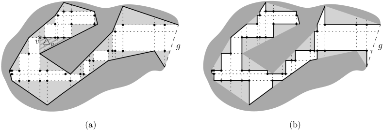
Figure 12: Illustration to how to construct $\mathcal{P}_{rect}$. (a) A bay $A$ with gate $g$ and the decomposition $\mathcal{D}$ inside $A$. The dark gray region depicts the hole of $\mathcal{P}$ bounding $A$, coastal cells of $\mathcal{D}$ intersecting $\partial A$ are shaded by light gray color, and black dots are vertices in $V_{c}\setminus\partial\mathcal{P}$. One of those in $V_{c}$ is labeled $v$ and its triangle $\triangle_{v}$ is highlighted. (b) The rectified polygonal domain $\mathcal{P}_{rect}$ obtained by expanding the hole into $\triangle_{v}$ for all $v\in V_{c}$. The boundary of $\mathcal{P}_{rect}$ is depicted by solid segments. Here, the edges of $A$ are ordered in the counter-clockwise order.

In the following, we focus on how to compute $d(v,v^{\prime})$ for all $v,v^{\prime}\in V_{c}\setminus\partial\mathcal{P}$. Let $e_{1},\ldots,e_{n}$ be the edges of $\mathcal{P}$ in an arbitrary order. We modify the original polygonal domain $\mathcal{P}$ to obtain the rectified polygonal domain $\mathcal{P}_{rect}$ as follows. For each $i=1,\ldots,n$, we define $V_{i}$ to be the set of all vertices $v\in(V_{c}\setminus\partial\mathcal{P})\setminus(V_{1}\cup\cdots\cup V_{i-1})$ such that $v\in V_{\sigma}$ for some coastal cell $\sigma\in\mathcal{D}_{\!f}$ with $\partial\sigma\cap e_{i}\neq\emptyset$. For each $v\in V_{i}$, we shoot two rays from $v$, vertical and horizontal, towards $e_{i}$ until each hits $e_{i}$. Let $\triangle_{v}$ be the triangle formed by $v$ and the two points on $e_{i}$ hit by the rays. Since $v$ is a vertex of a cell of $\mathcal{D}$ facing $e_{i}$, by the construction of $\mathcal{D}$, the two rays must hit $e_{i}$ and thus the triangle $\triangle_{v}$ is well defined. We then expand each hole of $\mathcal{P}$ into the triangles $\triangle_{v}$ for all $v\in V_{c}\setminus\partial\mathcal{P}$. Let $\mathcal{P}_{rect}$ be the resulting polygonal domain; that is, every triangle $\triangle_{v}$ is regarded as an obstacle in $\mathcal{P}_{rect}$. We also add all those in $V_{c}\setminus\partial\mathcal{P}$ into $\mathcal{P}_{rect}$ as obstacle vertices. See Figure 12. Observe that $\mathcal{P}_{rect}$ is a subset of $\mathcal{P}$ as subsets of $\mathbb{R}^{2}$ and all those in $V_{c}\setminus\partial\mathcal{P}$ lie on the boundary of $\mathcal{P}_{rect}$ as its obstacle vertices. For any two points $s,t\in\mathcal{P}_{rect}$, let $d_{rect}(s,t)$ be the $L_{1}$ geodesic distance between $s$ and $t$ in $\mathcal{P}_{rect}$.

We then claim the following:

For any $s,t\in\mathcal{P}_{rect}$, it holds that $d(s,t)=d_{rect}(s,t)$.

Suppose that the claim is true. The construction of $\mathcal{P}_{rect}$ can be done in $O(n^{2})$ time. Then, for any $v\in V_{c}\setminus\partial\mathcal{P}$, we compute the shortest path map $S\!P\!M_{rect}(v)$ in the rectified domain $\mathcal{P}_{rect}$ and obtain $d(v,v^{\prime})$ for all other $v^{\prime}\in V_{c}\setminus\partial\mathcal{P}$. Since $\mathcal{P}_{rect}$ has $h$ holes and $O(n)$ vertices by our construction of $\mathcal{P}_{rect}$, this task can be done in $O(n+h\log h)$ time [9, 11]. At last, case (iii) can be processed in total $O(n^{2}+nh\log h)$ time.

We now prove the claim, as follows.

Proof of the claim. For any $v\in V_{c}\setminus\partial\mathcal{P}$, the triangle $\triangle_{v}$ is well defined. We call a triangle $\triangle_{v}$ maximal if there is no other $\triangle_{v^{\prime}}$ with $\triangle_{v}\subset\triangle_{v^{\prime}}$. Note that any two maximal triangles are interior-disjoint but may share a portion of their sides. Indeed, $\mathcal{P}\setminus\mathcal{P}_{rect}$ is the union of all maximal triangles $\triangle_{v}$. Pick any connected component $C$ of $\mathcal{P}\setminus\mathcal{P}_{rect}$. The set $C$ is either a maximal triangle $\triangle_{v}$ itself or the union of two maximal triangles that share a portion of their sides by our construction of $\mathcal{P}_{rect}$ and of $\mathcal{D}$. In either case, observe that the portion $\partial C\setminus\partial\mathcal{P}$ is a monotone path.

Consider any $s,t\in\mathcal{P}_{rect}$ and any shortest $s$-$t$ path $\pi$ in $\mathcal{P}$, that is, $d(s,t)=|\pi|$. If $\pi$ lies inside $\mathcal{P}_{rect}$, then we are done since the $L_{1}$ length of any $s$-$t$ path inside $\mathcal{P}_{rect}$ is at least $d(s,t)$. Otherwise, $\pi$ may cross a number of connected components of $\mathcal{P}\setminus\mathcal{P}_{rect}$. Pick any such connected component $C$ that is crossed by $\pi$. Let $p$ and $q$ be the first and the last points on $\partial C$ we encounter when walking along $\pi$ from $s$ to $t$. Since $\partial C\setminus\partial\mathcal{P}$ is monotone as observed above, the path $\pi_{pq}$ along the boundary of $C$ is also monotone. By Fact 1, $|\pi_{pq}|=|\overline{pq}|$ and thus we can replace the subpath of $\pi$ between $p$ and $q$ by $\pi_{pq}$ without increasing the $L_{1}$ length. The resulting path thus has length equal to $|\pi|$ and avoids the interior of $C$. We repeat the above procedure for all such connected components $C$ crossed by $\pi$. At last, the final path $\pi^{\prime}$ has length equal to $|\pi|$ and avoids the interior of $\mathcal{P}\setminus\mathcal{P}_{rect}$. That is, $\pi^{\prime}$ is a $s$-$t$ path in $\mathcal{P}_{rect}$ with $|\pi^{\prime}|=|\pi|=d(s,t)$. Since $d_{rect}(s,t)\geq d(s,t)$ in general, $\pi^{\prime}$ is an $L_{1}$ shortest $s$-$t$ path in $\mathcal{P}_{rect}$, and hence $d_{rect}(s,t)=d(s,t)$.

This proves the above claim.

Consequently, the total time complexity is bounded by

$$O(nh^{2}+h^{4})+O(n^{2}+nh\log h)=O(n^{2}+nh^{2}+h^{4})=O(n^{2}+h^{4}).$$

The lemma thus follows.

Our algorithms for computing the diameter and center are summarized in the proof of the following theorem.

Theorem 4.17.

The $L_{1}$ geodesic diameter and center of $\mathcal{P}$ can be computed in $O(n^{2}+h^{4})$ and $O((n^{4}+n^{2}h^{4})\alpha(n))$ time, respectively.

Proof 4.18.

We first discuss the diameter algorithm, whose correctness follows directly from Lemma 4.14.

After the execution of the procedure of Lemma 4.15 as a preprocessing, our algorithm considers three cases for two cells $\sigma,\sigma^{\prime}\in\mathcal{D}_{\!f}$: (i) both are oceanic, (ii) both are coastal, or (iii) $\sigma$ is coastal and $\sigma^{\prime}$ is oceanic. In either case, we apply Lemma 4.12.

For case (i), we have $O(h^{2})$ oceanic cells and the total complexity is $\sum_{\sigma\in\mathcal{D}_{\!\mathcal{M}}}n_{\sigma}=O(n+h^{2})$. Thus, the total time for case (i) is bounded by

$$\sum_{\sigma\in\mathcal{D}_{\!\mathcal{M}}}\sum_{\sigma^{\prime}\in\mathcal{D}_{\!\mathcal{M}}}O(n_{\sigma}n_{\sigma^{\prime}})=\sum_{\sigma\in\mathcal{D}_{\!\mathcal{M}}}O(n_{\sigma}(n+h^{2}))=O((n+h^{2})^{2})=O(n^{2}+h^{4}).$$

For case (ii), we have $O(n)$ coastal cells in $\mathcal{D}_{\!\mathcal{M}}$ and their total complexity is $O(n)$ since they are all trapezoidal. Thus, the total time for case (ii) is bounded by $O(n^{2})$.

For case (iii), we fix a coastal cell $\sigma\in\mathcal{D}_{\!f}$ and iterate over all oceanic cells $\sigma^{\prime}\in\mathcal{D}_{\!\mathcal{M}}$, after an $O(n)$-time preprocessing, as done in the proof of Lemma 4.12. For each $\sigma$, we take $O(n+h^{2})$ time since $\sum_{\sigma\in\mathcal{D}_{\!\mathcal{M}}}n_{\sigma}=O(n+h^{2})$. Thus, the total time for case (iii) is bounded by $O(n^{2}+nh^{2})=O((n+h^{2})^{2})=O(n^{2}+h^{4})$.

Next, we discuss our algorithm for computing a geodesic center of $\mathcal{P}$. We consider $O(n^{2})$ cells $\sigma\in\mathcal{D}$ and compute all the $\sigma$-constrained centers. As a preprocessing, we spend $O(n^{4})$ time to compute the geodesic distances $d(v,v^{\prime})$ for all pairs of vertices of $\mathcal{D}$ by Lemma 2.5. Fix a cell $\sigma\in\mathcal{D}$. For all $\sigma^{\prime}\in\mathcal{D}_{\!f}$, we compute the geodesic distance function $d$ restricted to $\sigma\times\sigma^{\prime}$ by applying Lemma 4.12. As in Section 2, compute the graph of $R_{\sigma^{\prime}}(q)=\max_{p\in\sigma^{\prime}}d(p,q)$ by projecting the graph of $d$ over $\sigma\times\sigma^{\prime}$, and take the upper envelope of the graphs of $R_{\sigma^{\prime}}$ for all $\sigma^{\prime}\in\mathcal{D}_{\!f}$. By Lemma 4.12, we have an analogue of Lemma 2.8 and thus a $\sigma$-constrained center can be computed in $O(m^{2}\alpha(m))$ time, where $m$ denotes the total complexity of all $R_{\sigma^{\prime}}$. Lemma 4.12 implies that $m=O(n+h^{2})$.

For the time complexity, note that $\sum_{\sigma\in\mathcal{D}_{\!\mathcal{M}}}n_{\sigma}=O(n+h^{2})$ and $\sum_{\sigma\in\mathcal{D}_{\!f}\setminus\mathcal{D}_{\!\mathcal{M}}}n_{\sigma}=O(n)$. Since any cell in $\mathcal{D}$ is either a triangle or a trapezoid, its complexity is $O(1)$. Thus, for each $\sigma\in\mathcal{D}$, by Lemma 4.12, computing a $\sigma$-constrained center takes $O((n+h^{2})^{2}\alpha(n))$ time, after an $O(n^{4})$-time preprocessing (Lemma 2.5). Iterating over all $\sigma\in\mathcal{D}$ takes $O(n^{2}(n+h^{2})^{2}\alpha(n))=O((n^{4}+n^{2}h^{4})\alpha(n))$ time.

5 Conclusions

We gave efficient algorithms for computing the $L_{1}$ geodesic diameter and center of a polygonal domain. In particular, we exploited the extended corridor structure to make the running times depend on the number of holes in the domain (which may be much smaller than the number of vertices). It would be interesting to find further improvements to the algorithms in hopes of reducing the worst-case running times; it would also be interesting to prove non-trivial lower bounds on the time complexities of the problems.

Acknowledgements.

Work by S.W. Bae was supported by Basic Science Research Program through the National Research Foundation of Korea (NRF) funded by the Ministry of Science, ICT & Future Planning (2013R1A1A1A05006927), and by the Ministry of Education (2015R1D1A1A01057220). M. Korman is partially supported by JSPS/MEXT Grant-in-Aid for Scientific Research Grant Numbers 12H00855 and 15H02665. J. Mitchell acknowledges support from the US-Israel Binational Science Foundation (grant 2010074) and the National Science Foundation (CCF-1018388, CCF-1526406). Y. Okamoto is partially supported by JST, CREST, Foundation of Innovative Algorithms for Big Data and JSPS/MEXT Grant-in-Aid for Scientific Research Grant Numbers JP24106005, JP24700008, JP24220003, and JP15K00009. V. Polishchuk is supported in part by Grant 2014-03476 from the Sweden’s innovation agency VINNOVA and the project UTM-OK from the Swedish Transport Administration Trafikverket. H. Wang was supported in part by the National Science Foundation (CCF-1317143).

References

- [1] H.-K. Ahn, L. Barba, P. Bose, J.-L. De Carufel, M. Korman, and E. Oh. A linear-time algorithm for the geodesic center of a simple polygon. In Proc. of the 31st Symposium on Computational Geometry, pages 209–223, 2015.
- [2] B. Aronov. On the geodesic Voronoi diagram of point sites in a simple polygon. Algorithmica, 4(1–4):109–140, 1989.
- [3] T. Asano and G. Toussaint. Computing the geodesic center of a simple polygon. Technical Report SOCS-85.32, McGill University, Montreal, Canada, 1985.
- [4] S.W. Bae, M. Korman, and Y. Okamoto. The geodesic diameter of polygonal domains. Discrete and Computational Geometry, 50:306–329, 2013.
- [5] S.W. Bae, M. Korman, and Y. Okamoto. Computing the geodesic centers of a polygonal domain. In Proc. of the 26th Canadian Conference on Computational Geometry, 2014. Journal version to appear in Computational Geometry: Theory and Applications, http://dx.doi.org/10.1016/j.comgeo.2015.10.009.
- [6] S.W. Bae, M. Korman, Y. Okamoto, and H. Wang. Computing the geodesic diameter and center of a simple polygon in linear time. Computational Geometry: Theory and Applications, 48:495–505, 2015.
- [7] R. Bar-Yehuda and B. Chazelle. Triangulating disjoint Jordan chains. International Journal of Computational Geometry and Applications, 4(4):475–481, 1994.
- [8] B. Chazelle. A theorem on polygon cutting with applications. In Proc. of the 23rd Annual Symposium on Foundations of Computer Science, pages 339–349, 1982.
- [9] D.Z. Chen and H. Wang. A nearly optimal algorithm for finding shortest paths among polygonal obstacles in the plane. In Proc. of the 19th European Symposium on Algorithms, pages 481–492, 2011.
- [10] D.Z. Chen and H. Wang. Computing the visibility polygon of an island in a polygonal domain. In Proc. of the 39th International Colloquium on Automata, Languages and Programming, pages 218–229, 2012. Journal version published online in Algorithmica, 2015.
- [11] D.Z. Chen and H. Wang. shortest path queries among polygonal obstacles in the plane. In Proc. of the 30th Symposium on Theoretical Aspects of Computer Science, pages 293–304, 2013.
- [12] H. Edelsbrunner, L.J. Guibas, and M. Sharir. The upper envelope of piecewise linear functions: Algorithms and applications. Discrete and Computational Geometry, 4:311–336, 1989.
- [13] L.J. Guibas, J. Hershberger, D. Leven, M. Sharir, and R.E. Tarjan. Linear-time algorithms for visibility and shortest path problems inside triangulated simple polygons. Algorithmica, 2(1-4):209–233, 1987.
- [14] J. Hershberger and J. Snoeyink. Computing minimum length paths of a given homotopy class. Computational Geometry: Theory and Applications, 4(2):63–97, 1994.
- [15] J. Hershberger and S. Suri. Matrix searching with the shortest-path metric. SIAM Journal on Computing, 26(6):1612–1634, 1997.
- [16] R. Inkulu and S. Kapoor. Planar rectilinear shortest path computation using corridors. Computational Geometry: Theory and Applications, 42(9):873–884, 2009.
- [17] S. Kapoor, S.N. Maheshwari, and J.S.B. Mitchell. An efficient algorithm for Euclidean shortest paths among polygonal obstacles in the plane. Discrete and Computational Geometry, 18(4):377–383, 1997.
- [18] J.S.B. Mitchell. An optimal algorithm for shortest rectilinear paths among obstacles. In the 1st Canadian Conference on Computational Geometry, 1989.
- [19] J.S.B. Mitchell. shortest paths among polygonal obstacles in the plane. Algorithmica, 8(1):55–88, 1992.
- [20] E. Papadopoulou and D.T. Lee. A new approach for the geodesic Voronoi diagram of points in a simple polygon and other restricted polygonal domains. Algorithmica, 20(4):319–352, 1998.
- [21] R. Pollack, M. Sharir, and G. Rote. Computing the geodesic center of a simple polygon. Discrete and Computational Geometry, 4(1):611–626, 1989.
- [22] S. Schuierer. Computing the -diameter and center of a simple rectilinear polygon. In Proc. of the International Conference on Computing and Information, pages 214–229, 1994.
- [23] S. Suri. Computing geodesic furthest neighbors in simple polygons. Journal of Computer and System Sciences, 39:220–235, 1989.
- [24] H. Wang. On the geodesic centers of polygonal domains. In Proc. of the 24th European Symposium on Algorithms, pages 77:1–77:17, 2016.