Finite element method and isogeometric analysis in electronic structure calculations: convergence study

Abstract

We compare convergence of isogeometric analysis (IGA), a spline modification of finite element method (FEM), with FEM in the context of our real space code for ab-initio electronic structure calculations of non-periodic systems. The convergence is studied on simple sub-problems that appear within the density functional theory approximation to the Schrödinger equation: the Poisson problem and the generalized eigenvalue problem. We also outline the complete iterative algorithm seeking a fixed point of the charge density of a system of atoms or molecules, and study IGA/FEM convergence on a benchmark problem of nitrogen atom.

1 Introduction

The electronic structure calculations are a rigorous tool for predicting and understanding important properties of materials, such as elasticity, hardness, electric and magnetic properties, etc. Those properties are tightly bound to the notion of the total internal energy of a system of atoms — a crucial quantity to compute, and to determine its sensitivity w.r.t. various parameters, e.g., the atomic positions in order to reach a stable arrangement.

Our team is developing a real space code [34] for electronic structure calculations based on

• the density functional theory (DFT), [15, 27, 23, 28];

• the environment-reflecting pseudopotentials [33];

• a weak solution of the Kohn-Sham equations [19].

The code is based on the open source finite element package SfePy [8] (Simple Finite Elements in Python, http://sfepy.org), which is a general package for solving (systems of) partial differential equations (PDEs) by the finite element method (FEM), cf. [32]. Recently, it has been extended with the isogeometric analysis (IGA) [11] is a spline-based modification of FEM. The key motivation for this extension, besides interesting convergence properties [21] in eigenvalue problems, was the possibility of a continuous field approximation with a high global continuity on a simple domain — a single NURBS (Non-uniform Rational B-spline) patch. This feature is crucial for an efficient evaluation of the sensitivity of the total energy w.r.t. a parameter, also called the Hellman-Feynman forces (HFF) [9].

Recently, using FEM and its variants in electronic structure calculation context is pursued by a growing number of groups, cf. [13], where the $hp$-adaptivity is discussed, [25, 26] where spectral finite elements as well as the $hp$-adaptivity are considered, or [24], where NURBS-based FEM is applied.

IGA is a modification of FEM which employs shape functions of different spline types such as B-splines, NURBS [29]), T-splines [2], etc. It was successfully employed for numerical solutions of various physical and mathematical problems, such as fluid dynamics, diffusion and other problems of continuum mechanics [11, 20, 21]. The theoretical works relating to the convergence behaviour of IGA have been published in [3, 6, 4, 22].

The drawbacks of using IGA, as reported in [21], concern mainly the increased computational cost of the numerical integration and assembling. Also, because of the higher global continuity, the assembled matrices have more nonzero entries than the matrices corresponding to the $C^{0}$ FEM basis. A comparison study of IGA and FEM matrix structures, the cost of their evaluation, and mainly the cost of direct and iterative solvers in IGA has been presented by [10] and [30].

In this paper we compare numerical convergence properties of FEM and IGA using problems originating from various stages of our electronic structure calculation algorithm, in order to assess the applicability of IGA for our purposes. It is structured as follows: in Section 2 we provide a light-weight introduction to the topic of electronic structure calculations, in Section 3 the used discretization methods (FEM and IGA) are presented. Finally, in Section 4 the numerical convergence results are presented: first for several Poisson problems because the Poisson problem solution is an important part of the algorithm used for calculation of the electrostatic potential (see below); then several eigenvalue problems corresponding to simple quantum mechanical systems with a similar matrix structure to that of the complete problem; and finally, for the overall algorithm.

2 Electronic structure calculations

Let us briefly introduce the topic of electronic structure calculations. The systems of atoms and molecules are described in the most general form by the many-particle Schrödinger equation, cf. [23],

$$H\Psi(e_{1},e_{2},\dots,e_{n})=\varepsilon\Psi(e_{1},e_{2},\dots,e_{n})\;,$$ (1)

where $H$ is the Hamiltonian (energy operator) of the system, $e_{i}$ the particles (e.g. electrons) and $\varepsilon$ the energy of the state $\Psi$. The equation (1) is, however, too complicated to solve, even for three electrons. Among the techniques reducing this complexity, we use the DFT approach [15]. The DFT allows decomposing the many-particle Schrödinger equation into the one-electron Kohn-Sham equations [19]. Using atomic units they can be written in the common form

$$\left(-\frac{1}{2}\nabla^{2}+V_{\text{H}}(\bm{r})+V_{\text{xc}}(\bm{r})+\hat{V}(\bm{r})\right)\psi_{i}=\varepsilon_{i}\psi_{i}\;,$$ (2)

which provide the orbitals $\psi_{i}$ that reproduce, with the weights of occupations $n_{i}$, the charge density $\rho$ of the original interacting system, as

$$\rho(\bm{r})=\sum_{i}^{N}n_{i}|\psi_{i}(\bm{r})|^{2}\;.$$ (3)

$\hat{V}$ is a (generally) non-local Hermitian operator representing the effective ionic potential for electrons. In the present case, within pseudopotential approach, $\hat{V}$ represents core electrons, separated from valence electrons, together with the nuclear charge. $V_{\text{xc}}$ is the exchange-correlation potential describing the non-coulomb electron-electron interactions. The exact potential is not known, so we use local-density aproximation (LDA) of this potential [23], where the potential is a function of charge density at a given point. $V_{\text{H}}$ is the electrostatic potential obtained as a solution to the Poisson equation. The Poisson equation for $V_{\text{H}}$ has the charge density $\rho$ at its right-hand side and is as follows:

$$\Delta V_{\text{H}}=4\pi\rho\;.$$ (4)

Denoting the total potential $V:=V_{\text{H}}+V_{\text{xc}}+\hat{V}$, we can write, using Hartree atomic units,

$$\left(-\frac{1}{2}\nabla^{2}+V(\bm{r})\right)\psi_{i}=\varepsilon_{i}\psi_{i}\;.$$ (5)

Note that the above mentioned eigenvalue problem is highly non-linear, as the potential $V$ depends on the orbitals $\psi_{i}$. Therefore an iterative scheme is needed, defining the DFT loop for attaining a self-consistent solution.

2.1 DFT loop

For the global convergence of the DFT iteration we use the standard algorithm outlined in Fig. 1. The purpose of the DFT loop is to find a self-consistent solution — a fixed point of a function of the charge density $\rho$. For this task, a variety of nonlinear solvers can be used. We use Broyden-type quasi-Newton solvers applied to

$$DFT(\rho^{i})-\rho^{i}=\rho^{i+1}-\rho^{i}=0\;,$$ (6)

where $DFT$ denotes a single iteration of the DFT loop.

Figure 1: DFT, iterative self-consistent scheme.

After the DFT loop convergence is achieved, the derived quantities, particularly the total energy, are computed. By minimizing the total energy as a function of atomic positions, the equilibrium atomic positions can be found. Therefore the DFT loop itself can be embedded into an outer optimization loop, where the objective function gradients are the HFF.

2.2 Total Energy and Forces Acting on Atoms

The total energy of the system can be obtained within DFT as the sum of the ion-ion interaction energy (i.e. energy of electrostatic interations among nuclei), the kinetic energy of electrons, the electron-ion interaction energy, the electron-electron electrostatic interaction energy and the exchange and correlation energy that reflect the fact that electron, as any fermions, satisfy the Pauli principle and the fact that electrons, like any quantum-mechanical particles, are indistinguishable in principle (i.e. via an exchange of two electrons we don’t get another quantum state). The terms mentioned above, respectively, can be expressed as

$$E_{\rm tot}=\frac{1}{2}\sum_{a,a^{\prime}\neq a}\frac{Z_{\alpha}Z_{\alpha^{\prime}}}{\left|\tau_{\alpha}-\tau_{\alpha^{\prime}}\right|}+\sum_{i}n_{i}\int\!{\rm d}\mathbf{r}\;\;\psi^{*}_{i}(\mathbf{r})\left(-\frac{1}{2}\nabla^{2}\right)\psi_{i}(\mathbf{r})+$$

$$+\int\!{\rm d}\mathbf{r}\;\rho(\mathbf{r})\hat{V}(\mathbf{r})+\frac{1}{2}\int\!\!\!\int\!{\rm d}\mathbf{r}\;\frac{\rho(\mathbf{r})\rho(\mathbf{r}^{\prime})}{\left|\mathbf{r}-\mathbf{r}^{\prime}\right|}+\int\!{\rm d}\mathbf{r}\;\rho(\mathbf{r})V_{\rm xc}^{\rm E}(\mathbf{r};\rho)\;,$$ (7)

where $\alpha$ refers to atomic sites and $Z$ stands for the ionic charge of the nucleus (or of the core, in case of pseudopotentials). $V_{\rm xc}^{\rm E}(\mathbf{r};\rho)$ denotes the exchange-correlation energy functional of the charge density related to the exchange-correlation potential via

$$V_{\rm xc}=\frac{\partial}{\partial\rho}\left(V_{\rm xc}^{\rm E}\right)\;.$$ (8)

The force acting on atom $\alpha$ is equal to the derivative of the total energy functional with respect to an infinitesimal displacement of this atom $\delta\tau_{\alpha}$:

$${\mathbf{F}}^{\alpha}=-\frac{\delta E}{\delta\tau_{\alpha}}$$ (9)

Making use of the Hellmann-Feynman theorem that relates the derivative of the total energy with respect to a parameter $\lambda$, to the expectation value of the derivative of the Hamiltonian operator w.r.t. the same parameter

$$\frac{{\rm d}E}{{\rm d}\lambda}=\left\langle\psi^{*}_{\lambda}\left|\frac{{\rm d}\hat{H}_{\lambda}}{{\rm d}\lambda}\right|\psi_{\lambda}\right\rangle\rm,$$ (10)

within the density functional theory we can write

$${\mathbf{F}}^{\alpha}={\mathbf{F}}^{\alpha}_{\rm HF,es}-\frac{\left(\sum_{i}n_{i}\delta\varepsilon_{i}-\int\rho({\mathbf{r}})\delta\left[\hat{V}+V_{\rm H}+V_{\rm xc}\right]\!({\mathbf{r}}){\rm d}^{3}{\mathbf{r}}\right)}{\delta\tau_{\alpha}}$$ (11)

where the first term is the electrostatic Hellmann-Feynman force (formed by the sum over all the atoms $\beta\neq\alpha$ of electrostatic forces between the charges of atomic nuclei $Z_{\alpha}$ and $Z_{\beta}$ and by the force acting on the charge $Z_{\alpha}$ in the charge density $\rho$)

$${\mathbf{F}}^{\alpha}_{\rm HF,es}=Z_{\alpha}\frac{{\rm d}}{{\rm d}\tau_{\alpha}}\left(-\sum_{\beta\neq\alpha}\frac{Z_{\beta}}{|\tau_{\alpha}-\tau_{\beta}|}+\int\frac{\rho({\mathbf{r}})}{|\tau_{\alpha}-{\mathbf{r}}|}d^{3}{\mathbf{r}}\right)$$ (12)

and the second term in Eq.(11), is the “Pulay” force, also known as “incomplete basis set” force, that contains the corrections that depend on technical details of the calculation and can be extremely complicated to evaluate for some non-tirivial types of bases. By means of the fixed basis independent of atomic position and via the wave function $\psi_{i}$ continuity up to second derivatives, we can get rid of this troublesome term. Even without this term, the evaluation of pure HF-force in case of non-local separable pseudopotentials acting in the $l-$projected (via the spheriacal harmonics) subspaces,

$${\mathbf{F}}^{\alpha}_{\rm HF,es}=\frac{\partial}{\partial\tau_{\alpha}}\left(\int\!{\rm d}\mathbf{r}\;\rho\hat{V}^{\rm\scriptscriptstyle LOC}\right)+\frac{\partial}{\partial\tau_{\alpha}}\left(\sum_{i}n_{i}\int{\rm d}\mathbf{r}\;\psi^{*}_{i}\hat{V}^{\rm\scriptscriptstyle NL}\psi_{i}\right)$$

$$+\frac{\partial}{\partial\tau_{\alpha}}\left(\frac{1}{2}\int{\rm d}\mathbf{r}\;\rho^{\rm\scriptscriptstyle\stackrel{{\scriptstyle ion}}{{LOC}}}\hat{V}^{\rm\scriptscriptstyle LOC}\right)-\frac{\partial}{\partial\tau_{\alpha}}\left(\frac{1}{2}\sum_{a}\int{\rm d}\mathbf{r}\;\rho^{\rm\scriptscriptstyle\stackrel{{\scriptstyle ion}}{{LOC}}}_{a}\hat{V}^{\rm\scriptscriptstyle LOC}_{\alpha}\right)\;,$$ (13)

where the superscripts ^LOC and ^NL denote the local and non-local pseudopotential parts, respectively, and

$$\rho^{\rm\scriptscriptstyle\stackrel{{\scriptstyle ion}}{{LOC}}}(\mathbf{x})=-\frac{1}{4\pi}\nabla^{2}\hat{V}^{\rm\scriptscriptstyle LOC}(\mathbf{x})\;,$$ (14)

might be non-trivial, as it was shown by Ihm, Zunger and Cohen[18] (for more details see e.g. [36], [35], [14]). But, anyway, it seems to be much more acceptable for practical use than the evaluating the additional Pulay term within finite-element basis would be.

3 Discretization methods

Before presenting key points of FEM and IGA, our problem needs to be reinstated in a weak form, usual in the finite element setting.

3.1 Weak formulation

Let us denote $H^{1}(\Omega)$ the usual Sobolev space of functions with $L^{2}$ integrable derivatives and $H^{1}_{0}(\Omega)=\{u\in H^{1}(\Omega)|u=0\mbox{ on }\partial\Omega\}$.

The eigenvalue problem (5) can be rewritten using the weak formulation: find functions $\psi_{i}\in H^{1}(\Omega)$ such that for all $v\in H^{1}_{0}(\Omega)$ holds

$$\int_{\Omega}\frac{1}{2}\nabla\psi_{i}\cdot\nabla v\ {\rm d}V+\int_{\Omega}vV\psi_{i}\ {\rm d}V=\varepsilon_{i}\int_{\Omega}v\psi_{i}\ {\rm d}V+\oint_{\partial\Omega}\frac{1}{2}\frac{{\rm d}\psi_{i}}{{\rm d}\bm{n}}\ {\rm d}S\;.$$ (15)

If the solution domain $\Omega$ is sufficiently large, the last term can be neglected. The Poisson equation (4) has the following weak form:

$$\int_{\Omega}\nabla v\cdot\nabla V_{\text{H}}=4\pi\int_{\Omega}\rho v\;.$$ (16)

Equations (15), (16) then need to be discretized — the continuous fields are approximated by discrete fields with a finite set of degrees of freedom (DOFs) and a basis, typically piece-wise polynomial:

$$u(\bm{r})\approx u^{h}(\bm{r})=\sum_{k=1}^{N}u_{k}\phi_{k}(\bm{r})\mbox{ for }\bm{r}\in\Omega\;,$$ (17)

where $u$ is a continuous field ($\psi$, $v$, $V_{H}$ in our equations), $u_{k}$, $k=1,2,\dots,N$ are the discrete DOFs and $\phi_{k}$ are the basis functions. From the computational point of view it is desirable that the basis functions have a small support, so that the resulting system matrix is sparse.

Substituting (17) into (15) leads to the matrix form of the Kohn-Sham eigenvalue problem:

$$\left(\bm{K}+\bm{V}(\psi_{i})\right)\psi_{i}=\varepsilon_{i}\bm{M}\psi_{i}\;,$$ (18)

where

$$\bm{K}=\{K_{ij}\}\equiv\int_{\Omega_{h}}\nabla\phi_{i}\nabla\phi_{j}\;,$$

$$\bm{V}(\psi_{i})=\{V_{ij}\}\equiv\int_{\Omega_{h}}\phi_{i}V(\psi_{i})\phi_{j}\;,$$

$$\bm{M}=\{M_{ij}\}\equiv\int_{\Omega_{h}}\phi_{i}\phi_{j}\;.$$

Similarly, the matrix form of the Poisson problem (16) is:

$$\bm{K}\bm{u}=\bm{f}\;,$$ (19)

where $V_{\text{H}}(\bm{r})\approx\sum_{k=1}^{N}u_{k}\phi_{k}(\bm{r})$ and $\bm{f}=\{f_{i}\}\equiv 4\pi\int_{\Omega_{h}}\rho\phi_{i}$.

3.2 Finite element method

In the FEM the discretization process involves the discretization of the domain $\Omega$ — it is replaced by a polygonal domain $\Omega_{h}$ that is covered by small non-overlapping subdomains called elements (e.g. triangles or quadrilaterals in 2D, tetrahedrons or hexahedrons in 3D), cf. [17, 32]. The elements form a finite element mesh.

The basis functions are defined as piece-wise polynomials over the individual elements, have a small support and are typically globally $C^{0}$ continuous. The discretized equations are evaluated over the elements as well to obtain local matrices or vectors that are then assembled into a global sparse system. The evaluation usually involves a numerical integration on a reference element, and a mapping to individual physical elements [17, 32]. The nodal basis of Lagrange interpolation polynomials or the hierarchical basis of Lobatto polynomials can be used in our code.

3.3 Isogeometric analysis

The basis functions in IGA are formed directly from the CAD geometrical description in terms of NURBS patches, without the intermediate FE mesh — the meshing step is removed, which is one of its principal advantages. A NURBS patch is a single NURBS object — a linear combination of control points $\bm{P}=\{\bm{P}_{A}\}_{A=1}^{N}$ (or unknown field coefficients) and NURBS basis functions $R_{A,p}(\underline{\xi})$, where $p$ is the NURBS solid degree and $\underline{\xi}=\{\xi_{1},\dots,\xi_{D}\}$ are the parametric coordinates. Thus, a d-dimensional geometric domain is defined by

$$\bm{r}(\underline{\xi})=\sum_{A=1}^{n}\bm{P}_{A}R_{A,p}(\underline{\xi})=\bm{P}^{T}\bm{R}(\underline{\xi})\;.$$ (20)

If $d>1$, the NURBS solid can be defined as a tensor product of univariate NURBS curves. The basic properties of the B-spline basis functions can be found in [29].

The same NURBS basis is used also for the approximation of a continuous field $u$ ($\psi$, $v$, $V_{H}$ in our equations):

$$\bm{u}(\underline{\xi})=\sum_{A=1}^{n}u_{A}R_{A,p}(\underline{\xi})\;,$$ (21)

where $u_{A}$ are the unknown DOFs — coefficients of the basis in the linear combination.

Our implementation [7] uses a variant of IGA based on Bézier extraction operators [5] that is suitable for inclusion into existing FE codes. The code itself does not see the NURBS description at all. It is based on the observation that repeating a knot in the knot vector decreases continuity of the basis in that knot by one. This can be done in such a way that the overall shape remains the same, but the “elements” appear naturally as given by non-zero knot spans. The final basis restricted to each of the elements is formed by the Bernstein polynomials $\bm{B}$. The assembling of matrices and vectors on resulting from (18) then proceeds in the usual FE sense (cf. [5]):

1. Setup points $\xi_{q}$ for numerical quadrature on a reference element.

2. Loop over elements of the Bézier “mesh” (given by knot spans).

3. On each element $e$:

   1. Evaluate the Bernstein basis $\bm{B}(\xi_{q})|_{e}$,

   2. Reconstruct the original NURBS basis: $\bm{R}(\xi_{q})|_{e}=\bm{C}|_{e}\bm{B}(\xi_{q})|_{e}$, using the Bézier extraction operator $\bm{C}$, that is local to element $e$.

   3. Evaluate element contributions to the global matrix.

   4. Assemble using the original DOF connectivity.

The Bézier extraction matrices $\bm{C}$ are pre-computed for a NURBS patch domain using an efficient algorithm that employs the tensor-product nature of the patch [5], and then reused in all subsequent computations on that domain.

4 Results

The electronic structure calculations described in Section 2 involve solving the following two sub-problems:

• the Poisson equation (16) for the potential $V_{H}$,

• and the generalized eigenvalue problem (15).

Below we compare the convergence of FEM and IGA when applied to the two sub-problems, as well as to the entire algorithm of the DFT loop (6).

All computations were done on a tensor-product domain, with varying number of vertices/knots along an edge.

We are interested in convergence w.r.t. three parameters:

• The number of vertices/knots along the domain edge $N_{e}$ provides insight into the work necessary to integrate over the domain, because $(N_{e}-1)^{d}$ is equal to the number of elements/Bézier elements. Also, the element size $h$ can be obtained as $h=1/((N_{e}-1)$.

• The number of non-zero entries in the matrices $N_{nz}$ that corresponds to the cost of matrix-vector products, and hence the cost of a single linear/eigenvalue problem solver iteration.

• The total number of degrees of freedom $N_{dof}$, i.e. the size of the matrices, which is related to the difficulty of solving the Poisson equation (16) or the eigenvalue problem (15).

Thus a higher $N_{e}$ indicates a higher cost of assembling the matrices, while higher $N_{nz}$ and $N_{dof}$ mean a more difficult problem solution.

4.1 Poisson’s equation with manufactured solutions

In the method of manufactured solutions, cf. [22], a solution $u(\bm{r})$ is made up and the left-hand side operator (the Laplace operator here) is applied to obtain the corresponding right-hand side $g(\bm{r})\equiv\Delta u(\bm{r})$. The function $g(\bm{r})$ is then used as the right-hand side in the numerical solution, while $u(\bm{r})$ for $\bm{r}\in\Gamma$ is applied as the Dirichlet boundary condition on the whole domain surface $\Gamma$.

Several analytic formulas were considered in 1D, 2D and 3D. The domain was a unit cube (or square): $\Omega\equiv[-0.5,0.5]^{d}$, $d=1,2,3$. The discretization parameters are summarized in Tab. 1.

In the FEM setting, the Lagrange basis with 1D polynomial orders 1, 2 and 3 and the uniform discretization were used. In the IGA context, the B-spline basis with 1D degrees 1, 2 and 3, and the approximation with uniformly distributed knots, were used. We also varied the global continuity of the B-spline basis: up to $C^{2}$, depending on the B-spline degree. Note that the B-spline basis with $C^{0}$ continuity is equivalent to the FEM basis.

dimension	$N_{e}$	solver
1D	100, 200, 500, 1000, 2000	direct
2D	5, 10, 15, 25, 40, 60	iterative
3D	5, 10, 15, 20, 25	iterative

Table 1: Poisson problem: discretization parameters — numbers of vertices/knots along the domain edge, and linear solver kind.

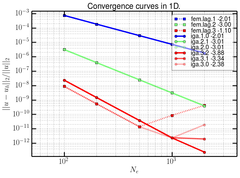
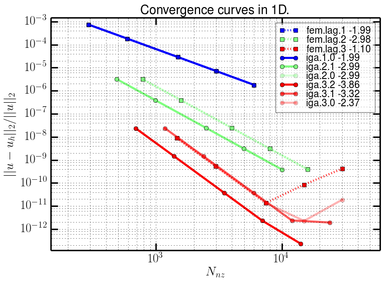
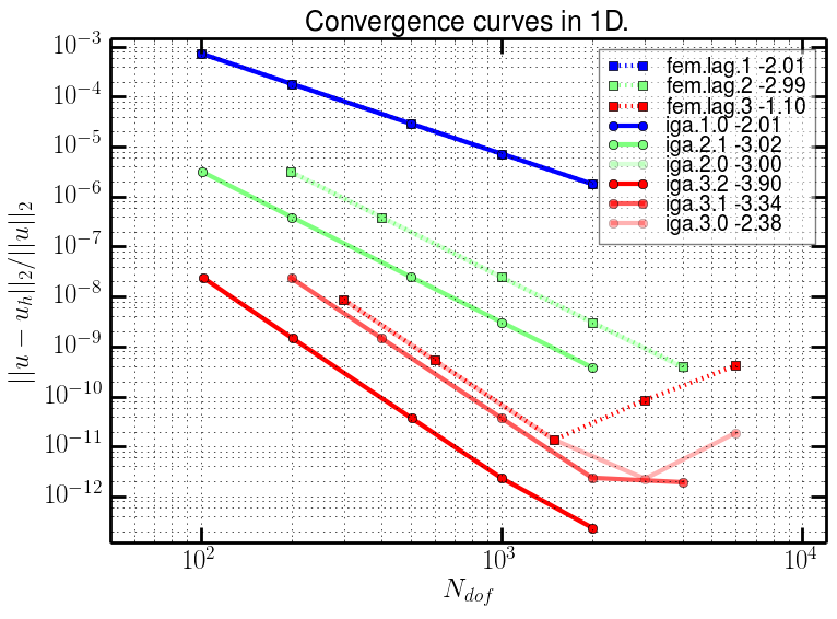
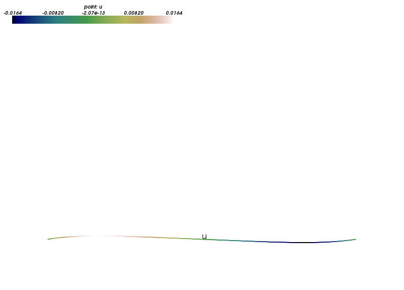
Figure 2: Convergence results for $u(x)\equiv\left(x^{4}-0.0625\right)\sin{\left(x\right)}$. The legend for the FEM shows the polynomial order and the slope of the corresponding curve. For the IGA it shows the degree, the global continuity, and the slope, respectively. The function $u$ is shown in bottom-right.

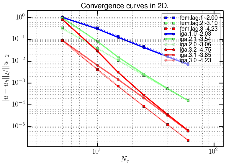
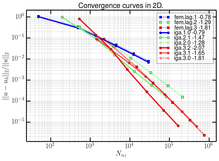
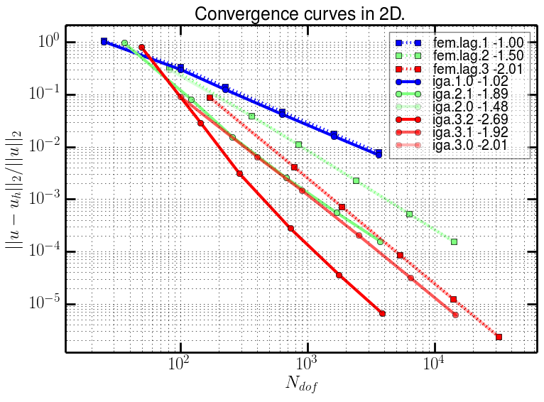
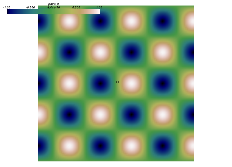
Figure 3: Convergence results for $u(x,y)\equiv\sin{\left(5\pi x\right)}\cos{\left(5\pi y\right)}$. The legend for the FEM shows the polynomial order and the slope of the corresponding curve. For the IGA it shows the degree, the global continuity, and the slope, respectively. The function $u$ is shown in bottom-right.

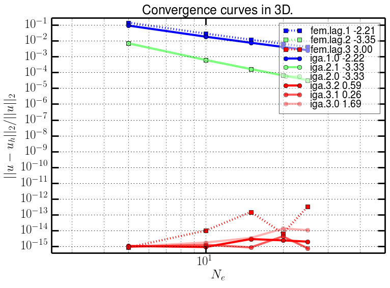
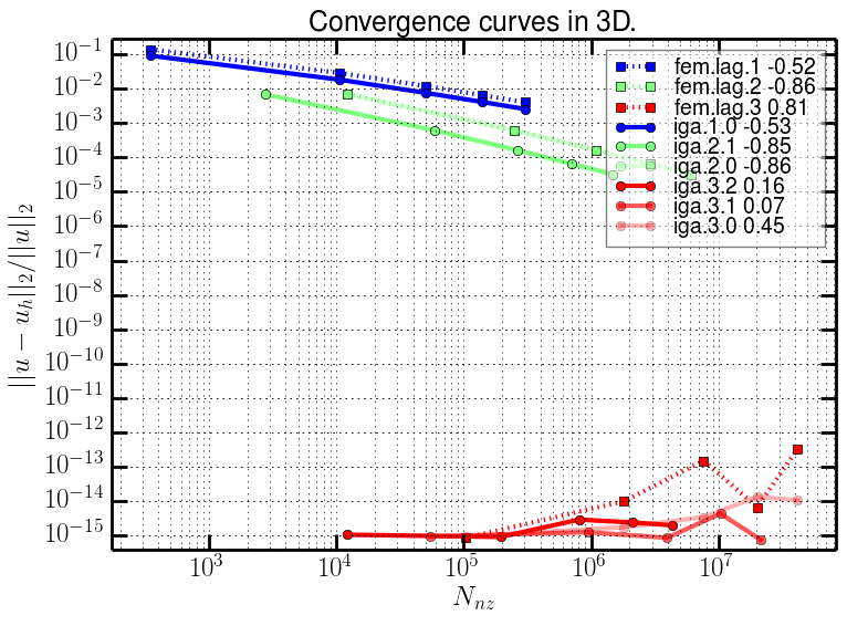
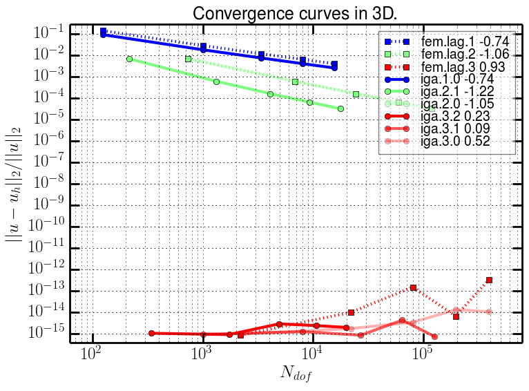
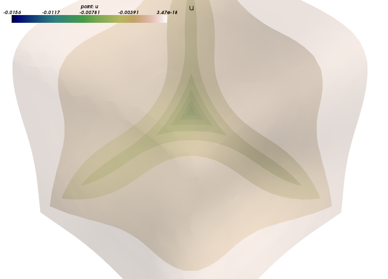
Figure 4: Convergence results for $u(x,y,z)\equiv\left(x^{3}-0.125\right)\left(y^{3}-0.125\right)\left(z^{3}-0.125\right)$. The legend for the FEM shows the polynomial order and the slope of the corresponding curve. For the IGA it shows the degree, the global continuity, and the slope, respectively. The function $u$ is shown in bottom-right.

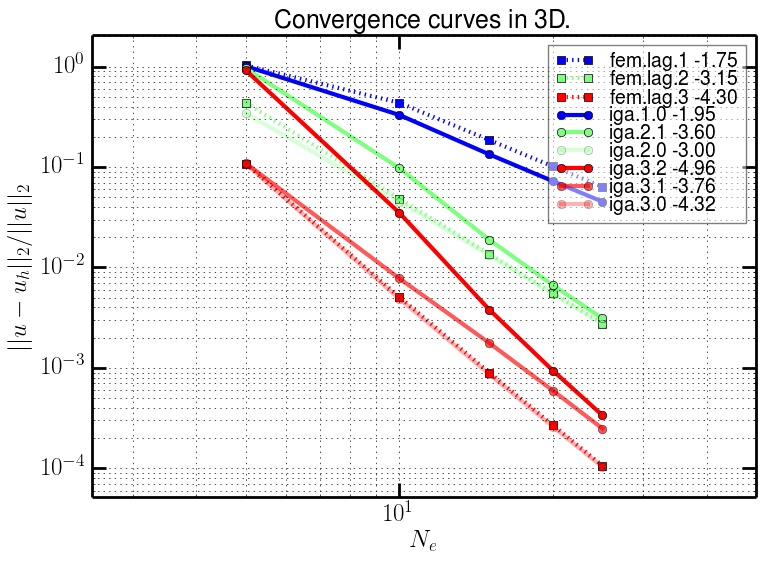
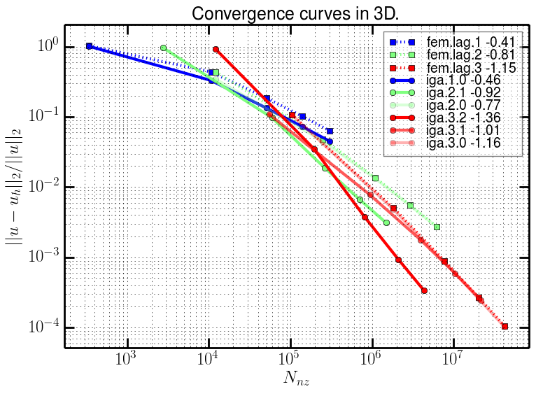
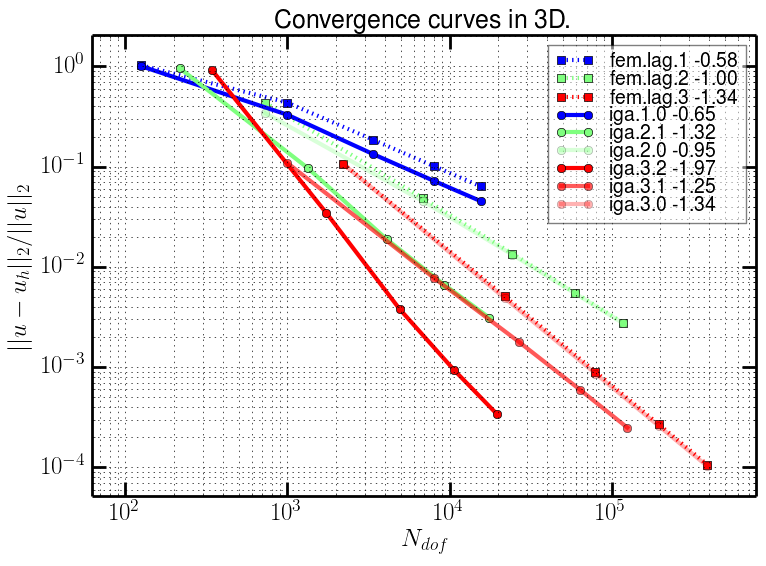
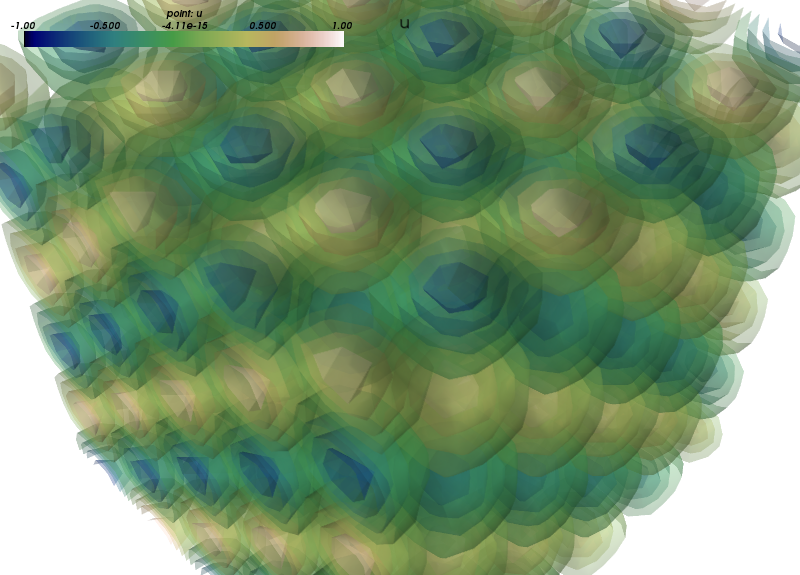
Figure 5: Convergence results for $u(x,y,z)\equiv\sin{\left(5\pi x\right)}\sin{\left(5\pi z\right)}\cos{\left(5\pi y\right)}$. The legend for the FEM shows the polynomial order and the slope of the corresponding curve. For the IGA it shows the degree, the global continuity, and the slope, respectively. The function $u$ is shown in bottom-right.

The convergence of FEM and IGA for the Poisson problem is compared in Figs. 2- 5. All the figures contain the convergence curves w.r.t. $N_{e}$ (top left), $N_{nz}$ (top right) and $N_{dof}$ (bottom left). The relative error $||u-u_{h}||_{2}/||u||_{2}$ is measured. The analytic solution $u$ is depicted in bottom right. The figure legends use the following naming scheme:

• FEM Lagrange basis: “fem.lag.$<$degree$>$ $<$slope$>$”;

• IGA basis: “iga.$<$degree$>$.$<$continuity$>$ $<$slope$>$”.

4.1.1 1D Poisson problem

In the 1D case (Fig. 2), $u(x)\equiv\left(x^{4}-0.0625\right)\sin{\left(x\right)}$ was used. Here, IGA with increasing continuity performs progressively better then FEM with the same polynomial order when the convergence w.r.t. $N_{nz}$ and $N_{dof}$ is considered. On the other hand, its error is slightly higher than the FEM or $C^{0}$ IGA error for the $N_{e}$ curve. The right parts of the curves for order/degree three solutions exhibit a loss numerical precision for very small errors — this loss of precision seems to decrease considerably with increasing the IGA basis continuity, and for the highest system resolution, IGA outperforms FEM even w.r.t. $N_{e}$. This is probably related to a better conditioning of the resulting linear system. Note that a direct solver [12] (version 5.6.2) was used in this case, so the solutions should be “exact” up to the machine precision.

4.1.2 2D Poisson problem

In the 2D case (Fig. 3), $u(x,y)\equiv\sin{\left(5\pi x\right)}\cos{\left(5\pi y\right)}$ was used. In terms of $N_{dof}$, similar results as in the 1D case were obtained, i.e., increasing the global continuity of the IGA basis improves the convergence in comparison with FEM. The same holds for $N_{nz}$ after a certain minimal system resolution. Also again as in 1D, the standard $C^{0}$ basis performs better when considering convergence w.r.t. $N_{e}$.

4.1.3 3D Poisson problems

In 3D, two solutions were considered. The first solution $u(x,y,z)\equiv\left(x^{3}-0.125\right)\left(y^{3}-0.125\right)\left(z^{3}-0.125\right)$ (Fig. 4) is a tensor product of order three polynomials. The results reflect that as a numerical “zero” error is obtained independently of the resolution for the order/degree three bases. The higher continuity of IGA seems again to mitigate a slight loss of precision for higher resolutions.

The second solution $u(x,y,z)\equiv\sin{\left(5\pi x\right)}\sin{\left(5\pi z\right)}\cos{\left(5\pi y\right)}$ (Fig. 5) is a direct generalization of the 2D case, and behaves in the same way.

The conjugate gradient iterative solver from PETSc [1], preconditioned by the incomplete Cholesky decomposition was used in the 2D and 3D cases. The absolute precision for preconditioned residuals was set to $10^{-18}$, so that “exact” solutions are obtained.

4.2 Simple eigenvalue problems

Several simple quantum mechanical systems were considered for our convergence study, namely an infinite potential well in 2D and 3D, a linear harmonic oscillator in 2D and 3D, and a hyperbolic 2D potential. The domain was a unit cube (or square): $\Omega\equiv[-a/2,a/2]^{d}$, $d=1,2,3$. The discretization parameters are summarized in Tab. 2. We were interested in convergence of the two smallest eigenvalues to the analytic values $\bar{\varepsilon}_{i}$. The error was measured using $\sum_{i=1,2}(|\varepsilon_{i}-\bar{\varepsilon}_{i}|)/2$.

system	dimension	$N_{e}$	edge length $a$
well	2D	20, 50, 100, 250	1
well	3D	5, 10, 20, 35	1
oscillator	2D	20, 50, 100, 250	10
oscillator	3D	5, 10, 20, 35	10
hyperbolic	2D	20, 50, 100, 250	30

Table 2: Simple eigenvalue problem: discretization parameters — numbers of vertices/knots along the domain edge and the domain edge length.

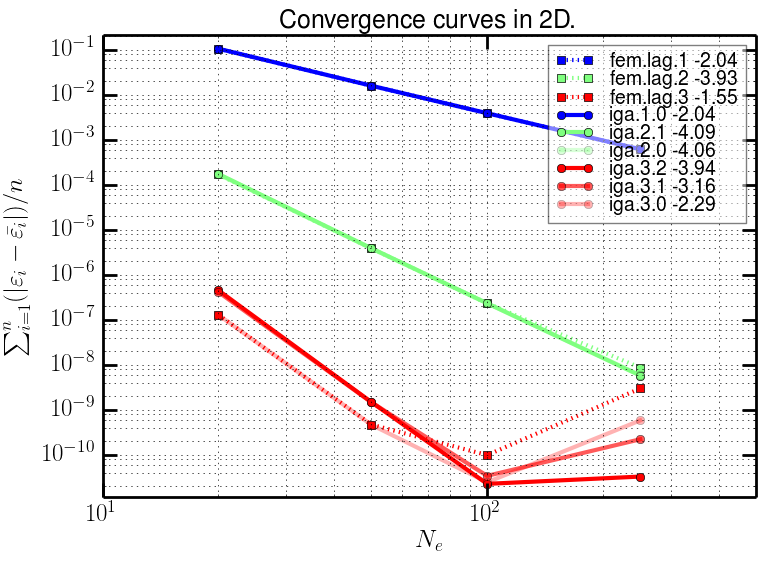
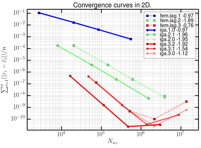
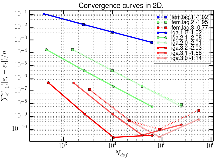
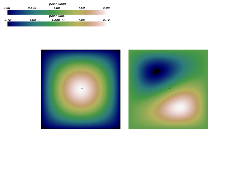
Figure 6: Convergence results for the 2D well eigenvalue problem. The legend for the FEM shows the polynomial order and the slope of the corresponding curve. For the IGA it shows the degree, the global continuity, and the slope, respectively. The eigen-functions are shown in bottom-right.

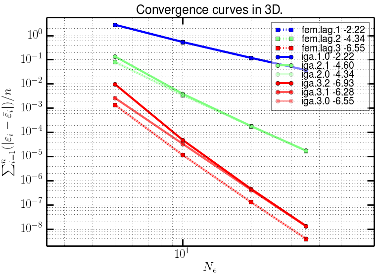
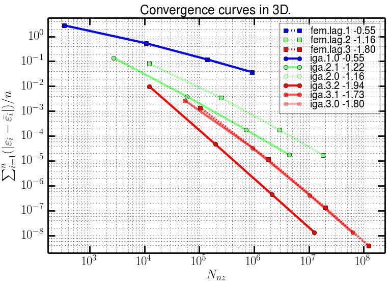
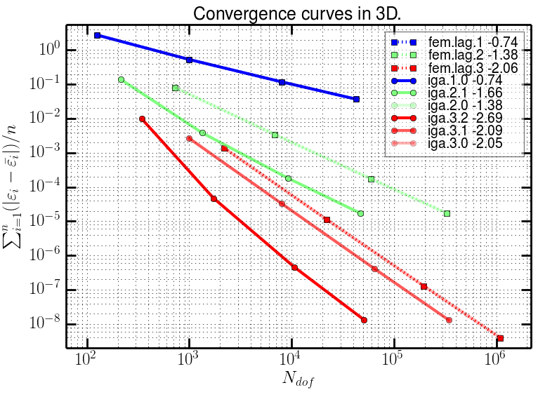
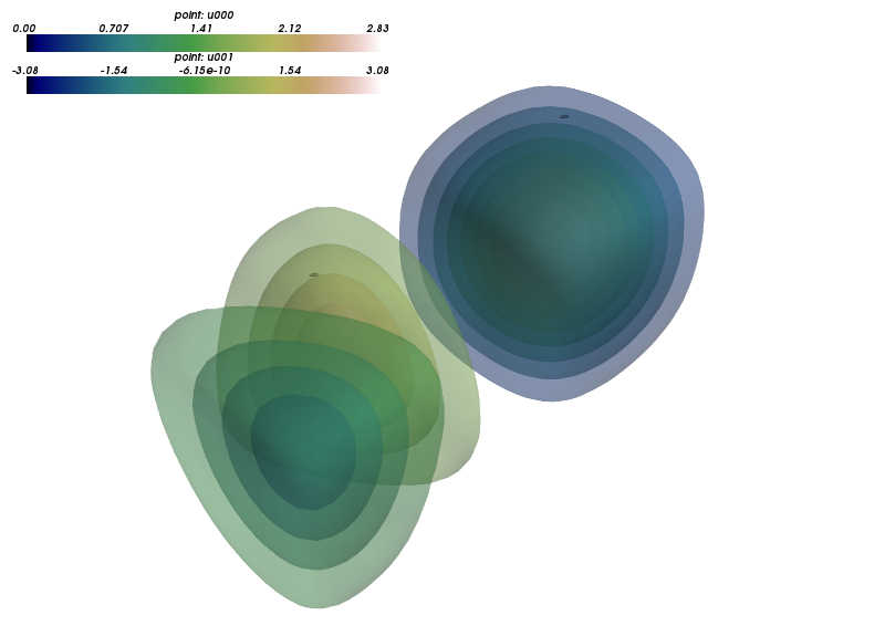
Figure 7: Convergence results for the 3D well eigenvalue problem. The legend for the FEM shows the polynomial order and the slope of the corresponding curve. For the IGA it shows the degree, the global continuity, and the slope, respectively. The eigen-functions are shown in bottom-right.

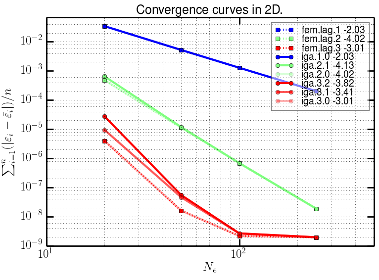
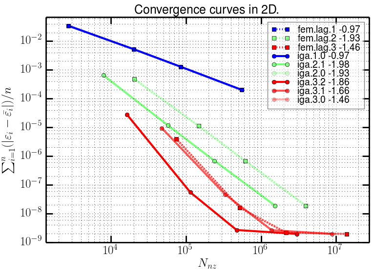
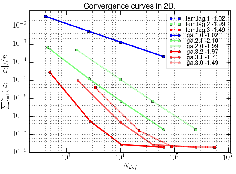
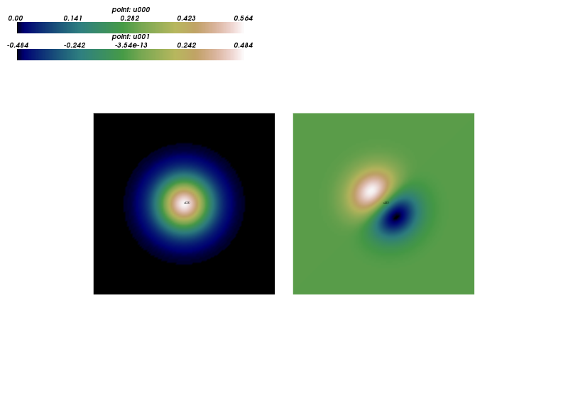
Figure 8: Convergence results for the 2D oscillator eigenvalue problem. The legend for the FEM shows the polynomial order and the slope of the corresponding curve. For the IGA it shows the degree, the global continuity, and the slope, respectively. The eigen-functions are shown in bottom-right.

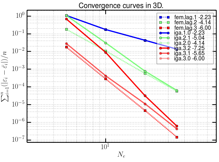
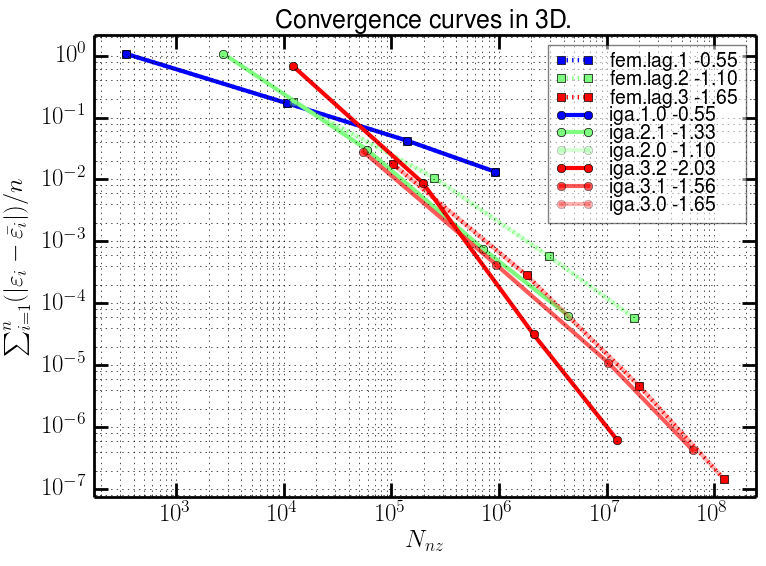
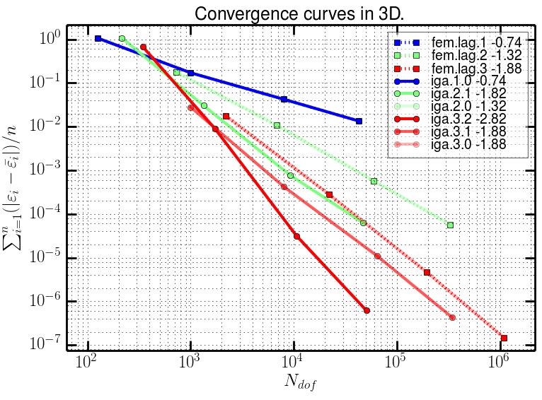
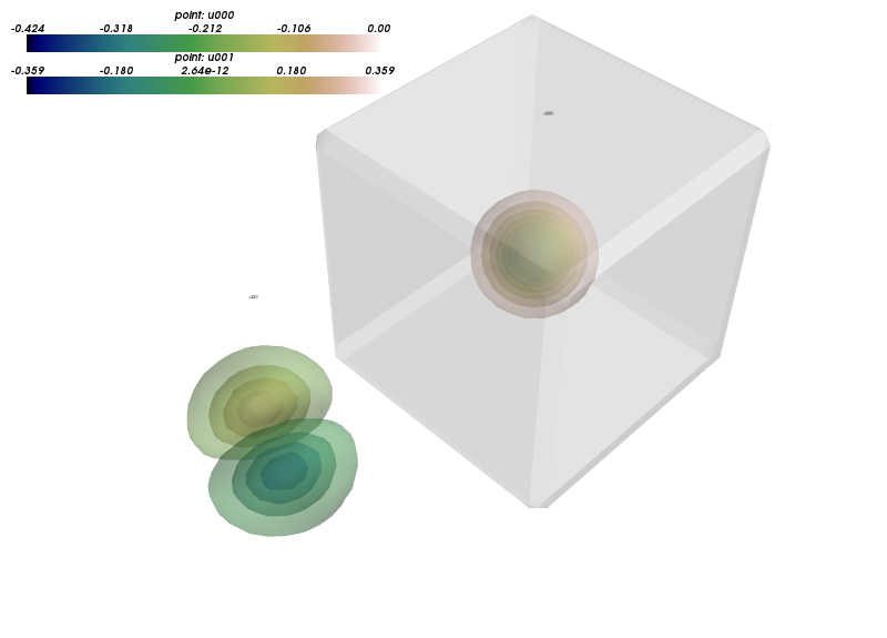
Figure 9: Convergence results for the 3D oscillator eigenvalue problem. The legend for the FEM shows the polynomial order and the slope of the corresponding curve. For the IGA it shows the degree, the global continuity, and the slope, respectively. The eigen-functions are shown in bottom-right.

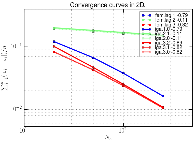
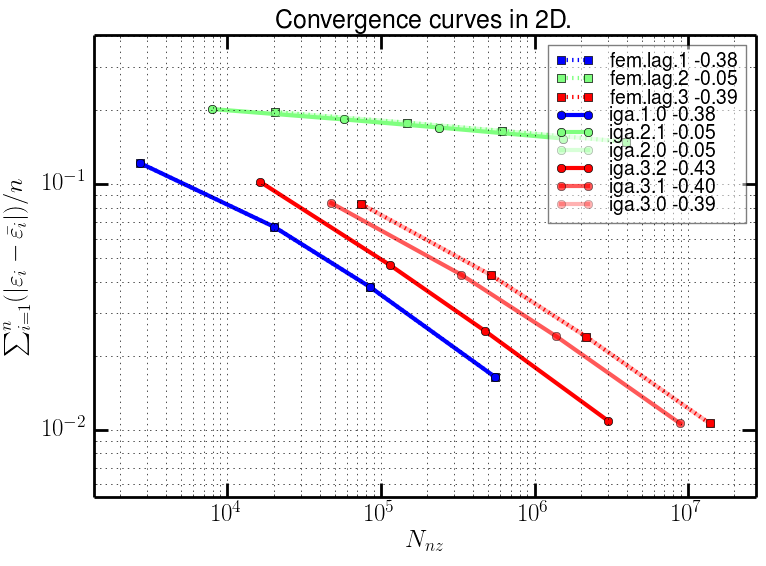
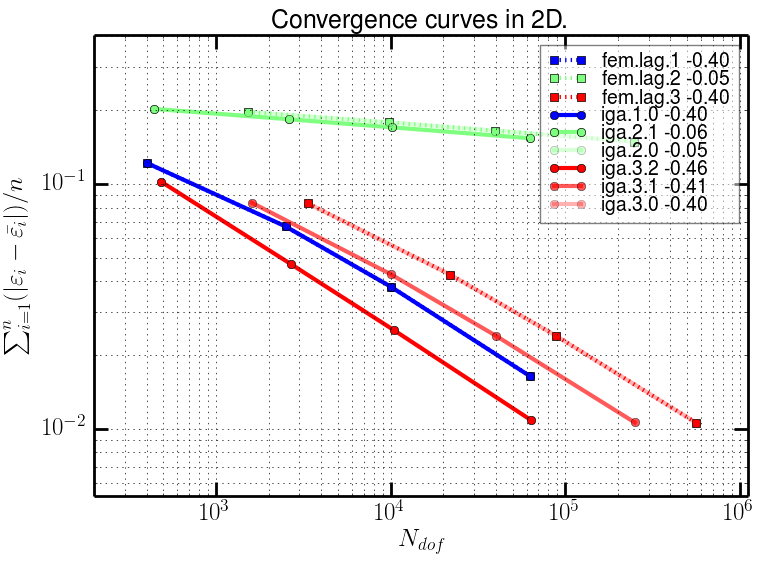
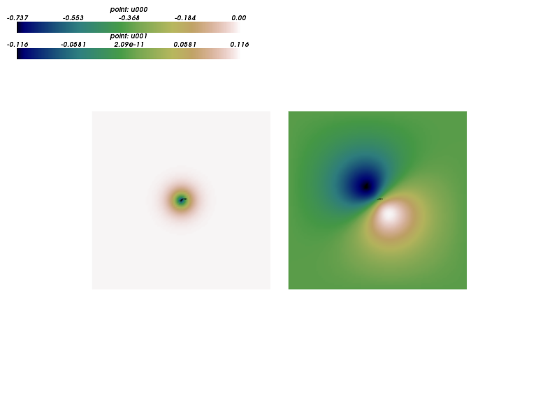
Figure 10: Convergence results for the 2D hyperbolic eigenvalue problem. The legend for the FEM shows the polynomial order and the slope of the corresponding curve. For the IGA it shows the degree, the global continuity, and the slope, respectively. The eigen-functions are shown in bottom-right.

The convergence of FEM and IGA for the simple eigenvalue problems is compared in Figs. 6- 10. All the figures contain the convergence curves w.r.t. $N_{e}$ (top left), $N_{nz}$ (top right) and $N_{dof}$ (bottom left). The eigen-functions corresponding to $\varepsilon_{1}$, $\varepsilon_{2}$ are depicted in bottom right. The figure legends use the same naming scheme as in 4.1. All eigenvalue problems in this section were solved using the JDSYM solver from Pysparse [16].

4.2.1 Infinite potential well

The potential well can be described by (15) with a trivial choice of the potential: $V(\bm{r})\equiv 0$. The exact eigenvalues are given by

$$\bar{\varepsilon}_{i}=\frac{\pi^{2}}{2a^{2}}c_{i}\mbox{ , where }c_{i}=\left\{\begin{array}[]{c}2,5\mbox{ in 2D,}\\ 3,6\mbox{ in 3D.}\end{array}\right.$$

In our case, $\bar{\varepsilon}_{i}$ was equal to 9.869604401089358, 24.674011002723397 in 2D and to 14.804406601634037, 29.608813203268074 in 3D.

The convergence curves for the 2D case are shown in Fig. 6. Here, IGA with increasing continuity performs progressively better then FEM with the same polynomial order when the convergence w.r.t. $N_{nz}$ and $N_{dof}$ is considered. On the other hand, its error is slightly higher than the FEM or $C^{0}$ IGA error for the $N_{e}$ curve. The right parts of the curves for order/degree three solutions exhibit a loss numerical precision for very small errors — this loss of precision seems to decrease with increasing the IGA basis continuity, and for the highest system resolution, IGA outperforms FEM even w.r.t. $N_{e}$. This is probably related to a better conditioning of the resulting eigenvalue problem. Compare to the 1D Poisson problem example in Section 4.1, where also the convergence to machine precision limits was achieved.

The convergence curves for the 3D case are shown in Fig. 7. The results are qualitatively analogous to the 2D case, but without the loss of numerical precision, because the machine precision limit was not reached.

4.2.2 Linear harmonic oscillator

The linear harmonic oscillator can be described by (15) with a particular choice of the potential: $V(\bm{r})\equiv\frac{1}{2}\bm{r}^{2}$. The exact eigenvalues $\bar{\varepsilon}_{i}$ are equal to 1, 2 in 2D and to 1.5, 2.5 in 3D.

The convergence curves for the 2D case are shown in Fig. 8 and are analogous to the 2D potential well results, with the exception that the higher continuity of IGA does not help to fight the machine precision limit.

The convergence curves for the 3D case are shown in Fig. 9 and qualitatively correspond to the 3D potential well results.

4.2.3 Hyperbolic 2D potential

The hyperbolic 2D potential serves as a non-physical 2D analogy of Coulombic potential for hydrogen atom. It can be described by (15) with a particular choice of the potential: $V(\bm{r})\equiv-\frac{1}{2\bm{r}}$. The exact eigenvalues $\bar{\varepsilon}_{i}$ are equal to -0.5, $-0.0\bar{5}$, according to

$$\bar{\varepsilon}_{i}=-\frac{1}{8(i-0.5)^{2}}\mbox{ , where }i=1,2\;.$$

Unlike the previous examples, the potential $V(\bm{r})$ has a singularity at $\bm{r}=0$. To avoid numerical problems, the singularity removed by setting the radii smaller than $10^{-6}$ to $10^{-6}$. Due to that, the numerical solutions converge to slightly different values than given above. Nevertheless, as can be seen in Fig. 10, the convergence of IGA solution with high global continuity seems to be better than that of FEM in terms of $N_{e}$ and $N_{dof}$, and worse in case of $N_{nz}$.

Note that the singularity problem is not present in full DFT scheme below, thanks to the use of carefully chosen pseudopotentials.

4.3 DFT loop

The computations were done on a cube domain having the edge size of 14 atomic units, with varying number of vertices/knots along an edge. A nitrogen atom was used for the benchmark due to availability of reference solution values for this simple system.

The tri-cubic FEM basis and degree three IGA basis were used. The continuities $C^{0}$, $C^{1}$ and $C^{2}$ were used for the IGA basis. In Fig. 11 we can see the convergence of the first eigenvalue $\varepsilon_{1}$ of problem (15) to a reference value. The Fig. 12 depicts the convergence of the charge density $\rho$ to a reference value.

The following observations can be made from both figures. As expected, the IGA with $C^{0}$ continuity is exactly equivalent to the FEM. The higher degree of continuity in IGA leads to an improved convergence w.r.t. $N_{nz}$ and $N_{dof}$, and a worse convergence w.r.t. $N_{e}$.

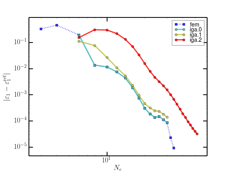
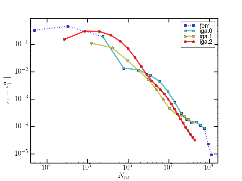
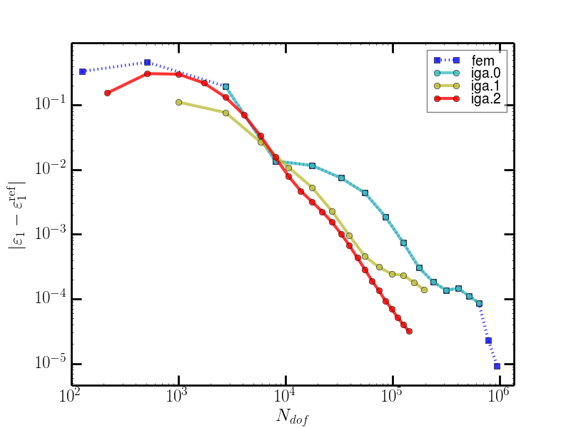
Figure 11: Convergence of the first eigenvalue $\varepsilon_{1}$: difference w.r.t. a reference value. The IGA labels indicate the global basis continuity.

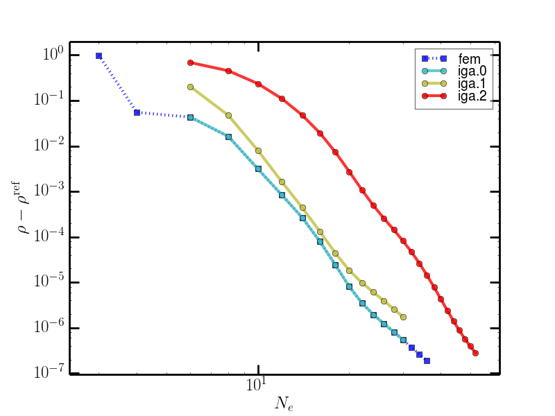
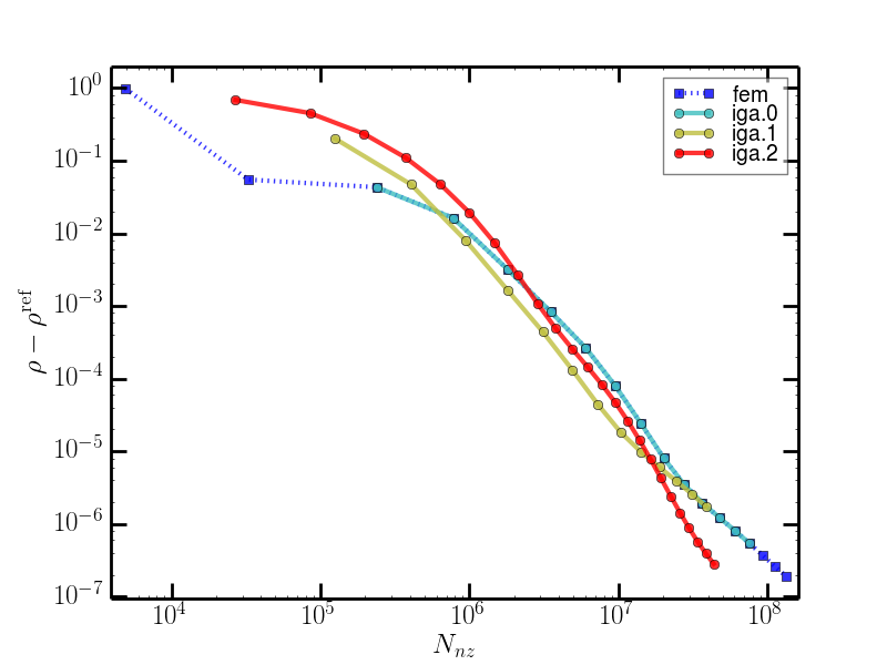
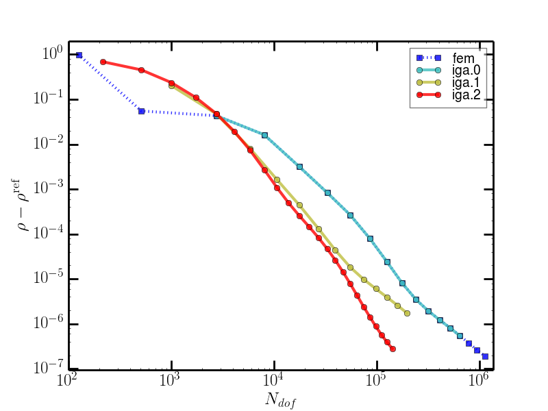
Figure 12: Convergence of the charge density $\rho$: difference w.r.t. a reference value. The IGA labels indicate the global basis continuity.

4.4 Results Summary

We were interested in convergence w.r.t. three parameters: the number of vertices/knots along the domain edge $N_{e}$ ($\approx$ cost of quadrature and assembling), the number of non-zero entries in the matrices $N_{nz}$ ($\approx$ cost of matrix-vector products) and the total number of degrees of freedom $N_{dof}$. The convergence of the Poisson equation solution to a manufactured analytical solution, the convergence of two smallest eigenvalues of simple quantum mechanical systems and finally the convergence of the complete DFT loop were assessed.

As reported in Section 4.1, in all tests, IGA with $C^{2}$ global continuity is the most efficient in term of convergence w.r.t. $N_{dof}$, i.e., the sizes of the vectors and matrices involved, which relate to the difficulty of solving the Poisson equation (16) or the eigenvalue problem (15).

In the Poisson equation test problems, IGA with increasing continuity performs progressively better then FEM with the same polynomial order when the convergence w.r.t. $N_{nz}$ and $N_{dof}$ is considered. On the other hand, the standard $C^{0}$ basis performs better when considering convergence w.r.t. $N_{e}$.

Similar results were obtained in eigenvalue problems in Section 4.2 originating from simple quantum mechanical systems. Again, IGA with increasing continuity performs progressively better then FEM with the same polynomial order considering convergence w.r.t. $N_{nz}$ and $N_{dof}$, and IGA error is slightly higher than FEM or $C^{0}$ IGA errors for the $N_{e}$ curves.

Considering the convergence of the eigenvalue $\varepsilon_{1}$ and the charge density $\rho$ computed by the complete DFT loop in Section 4.3, increasing the IGA basis continuity improves again the convergence w.r.t. $N_{nz}$ and $N_{dof}$. In the case of the convergence w.r.t. $N_{e}$, however, increasing the basis continuity (and thus decreasing $N_{dof}$ for the same number of elements) leads to a significantly worse convergence. This corresponds to a much higher numerical quadrature cost of $C^{2}$ IGA basis when compared to a $C^{0}$ basis of the same accuracy.

5 Conclusion

We compared numerical convergence properties of FEM and IGA using problems originating from various stages of our electronic structure calculation algorithm, based on the density functional theory, the environment-reflecting pseudopotentials and a weak solution of the Kohn-Sham equations. Our computer implementation built upon the open source package SfePy supports computations both with the FE basis and the NURBS or B-splines basis of IGA. The latter allows a high global continuity in approximation of unknown fields, so convergence properties of B-spline bases with global continuities up to $C^{2}$ were examined, because having a globally $C^{2}$ continuous approximation is crucial for efficient computing of derivatives of the total energy w.r.t. atomic positions etc., as given by the Hellmann-Feynman theorem [9].

Overall, the results summarized in Section 4.4 support our choice of IGA as a viable alternative to FEM in electronic structure calculations. To alleviate the numerical quadrature cost, reduced quadrature rules has been proposed for the context of the Bézier extraction [31], which we plan to assess in future.

Acknowledgments: The work was supported by the Grant Agency of the Czech Republic, project P108/11/0853. R. Kolman’s work was supported by the grant project of the Czech Science Foundation (GACR), No. GAP 101/12/2315, within the institutional support RVO:61388998.

References

References

-
[1]
S. Balay, S. Abhyankar, M. F. Adams, J. Brown, P. Brune, K. Buschelman,
L. Dalcin, V. Eijkhout, W. D. Gropp, D. Kaushik, M. G. Knepley, L. C.
McInnes, K. Rupp, B. F. Smith, S. Zampini, H. Zhang, PETSc users manual,
Tech. Rep. ANL-95/11 - Revision 3.6, Argonne National Laboratory (2015).
URL http://www.mcs.anl.gov/petsc - [2] Y. Bazilevs, V. M. Calo, J. A. Cottrell, J. A. Evans, T. J. R. Hughes, S. Lipton, M. A. Scott, T. W. Sederberg, Isogeometric analysis using T-splines, Comput. Methods Appl. Mech. Engrg. 199 (2010) 229–263.
- [3] Y. Bazilevs, L. B. a. da Veiga, J. A. Cottrell, T. J. R. Hughes, G. Sangalli, Isogeometric analysis: approximation, stability and error estimates for h-refined meshes, Math Models Methods Appl Sci 16 (2011) 1031–1090.
- [4] L. Beirão da Veiga, A. Buffa, J. Rivas, G. Sangalli, Some estimates for refinement in isogeometric analysis, Numerische Mathematik 118 (2) (2011) 271–305.
- [5] M. J. Borden, M. A. Scott, J. A. Evans, T. J. R. Hughes, Isogeometric finite element data structures based on Bezier extraction of NURBS, Int. J. Numer. Meth. Engng. 87 (2011) 15–47.
- [6] A. Buffa, G. Sangalli, C. Schwab, Exponential convergence of the hp version of isogeometric analysis in 1d, in: Spectral and High Order Methods for Partial Differential Equations - ICOSAHOM 2012, vol. 95 of Lecture Notes in Computational Science and Engineering, Springer International Publishing, 2014, pp. 191–203.
-
[7]
R. Cimrman, Enhancing SfePy with isogeometric analysis, in: P. de Buyl,
N. Varoquaux (eds.), Proceedings of the 7th European Conference on Python in
Science (EuroSciPy 2014), 2014, pp. 65–72.
URL http://arxiv.org/abs/1412.6407 -
[8]
R. Cimrman, SfePy - write your own FE application, in: P. de Buyl,
N. Varoquaux (eds.), Proceedings of the 6th European Conference on Python in
Science (EuroSciPy 2013), 2014, pp. 65–70.
URL http://arxiv.org/abs/1404.6391 - [9] R. Cimrman, M. Novák, R. Kolman, M. Tůma, J. Vackář, Isogeometric analysis in electronic structure calculations, Mathematics and Computers in Simulation n/a (n/a) (2015) n/a – n/a, submitted.
- [10] N. Collier, D. Pardo, L. Dalcin, M. Paszynski, V. M. Calo, The cost of continuity: A study of the performance of isogeometric finite elements using direct solvers, Computer Methods in Applied Mechanics and Engineering 213–216 (2012) 353 – 361.
- [11] J. A. Cottrell, T. J. R. Hughes, Y. Bazilevs, Isogeometric Analysis: Toward Integration of CAD and FEA, John Wiley & Sons, 2009.
- [12] T. A. Davis, Algorithm 832: UMFPACK v4.3—an unsymmetric-pattern multifrontal method, ACM Trans. Math. Softw. 30 (2) (2004) 196–199.
- [13] D. Davydov, T. D. Young, P. Steinmann, On the adaptive finite element analysis of the Kohn-Sham equations: Methods, algorithms, and implementation, International Journal for Numerical Methods in Engineering (2015) n/a–n/a.
- [14] A. Di Pomponio, A. Continenza, R. Podloucky, J. Vackář, Symmetrization of atomic forces within the full-potential linearized augmented-plane-wave method, Phys. Rev. B 53 (1996) 9505–9508.
- [15] R. M. Dreizler, E. K. U. Gross, Density Functional Theory, Springer-Verlag, 1990.
-
[16]
R. Geus, D. Wheeler, D. Orban, Pysparse documentation.
URL http://pysparse.sourceforge.net - [17] T. J. R. Hughes, The Finite Element Method: Linear Static and Dynamic Finite Element Analysis, Dover Publications, 2000.
- [18] J. Ihm, A. Zunger, C. M. L., Momentum-space formalism for the total energy of solids, J. Phys. C: Solid State Phys. 12 (1979) 4409–4422.
- [19] W. Kohn, L. J. Sham, Self-consistent equations including exchange and correlation effects, Phys. Rev. 140 (4A) (1965) A1133–A1138.
- [20] R. Kolman, J. Plešek, M. Okrouhlík, Complex wavenumber Fourier analysis of the B-spline based finite element method, Wave Motion 51 (2013) 348–359.
- [21] R. Kolman, S. V. Sorokin, B. Bastl, J. Kopačka, J. Plešek, Isogeometric analysis of free vibration of simple shaped elastic samples, Journal of the Acoustical Society of America 137 (4) (2015) 2089–2100.
- [22] M. Kästner, P. Metsch, R. de Borst, Isogeometric analysis of the Cahn–Hilliard equation – a convergence study, Journal of Computational Physics (2015) –.
- [23] R. M. Martin, Electronic Structure: Basic Theory and Practical Methods, Cambridge University Press, 2005.
- [24] A. Masud, R. Kannan, B-splines and {NURBS} based finite element methods for Kohn–Sham equations, Computer Methods in Applied Mechanics and Engineering 241–244 (2012) 112–127.
- [25] P. Motamarri, V. Gavini, Subquadratic-scaling subspace projection method for large-scale Kohn-Sham density functional theory calculations using spectral finite-element discretization, Phys. Rev. B 90 (2014) 115127.
- [26] P. Motamarri, M. R. Nowak, K. Leiter, J. Knap, V. Gavini, Higher-order adaptive finite-element methods for Kohn–Sham density functional theory, Journal of Computational Physics 253 (2013) 308–343.
- [27] R. G. Parr, Y. Weitao, Density-Functional Theory of Atoms and Molecules, Oxford University Press, USA, 1994.
- [28] W. E. Pickett, Pseudopotential methods in condensed matter applications, Comp. Phys. Reports 9 (1989) 115–198.
- [29] L. Piegl, W. Tiller, The NURBS Book, (2nd ed.) ed., Springer-Verlag, 1995-1997.
- [30] D. Schillinger, J. A. Evans, A. Reali, M. A. Scott, T. J. R. Hughes, Isogeometric collocation: Cost comparison with Galerkin methods and extension to adaptive hierarchical {NURBS} discretizations, Computer Methods in Applied Mechanics and Engineering 267 (2013) 170 – 232.
- [31] D. Schillinger, S. J. Hossain, T. J. R. Hughes, Reduced Bézier element quadrature rules for quadratic and cubic splines in isogeometric analysis, Computer Methods in Applied Mechanics and Engineering 277 (2014) 1–45.
- [32] G. Strang, G. Fix, An Analysis of the Finite Element Method, Wellesley-Cambridge Press, Wellesley, 2008, pp. 414.
- [33] J. Vackář, A. Šimunek, Adaptability and accuracy of all-electron pseudopotentials, Phys. Rev. B 67, 125113.
- [34] J. Vackář, O. Čertík, R. Cimrman, M. Novák, O. Šipr, J. Plešek, Advances in the Theory of Quantum Systems in Chemistry and Physics, vol. 22 of Prog. Theoretical Chem. and Phys., chap. Finite Element Method in Density Functional Theory Electronic Structure Calculations, Springer, 2011, pp. 199–217.
- [35] M. Weinert, J. W. Davenport, Fractional occupations and density-functional energies and forces, Phys. Rev. B 45 (1992) 13709–13712.
- [36] R. Yu, D. Singh, H. Krakauer, All-electron and pseudopotential force calculations using the linearized-augmented-plane-wave method, Phys. Rev. B 43 (1991) 6411–6422.