Optimal tuning of a confined Brownian information engine

Abstract

A Brownian information engine is a device extracting a mechanical work from a single heat bath by exploiting the information on the state of a Brownian particle immersed in the bath. As for engines, it is important to find the optimal operating condition that yields the maximum extracted work or power. The optimal condition for a Brownian information engine with a finite cycle time $\tau$ has been rarely studied because of the difficulty in finding the nonequilibrium steady state. In this study, we introduce a model for the Brownian information engine and develop an analytic formalism for its steady state distribution for any $\tau$. We find that the extracted work per engine cycle is maximum when $\tau$ approaches infinity, while the power is maximum when $\tau$ approaches zero.

I Introduction

The information engine refers to a system extracting a work from a single heat bath by using the information on the microscopic state of the system. Discussions on the information engine date back to the thought experiment on Maxwell’s Demon suggested in 1871 Leff and Rex (2003). Through the thought experiment, Maxwell claimed that the entropy can be decreased apparently by performing measurements and feedback controls on a thermodynamic system. Later on, Szilard Szilard (1929) proposed a primary model for the information engine. In this model he showed that a work can be extracted from a single heat bath, the entropy of which decreases. These examples had been regarded as a paradox because the thermodynamic second law prohibits the total entropy from decreasing. However, in 2009, Sagawa et al. Sagawa and Ueda (2009) resolved this paradox by discovering the information fluctuation theorems  Sagawa and Ueda (2009, 2010); they showed that the thermodynamic entropy (work) can be decreased (extracted) as much as the mutual information gain by the measurement. After this discovery, there has been a surge of interest in studying the information fluctuation theorems Ponmurugan (2010); Horowitz and Vaikuntanathan (2010); Sagawa (2011); Vaikuntanathan and Jarzynski (2011); Sagawa and Ueda (2012, 2012); Lahiri et al. (2012); Hartich et al. (2014) and developing theoretical models for the information engine from classical Mandal and Jarzynski (2012); Barato and Seifert (2012); Horowitz and Parrondo (2011); Bergli (2014); Pal et al. (2014); Abreu and Seifert (2011, 2012); Mandal et al. (2013); Bauer et al. (2012); Kosugi (2013) to quantum Kim et al. (2011) systems. With the help of technological advancement, several information engines have been realized in electronic Koski et al. (2014, 2014) and Brownian systems Lopez et al. (2008); Toyabe et al. (2010).

Among many examples, Brownian systems are a good test base for the classical stochastic theory based on the Langevin or Fokker-Plank equations. For this reason, many researchers have studied the information engines consisting of a Brownian particles trapped in a harmonic potential Pal et al. (2014); Abreu and Seifert (2011); Bauer et al. (2012); Kosugi (2013). For example, Abreu et al. Abreu and Seifert (2011) studied the case where the potential center is varied, Bauer et al. Bauer et al. (2012) studied the case where the potential center and the stiffness are varied, and Kosugi Kosugi (2013) investigated a similar problem.

In a practical aspect, the primary concern for the Brownian information engine lies in the efficiency. More specifically, we are interested in two quantities: The extracted work per engine cycle and the extracted work per unit time, i.e., the power. In a classical heat engine without exploiting any information, the maximum efficiency is achieved when the engine is operated quasi-statically and reversibly. However, the power vanishes in a reversible engine and the condition for the maximum power is different from that for the maximum efficiency Curzon and Ahlborn (1975). In this work, we investigate the optimal condition for the extracted work per engine cycle or the power in a model for the Brownian information engine.

In spite of its practical importance, the optimal tuning of the Brownian information engine has been studied rarely due to the difficulty in finding the nonequilibrium steady state of an engine having finite engine cycle time $\tau$. The optimal tuning conditions have been studied mostly for engines with $\tau=\infty$ Abreu and Seifert (2011). Kosugi Kosugi (2013) developed a formalism for finite $\tau$, but only the infinite $\tau$ limit was addressed.

In this study, we introduce a model for the information engine consisting of a Brownian particle confined in a harmonic potential. In this model, one engine cycle of duration $\tau$ consists of the three processes: measurement of the particle position, feedback control of the potential center, and relaxation. We derive a self-consistent equation for the steady state probability distribution function for general $\tau$, whose solution is found in a series expansion form. Using this formalism, we obtain the optimal parameters set that yields the maximum extracted work per cycle and the maximum power. We find that the global maximum of the extracted work per cycle is realized when $\tau$ is taken to be infinity. On the other hand, the global maximum of the power is achieved in the $\tau\to 0$ limit.

This paper is organized as follows. In Sec. II, we introduce our model. In Sec. III, we develop a formalism for the nonequilibrium steady state distribution of the system. Using the formalism, we investigate the optimal condition for the maximum work per cycle and the power in Sec. IV. We conclude the paper with summary in Sec. V.

II Description of the Model

We consider a one-dimensional overdamped Langevin dynamics of a Brownian particle in a heat bath with temperature $T$. The particle is confined by an external harmonic potential $V(X,\lambda(t))=\frac{1}{2}k(X-\lambda(t))^{2}$ where $X$ is the position of the Brownian particle, $k$ is a stiffness constant, and $\lambda(t)$ denotes a time-dependent potential center with $\lambda(0)=0$. This dynamics is described by the Langevin equation

$$\gamma\frac{dX}{dt}=-k(X-\lambda(t))+\xi(t),$$ (1)

where $\gamma$ is the damping coefficient, and $\xi\left(t\right)$ is a Gaussian white noise satisfying $\left<\xi\left(t\right)\right>=0$ and $\left<\xi\left(t\right)\xi\left(t^{\prime}\right)\right>=2{\gamma k_{B}T}\delta\left(t-t^{\prime}\right)$ with the Boltzmann constant $k_{B}$. The bracket $\left<\cdots\right>$ means the ensemble average. Note that the Langevin dynamics (1), when $\lambda(t)$ is time-independent, is known as the Ornstein-Uhlenbeck process Gardiner (2010); Risken (1989). For convenience, we will set $\gamma=k=k_{B}T=1$.

The Brownian system can be used as an information engine by measuring $X$ and controlling $\lambda(t)$ depending on the measurement outcome. Here, we consider the following time-periodic measurement and the feedback control operations, which are also illustrated in Fig. 1.

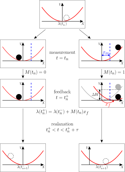
Figure 1: (Color online) Illustration of the engine cycle during the time interval $t_{n}\leq t<t_{n+1}$ of the engine. At the measurement step, it is determined whether the particle is on the left hand side ($M(t_{n})=0$) or right hand side ($M(t_{n})=1$) of the position $\lambda(t_{n}^{-})+x_{m}$ represented by the (blue) dashed line. At the feedback step, if $M\left(t_{n}\right)=1$, the potential center is instantaneously shifted to $\lambda(t_{n}^{+})=\lambda(t_{n}^{-})+x_{f}$ and the mechanical work $\Delta W(t_{n})$ is extracted. At the relaxation step, the particle is relaxed with the fixed potential center at $\lambda(t_{n}^{+})$ until the next cycle starts at time $t_{n+1}$.

Measurement – At time $t=n\tau\equiv t_{n}$ $(n=0,1,2,...)$, a measurement is performed to determine which side of a reference position at $\lambda(t_{n})+x_{m}$ the Brownian particle is located at. The measurement outcome is represented by a binary parameter

$$M(t_{n})=\left\{\begin{array}[]{cl}1&\mbox{ if }X(t_{n})\geq\lambda(t_{n})+x_{m},\\[5.69054pt] 0&\mbox{ if }X(t_{n})<\lambda(t_{n})+x_{m}.\end{array}\right.$$ (2)

The information obtained during the measurement step can be exploited to extract a work.

Feedback control – When $M_{n}(t_{n})=0$, the potential center remains unchanged. That is,

$$\lambda(t_{n}^{+})=\lambda(t_{n}^{-}),$$ (3)

where $t_{n}^{-}~{}(t_{n}^{+})$ denotes the moment just before (after) the measurement performed at time $t_{n}$. On the other hand, when $M(t_{n})=1$, the potential center is shifted instantaneously by the amount of $x_{f}$:

$$\lambda(t_{n}^{+})=\lambda(t_{n}^{-})+x_{f}.$$ (4)

By shifting the potential center, we can extract a work $\Delta W(t_{n})$ as much as the change in the potential energy caused by the shift. We adopt a convention that $\Delta W(t_{n})$ is positive (negative) when the work is produced by (done on) the Brownian particle. It is given by

$$\begin{split}\Delta W(t_{n})&=V\left(X(t_{n}),\lambda(t_{n}^{-})\right)-V\left(X(t_{n}),\lambda(t_{n}^{+})\right)\\ &=x_{f}\left(X(t_{n})-\lambda(t_{n}^{-})-\frac{1}{2}x_{f}\right).\end{split}$$ (5)

Note that the extracted work is negative when $x_{f}<0$. Hence, we only consider the case with $x_{f}\geq 0$.

Relaxation – In the time interval $t_{n}<t<t_{n+1}$, the particle evolves in time with fixed $\lambda(t)=\lambda(t_{n}^{+})$ according to the Langevin equation (1) until the next cycle begins at time $t_{n+1}$. During this step, the particle exchanges the thermal energy with the heat bath.

The engine is characterized by the three parameters: $x_{m}$ for the measurement, $x_{f}$ for the feedback, and $\tau$ for the relaxation. Thus, the extracted work per cycle or the power depends on the choice of those parameters. We are interested in the optimal choice of the parameters under which the steady state average of the extracted work per cycle or the power becomes maximum. We remark that our model is a generalized version of the information ratchet introduced in Ref. Sagawa and Ueda (2010), which corresponds to the case with $x_{f}=2x_{m}$ and $\tau=\infty$.

III Coordinate transformation

The engine configuration is specified by the positions of the particle $X$ and the potential center $\lambda$. Note that the potential center is shifted by the amount of $x_{f}$ each time the measurement outcome is 1. Hence, it is convenient to introduce an integer variable $l\equiv\lambda/x_{f}$ which counts the number of potential-center shifts. We introduce $P_{n}(X,l)$ to denote the joint probability distribution of $X$ and $l$ at time $t=t_{n}^{-}$. The joint probability distribution satisfies the recursion relation

$$\begin{split}P_{n+1}\left(X,l\right)&=\int_{-\infty}^{lx_{f}+x_{m}}K_{lx_{f}}^{\left(\tau\right)}\left(X|Z\right)P_{n}\left(Z,l\right)dZ\\ &+\int_{(l-1)x_{f}+x_{m}}^{\infty}K_{lx_{f}}^{\left(\tau\right)}\left(X|Z\right)P_{n}\left(Z,l-1\right)dZ,\end{split}$$ (6)

where

$$K_{\alpha}^{(\tau)}(X|Z)=\frac{\exp\left[-\frac{(X-\alpha-(Z-\alpha)e^{-\tau})^{2}}{2(1-e^{-2\tau})}\right]}{\sqrt{2\pi(1-e^{-2\tau})}}$$ (7)

is the transition probability of the Brownian particle from position $Z$ at time $0$ to position $X$ at time $\tau$ with the potential center being fixed at position $\alpha$. Note that this is the transition probability for the Ornstein-Uhlenbeck process Gardiner (2010); Risken (1989). The first (second) term on the right hand side of Eq. (6) accounts for the relaxation process after the feedback control corresponding to the measurement outcome $M(t_{n})=0~{}(1)$.

The extracted work is determined only by the relative position of the Brownian particle from the potential center. Hence, it is useful to change the variables from $(X,l)$ to $(x\equiv X-lx_{f},l)$. Then, by using the translational invariance $K_{\alpha}^{(\tau)}(x+\alpha|z+\alpha)=K_{0}^{(\tau)}(x|z)$, we can rewrite (6) as

$$\begin{split}P_{n+1}\left(x+lx_{f},l\right)=\int_{-\infty}^{x_{m}}K_{0}^{\left(\tau\right)}\left(x|z\right)P_{n}\left(z+lx_{f},l\right)dz\\ +\int_{x_{m}}^{\infty}K_{0}^{\left(\tau\right)}\left(x|z-x_{f}\right)P_{n}\left(z+(l-1)x_{f},l-1\right)dz.\end{split}$$ (8)

By summing Eq. (8) over all $l$, we obtain

$$\begin{split}p_{n+1}\left(x\right)&=\int_{-\infty}^{x_{m}}K_{0}^{\left(\tau\right)}\left(x|z\right)p_{n}\left(z\right)dz\\ &+\int_{x_{m}}^{\infty}K_{0}^{\left(\tau\right)}\left(x|z-x_{f}\right)p_{n}\left(z\right)dz,\end{split}$$ (9)

where

$$p_{n}\left(x\right)\equiv\sum_{l}P_{n}\left(x+lx_{f},l\right).$$ (10)

is the probability distribution function for the relative position $x$ at time $t_{n}^{-}$. This recursion relation can be understood in terms of an effective dynamics. In the effective dynamics, the potential center is fixed at the origin. Instead, the Brown particle is instantaneously shifted by the amount of $(-x_{f})$ when the measurement outcome is $M=1$. This effective dynamics is illustrated in Fig. 2 and will be referred to as the ‘fixed potential-center dynamics’.

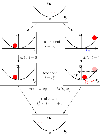
Figure 2: (Color online) Illustration for the engine cycle in the fixed potential-center dynamics. In contrast to the original dynamics, the particle is transported instantaneously by the amount of $-x_{f}$ with the potential center being fixed in the feedback process.

In the $n\rightarrow\infty$ limit, $p_{n}(x)$ will converge to the steady-state distribution $p_{ss}(x)$, which is given by the solution of the self-consistent equation

$$\begin{split}p_{ss}\left(x\right)&=\int_{-\infty}^{x_{m}}K_{0}^{\left(\tau\right)}\left(x|z\right)p_{ss}\left(z\right)dz\\ &+\int_{x_{m}}^{\infty}K_{0}^{\left(\tau\right)}\left(x|z-x_{f}\right)p_{ss}\left(z\right)dz.\end{split}$$ (11)

From Eq. (5), the work is extracted only when $x>x_{m}$ by the amount of $\Delta W=x_{f}(x-x_{f}/2)$ each cycle. Hence, the average extracted work per cycle in the steady state is given by

$$\langle\Delta W\rangle_{ss}=x_{f}\int_{x_{m}}^{\infty}\left(x-\frac{1}{2}x_{f}\right)p_{ss}(x)dx,$$ (12)

where $\langle\cdots\rangle_{ss}$ denotes the steady-state ensemble average. The integration in Eq. (12) begins at $x_{m}$ because the work can be extracted only when the particle position is larger than $x_{m}$ ($M=1$). Such an event occurs with the probability $P_{M}$ given by

$$P_{M}\equiv\int_{x_{m}}^{\infty}\ p_{ss}(x)dx\ .$$ (13)

Using this quantity, we can write $\langle\Delta W\rangle_{ss}$ as

$$\langle\Delta W\rangle_{ss}=x_{f}\left(\langle x\rangle_{M}-\frac{1}{2}x_{f}\right)P_{M},$$ (14)

where

$$\langle x\rangle_{M}\equiv\frac{1}{P_{M}}\int_{x_{m}}^{\infty}x\ {p_{ss}(x)}dx$$ (15)

is the mean position of the particle in the steady state given that $x\geq x_{m}$. The system acts as an engine with positive $\langle\Delta W\rangle_{ss}$ when

$$0<x_{f}<2\langle x\rangle_{M}\ .$$ (16)

IV Optimal condition for the engine

In this section, we develop an analytic formalism for $p_{ss}(x)$ and discuss the optimal operating condition for the engine. We address the special cases in the limit $\tau\to\infty$ and $\tau\to 0$, then proceed to the general case with nonzero and finite $\tau$.

IV.1 $\tau\rightarrow\infty$ case

When $\tau$ is infinite, the system relaxes to the equilibrium state irrespective of the measurement and the feedback control. Thus, the system follows the equilibrium distribution

$$p_{ss}(x)=\frac{1}{\sqrt{2\pi}}e^{-\frac{1}{2}x^{2}}.$$ (17)

It is easy to check that the equilibrium distribution is indeed the solution of the self-consistent equation (11) with $K_{0}^{\infty}(x|z)=e^{-x^{2}/2}/\sqrt{2\pi}$. Using this $p_{ss}(x)$, we obtain that

$$P_{M}=\frac{1}{2}\operatorname{erfc}\left(\frac{x_{m}}{\sqrt{2}}\right)\mbox{ and }\langle x\rangle_{M}=\sqrt{\frac{2}{\pi}}\frac{e^{-\frac{1}{2}x_{m}^{2}}}{\operatorname{erfc}\left(\frac{x_{m}}{\sqrt{2}}\right)}$$ (18)

where $\operatorname{erfc}(x)=\frac{2}{\sqrt{\pi}}\int_{x}^{\infty}e^{-y^{2}}dy$ is the complementary error function.

The optimal values of $x_{f}$ and $x_{m}$ at which the engine extracts the maximum amount of works are denoted by $x_{f}^{*}$ and $x_{m}^{*}$, respectively. They are obtained from the conditions $\partial\langle\Delta W\rangle_{ss}/\partial x_{f}|_{x_{f}=x_{f}^{*},x_{m}=x_{m}^{*}}=0$ and $\partial\langle\Delta W\rangle_{ss}/\partial x_{m}|_{x_{f}=x_{f}^{*},x_{m}=x_{m}^{*}}=0$, which yield that

$$x_{f}^{*} = \langle x\rangle_{M}|_{x_{m}=x_{m}^{*}},$$ (19)

$$x_{m}^{*} = \frac{x_{f}^{*}}{2}.$$ (20)

The former equation (19) for $x_{f}^{*}$ has a clear meaning: Given a particle position $x>x_{m}$, the work is extracted maximally by shifting the Brownian particle to the potential center (in the fixed potential-center dynamics). Thus, $x_{f}^{*}$ should be taken as the mean position of the particle under the condition that $M=1$. With the optimal choice of $x_{f}$, the mean value of the extracted work is given by $\langle\Delta W\rangle_{ss}=\frac{1}{2}\langle x\rangle_{M}^{2}P_{M}$. Note that $\frac{1}{2}\langle x\rangle_{M}^{2}$ is an increasing function of $x_{m}$ while $P_{M}$ is a decreasing function of $x_{m}$ (see (18)). Due to these competing effects, the work becomes maximum at a nontrivial value of $x_{m}^{*}$. Combining (19) and (20), one obtains the transcendental equation for $x_{m}^{*}$:

$$x_{m}^{*}=\frac{1}{\sqrt{2\pi}}\frac{e^{-\frac{1}{2}x_{m}^{*}}}{\operatorname{erfc}(x_{m}^{*}/\sqrt{2})}.$$ (21)

It has the numerical solution $x_{m}^{*}\simeq 0.612$. Therefore, $x_{f}^{*}=2x_{m}^{*}\simeq 1.224$ and the maximum average work per cycle $\left<\Delta W\right>_{ss}^{*}$ is given by

$$\left<\Delta W\right>_{ss}^{*}=\left.\frac{1}{2}\langle x\rangle_{M}^{2}P_{M}\right|_{x_{m}=x_{m}^{*}}\simeq 0.202.$$ (22)

Figure 3(a) shows the density plot of the average extracted work per cycle in the $(x_{m},x_{f})$ plane. The work is indeed maximum at $(0.612,1.224)$. We add a remark that the average power $\langle\Delta W\rangle_{ss}^{*}$ is zero because $\left<\Delta W\right>_{ss}^{*}$ is finite but $\tau\rightarrow\infty$.

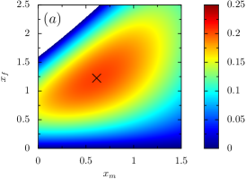
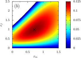
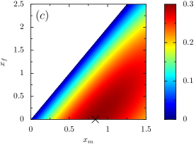
Figure 3: (Color online) (a) Density plot for $\langle\Delta W\rangle_{ss}$ in $\tau\rightarrow\infty$ limit. (b) Density plot for $\langle\Delta W\rangle_{ss}$ obtained from the truncation method when $L=4$ and $\tau=\log 2$. (c) Density plot for $w_{ss}$ in $\tau\rightarrow 0$ limit. The $times$ symbols represent the optimal position where the extracted work or the power is maximum.

IV.2 $\tau\rightarrow 0$ case

In the $\tau\rightarrow 0$ limit, the particle position is measured incessantly. Therefore, in the fixed potential-center dynamics, the particle is immediately shifted from $x_{m}$ to $x_{r}\equiv x_{m}-x_{f}$ whenever it touches the reference position $x_{m}$. This dynamics is similar to the resetting process studied by Evans and Majumdar Evans and Majumdar (2011). They investigated a search problem by a random walker whose position is reset to the origin at a constant rate. Along the similar line of reasoning, our resetting process can be described by the following Fokker-Planck equation:

$$\frac{\partial p(x,t)}{\partial t}=-\frac{\partial j(x,t)}{\partial x}+j_{r}(t)\delta(x-x_{r})$$ (23)

where $p(x,t)$ is the probability distribution of the particle in the fixed potential-center dynamics,

$$j(x,t)=\left(-x-\frac{\partial}{\partial x}\right)p(x,t)$$ (24)

is the probability current at position $x$ and at time $t$, and $j_{r}(t)=\lim_{x\to x_{m}^{-}}j(x,t)$ is the resetting current which is absorbed at $x_{m}$ and then injected at $x_{r}$. The probability distribution satisfies the absorbing boundary condition at $x_{m}$, i.e., $p(x=x_{m},t)=0$.

The steady-state probability distribution satisfies

$$-xp_{ss}(x)-\frac{\partial p_{ss}(x)}{\partial x}=\begin{cases}0&\mbox{for }x<x_{r}\\ j_{ss}&\mbox{for }x_{r}\leq x<x_{m}\\ 0&\mbox{for }x\geq x_{m}\end{cases}$$ (25)

where the steady-state resetting current is given by

$$j_{ss}=\lim_{t\to\infty}j_{r}(t)=-\left.\frac{\partial p_{ss}(x)}{\partial x}\right|_{x=x_{m}^{-}}.$$ (26)

Given $j_{ss}$, the solution satisfying the absorbing boundary condition is given by

$$p_{ss}\left(x\right)=\begin{cases}j_{ss}\int_{x_{r}}^{x_{m}}e^{\frac{1}{2}(z^{2}-x^{2})}dz&\mbox{for }x<x_{r},\\ j_{ss}\int_{x}^{x_{m}}e^{\frac{1}{2}(z^{2}-x^{2})}dz&\mbox{for }x_{r}\leq x<x_{m},\\ 0&\mbox{for }x\geq x_{m}.\end{cases}$$ (27)

The resetting current is determined by the normalization condition $\int p_{ss}(x)dx=1$. It is given by

$$\begin{split}j_{ss}=&\left[\left(\int_{-\infty}^{x_{r}}e^{-\frac{1}{2}x^{2}}dx\right)\left(\int_{x_{r}}^{x_{m}}e^{\frac{1}{2}z^{2}}dz\right)\right.\\ &+\left.\int_{x_{r}}^{x_{m}}\left(e^{-\frac{1}{2}x^{2}}\int_{x}^{x_{m}}e^{\frac{1}{2}z^{2}}dz\right)dx\right]^{-1}\end{split}$$ (28)

with $x_{r}=x_{m}-x_{f}$.

In the $\tau\to 0$ limit, the average extracted work per cycle vanishes because it takes infinitely many cycles for the Brownian particle to reach $x_{m}$ after a resetting. Thus, it is useful to consider the average power in the steady state $w_{ss}\equiv\lim_{\tau\to 0}\langle\Delta W\rangle_{ss}/\tau$. It is given by

$$w_{ss}=x_{f}\left(x_{m}-\frac{1}{2}x_{f}\right)j_{ss},$$ (29)

where $x_{f}(x_{m}-x_{f}/2)=V(x_{m},0)-V(x_{m}-x_{f},0)$ is the extracted work per resetting. Figure 3(c) shows the density plot for $w_{ss}$ in the $\tau\to 0$ limit in the $(x_{m},x_{f})$ plane.

The power is maximized when $\partial w_{ss}/\partial x_{m}=0$ and $\partial w_{ss}/\partial x_{f}=0$ simultaneously. A straightforward calculation shows that both conditions become identical when $x_{f}=0$, which implies that $x_{f}^{*}=0$. In the limit $x_{f}\to x_{f}^{*}=0$, the power becomes $w_{ss}=\sqrt{\frac{2}{\pi}}x_{m}e^{-x_{m}^{2}/2}/(1+\text{erf}(x_{m}/\sqrt{2}))$ with the error function ${\rm erf}(x)=1-{\rm erfc}(x)$. It takes the maximum value

$$w_{ss}^{*}\simeq 0.295~{}\textrm{at }x_{m}^{*}\simeq 0.840\textrm{ and }x_{f}^{*}=0.$$ (30)

Strictly speaking, the engine does not produce any work at $x_{f}=0$. The result $x_{f}^{*}=0$ should be understood as the limit $x_{f}\to 0^{+}$. In this limit, $V(x_{m},0)-V(x_{m}-x_{f},0)$, the work extracted in a feedback process, vanishes as $\mathcal{O}(x_{f})$, but the resetting current $j_{ss}$ in (28) diverges as $\mathcal{O}(x_{f}^{-1})$, which results in a finite power.

IV.3 Finite $\tau$ case

For finite $\tau$, $p_{ss}(x)$ cannot be obtained in a closed form. Thus, we try to find it in a series form

$$p_{ss}(x)=\sum_{n=0}^{\infty}c_{n}\phi_{n}(x)$$ (31)

using the basis functions $\phi_{n}(x)\equiv H_{n}\left(x/\sqrt{2}\right)e^{-\frac{1}{2}x^{2}}$ where $H_{n}\left(x\right)$ is the Hermite polynomial of degree $n$ Arfken and Weber (1995). The Hermite polynomials satisfy the orthogonality condition

$$\int_{-\infty}^{\infty}H_{n}\left(\frac{x}{\sqrt{2}}\right)H_{l}\left(\frac{x}{\sqrt{2}}\right)e^{-\frac{1}{2}x^{2}}dx=N_{n}{\delta_{nl}}$$ (32)

with $N_{n}\equiv\sqrt{2\pi}2^{n}n!$. The expansion coefficients are represented by a column vector $\bm{c}=(c_{0},c_{1},c_{2},\ldots)^{T}$ where the superscript ^T stands for the transpose. The normalization condition $\int p_{ss}(x)dx=1$ fixes $c_{0}=1/\sqrt{2\pi}$. The other coefficients will be determined by using the self-consistent equation (11).

Such an expansion (31) is natural because $\phi_{n}(x)$ is the eigenfunction of the Fokker-Planck operator $\mathcal{L}(x)=\frac{\partial}{\partial x}\left(x+\frac{\partial}{\partial x}\right)$ for the Ornstein-Uhlenbeck process Risken (1989), i.e.,

$$\mathcal{L}(x)\phi_{n}(x)=-n\phi_{n}(x).$$ (33)

The transition probability $K_{0}^{(\tau)}(x|z)$ in Eq. (11) can be written in terms of $\mathcal{L}(x)$ as $K_{0}^{(\tau)}(x|z)=e^{\tau\mathcal{L}(x)}\delta(x-z)$. Thus, Eq. (11) can be rewritten as

$$p_{ss}\left(x\right)=e^{\tau\mathcal{L}(x)}\left[p_{ss}^{0}(x)+p_{ss}^{1}(x+x_{f})\right],$$ (34)

where $p_{ss}^{0}(x)\equiv\Theta(x_{m}-x)p_{ss}(x)$ and $p_{ss}^{1}(x)\equiv\Theta(x-x_{m})p_{ss}(x)=p_{ss}(x)-p_{ss}^{0}(x)$ with the Heaviside step function $\Theta(x)$.

Our strategy is to expand both sides of (34) using the basis set $\{\phi_{n}\}$. First of all, the function $p_{ss}^{0}(x)+p_{ss}^{1}(x+x_{f})$ in the right hand is expanded as

$$p_{ss}^{0}(x)+p_{ss}^{1}(x+x_{f})=\sum_{n=0}^{\infty}c^{\prime}_{n}\phi_{n}(x).$$ (35)

The expansion coefficients $\bm{c}^{\prime}=(c_{0}^{\prime},c_{1}^{\prime},\cdots)^{T}$ are obtained by integrating both sides of (35) after being multiplied with $H_{m}(x/\sqrt{2})$. One obtains that

$$\bm{c}^{\prime}=(\mathsf{A}+\mathsf{B})\bm{c},$$ (36)

where the matrix elements of $\mathsf{A}$ and $\mathsf{B}$ are defined as

$$A_{nl} = \frac{1}{N_{n}}\int_{-\infty}^{x_{m}}H_{n}\left(\frac{x}{\sqrt{2}}\right)\phi_{l}(x)dx,$$ (37)

$$B_{nl} = \frac{1}{N_{n}}\int_{x_{m}}^{\infty}H_{n}\left(\frac{x-x_{f}}{\sqrt{2}}\right)\phi_{l}(x)dx.$$ (38)

Note that the Hermite polynomials satisfy the identity

$$H_{n}(x+y)=H_{n}(x)+\sum_{k=0}^{n-1}\binom{n}{k}(2y)^{n-k}H_{k}(x),$$ (39)

with the binomial coefficient $\binom{n}{k}$. This identity allows us to rewrite A+B as

$$\mathsf{A+B}=\mathsf{I+F},$$ (40)

where $\mathsf{I}$ is the identity matrix and $\mathsf{F}$ has the elements

$$F_{nl}=\frac{1}{N_{n}}\sum_{k=0}^{n-1}\binom{n}{k}\left(-\sqrt{2}x_{f}\right)^{n-k}\int_{x_{m}}^{\infty}H_{k}\left(\frac{x}{\sqrt{2}}\right)\phi_{l}(x)dx$$

for $n\geq 1$ and $F_{nl}=0$ for $n=0$. Using $e^{\tau\mathcal{L}(x)}\phi_{n}(x)=e^{-n\tau}\phi_{n}(x)$ and introducing a diagonal matrix W with elements $W_{nl}=e^{-n\tau}\delta_{nl}$, we finally obtain the self-consistent equation

$$\bm{c}=\mathsf{W}(\mathsf{I+F})\bm{c}.$$ (41)

It is more convenient to work with

$$\bm{d}=\mathsf{W}^{-1}\bm{c},$$ (42)

with which the self-consistent equation (41) becomes

$$\bm{d}=(\mathsf{I+F})\mathsf{W}\bm{d}.$$ (43)

The average extracted work per cycle is given by

$$\begin{split}\langle\Delta W\rangle_{ss}=&\int_{x_{m}}^{\infty}\left(\frac{1}{2}x^{2}-\frac{1}{2}(x-x_{f})^{2}\right)p_{ss}(x)dx\\ =&\int_{-\infty}^{\infty}\frac{1}{2}x^{2}\left(p_{ss}^{1}(x)-p_{ss}^{1}(x+x_{f})\right)dx.\end{split}$$ (44)

The involved distribution functions are expanded as $(p_{ss}^{1}(x)-p_{ss}^{1}(x+x_{f}))=-\sum_{n}(\mathsf{F}\bm{c})_{n}\phi_{n}(x)$ using (35), (36), and (40). Note that $x^{2}=H_{2}(x/\sqrt{2})/2+H_{0}(x/\sqrt{2})$. Hence, using the orthogonality (32) of the Hermite polynomials, we obtain that

$$\langle\Delta W\rangle_{ss}=-\sqrt{8\pi}(\mathsf{F}\bm{c})_{2}=-\sqrt{8\pi}\left(1-e^{-2\tau}\right)d_{2}\ .$$ (45)

For the second equality, $\mathsf{F}\bm{c}=(\mathsf{W}^{-1}-\mathsf{I})\bm{c}=(\mathsf{I}-\mathsf{W})\bm{d}$ is used.

The formal solution of $\bm{d}$ is easily derived. First, we write $\bm{d}$, $\mathsf{W}$, and $\mathsf{F}$ in a block form as

$$\bm{d}=(d_{0},\tilde{\bm{d}})^{T},\ \mathsf{W}=\left(\begin{array}[]{cc}1&0\\ 0&\widetilde{\mathsf{W}}\end{array}\right)\mbox{, and }\mathsf{F}=\left(\begin{array}[]{cc}0&0\\ \tilde{\bm{f}}&\widetilde{\mathsf{F}}\end{array}\right),$$ (46)

and define the column vectors $\tilde{\bm{d}}=(d_{1},d_{2},\cdots)^{T}$ with $d_{n}=e^{n\tau}c_{n}$ and $\tilde{\bm{f}}=(f_{1},f_{2},\cdots)^{T}$ with $f_{n}=F_{n0}$, and matrices $\widetilde{\mathsf{W}}$ and $\widetilde{\mathsf{F}}$ accordingly. Inserting these block forms into (43), we obtain the formal solution for $\tilde{\bm{d}}$ as

$$\tilde{\bm{d}}=c_{0}\left[\mathsf{I}-(\mathsf{I}+\widetilde{\mathsf{F}})\widetilde{\mathsf{W}}\right]^{-1}\tilde{\bm{f}}$$ (47)

with $c_{0}=1/\sqrt{2\pi}$. It is crucial to have the formal solution that the first row of $\mathsf{F}$ vanishes ($F_{0n}=0$).

The formal solution involves an inversion of infinite-dimensional matrices, hence a closed-form expression is not available. Nevertheless, it is useful because it enables us to obtain an approximate solution systematically. First, we truncate the matrices $\widetilde{\mathsf{F}}$ and $\widetilde{\mathsf{W}}$ to $L\times L$ matrices $\widetilde{\mathsf{F}}^{(L)}$ and $\widetilde{\mathsf{W}}^{(L)}$ and the vector $\widetilde{\bm{f}}$ to an $L\times 1$ vector $\tilde{\bm{f}}^{(L)}$, respectively, i.e., $\widetilde{F}^{(L)}_{nm}=\widetilde{F}_{nm}$, $\widetilde{W}^{(L)}_{nm}=\widetilde{W}_{nm}$, and $\tilde{f}^{(L)}_{n}=\tilde{f}_{n}$ for $n,m=1,2,\dots,L$. They are inserted into (47) to yield a truncated solution $\tilde{\bm{d}}^{(L)}$. We note that $\widetilde{\mathsf{F}}$ and $\tilde{\bm{f}}$ depend on $x_{m}$ and $x_{f}$ but not on $\tau$, while the diagonal matrix $\widetilde{\mathsf{W}}$ depends only on $\epsilon\equiv e^{-\tau}\leq 1$. Therefore, the truncated solution $\tilde{\bm{d}}^{(L)}$ is the exact up to $\mathcal{O}(\epsilon^{L})$. Then, from Eq. (45), we can obtain the approximate solution for the average extracted work $\langle\Delta W\rangle_{ss}^{(L)}=-\sqrt{8\pi}\left(1-e^{-2\tau}\right)\tilde{d}_{2}^{(L)}$, which is also exact up to $\mathcal{O}(\epsilon^{L})$.

Figure 3(b) shows the density plot for $\langle\Delta W\rangle_{ss}^{(L)}$ with $L=4$ and at $\tau=\ln 2$. It is maximum at the point $(x_{m}^{*},x_{f}^{*})$ marked by the symbol $\times$ whose position can be found numerically. In Fig. 4, we present the traces of $(x_{m}^{*},x_{f}^{*})$ as $\tau$ is varying with $L=2,4,6,8$. Along each line, $x_{m}^{*}~{}(x_{f}^{*})$ decreases (increases) as $\tau$ increases. The lines converge to a single curve at large values of $\tau$. The convergence becomes poor in the region of small $\tau$ where the truncation parameter $\epsilon=e^{-\tau}$ is not small.

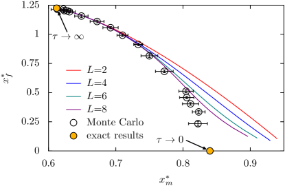
Figure 4: Parametric plot for the optimal control parameters $(x_{m}^{*}(\tau),x_{f}^{*}(\tau))$. The solid lines are obtained from the truncation method for $L=2,4,6,8$. The results obtained from the Monte Carlo simulations are denoted by open circles with error bars. The exact results in $\tau\rightarrow 0$ and $\tau\rightarrow\infty$ are marked by arrows.

We also performed the Monte Carlo simulations to obtain the optimal parameter values. In the Monte Carlo simulations, the Langevin equation (1) was integrated numerically over $10^{9}$ engine cycles to estimate the average extracted work in the steady state. In order to estimate $x_{m}^{*}$ and $x_{f}^{*}$, we discretized $x_{m}$ and $x_{f}$ in units of $\Delta x_{m}=\Delta x_{f}=0.01$. Among the grid points of $(x_{m},x_{f})$, we selected nine points having the largest values of $\langle\Delta W\rangle_{ss}$. Their averages were taken as the the Monte Carlo results and the standard deviations as the error bars for $x_{m}^{*}$, $x_{f}^{*}$, and $\langle\Delta W\rangle_{ss}^{*}$. The simulated $x_{m}^{*}$ and $x_{f}^{*}$ are plotted with open symbols in Fig. 4 with error bars. The exact optimal values in the $\tau\rightarrow 0$ and $\tau\rightarrow\infty$ limits are also plotted in Fig. 4 with closed symbols for comparison. As seen in the figure, our simulated data at large and small $\tau$ are close to the exact results in $\tau\rightarrow\infty$ and $\tau\rightarrow 0$, respectively, which supports the validity of our Monte Carlo simulations. The analytic results are in good agreement with the Monte Carlo results unless $\tau$ is too small.

Figure 5 presents the plot of $\langle\Delta W\rangle_{ss}^{*}$ as a function of $\epsilon=e^{-\tau}$. As the figure shows, the Monte Carlo results (open symbols) and the analytic results (lines) agree perfectly well even for small values of $L$. The numerical results show that $\langle\Delta W\rangle_{ss}^{*}$ increases as $\tau$ increases so that the global maximum of $\langle\Delta W\rangle_{ss}^{*}$ is attained when $\tau\rightarrow\infty$. Note the extracted work from an information engine is bounded by the change in the mutual information between the engine and the measurement outcome during the relaxation process Sagawa and Ueda (2010, 2012). When $\tau\rightarrow\infty$, the mutual information generated at the measurement step completely vanishes during the relaxation step. This might be the reason why the average extracted work is maximum at $\tau\rightarrow\infty$.

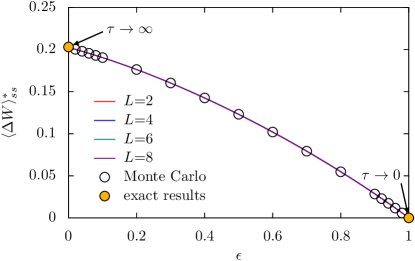
Figure 5: Parametric plot for the optimal work per cycle $\langle\Delta W\rangle_{ss}^{*}$. Results obtained from the truncation method are denoted by solid lines. Open circles present the Monte Carlo simulations results. The exact results in $\tau\rightarrow 0$ and $\tau\rightarrow\infty$ are marked by arrows.

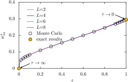
Figure 6: Parametric plot for the optimal power $w_{ss}^{*}$. Results obtained from the truncation method are denoted by solid lines. Open circles present the Monte Carlo simulations results. The exact results in $\tau\rightarrow 0$ and $\tau\rightarrow\infty$ are marked by arrows.

Figure 6 shows the optimal power $w_{ss}^{*}=\langle\Delta W\rangle_{ss}^{*}/\tau$ as a function of $\epsilon$. In contrast to the optimal work $\langle\Delta W\rangle_{ss}^{*}$ per cycle, the optimal power $w_{ss}^{*}$ is a decreasing function of $\tau$ and becomes maximum in the limiting case $\tau\to 0$. This indicates that the continuous time operation is the best way to achieve the maximum power of the Brownian information engine. Our model assumes that measurement and feedback processes do not cost any energy. If they cost some energy, the global maximum of the power will be realized at finite $\tau$.

V Conclusion

We studied the information engine where the Brownian particle is confined in a harmonic potential. This engine consists of the three processes: measurement of the particle position, instantaneous shift of the potential center depending on the measurement outcome, and relaxation of the particle. Each process is characterized by the model parameter: $x_{m}$ for the measurement, $x_{f}$ for the feedback, and $\tau$ for the relaxation. Using the coordinate transformation, we derived the self-consistent equation for the steady state distribution function of the particle in the fixed potential-center dynamics. The average work extracted out of the information engine per cycle is found from the steady state distribution.

When $\tau\rightarrow\infty$, the steady state becomes the equilibrium state. When $\tau\to 0$, the dynamics becomes similar to the resetting process Evans and Majumdar (2011) and the exact steady state distribution is obtained by analyzing the corresponding Fokker-Planck equation. When $\tau$ is finite, the steady-state distribution has the infinite series expansion in terms of the Hermite polynomials, which can be approximated systematically by truncating the infinite series. We show that the extracted work per cycle is maximum at $\tau=\infty$ and the the extracted power is maximum in the limiting case $\tau\to 0$.

A Brownian particle confined by a harmonic potential is realized by the optical trap experiment as in e.g. Ref. Lee et al. (2015). We expect that our theoretical model can be tested in such experiments. In our model, the Brownian particle exhibits a ballistic motion as the engine operates. This suggests that one can design an information motor which rectifies the thermal fluctuations with the help of measurement and feedback controls. Further studies along this direction would be interesting.