New perturbative method for analytical solutions in single-field models of inflation

Abstract

We propose a new parametrization of the background equations of motion corresponding to (canonical) single-field models of inflation, which allows a better understanding of the general properties of the solutions and of the corresponding predictions in the inflationary observables. Based on the tools of dynamical systems, the method suggests that inflation comes in two flavors: power-law and de Sitter. Power-law inflation seems to occur for a restricted type of potentials, whereas de Sitter inflation has a much broader applicability. We also show a general perturbative method, by means of series expansion, to solve the new equations of motion around the critical point of the de Sitter type, and how the method can be used for arbitrary models of de Sitter inflation. It is then argued that for the latter there are two general classes of inflationary solutions, given in terms of the behavior of the tensor-to-scalar ratio as a function of the number $N$ of $e$-folds before the end of inflation: $r\sim N^{-1}$ (Class I), or $r\sim N^{-2}$ (Class II). We give some examples of the two classes in terms of known scalar field potentials, and compare their general predictions with constraints obtained from observations.

I Introduction

Inflation remains one of the cornerstones of modern cosmology, and it still has a prominent place within the big bang model for the evolution of the Universe. According to recent accounts from the cosmic microwave background (CMB) measurements by the Planck Collaboration, single-field models of inflation are still among the best candidates to explain the features of the primordial power spectrum of density perturbationsAde et al. (2015).

Large efforts have been dedicated to solving the equations of motion of inflationary scalar fields under different techniques, and one of the most successful of them is the well-known slow-roll approximationLiddle and Lyth (2000); *Mukhanov:2005sc. The two basic assumptions for slow roll are that the energy density is dominated by the scalar potential, and that the scalar field itself is evolving slowly enough to guarantee an extended period of accelerated expansion. The equations of motion for the background can then be written in a closed form that allows general solutions, up to quadratures, of the scalar field as a function of the number of $e$-foldings of expansion for any scalar potential. The background solution is then used to calculate different features of the linear field perturbations that can be compared with actual observations. Although the general solution of the field perturbations is the same for any scalar field model of inflation, the final output depends on the specific background evolution, and it is because of this that observations may potentially distinguish among different inflationary modelsMalik and Wands (2009).

It is then necessary to have a good understanding of the background evolution for different models if one is to find the one preferred by the observations. Even though good numerical resources are now at handMortonson et al. (2011), the thorough studies compiled in Enciclopaedia InflationarisMartin et al. (2014); *Martin:2015dha, and in Enciclopaedia CurvatonisVennin et al. (2015a); *Vennin:2015egh, show that better formulas of the inflationary solutions are still needed and much appreciated, as they still offer a clearer connection with physical parameters and observable quantities that may not be easily obtained from numerical simulations.

The aim of this paper is to present a new and appropriate set of equations that can allow a proper understanding of the subtleties of inflationary background dynamics, so that useful and appropriate solutions can be obtained for analytical and numerical purposes. This will be achieved through the use of the tools of dynamical systems (for some pedagogical presentations, see Ref. Urena-Lopez (2006); *Faraoni:2012bf; *Garcia-Salcedo:2015ora), together with appropriate changes of variables that are more than suitable to exploit the intrinsic symmetries of the equations of motion. Even though we will be mainly concerned with single-field models of inflation, the techniques that will be developed here have been recently extended to different cosmological settings with scalar fieldsUrena-Lopez and Gonzalez-Morales (2015).

A brief description of the paper is as follows. In Sec. II we explain the conversion of the equations of motion for a scalar field-dominated Universe into an autonomous dynamical system, the latter of which is written in terms of a kinetic variable and two potential variables. Taking into account the symmetries of the system of equations, we propose a change to polar coordinates that helps to convert them into a more manageable two-dimensional dynamical system that can be solved perturbatively by means of a series expansion. It is then shown that there is one type of critical point of the dynamical system that corresponds to a de Sitter phase, and of which the stability properties can be easily described in general terms for any kind of potential. The perturbative solutions will result in a better description of the inflationary dynamics phase than the usual slow-roll approximation, and then useful analytical formulas can be constructed to give a more precise determination of different inflationary quantities.

In Sec. III we show the general procedure to generate series solution at any given order, even though we will focus our attention to the third order, which will be enough for most cases. We will also present the general procedure to apply the perturbative method to arbitrary scalar field models. In Sec. IV, we will explain that there seems to be two general classes of models, which depend upon the values of one of the constant coefficients of the series expansion in the solutions. We then give some particular examples of each case for illustration purposes, and explain their general predictions for the inflationary observables. The second and most general class is shown for completeness, although a particular example remains to be found for it. In Sec. V we make a general comparison of the two classes of solutions with the observational constraints imposed by the Planck Collaboration resultsAde et al. (2015) on both the spectral index of density perturbations and the tensor-to-scalar ratio. Finally, in Sec. VI we give a summary of the main results.

II Scalar field dynamics

Let us consider the background equations of motion for a spatially flat Universe dominated by a scalar field $\phi$ endowed with a potential $V(\phi)$Liddle and Lyth (2000); *Mukhanov:2005sc:

$$H^{2} = \frac{\kappa^{2}}{3}\left[\frac{1}{2}\dot{\phi}^{2}+V(\phi)\right]\,,$$ (1a)

$$\dot{H} = -\frac{\kappa^{2}}{2}\dot{\phi}^{2}\,,$$ (1b)

$$\ddot{\phi} = -3H\dot{\phi}-\partial_{\phi}V(\phi)\,,$$ (1c)

where $\kappa^{2}=8\pi G$, a dot denotes derivative with respect to cosmic time, and the background spacetime is described by the Friedmann-Lemaitre-Robertson-Walker metric, with $H$ its Hubble parameter. Following the seminal paperCopeland et al. (1998), the full system (1) can be written as a dynamical system if we define the variables

$$x\equiv\frac{\kappa\dot{\phi}}{\sqrt{6}H}\,,\quad y\equiv\frac{\kappa V^{1/2}}{\sqrt{3}H}\,,$$ (2a)

$$y_{I}\equiv-\frac{2\kappa}{\sqrt{3}}\frac{6^{I/2}}{\kappa^{I}}\frac{\partial^{I}_{\phi}V^{1/2}}{H}\,,$$ (2b)

which is appropriate as long as the scalar potential $V(\phi)$ is positive definite. Here the label $I\geq 1$ denotes the derivative order in Eq. (2b). As a result, the Klein-Gordon equation can be written as an extended system of first-order differential equations:

$$x^{\prime} = 3(x^{2}-1)x+\frac{1}{2}yy_{1}\,,$$ (3a)

$$y^{\prime} = 3x^{2}y-\frac{1}{2}xy_{1}\,,$$ (3b)

$$y^{\prime}_{I} = 3x^{2}y_{I}+xy_{I+1}\,,\quad I\geq 1\,,$$ (3c)

where a prime denotes derivative with respect to the number of $e$-foldings $N$, and $y_{I}$ in Eq. (3c) is defined as in Eq. (2b). In writing Eqs. (3) we have made use of the acceleration equation (1b) in the form $\dot{H}/H^{2}=-3x^{2}$.

Notice that the kinetic and potential variables move in the finite ranges $x=[-1,1]$ and $y=[0,1]$, but the other potential variables $y_{I}$ have in principle an open range of variation. The ranges for $x$ and $y$ are inferred from the extreme values they can take to saturate the Friedmann constraint (1a). The latter actually reads: $x^{2}+y^{2}=1$, and then we can have $x=\pm 1$ for a kinetic dominated expansion, or $y=1$ for a potential-dominated one.

We now apply a polar change of variables to the kinetic and potential variables in the form: $x=\sin(\theta/2)$ and $y=\cos(\theta/2)$, which automatically guarantees the accomplishment of the Friedmann constraint. This type of transformation was first proposed in Ref. Reyes-Ibarra and Urena-Lopez (2010), and recently applied to scalar field models of dark matter inUrena-Lopez and Gonzalez-Morales (2015); but see also Refs. Linder (2010); Rendall (2007); *Alho:2014fha for other similar definitions. Thus, after straightforward manipulations the first three equations in (3) finally become

$$\theta^{\prime} = -3\sin\theta+y_{1}\,,$$ (4a)

$$y^{\prime}_{1} = \frac{3}{2}\left(1-\cos\theta\right)y_{1}+\sin(\theta/2)y_{2}\,.$$ (4b)

Equation (4a) results from the combination of Eqs. (3a) and (3b), whereas Eq. (4b) is just a direct rewriting of Eq. (3c). The rest of Eqs. (3) with $I\geq 2$ remain the same. The equation of state (EoS) of the scalar field is given by $w_{\phi}=(x^{2}-y^{2})/(x^{2}+y^{2})=-\cos\theta$. The angular variable $\theta$ then gives direct information about the EoS, but also about the ratio of the kinetic to potential energies via the trigonometric identity $x/y=\tan(\theta/2)$. One important point to notice is that Eq. (4a) has the same form for all models of (canonical) inflation, and it is only Eq. (4b) that will change for different potentials through the definitions of $y_{1}$ and $y_{2}$ given in Eq. (2b).

II.1 Perturbative solutions and inflationary quantities

In any given inflationary setting, we expect the scalar field to change slowly from a potential to a kinetic-dominated phase, which in terms of the EoS means $w_{\phi}:-1\to 1$. Actually, it is only required that $w_{\phi}:-1\to-1/3$ to span an accelerating phase, which in terms of the angular variable translates into $\theta:0\to\theta_{end}$, where $\theta_{end}=\arccos(1/3)=2\arcsin(1/\sqrt{3})$. Notice that $\theta_{end}\simeq 1.2309\ldots$ is then a fixed and the same number for all models of inflation.

The above discussion suggests that $\theta$ remains reasonably small during an inflationary phase, so that we can try a series solution of Eqs. (4) with the ansatz for the potential variables

$$y_{I}=\sum_{j=0}k_{Ij}\theta^{j}\,,\quad k_{Ij}=\mathrm{const}.\,,$$ (5)

where the only exception is $k_{10}=0$. The justification for this ansatz is given in Sec. III below, and for now we would like to emphasize that, in principle, the expansion of $y_{1}$ is all that is needed to find a full solution of the scalar field equations (4), and in turn also of the full background one (1). Indeed, once we have the values of $k_{1j}$ at hand we can make an expansion of Eq. (4a) in the form:

$$\theta^{\prime}=(k_{11}-3)\theta+k_{12}\theta^{2}+(k_{13}+1/2)\theta^{3}+\ldots\,.$$ (6)

Equation (6) can then be solved at any order to provide a solution: $\theta_{N}=\theta_{N}(k_{1j},\theta_{end},N)$, where subscript $N$ here denotes the number of $e$-foldings before the end of inflation.

To better understand this proposal, let us review the values of inflationary quantities in terms of the new dynamical variables $\theta$ and $y_{1}$. For that, we choose the so-called Hubble slow-roll (HSR) variablesLiddle et al. (1994), which appear to be well suited for the dynamical system approach adopted in this paper. Explicitly, we have that

$$\epsilon_{H} \equiv 3\frac{\dot{\phi}^{2}/2}{\dot{\phi}^{2}/2+V}=3\sin^{2}(\theta/2)\,,$$ (7a)

$$\eta_{H} \equiv -3\frac{\ddot{\phi}}{3H\dot{\phi}}=3-\frac{y_{1}}{2}\cot(\theta/2)\,.$$ (7b)

Various inflationary observables can be written in terms of the HSR parameters $\epsilon_{H}$ and $\eta_{H}$. For our purposes, it suffices to consider the spectral index $n_{S}$, and the tensor-to-scalar ratio $r$, which are given at first order in the HSR variables as

$$1-n_{S} = 4\epsilon_{H}-2\eta_{H}=12\sin^{2}(\theta/2)-6+y_{1}\cot(\theta/2)\,,$$ (8a)

$$r = 16\epsilon_{H}=48\sin^{2}(\theta/2)\,.$$ (8b)

Taking into account the expansion (5), Eqs. (8) can be written alternatively as

$$1-n_{S} \simeq 2(k_{11}-3)+2k_{12}\theta_{N}+(2k_{13}-k_{11}/6+3)\theta^{2}_{N}$$ (9a)

$$r \simeq 12\theta^{2}_{N}\,,$$ (9b)

where we have considered an expansion up to the second order in $\theta_{N}$ for $n_{S}$, which is also the lowest order in the expansion of $r$.

Equations (9) represent a parametric curve on the inflationary plane $(n_{S},r)$, the exact form of which depends upon the particular features of the model expressed only through the expansion coefficients $k_{1j}$ of the potential variable $y_{1}$.

II.2 Critical points and their stability

As for any dynamical system, we investigate here the critical points $(\theta_{c},y_{1c},y_{2c})$ for which $\theta^{\prime}=0=y^{\prime}_{1}$ in Eqs. (4). These are found from the conditions

$$y_{1c}-3\sin\theta_{c} = 0\,,$$ (10a)

$$\left[3\cos(\theta_{c}/2)y_{1c}+y_{2c}\right]\sin(\theta_{c}/2) = 0\,.$$ (10b)

The first critical point corresponds to $\theta_{c}\neq 0$, and in this respect corresponds to power-law inflation with $a\sim t^{m}$ and $m>1$Liddle and Lyth (2000); Lucchin and Matarrese (1985); *Ringstrom:2009zz. In fact, the latter means that $\dot{H}/H^{2}=-3x^{2}_{c}=-3\sin^{2}(\theta_{c}/2)=-1/m=\mathrm{const}$, and then the inflationary expansion never ends. The solution of $\theta_{c}$ must be found from Eq. (10b):

$$3\cos(\theta_{c}/2)y_{1c}+y_{2c}=0\,.$$ (11a)

From the expansions (5), we find that if this critical point also belongs to the inflationary solution, then the expansion coefficients of $$y_{1} y_{2} k_{2j}=-3\cos(\theta_{c}/2)k_{1j} k_{10}\neq 0 y_{2}=-3\cos(\theta_{c}/2)y_{1}$$ and must be related through , in which we must take into account that possibly . That is, the potential variables themselves must be related one to one another in a very particular way, more precisely .

Indeed, from Eqs. (2b), the only case in which this happens is for the type of potentials:

$$V(\phi)=M^{4}\left(e^{-\lambda\kappa\phi}+\hat{M}^{2}\right)^{2}\,,$$ (11b)

where $\lambda=3\cos(\theta_{c}/2)/\sqrt{6}$, $M$ is the energy scale of the potential, and $\hat{M}$ is a dimensionless constant. Notice that the standard exponential potential of power-law inflation is recovered if $\hat{M}=0$Liddle and Lyth (2000). Because of this, we do not expect inflation to generically be power law, but rather to be of the de Sitter type (see below), as the latter does not impose any a priori relationship between the derivatives of the scalar field potential.

The second critical point corresponds to $\theta_{c}=0$, under which $y_{1c}=0$, but the value $y_{2c}$ is left undetermined. The corresponding value of the EoS is $w_{\phi}=-1$, which means that the scalar field potential dominates the energy budget, and then the critical point represents a de Sitter point. Notice also that this directly indicates, through the expansion in Eq. (5) for $y_{1}$, that $k_{10}=0$, if the inflationary solution we are looking for is to contain the de Sitter critical point.

To investigate the stability of the critical points we perform small perturbations about the critical values in the form $\theta=\theta_{c}+\delta\theta$, $y_{1}=y_{1c}+\delta y_{1}$, and $y_{2}=y_{2c}+\delta y_{2}$. The linear version of Eqs. (4) around the de Sitter point is then:

$$\left(\begin{array}[]{c}\delta\theta\\ \delta y_{1}\end{array}\right)^{\prime}=\left(\begin{array}[]{cc}-3&1\\ k_{20}/2&0\end{array}\right)\left(\begin{array}[]{c}\delta\theta\\ \delta y_{1}\end{array}\right)\,,$$ (12)

where we have considered that $y_{2c}=k_{20}$ is the only surviving term in the expansion of $y_{2}$ as $\theta\to 0$; see Eqs. (2b). The perturbation $\delta y_{2}$ does not appear explicitly in the linear equations (10), and then the stability of the critical point can be determined on general terms for all potentials.

If we look for a solution of Eqs. (12) in the form $\sim e^{\omega N}$, the eigenvalues of $\omega$ are

$$\omega_{\pm}=\frac{3}{2}\left(\pm\sqrt{1+\frac{2}{9}k_{20}}-1\right)\,.$$ (13)

This means that $\omega_{-}$ represents the decaying mode of the linear solution, as its real part will always be negative irrespective of the value and sign of $k_{20}$. The same does not apply for $\omega_{+}$, the real part of which can be either positive or negative, and this depends upon the overall sign of $k_{20}$. If the critical point is going to represent an unstable stage of inflation, then in general terms we must expect $k_{20}\geq 0$ so that $\omega_{+}>0$; in such a case, the critical point will be a saddle.

The full linear solution reads

$$\left(\begin{array}[]{c}\theta\\ y\end{array}\right)=C_{1}\left(\begin{array}[]{c}1\\ -\omega_{-}\end{array}\right)e^{\omega_{+}N}+C_{2}\left(\begin{array}[]{c}1\\ -\omega_{+}\end{array}\right)e^{\omega_{-}N}\,,$$ (14)

where $C_{1}$ and $C_{2}$ are integration constants that depend upon the initial conditions. Equation (14) indicates that the surviving mode at late times is the growing one that corresponds to unstable eigenvalue $\omega_{+}$, and then at linear order the dynamical variables must be related through the relation $y_{1}\simeq-\omega_{-}\theta$. The latter expression, in combination with the expansion of $y_{1}$ in Eq. (5), readily indicates that $k_{11}=-\omega_{-}$, and then we see from Eq. (13) that $k_{11}\geq 3$, just because of the aforementioned condition $k_{20}\geq 0$ for the instability of the critical point.

To close this section, it must be stressed that the linear solution $y_{1}=k_{11}\theta$ is the solution of a very particular trajectory that departs from the critical point. In the language of dynamical systems, it is called an heteroclinic line, and it is this type of line that plays the role of attractor solutions. As shown in Ref. Urena-Lopez (2012) for the case of quintessence fields, in order to have a complete description of the scalar field dynamics, it is just enough to find the heteroclinic solutions that depart from the critical points of interest. Any other solution with different initial conditions, if given enough time, will join asymptotically the (heteroclinic) attractor solutions. In the present case, we will find a solution to the heteroclinic line that departs from the de Sitter critical point, and this solution will be identified with the inflationary solution of the scalar field equations of motion (1).

II.3 Interpretation of the series expansion

The series expansions (5) have a well-defined meaning: they are the Taylor expansions of the evolution of the potential variables $y_{I}$ along the attractor trajectory that departs from the de Sitter critical point $(\theta_{c}=0,y_{1c}=0)$. That is, they only represent a particular parametrization of the time evolution of the potential variables when normalized by the Hubble parameter [see Eqs. (2b)].

There is, although, a second interpretation of the expansion coefficients $k_{Ij}$. With the help of the first potential variable $y$, we can write

$$2\frac{\partial_{\phi}V^{1/2}}{V^{1/2}} = \partial_{\phi}\left[\ln V\right]=-\frac{\kappa}{\sqrt{6}}\frac{y_{1}}{y}=-\frac{\kappa}{\sqrt{6}}\left[k_{11}\theta+k_{12}\theta^{2}+\left(\frac{k_{11}}{8}+k_{13}\right)\theta^{3}+\ldots\right]\,,$$ (15a)

$$\frac{\partial^{I}_{\phi}V^{1/2}}{V^{1/2}} = -\frac{\kappa^{I}}{2\sqrt{6^{I}}}\frac{y_{I}}{y}=-\frac{\kappa^{I}}{2\sqrt{6^{I}}}\left[k_{I0}+k_{I1}\theta+\left(\frac{k_{I0}}{8}+k_{I2}\right)\theta^{2}+\left(\frac{k_{I1}}{8}+k_{I3}\right)\theta^{3}+\ldots\right]\,,\quad I\geq 2\,.$$ (15b)

From Eqs. (15) we see that the Hubble parameter can be left out of the calculations, and the coefficients $k_{Ij}$ then have a direct connection with the potential and its derivatives. In particular, the coefficients $k_{1j}$ arise from the Taylor expansion of the logarithmic derivative of the potential around the de Sitter critical point. In principle, Eq. (15a) can also be inverted to find the corresponding parametrization of the scalar field itself in terms of the angular variable, so that we can write $\phi=\phi(\theta)$.

All other equations (15b) also represent the parametrization of the derivatives of higher order of the potential, and in principle we would have to find all of them in order to have a complete picture of the scalar field dynamics. However, because the field derivatives $\partial^{I}_{\phi}V$ must be somehow related to one another, the coefficients $k_{Ij}$ are not all independent, and the relations among them, as we will see below, will depend on the particular form of the potential.

III General inflationary solutions

Here we will explain how to solve Eqs. (4) for general inflationary trajectories that depart from the de Sitter point at $\theta=0=y_{1}$, and will also show some generic predictions of the method. To have a good approximation to the full solution, it is necessary to keep in Eq. (6) the expansions up to the third order at least, and then we must impose that $k_{13}\neq 0$.

The general solution of Eq. (6) up to the second (2nd) and third (3rd) order, respectively, are

$$\theta^{(2nd)}_{N} = \theta_{end}\theta_{1}\left[(\theta_{end}+\theta_{1})e^{(k_{11}-3)N}-\theta_{end}\right]^{-1}\,.$$ (16a)

$$(k_{11}-3)N^{(3rd)} = \ln\left(\frac{\theta_{end}}{\theta_{N}}\right)+\frac{\theta_{-}}{\theta_{+}-\theta_{-}}\ln\left(\frac{\theta_{end}-\theta_{+}}{\theta_{N}-\theta_{+}}\right)-\frac{\theta_{+}}{\theta_{+}-\theta_{-}}\ln\left(\frac{\theta_{end}-\theta_{-}}{\theta_{N}-\theta_{-}}\right)\,,$$ (16b)

where

$$\theta_{\pm}=\frac{-k_{12}\pm\sqrt{k^{2}_{12}-2(k_{11}-3)(2k_{13}+1)}}{2k_{13}+1}\,,\quad\theta_{1}=\frac{k_{11}-3}{k_{12}}\,.$$ (16c)

Strictly speaking, Eq. (16) is just a solution with no information about the inflationary nature of the calculations we are interested in. To make a connection with the original equations of motion (1), we must find the correct coefficients $(k_{11},k_{12},k_{13})$. The first step key to doing so is to write Eq. (4b) in the form:

$$y^{\prime}_{1}=\frac{dy_{1}}{d\theta}\theta^{\prime}=\frac{dy_{1}}{d\theta}(-3\sin\theta+y_{1})=\frac{3}{2}\left(1-\cos\theta\right)y_{1}+\sin(\theta/2)y_{2}\,,$$ (17)

After expanding the functions $y_{1}$ and $y_{2}$ as in Eqs. (5), and also the sine and cosine functions, in powers of $\theta$, the resultant polynomials on both sides of Eq. (17) must have the same coefficients, and from this we find the following relationships for the coefficients $k_{1j}$ and $k_{2j}$ up to the third order:

$$k_{11}(k_{11}-3) = \frac{k_{20}}{2}\,,$$ (18a)

$$k_{12}(k_{11}-2) = \frac{k_{21}}{6}\,,$$ (18b)

$$k_{13}(4k_{11}-9) = \frac{k_{11}}{4}-2k^{2}_{12}-\frac{k_{20}}{24}+\frac{k_{22}}{2}\,.$$ (18c)

We have then proven that Eq. (16) is a solution of Eqs. (4) as long as the coefficients $k_{1j}$ solve the algebraic system (18).

One more step is necessary to show the relationship between the coefficients $k_{1j}$ with a given scalar field potential $V(\phi)$, as Eqs. (18) cannot be solved unless we get some extra information about the coefficients $k_{2j}$. As we shall see now, the values of $k_{2j}$ can be easily inferred in most cases by a proper combination of the field derivatives of the potential $V(\phi)$.

To do so, we first assume that the de Sitter critical point also corresponds to a given value of the scalar field that we denote by $\phi_{\rm dS}$. The condition for the existence of this critical point is:

$$\lim_{\theta\to 0}\frac{y_{1}}{y}=-2\sqrt{6}\lim_{\phi\to\phi_{\rm dS}}\frac{\partial_{\phi}V^{1/2}}{\kappa V^{1/2}}=-\frac{\sqrt{6}}{\kappa}\lim_{\phi\to\phi_{\rm dS}}\partial_{\phi}(\ln V)=0\,.$$ (19a)

This is nothing but a more formal rephrasing of the condition that $$k_{10}=0 (\partial_{\phi}V)(\phi_{\rm dS})=0 V(\phi)\propto\phi^{n} \phi_{\rm dS}$$. It is obvious that we must expect that the de Sitter point corresponds to a critical point of the scalar field potential [i.e. ], but the important thing here is that we will refer to the critical point in terms of the logarithmic derivative of the potential, which will also allow us to consider cases in which the critical point does not necessarily correspond to a local maximum in the potential [see, for instance, the case of in Sec. IV.1 below]. In this sense, Eq. (19a) must be rather considered a functional formula to find the de Sitter value .

Once we have found $\phi_{\rm dS}$, we can now calculate the expansion coefficients $k_{2j}$ for any given potential as

$$k_{20} = \lim_{\theta\to 0}\frac{y_{2}}{y}=-12\lim_{\phi\to\phi_{\rm dS}}\frac{\partial^{2}_{\phi}V^{1/2}}{\kappa^{2}V^{1/2}}=\lim_{\phi\to\phi_{\rm dS}}\frac{3(\partial_{\phi}U)^{2}-6U\partial^{2}_{\phi}U}{\kappa^{2}U^{2}}\,,$$ (19b)

$$\frac{k_{21}}{k_{11}} = \lim_{\theta\to 0}\frac{y_{2}-k_{20}y}{y_{1}}=\lim_{\phi\to\phi_{\rm dS}}\frac{12\partial^{2}_{\phi}V^{1/2}+\kappa^{2}k_{20}V^{1/2}}{2\sqrt{6}\kappa\partial_{\phi}V^{1/2}}=\lim_{\phi\to\phi_{\rm dS}}\frac{-3(\partial_{\phi}U)^{2}+6U\partial^{2}_{\phi}U+\kappa^{2}k_{20}U^{2}}{\sqrt{6}\kappa U\partial_{\phi}U}\,,$$ (19c)

$$k_{22} = k^{2}_{11}\lim_{\theta\to 0}\frac{y(y_{2}-k_{20}y-k_{21}y_{1}/k_{11})}{y^{2}_{1}}-\frac{k_{20}}{8}-\frac{k_{12}k_{21}}{k_{11}}$$ (19d)

$$= -k^{2}_{11}\lim_{\phi\to\phi_{\rm dS}}\frac{[12\partial^{2}_{\phi}V^{1/2}+\kappa^{2}k_{20}V^{1/2}-(k_{21}/k_{11})2\sqrt{6}\kappa\partial_{\phi}V^{1/2}]V^{1/2}}{24(\partial_{\phi}V^{1/2})^{2}}-\frac{k_{20}}{8}-\frac{k_{12}k_{21}}{k_{11}}\,,$$

$$= k^{2}_{11}\lim_{\phi\to\phi_{\rm dS}}\frac{3(\partial_{\phi}U)^{2}-6U\partial^{2}_{\phi}U-\kappa^{2}k_{20}U^{2}+\sqrt{6}\kappa(k_{21}/k_{11})U\partial_{\phi}U}{6(\partial_{\phi}U)^{2}}-\frac{k_{20}}{8}-\frac{k_{12}k_{21}}{k_{11}}\,,$$

where we also show the expressions in terms of the dimensionless potential $U(\phi)=V(\phi)/M^{4}$, with $M^{4}$ the constant parameter that in general denotes the energy scale in the potential. Equations (19) allow the calculation up to the third coefficient in the expansion of $y_{2}$, but it is not difficult to imagine similar (and rather more cumbersome) expressions for higher-order coefficients. Notice that at the end Eqs. (18) and (19) form together a very general recipe for the determination of the coefficients $k_{1j}$ that can be applied to any scalar field potential.

It can be seen that Eqs. (19) involve the use of rather complicated combinations of the field derivatives of the scalar field potential $V(\phi)$, and in this respect our method resembles the calculation of the parameters in the slow-roll approximation. However, a key difference is that in our approach we only require the calculation of constant coefficients (i.e. $k_{1j}$ and $k_{2j}$), rather than the calculation of scalar field functions. Once the coefficients have been determined, all that is left is to use the exact solution (16) to calculate the inflationary quantities.

As with any other series expansion, the inflationary dynamics arising from complicated potentials may not be well described by the third-order system (19), and higher-order approximations may be necessary in such cases, which in turn would imply the calculation of a larger number of expansion coefficients $k_{1j}$. Another limitation comes from the fact that the series expansion (5) cannot deal properly with local minima in the potential, at which the quantity $\ln[V(\phi)]$ diverges. However, such limitation may not be too troublesome as inflation is expected to end well before the scalar field reaches any minimum in the potential.

III.1 Comparison with the slow-roll approximation

Before proceeding further, we recall that the most-common ansatz to solve the scalar field equations of motion is the so-called slow-roll approximationLiddle and Lyth (2000); *Mukhanov:2005sc, which consists of the two assumptions: $H^{2}\simeq\kappa^{2}V/3$ and $\ddot{\phi}\simeq 0$. The two can actually be written, in terms of our dynamical variables, as $y=1$ and $y_{1}=6\tan(\theta/2)$, respectively. This little exercise shows that the slow-roll approximation is not appropriate for the dynamical system approach: slow-roll implies that $\theta=0$, and the fixing of the expansion coefficients $k_{1j}$ (namely, $k_{11}=3$, $k_{12}=0$, and $k_{13}=1/4$) without any trace in them of the physical parameters from the scalar field model. Coincidentally, though, the slow-roll values are exactly those of a quadratic scalar field potential, see Sec. IV.1 below.

However, the slow-roll formula can be considered an approximation to the true behavior of the solution nearby the point $\theta=0$, and then at linear order we find that $y_{1}\simeq 3\theta$, which results in $k_{11}=3$. The latter is a very special value, as it provokes the disappearance of the first terms on the right-hand side in Eqs. (6) and (9), and then only the coefficients $k_{12}$ and $k_{13}$ can carry on information from the scalar field models into the inflationary quantities. Moreover, from Eq. (13) we can see that $k_{11}=3$ corresponds to $k_{20}=0$ so that in the linear analysis of Sec. II.2 the growing eigenvalue disappears, $\omega_{+}=0$ [see Eqs. (13) and (14)], but the growing relationship $y_{1}=-\omega_{-}\theta$ now reads $y_{1}=3\theta$. Thus, the value $k_{11}=3$ is not a generic prediction of inflationary single-field models, but rather it should be interpreted as the value found from Eqs. (18) whenever the true solution coincides with the slow-roll approximation.

III.2 Comparison with Hubble flow equations

One of the preferred perturbative methods to study inflationary solutions and to make comparisons with observationsAde et al. (2015); Vennin et al. (2015a) is the so-called Hubble flow equations (HFE)Hoffman and Turner (2001); *Kinney:2002qn, even though its limitations to represent the full landscape of inflationary solutions have been well documentedLiddle (2003); *Vennin:2014xta; Coone et al. (2015).

As shown in Ref. Liddle (2003), the HFE can be regarded as a Taylor expansion of the coefficients around $\phi=0$, which can be considered as the initial point for the inflationary solution. The range of potentials $V(\phi)$ of which the dynamics can be described by the HFE is then quite restricted, but an extension of the method using Padé approximantsCoone et al. (2015) serves to include also the so-called plateau potentials that seem to be preferred by observationsAde et al. (2015).

As we have remarked above, our perturbative method also relies on a Taylor expansion, but this time of the logarithmic derivative of the potential $V(\phi)$ in terms of the angular variable $\theta$ along an inflationary trajectory. This is quite convenient because, as noticed in Ref.Vennin et al. (2015a), the true potential driving the dynamics of a scalar field in a homogeneous and isotropic universe is indeed $\ln[V(\phi)]$. Moreover, the Taylor expansion (5) is always (indirectly) calculated around a de Sitter critical point, represented by $\theta=0$, for which the condition (19a) is accomplished. The latter may correspond to a true critical point of the potential, i.e. $[\partial_{\phi}V](\phi_{dS})=0$ with $\phi_{dS}={\rm const.}$, or to the vanishing of the logarithmic derivative itself $[\partial_{\phi}\ln(V)](\phi_{dS})=0$ with $\phi_{dS}=\pm\infty$, as usually happens in the case of monomial and plateau potentials (see Sec. IV below). Thus, in contrast to the HFE, there is no need in our method to consider different expansions in order to deal with different types of potentials.

III.3 Comparison with standard scalar field dynamics

Strictly speaking, the best approach to find the predictions of a given inflationary model is to solve directly the original equations of motion (1), and this is also the safest approach for accurate enough solutionsAde et al. (2015); Mortonson et al. (2011); Easther and Peiris (2012). To do so, one has to be specific about the values of the potential parameters and about the setup of initial conditions ($\phi_{i},\dot{\phi}_{i},H_{i}$). This procedure has to be made case by case and only if the functional form of the scalar field potential is known beforehand. Moreover, to use the observational constraints one has to consider the three inflationary values $(A_{S},n_{S},r)$, as the amplitude $A_{S}$ is required to put constraints on the energy scale $M^{4}$ of the scalar field potential.

In contrast, in our perturbative approach the general properties of the inflationary solutions can be explored in full generality, as Eq. (16) is the only solution for all possible cases, whether we know them specifically or not. In principle, it would suffice to use the observational values of only $(n_{S},r)$ to constrain the coefficients $k_{11}$, $k_{12}$ and $k_{13}$. A complete comparison with observations is beyond the purposes of this paper, but a glimpse of it will be given in Sec. V below. Notice that the $A_{S}$ is not required for the task, simply because the energy scale of the scalar field potential will never be present in the determination of the coefficients $k_{1j}$. This is an indication that $A_{S}$ and $(n_{S},r)$ put constraints on different targets, and then it would be wiser to use them separately, that is, to use $(n_{S},r)$ to constrain the internal physical parameters of the scalar field potential, and later use $A_{S}$ to constrain the potential energy scale. Unfortunately, such a separation cannot be made in the full numerical approach.

Another advantage is that Eqs. (4) are certainly more manageable if one wishes to find the background dynamics numerically. First of all, we only require determining the functional form of $y_{2}$; this can either be done exactly for some selected cases (like the ones considered in Sec. IV below) or approximately by taking the truncated series expansion $y_{2}\simeq k_{20}+k_{21}\theta+k_{22}\theta^{2}+\ldots$, once the coefficients $k_{2j}$ are calculated from Eqs. (18) and (19). In the second place, the setup of initial conditions is already given by the assumption that we depart from a de Sitter critical point: $y_{1i}=k_{11}\theta_{i}$, where $\theta_{i}$ can be estimated as a first guess from the general third-order solution (16) as $\theta_{i}\simeq\theta_{N}$ for any desired number $N$ of $e$-folds before the end of inflation. Such numerical solution of the background would then be used to solve separately the equations of motion of scalar and tensor perturbations (see, for instance, Ref. Urena-Lopez and Gonzalez-Morales (2015) for a dynamical system approach to the evolution of scalar field density perturbations).

IV Universal classes of solutions and accuracy tests

To test the accuracy of the analytical solution (16), we will make some comparisons with the numerical solutions obtained from the full equations of motion (4) in selected cases that do not require an approximate solution, which means that the variable $y_{2}$ can be calculated exactly.

We will take the nonperturbative expression of $y_{2}$ that corresponds to those selected models, and substitute it on the rhs of Eq. (4b). The value of $\theta_{N}$ will be obtained numerically as a function of $N$, and then used to calculate the inflationary quantities through Eqs. (8). In contrast, for the perturbative analytical solution, we will calculate the coefficients $k_{11}$, $k_{12}$ and $k_{13}$ for the given potentials and determine the value of $\theta_{N}$ from Eq. (16). The obtained values will be substituted into the (perturbative) Eqs. (9) of the inflationary quantities.

The relative errors of $n_{S}$ and $r$, that is, of their perturbative values with respect to their exact numerical ones, will be plotted as a function of the number $N$ of $e$-folds before the end of inflation. To ease the comparison, and for reasons that will be explained better in Sec. V below, we will focus our attention in two general classes of solutions in terms of the coefficient $k_{12}$.

IV.1 Class I: $k_{12}=0$

This is a case that deviates from the slow-roll prediction, as it corresponds to $k_{20}\neq 0$, even though still $k_{21}=0$. The solution can be obtained from the general expression (16b) in the limit $k_{12}\to 0$, and then we can write:

$$\theta_{N}=\theta_{end}|\theta_{\pm}|\left[\left(|\theta_{\pm}|^{2}+\theta^{2}_{end}\right)e^{2(k_{11}-3)N}-\theta^{2}_{end}\right]^{-1/2}\,,$$ (20)

where $|\theta_{\pm}|^{2}=2(k_{11}-3)/(2k_{13}+1)$, see Eq. (16c).

An example here is natural inflation (NI)Freese and Kinney (2014); *Freese:1990rb; *Adams:1992bn. The scalar field potential is $V(\phi)=M^{4}[1+\cos(\phi/f)]$, for which we find:

$$V^{1/2} = \sqrt{2}M^{2}\cos(\phi/2f)\,,$$ (21a)

$$\partial_{\phi}V^{1/2} = -\frac{1}{\sqrt{2}}\frac{M^{2}}{f}\sin(\phi/2f)\,,$$ (21b)

$$\partial^{2}_{\phi}V^{1/2} = -\frac{1}{2\sqrt{2}}\frac{M^{2}}{\kappa f^{2}}\cos(\phi/2f)\,.$$ (21c)

The combination of the field derivatives (21) results in the relation $y_{2}=(3/\kappa^{2}f^{2})y$. In terms of the expansion coefficients (5), we find that $k_{20}=3/(\kappa^{2}f^{2})$, $k_{21}=0$, and $k_{22}=-3/(8\kappa^{2}f^{2})$. Notice that these same results can also be obtained, although with more tiresome calculations, using Eqs. (19) with $\phi_{\rm dS}=0$. From Eqs. (18) we obtain $k_{12}=0$, and also:

$$k_{11} = \frac{3}{2}\left(\sqrt{1+\frac{2}{3}\frac{1}{\kappa^{2}f^{2}}}+1\right)\,,$$ (22a)

$$k_{13} = \frac{1}{4k_{11}-9}\left(\frac{k_{11}}{4}-\frac{5}{16}\frac{1}{\kappa^{2}f^{2}}\right)\,.$$ (22b)

The substitution of Eqs. (22) into Eq. (20) provides an almost exact solution of NI for any value of the decay constant $f$, which is in agreement with others reported in the literature that go beyond the slow-roll approximationMartin et al. (2014). In the limit $\kappa f\gg 1$ we recover from Eq. (20), as expected, the case of the quadratic potential (see below).

The comparison between the numerical and the perturbative inflationary solutions in the case of NI is shown in Fig. 1. The relative errors of the inflationary quantities is below $0.04\%$ ($2.4\%$) for the spectral index $n_{S}$ (the tensor-to-scalar ratio $r$).

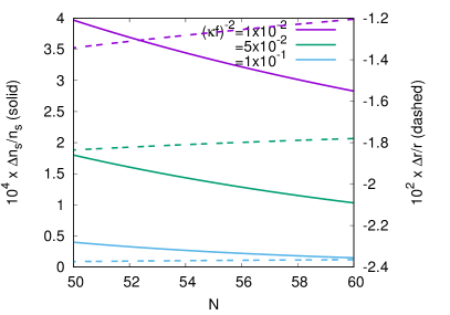
Figure 1: Relative errors in the values of inflationary quantities in case of NI, see Eqs. (21), as calculated from the analytical solution (20) and the numerical one obtained from Eqs. (4). The curves are labeled in terms of the dimensionless quantity $(\kappa f)^{-2}$, where $f$ is the so-called decay constant. The plotted values correspond to the formula $(g^{pert}-g^{num})/g^{num}$, where $g$ can either be the spectral index $n_{S}$ (left vertical axis, solid curves) or the tensor-to-scalar ratio $r$ (right vertical axis, dashed curves). The relative errors are less than $0.04\%$ ($2.4\%$) in the case of $n_{S}$ ($r$) for the values of interest at $N=50-60$ $e$-folds before the end of inflation.

To finish this section, we now show that the simplest inflationary case allowed by our perturbative approach belongs to Class I, and can be obtained from Eq. (20) in the limit $k_{11}\to 3^{+}$:

$$\theta_{N}=\theta_{end}\left[(2k_{13}+1)\theta^{2}_{end}N+1\right]^{-1/2}\,.$$ (23)

One typical example in this case is large field inflation (LFI). The scalar field potential is $V(\phi)=M^{4}(\phi/\phi_{0})^{2n}$Linde (1983), for which we find the following field derivatives:

$$V^{1/2} = M^{2}(\phi/\phi_{0})^{n}\,,$$ (24a)

$$\partial_{\phi}V^{1/2} = nM^{2}\phi^{n-1}/\phi^{n}_{0}\,,$$ (24b)

$$\partial^{2}_{\phi}V^{1/2} = n(n-1)M^{2}\phi^{n-2}/\phi^{n}_{0}\,.$$ (24c)

In terms of the definitions (2b), Eqs. (24) can be combined as $y_{2}=[(1-n)/2n]y^{2}_{1}/y$. Writing the latter expression in terms of the expansion coefficients (5), we find that $k_{20}=0=k_{21}$ and $k_{22}=[(1-n)/2n]k^{2}_{11}$. As before, the same results can be obtained from Eqs. (19) with $\phi_{\rm dS}=-\infty$, which is the critical value of the scalar field indicated by the condition (19a).

If we now use Eqs. (18), we obtain that $k_{11}=3$, $k_{12}=0$, and $k_{13}=3/4n-1/2$. Notice that $k_{13}$ is negative for $n>1$, but the important combination in Eq. (6) is $(k_{13}+1/2)$, which is always positive. If we substitute these values in Eqs. (9) and (23), we find the exact resultsLiddle and Lyth (2000); Martin et al. (2014):

$$1-n_{S}=\frac{3(n+1)}{3N+2n\theta^{-2}_{end}}\,,\quad r=\frac{24n}{3N+2n\theta^{-2}_{end}}\,.$$ (25)

In the limit $n\ll 1$ we find that the predictions are $1-n_{S}=1/N$ and $r=0$; see also Eq. (28) in Sec. V.1 below.

The comparison between the exact numerical solution and the perturbative inflationary one in Eq. (25), in the case of LFI, is shown in Fig. 2. The relative errors of the inflationary quantities are below $0.06\%$ ($1.3\%$) for the spectral index $n_{S}$ (the tensor-to-scalar ratio $r$).

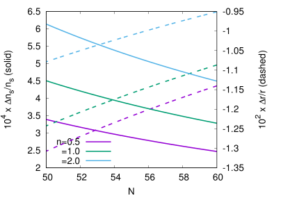
Figure 2: The same as in Fig. 1, but now for the case of LFI, see Eqs. (25). The relative errors between the approximate solution (23) and the exact numerical one is less than $0.06\%$ ($1.3\%$) for $n_{S}$ ($r$) for the values of interest at $N=50-60$ $e$-folds before the end of inflation.

IV.2 Class II: $k_{12}\neq 0$

In principle, this class is defined simply as all inflationary cases of which the solution is given by Eqs. (16) but that do not belong to Class I, which means that $k_{11}\geq 3$, both $k_{12}$ and $k_{13}$ are non-zero, and all three coefficients contribute to the inflationary solution. Unfortunately, there does not seem to be a clear representative example of this general case.

But there is indeed, as in Class I, a particular subclass of solutions within Class II that deserves a separate study. The second- and third-order solutions are

$$\theta^{(2nd)}_{N} = \theta_{end}\left(\theta_{end}k_{12}N+1\right)^{-1}\,,$$ (26a)

$$k_{12}N^{(3rd)} = \frac{1}{\theta_{N}}-\frac{1}{\theta_{end}}-\frac{1}{\theta_{-}}\ln\left(\frac{1-\theta_{-}/\theta_{end}}{1-\theta_{-}/\theta_{N}}\right)\,,$$ (26b)

where $\theta_{-}=-2k_{12}/(2k_{13}+1)$ (and also $\theta_{+}=0$). It can be easily shown that Eqs. (26) can be obtained from the general solution (16) in the limit $k_{11}\to 3^{+}$.

Examples of this subclass are the Starobinsky’s modelStarobinsky (1980) and, more generally, the so-called $\alpha$ attractorsCarrasco et al. (2015); *Kallosh:2013yoa; *Galante:2014ifa (see also the Higgs Inflation model inMartin et al. (2014)). For general purposes of illustration, we write the scalar field potential as $V(\phi)=M^{4}(1-e^{-\lambda\kappa\phi})^{2}$, for which we find

$$V^{1/2} = M^{2}\left(1-e^{\lambda\kappa\phi}\right)\,,$$ (27a)

$$\partial_{\phi}V^{1/2} = -\lambda\kappa M^{2}e^{\lambda\kappa\phi}\,,$$ (27b)

$$\partial^{2}_{\phi}V^{1/2} = -\lambda^{2}\kappa^{2}M^{2}e^{\lambda\kappa\phi}\,,$$ (27c)

where we have changed the conventional signs so that the perturbative solution (6) picks up the correct branch in the potential that corresponds to the de Sitter solution. Otherwise, we would have encountered the power-law solution related to the second critical point in the dynamical system, see Sec. II.2.

Equations (27) suggest that $y_{2}=\sqrt{6}\lambda y_{1}$, which in turn means that $k_{20}=0$, $k_{21}=\sqrt{6}\lambda k_{11}$, and $k_{22}=\sqrt{6}\lambda k_{12}$. From Eqs. (18) we find that $k_{11}=3$, $k_{12}=(\sqrt{6}/2)\lambda$, and $k_{13}=1/4-\lambda^{2}/2$. Needless to say, the same values are also obtained from Eqs. (19) for the de Sitter critical point $\phi_{\rm dS}=-\infty$.

Even though Eq. (26b) is an analytical third-order solution, the one considered in most papers is the second-order one in Eq. (26a)Martin et al. (2014). For the latter, in the large $N$ limit, we find that $\theta_{N}\simeq(1/k_{12})N^{-1}=(2/\sqrt{6}\lambda)N^{-1}$. It is also true that in the limit $\lambda\to 0$ the expansion coefficients are $k_{11}=3$, $k_{12}=0$, and $k_{13}=1/4$, which corresponds to the quadratic potential (see Sec. IV.1 above). These two limiting behaviors of this type of model have been widely studied in the literatureGalante et al. (2014).

The parameter $\theta_{-}$ diverges for $\lambda^{2}=3/2$, and then we find that, in the limit $\lambda\to\sqrt{3/2}$, Eq. (26b) transforms into Eq. (26a). We recall here that the original Starobinsky model corresponds to $\lambda=\sqrt{2/3}$Starobinsky (1980); Ade et al. (2015), and then its solution is well represented by Eq. (26a) with $k_{12}=1$. For values $\lambda^{2}>3/2$ the parameter $\theta_{-}$ becomes negative, and then Eq. (26b) does not give consistent solutions for all cases, which may indicate the need to consider higher-order corrections in the inflationary solution (6).

As we did before for the case of NI, the comparison between the numerical and the perturbative inflationary solutions in the case of the Starobinsky model is shown in Fig. 3. The relative errors of the inflationary quantities is below $0.14\%$ ($6\%$) for the spectral index $n_{S}$ (the tensor-to-scalar ratio $r$). Notice that for simplicity the comparison was made in terms of the second-order perturbative solution in Eq. (26a), but a better result can be obtained if the third-order one in Eq. (26b) is used instead.

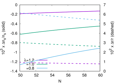
Figure 3: The same as in Figs. 1 and 2, but now for the case of the Starobinsky’s model, see Eqs. (27). The perturbative solutions were calculated from the second-order equation (26a). The curves are labeled in terms of the parameter $\lambda$ that appears in the potential. The relative errors are less than $0.14\%$ ($6\%$) in the case of $n_{S}$ ($r$) for the values of interest at $N=50-60$ $e$-folds before the end of inflation.

V General results on the $n_{S}-r$ plane

In the above sections we discussed the mathematical properties of the general solutions arising from single models of inflation. Those solutions are characterized by three numbers: $k_{11}$, $k_{12}$ and $k_{13}$, and these same numbers are the ones that determine the values of the observables, so that $n_{S}=n_{S}(k_{11},k_{12},k_{13})$, and $r=r(k_{11},k_{12},k_{13})$.

The two classes presented in Sec. IV were each exemplified each one by typical cases that are well known in the literature, but as we shall see now, the capabilities of the inflationary models are more extended than those suggested by the given instances of particular potentials.

The calculations below were made under the assumption that the numbers $k_{11}$, $k_{12}$ and $k_{13}$ are all independent. As we saw before, Eqs. (18) and (19) indicate that they are not completely independent once we choose a particular potential $V(\phi)$, but here we will take a less restrictive point of view, because we only want to make a estimation of the values of $k_{11}$, $k_{12}$ and $k_{13}$ that are in principle compatible with observations.

V.1 Class I

The predictions for the plane $n_{S}-r$ are shown in Fig. 4 for $N=50,60$ $e$-folds before the end of inflation. We can see that if we keep $k_{11}={\rm const}$, the resultant plots are straight lines which are parallel to the one corresponding to $k_{11}=3$. As expected from Eq. (9), this confirms that $k_{11}$ has a major effect on the value of the spectral index $n_{S}$, and then a good fit to the observational data requires that $3.018>k_{11}>3$. This also shows that the value of $k_{11}$ should be away from the slow-roll value $k_{11}=3$, but not by much. On the other hand, the curves that are obtained from $k_{13}={\rm const.}$ are not straight lines, and they show that $k_{13}$ has a major effect in the value of the tensor-to-scalar ratio $r$, and that in principle $k_{13}>0.5$ is required in order to obtain a low enough value of $r$.

Actually, it can be shown that in the limit $k_{13}\to\infty$ of Eq. (20), which should result in a null value of $r$, the prediction for the spectral index is:

$$1-n_{S}\simeq 2(k_{11}-3)+1/N\,.$$ (28)

In the calculation of Eq. (28) we have also considered that $(k_{11}-3)N\ll 1$, which seems to be approximately correct in the cases of interest; see Fig. 4. Equation (28) also suggests that for models in Class I there is an upper bound in the value of the spectral index given by $n_{S}\leq 1-1/N$; this results in $n_{S}\leq 0.98$ if $N=50$ ($n_{S}\leq 0.983$ if $N=60$).

Just for comparison, we also show in Fig. 4 the inflationary results obtained from the LFI ($\phi^{2}$) and the NI potentials. As it is now widely accepted, those potentials seem to be ruled out by observationsMartin et al. (2014). Notice in particular that the curve from the NI potential almost corresponds to an isoline of $k_{13}={\rm const.}$, but the value of the latter is not large enough to be in agreement with the observational constraints.

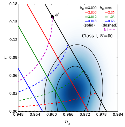
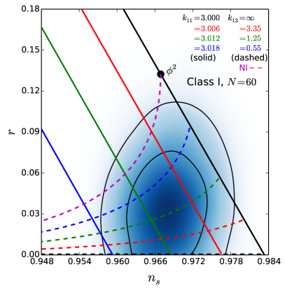
Figure 4: General results on the plane $n_{S}$ vs $r$ for the Class I, from Sec. IV.1, of single-field models of inflation. The plots show the results for $N=50$ (left) and $N=60$ (right). Notice that Class I is not completely ruled out by observations, mostly because it can provide low enough values of the tensor-to-scalar ratio $r$. The predictions from the typical LFI for the potential $\phi^{2}$ [$n=1$ in Eq. (24)], and NI [Eq. (21)], are indicated in the figures for comparison. The contours represent the $65$% and $95$% confidence levels of the Planck TT+lowP+BAO dataAde et al. (2015).

V.2 Class II

For the comparison of this class of inflationary solutions, we will only consider the second-order solutions in Eqs. (16a) and (26a). Although the third-order solutions would be more precise, the second-order ones are accurate enough for the purposes of this section, and they will allow us to show the main results in a similar way as for Class I above. The general predictions from the models in Class II are presented in Fig. 5.

If we keep $k_{11}={\rm const.}$, the resultant plots are straight lines which are parallel to the one corresponding to $k_{11}=3$. This again shows that $k_{11}$ has a major effect on the value of the spectral index $n_{S}$. However, a major difference with respect to Class I appears here: the region covered by Class II in the parameter space moves away considerably from the constrained region if $k_{11}>3$. Hence, the best option here seems to be the slow-roll value $k_{11}=3$. On the other hand, the curves that are obtained from $k_{12}={\rm const.}$ show that $k_{12}$ has a major effect on the value of the tensor-to-scalar ratio $r$ (similar to the role of $k_{13}$ in Class I) and that in principle $k_{12}>0.2$ is required in order to obtain a low enough value of $r$.

A difference with respect to the role of $k_{13}$ in Class I, is that the value of $r$ vanishes more quickly as $k_{12}$ grows, which is explained from the fact that for models in Class II we have that $\theta_{N}\sim N^{-1}$, whereas for those in Class I the result is just $\theta_{N}\sim N^{-1/2}$. This also has a visible effect on the spectral index. If we take the limit $k_{12}\to\infty$ of Eq. (16a), we find that

$$1-n_{S}\simeq 2(k_{11}-3)+2/N\,.$$ (29)

In the calculation of Eq. (29) we have again considered that $(k_{11}-3)N\ll 1$, which seems to be approximately correct in the cases of interest, see Fig. 5. Equation (29) also suggests that for models in Class II there is an upper bound in the value of the spectral index given by $n_{S}\leq 1-2/N$; this results in $n_{S}\leq 0.96$ if $N=50$ ($n_{S}\leq 0.966$ if $N=60$). This in turn indicates that models in Class II can only explore a smaller range of values of $n_{S}$ than those in Class I, and this limitation may put them in jeopardy when compared with observations.

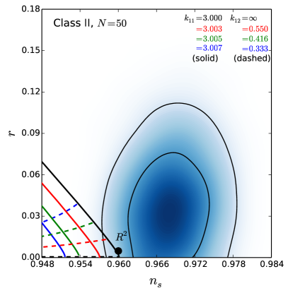
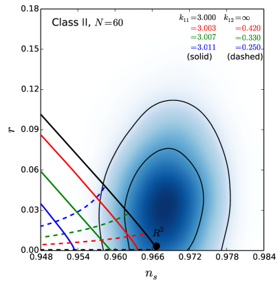
Figure 5: General results on the plane $n_{S}$ vs $r$ for Class II, from Sec. IV.2, of single field models of inflation. The plots show the results for $N=50$ (Left) and $N=60$ (Right). Notice that Class II covers a smaller area than Class I (see Fig. 4), and then it has less freedom to fit the observational data. The predictions from the typical Starobinsky’s model ($R^{2}$) ($\lambda=\sqrt{2/3}$ in Eq. (27)), is indicated in the figures for comparison. The contours represent the $65$% and $95$% confidence levels of the Planck TT+lowP+BAO dataAde et al. (2015).

VI Conclusions

We have presented a new transformation of the equations of motion in single-field inflationary models that render them in a more suitable form for a dynamical system analysis than in other standard approaches. The evolution of the scalar field is given mostly by an internal angle variable $\theta$, which together with other potential variables, allows a perturbative solution around a critical, de Sitter, point at any desirable order.

It must be remarked that the perturbative method does not require the imposition of the slow-roll approximation, and can actually be applied to scalar field models even if the slow-roll conditions are not strictly attained. Also, in contrast to slow roll, the method does not explicitly need to resolve the evolution of the scalar field, and the full solution is just represented by the angular variable $\theta$. Given that $w_{\phi}=-\cos\theta$ (see Sec. II), this illustrates the fact that, for inflationary calculations, the evolution of the equation of state $w_{\phi}$ is all that is required for a full inflationary solution.

In addition, the new equations of motion showed that there are two critical points of physical interest, which in turn suggested that the inflationary solutions appear in two flavors. The first critical point corresponds to power-law inflation, which only appears for a very restricted type of exponential-like potentials. The second critical point corresponds to de Sitter inflation, which is a generic case for a broad range of scalar field potentials, and this is why its solutions were studied more in detail than those of the power-law one.

The main source of error in the inflationary solutions comes precisely from the determination of $\theta_{N}$ itself, the value of the angular variable at a given number of $e$-folds before the end of inflation. The value of $\theta_{N}$ is mainly affected by the truncation in the expansion of $y_{1}$, but we showed that at least in some selected examples the accuracy of the method is good enough. Furthermore, the effect of $\theta_{N}$ is less important in the determination of $n_{S}$, and then the predictions for the spectral index have a much larger accuracy than those for the tensor-to-scalar ratio $r$.

The new method suggests that de Sitter inflation in single-field models can be arranged in two general classes, which we called Class I and Class II, irrespective of the considered scalar field potential. We were able to identify representative examples for each class, although an example that fully shows the features of Class II seems not to have been reported before. Interestingly enough, the key parameter for such a classification is the coefficient $k_{12}$. If we take the large $N$ limit of the two classes, we end up with only two typical behaviors in the solutions, namely, $\theta_{N}\sim N^{-1/2}$ ($k_{12}=0$: Class I) or $\theta_{N}\sim N^{-1}$ ($k_{12}\neq 0$: Class II), which suggests that either $r\sim N^{-1}$ or $r\sim N^{-2}$, respectively, even though $1-n_{S}\sim N^{-1}$ at the leading order in $N$ for the two classes. This is in agreement with recent works that suggest the existence of these universal classes in inflationRoest (2014); *Galante:2014ifa (see also Ref. Mukhanov (2013)). As for the comparison with observations, it seems that models in Classes I are the most suitable to fit the current constraints because of the suppressed value of the tensor-to-scalar ratio $r$, and the more extended freedom to fit the preferred value of the spectral index $n_{S}\simeq 0.965$Ade et al. (2015) [see Eq. (28) above].

The dynamical treatment presented here also showed that the determination of the inflationary quantities $(n_{S},r)$ is insensitive to the energy scale of the scalar field potential, and then the latter may be left out in any fitting analysis. This is not possible, though, in the standard approach to scalar field dynamics, in which none of the potential parameters can be avoided in the calculation of the inflationary trajectories.

A key ingredient in the method was the transformation of the dynamical system into a hierarchy of algebraic relations for the numerical coefficients in a series expansion. We showed that there is a shortcut to solving such an algebraic system for any scalar field potential with a given relation among its first potential variables in the form $f(y,y_{1},y_{2})=0$. This is a relation between the scalar field potential $V(\phi)$ and its first two derivatives through the definitions (2b). The examples we considered above cover some of the most popular instances in recent inflationary studies; see Refs. Ade et al. (2015); Martin et al. (2014); Cook et al. (2015); *Cai:2015soa; *Munoz:2014eqa and references therein. Nonetheless, we showed that there is a general procedure to calculate the expansion coefficients $k_{1j}$ of the potential variable $y_{1}$, as long as one is able to identify the de Sitter critical point in the given scalar field potential. At the end, the method can be applied to a large variety of models, the inflationary solutions of which would belong to those of either Class I or Class II.

The framework presented here can in principle be extended to more general situations, in which the scalar field would be endowed to more complicated potentials. The hierarchy of algebraic equations (18) and (19) will correspondingly become more involved too, but this will not have any effect in our general classification of inflationary cases. The reason is that such classification only depends upon the given value of a single coefficient ($k_{12}$), whatever further complications may arise in the solution of the algebraic hierarchy.

Appendix A Notes on the accuracy of the series expansion in Eq. (5)

A shown in the previous sections, the inflationary solutions of the equations of motion (4), under the ansatz (5) for the potential variabls $y_{I}$, give accurate enough results of the inflationary variables if the series expansion of the first potential variable $y_{1}$ is considered up to the third order. This is also the highest order at which one can find analytical expressions of Eq. (6), namely Eqs. (16).

It is certainly expected that the solutions will improve if more higher-order terms are taken into account, but the question remains of whether there is any a priori assessment of the accuracy of the method, given that at the end of inflation $\theta_{end}=\mathcal{O}(1)$. The following is a brief discussion about this issue.

To begin with, the truncated series expansion $y_{1}\simeq k_{11}\theta+k_{12}\theta^{2}+k_{13}\theta^{3}$ indicates that at the end of inflation $y_{1}(\theta_{end})\sim 3\theta_{end}\simeq 3.69$, with the precise value depending upon the exact form of the potential. The problem is that we do not know beforehand what is the true value of $y_{1}(\theta_{end})$, and then we do not have a value of reference to compare our results with.

The most we can do is to estimate $y_{1}(\theta_{end})$ by other means, like in the case of the slow-roll approximation (SRA). As is known, under the SRA the end of inflation is estimated to happen by the breaking of the slow-roll condition; the latter is given by

$$\epsilon_{V}=\frac{1}{2\kappa^{2}}\left(\frac{\partial_{\phi}V}{V}\right)^{2}=\frac{y^{2}_{1}}{12y^{2}}\simeq 1\,,$$ (30)

where $\epsilon_{V}$ is the so-called first slow-roll parameter. If we assume that Eq. (30) really coincides with the end of inflation at $\theta_{end}$, we find that $y_{1}(\theta_{end})\simeq 2\sqrt{3}\cos(\theta_{end}/2)$. We must notice that the breaking of the slow-roll condition in Eq. (30) is the same for all potentials, which means that under the SRA we must in general expect that $y_{1}(\theta_{end})\simeq 1.15$.

As rough as it is, the slow-roll expression (30) seems to give us a correct order-of-magnitude estimation of the value of $y_{1}$ at the end of inflation. For instance, the end value provided by the aforementioned (truncated) expansion of $y_{1}$ in the case of LFI with $n=1$ is $y_{1}(\theta_{end})=4.16$ (see Sec. IV.1), whereas in the case of Starobinsky’s model we get $y_{1}(\theta_{end})=5.05$ (see Sec. IV.2).

Another hint about the accuracy of the third-order solution comes from the behavior of the series coefficients in Eq. (5). If we rewrite the latter in the case of $y_{1}$ as

$$y_{1}(\theta)=k_{11}\theta\left(1+\frac{k_{12}}{k_{11}}\theta+\frac{k_{13}}{k_{11}}\theta^{2}+\ldots\right)\,,$$ (31)

we can see that the possible convergence of the series (31) depends upon the relative values of the coefficients of higher-order with respect to the first one $k_{11}$. For the same selected examples studied in the main text, we find that

$$\mathrm{NI}: \quad\frac{k_{12}}{k_{11}}=0\,,\;\frac{k_{13}}{k_{11}}=\frac{1}{8}\,,$$ (32a)

$$\mathrm{LFI}(n=1): \quad\frac{k_{12}}{k_{11}}=0\,,\;\frac{k_{13}}{k_{11}}=\frac{1}{12}\,,$$ (32b)

$$\mathrm{Starobinsky}: \quad\frac{k_{12}}{k_{11}}=\frac{1}{3}\,,\;\frac{k_{13}}{k_{11}}=-\frac{1}{36}\,.$$ (32c)

In the case of the value at the end of inflation, $y_{1}(\theta_{end})$, Eqs. (32) seem to indicate that the terms inside the brackets have a decreasing contribution to the total sum. Actually, the third-order term $(k_{13}/k_{11})\theta^{2}_{end}$ in Eq. (31) contributes the most in the case of NI, but only with a correction of about $18$%, and then it is reasonable to think that higher-order terms will have a less important contribution than that.

The same conclusion seems to arise from the general case in Eqs. (18). For the purposes of illustration, we consider that $k_{11}=3$ ($k_{20}=0$), and then

$$\left.\frac{k_{12}}{k_{11}}\right|_{k_{11}=3}=\frac{k_{21}}{18}\,,\quad\left.\frac{k_{13}}{k_{11}}\right|_{k_{11}=3}=\frac{1}{12}-\frac{k^{2}_{21}}{54}+\frac{k_{22}}{6}\,.$$ (33)

Although not a general proof because we lack the information about the coefficients $k_{2j}$ [see Eqs. (19)], Eqs. (33) reinforce the idea that an expansion of $y_{1}$ up to the third order in Eq. (5) may well suffice to obtain accurate enough inflationary solutions.

References

- Ade et al. (2015) P. Ade et al. (Planck Collaboration), (2015), arXiv:1502.02114 [astro-ph.CO] .
- Liddle and Lyth (2000) A. R. Liddle and D. Lyth, Cosmological inflation and large scale structure (2000).
- Mukhanov (2005) V. Mukhanov, Physical foundations of cosmology (2005).
- Malik and Wands (2009) K. A. Malik and D. Wands, Phys.Rept. 475, 1 (2009), arXiv:0809.4944 [astro-ph] .
- Mortonson et al. (2011) M. J. Mortonson, H. V. Peiris, and R. Easther, Phys.Rev. D83, 043505 (2011), arXiv:1007.4205 [astro-ph.CO] .
- Martin et al. (2014) J. Martin, C. Ringeval, and V. Vennin, Phys.Dark Univ. (2014), 10.1016/j.dark.2014.01.003, arXiv:1303.3787 [astro-ph.CO] .
- Martin (2015) J. Martin, (2015), arXiv:1502.05733 [astro-ph.CO] .
- Vennin et al. (2015a) V. Vennin, K. Koyama, and D. Wands, JCAP 1511, 008 (2015a), arXiv:1507.07575 [astro-ph.CO] .
- Vennin et al. (2015b) V. Vennin, K. Koyama, and D. Wands, (2015b), arXiv:1512.03403 [astro-ph.CO] .
- Urena-Lopez (2006) L. A. Urena-Lopez, (2006), arXiv:physics/0609181 [physics] .
- Faraoni and Protheroe (2013) V. Faraoni and C. S. Protheroe, Gen.Rel.Grav. 45, 103 (2013), arXiv:1209.3726 [gr-qc] .
- García-Salcedo et al. (2015) R. García-Salcedo, T. Gonzalez, F. A. Horta-Rangel, I. Quiros, and D. Sanchez-Guzmán, Eur.J.Phys. 36, 025008 (2015), arXiv:1501.04851 [gr-qc] .
- Urena-Lopez and Gonzalez-Morales (2015) L. A. Urena-Lopez and A. X. Gonzalez-Morales, (2015), arXiv:1511.08195 [astro-ph.CO] .
- Copeland et al. (1998) E. J. Copeland, A. R. Liddle, and D. Wands, Phys.Rev. D57, 4686 (1998), arXiv:gr-qc/9711068 [gr-qc] .
- Reyes-Ibarra and Urena-Lopez (2010) M. J. Reyes-Ibarra and L. A. Urena-Lopez, AIP Conf.Proc. 1256, 293 (2010).
- Linder (2010) E. V. Linder, (2010), arXiv:1009.1411 [astro-ph.CO] .
- Rendall (2007) A. D. Rendall, Class.Quant.Grav. 24, 667 (2007), arXiv:gr-qc/0611088 [gr-qc] .
- Alho and Uggla (2014) A. Alho and C. Uggla, (2014), arXiv:1406.0438 [gr-qc] .
- Caldwell and Linder (2005) R. R. Caldwell and E. V. Linder, Phys. Rev. Lett. 95, 141301 (2005), arXiv:astro-ph/0505494 [astro-ph] .
- Liddle et al. (1994) A. R. Liddle, P. Parsons, and J. D. Barrow, Phys.Rev. D50, 7222 (1994), arXiv:astro-ph/9408015 [astro-ph] .
- Lucchin and Matarrese (1985) F. Lucchin and S. Matarrese, Phys. Rev. D32, 1316 (1985).
- Ringstrom (2009) H. Ringstrom, Commun. Math. Phys. 290, 155 (2009).
- Urena-Lopez (2012) L. A. Urena-Lopez, JCAP 1203, 035 (2012), arXiv:1108.4712 [astro-ph.CO] .
- Hoffman and Turner (2001) M. B. Hoffman and M. S. Turner, Phys. Rev. D64, 023506 (2001), arXiv:astro-ph/0006321 [astro-ph] .
- Kinney (2002) W. H. Kinney, Phys. Rev. D66, 083508 (2002), arXiv:astro-ph/0206032 [astro-ph] .
- Liddle (2003) A. R. Liddle, Phys. Rev. D68, 103504 (2003), arXiv:astro-ph/0307286 [astro-ph] .
- Vennin (2014) V. Vennin, Phys. Rev. D89, 083526 (2014), arXiv:1401.2926 [astro-ph.CO] .
- Coone et al. (2015) D. Coone, D. Roest, and V. Vennin, JCAP 1511, 010 (2015), arXiv:1507.00096 [astro-ph.CO] .
- Easther and Peiris (2012) R. Easther and H. V. Peiris, Phys. Rev. D85, 103533 (2012), arXiv:1112.0326 [astro-ph.CO] .
- Freese and Kinney (2014) K. Freese and W. H. Kinney, (2014), arXiv:1403.5277 [astro-ph.CO] .
- Freese et al. (1990) K. Freese, J. A. Frieman, and A. V. Olinto, Phys.Rev.Lett. 65, 3233 (1990).
- Adams et al. (1993) F. C. Adams, J. R. Bond, K. Freese, J. A. Frieman, and A. V. Olinto, Phys.Rev. D47, 426 (1993), arXiv:hep-ph/9207245 [hep-ph] .
- Ross et al. (2016) G. G. Ross, G. German, and J. A. Vazquez, JHEP 05, 010 (2016), arXiv:1601.03221 [astro-ph.CO] .
- Vázquez et al. (2015) J. A. Vázquez, M. Carrillo-González, G. Germán, A. Herrera-Aguilar, and J. C. Hidalgo, JCAP 1502, 039 (2015), [Addendum: JCAP1510,no.10,A01(2015)], arXiv:1411.6616 [astro-ph.CO] .
- Linde (1983) A. D. Linde, Phys.Lett. B129, 177 (1983).
- Starobinsky (1980) A. A. Starobinsky, Phys.Lett. B91, 99 (1980).
- Carrasco et al. (2015) J. J. M. Carrasco, R. Kallosh, and A. Linde, (2015), arXiv:1506.01708 [hep-th] .
- Kallosh et al. (2013) R. Kallosh, A. Linde, and D. Roest, JHEP 1311, 198 (2013), arXiv:1311.0472 [hep-th] .
- Galante et al. (2014) M. Galante, R. Kallosh, A. Linde, and D. Roest, (2014), arXiv:1412.3797 [hep-th] .
- Roest (2014) D. Roest, JCAP 1401, 007 (2014), arXiv:1309.1285 [hep-th] .
- Mukhanov (2013) V. Mukhanov, Eur.Phys.J. C73, 2486 (2013), arXiv:1303.3925 [astro-ph.CO] .
- Cook et al. (2015) J. L. Cook, E. Dimastrogiovanni, D. A. Easson, and L. M. Krauss, (2015), arXiv:1502.04673 [astro-ph.CO] .
- Cai et al. (2015) R.-G. Cai, Z.-K. Guo, and S.-J. Wang, (2015), arXiv:1501.07743 [gr-qc] .
- Munoz and Kamionkowski (2015) J. B. Munoz and M. Kamionkowski, Phys.Rev. D91, 043521 (2015), arXiv:1412.0656 [astro-ph.CO] .