Il n’y a pas de formule analytique pour résoudre les problèmes de débruitage avec pénalité en variation totale, tout comme pour beaucoup d’autres problèmes de parcimonie en analyse. En conséquence, son utilisation pour régulariser un problème inverse conduit à de difficiles problèmes d’optimisation, qui sont souvent résolus par des méthodes de premier ordre. Cependant, lorsque le terme d’attache aux données est très mal conditionné et sans structure simple, comme en imagerie cérébrale, son optimisation est coûteuse. Il convient alors de minimiser le nombre d’itérations globales. Nous présentons pour cela fAASTA, une variante de FISTA qui utilise une optimisation interne pour l’opérateur proximal avec une tolérance adaptative. Nous illustrons son intérêt sur une étude empirique d’un problème de “décodage cérébral”. The total variation (TV) penalty, as many other analysis-sparsity problems, does not lead to separable factors or a proximal operator with a closed-form expression, such as soft thresholding for the $\ell_{1}$ penalty. As a result, in a variational formulation of an inverse problem or statistical learning estimation, it leads to challenging non-smooth optimization problems that are often solved with elaborate single-step first-order methods. When the data-fit term arises from empirical measurements, as in brain imaging, it is often very ill-conditioned and without simple structure. In this situation, in proximal splitting methods, the computation cost of the gradient step can easily dominate each iteration. Thus it is beneficial to minimize the number of gradient steps. We present fAASTA, a variant of FISTA, that relies on an internal solver for the TV proximal operator, and refines its tolerance to balance computational cost of the gradient and the proximal steps. We give benchmarks and illustrations on “brain decoding”: recovering brain maps from noisy measurements to predict observed behavior. The algorithm as well as the empirical study of convergence speed are valuable for any non-exact proximal operator, in particular analysis-sparsity problems.

FAASTA: A fast solver for total-variation regularization of ill-conditioned problems with application to brain imaging

1 Introduction: problem setting

Minimizing a functional using the Total Variation (TV) of an image was originally introduced for denoising purposes [16], but it is useful in more general problems, as a regularization for ill-posed inverse problems. For instance for image reconstruction in computed tomography [18], or in regression or classification settings for brain imaging [13]. In image-recovery applications, unlike with pure prediction problems as in machine learning, optimizing the corresponding cost function to a high tolerance is important (see eg in brain imaging [8]). Indeed, the penalty is most relevant in the ill-conditioned region of the data-fit term. However, this optimization is particularly challenging, as the TV penalty introduces a long-distance coupling across the image in the final solution. This paper studies optimization algorithms for TV-penalized inverse problems with an ill-conditioned and computationally costly data-fit term, as in brain imaging. In particular, we introduce a new variant of FISTA that is well suited to inexact proximal operators.

The TV penalty can be seen as an instance of a wider set of regularizations, analysis sparsity problems [19], that impose sparsity on a linear transformation of the image, as eg in TV-$\ell_{1}$ used in brain imaging [10]. In general, an analysis-sparsity risk-minimization problem is written as

$$\hat{\mathbf{w}}=\underset{\mathbf{w}}{\text{argmin}}\biggl{(}\sum_{i=1}^{n}\mathcal{L}(\mathbf{X}_{i},\mathbf{y}_{\!i},\mathbf{w})+\lambda\|\mathbf{K}\,\mathbf{w}\|_{\bullet}\biggr{)}$$ (1)

where $\mathcal{L}$ is the data-fit term, $\mathbf{K}$ is the “analysis operator”, and $\|{\cdot}\|_{\bullet}$ is a simple sparsity-inducing norm, such as the $\ell_{1}$ or $\ell_{21}$ norm. Often, $\mathbf{K}$ is rank-deficient, as in over-complete dictionaries, and $\mathcal{L}$ is ill-conditioned. Problem (1) is thus a challenging ill-conditioned non-smooth optimization.

With linear models, $\mathbf{X}$ is the design matrix. It is ill-conditioned when different features are heavily correlated. These unfortunate settings often happen when the design matrix results from experimental data, as in brain imaging or genotyping, or for many measurement operators that are nearly blind to some aspects of the weights $\mathbf{w}$, eg the high frequencies in tomography or image deblurring applications. Analysis sparsity is then particularly interesting because it can impose sparsity with $\mathbf{K}$ specifically along those aspects of the weights. For instance TV is edge-preserving: it sharpens some high-frequency features.

2 State of the art optimizers

As the norm $\|.\|_{\bullet}$ is not smooth, standard gradient-based optimization methods cannot be readily used to solve (1). Proximal-gradient methods [15] generalize the gradient step with an implicit subgradient step using the proximal operator, defined by $\operatorname{prox}_{g}(\mathbf{y})=\text{argmin}_{\mathbf{x}}\frac{1}{2}\|\mathbf{y}-\mathbf{x}\|_{2}^{2}+g(\mathbf{x})$.

Proximal iterations

If $f$ is the data-fit term, which we assume smooth, while $g$ is the non-smooth penalty, the simplest method is the Iterative Shrinkage-Thresholding Algorithm (ISTA) [7, 6]: alternating gradient descent on the smooth part and application of the proximal map on the non-smooth part with iterations of

$$\mathbf{w}_{k+1}=\operatorname{prox}_{\frac{1}{L}g}\smash{\left(\mathbf{w}_{k}-\frac{1}{L}\nabla_{\!\mathbf{w}}g(\mathbf{w}_{k})\right)},$$ (2)

where $L$ is the Lipschitz constant of $\nabla_{\!\mathbf{w}}f$. An accelerated gradient method, that is multi-step, can speed up convergence for ill-conditioned problems by adding a momentum term: in the fast iterative shrinkage-thresholding algorithm (FISTA) [3] the gradient steps are applied to a combination of $\mathbf{w}_{k}$ and $\mathbf{w}_{k-1}$. The drawback is that there is no guarantee that each step of FISTA decreases the energy and large rebounds are common. This non-monotone behavior can be remedied by switching to ISTA iterations whenever an increase in cost is detected, as in monotone FISTA (mFISTA) [2].

Proximal algorithms for analysis sparsity

The success of ISTA-type algorithms hinges upon the computation of the proximal operator, that is very efficient for synthesis sparsity as in lasso and elastic-net like problems ($\ell_{1}$ and $\ell_{1}+\ell_{2}$ penalties). However, for many analysis-sparsity proximal operators there is no analytical formula. If the norm used in the analysis sparsity is $\ell_{1}$ or an $\ell_{21}$, writing the dual problem leads to a constraint formulation amenable to an accelerated projected gradient [2], as the dual norms are respectively an $\ell_{\infty}$ and $\ell_{2\infty}$ with easy projections to the unit ball. Importantly, a monotone scheme can also be used, and the tolerance of the optimization can be controlled via the dual gap [13].

While the computation of the proximal operator is no longer exact, proximal gradient algorithms can be shown to converge as long as error on the proximal operation decreases sufficiently with the iteration number $k$ of the outer loop [17]. To achieve the best convergence rates in $k$, the error may be required to decrease as fast as $\varepsilon_{k}\sim k^{-4}$. Using an accelerated algorithm to compute the proximal, achieving a tolerance of $\varepsilon$ is in $\mathcal{O}(\sqrt{\varepsilon})$. Thus, in such a scheme the cost of each iteration increases as $k^{2}$, which renders optimization to a tight tolerance prohibitive.

Operator splitting algorithms

The costly inner loop is required in ISTA-type algorithms because the proximal operator cannot be easily computed on the primal variables of the optimization. Another family of proximal algorithms rely on “splitting”: introducing auxiliary variables in the analysis space: $\mathbf{z}=\mathbf{K}\,\mathbf{w}$. Optimizing on these is then a simple $\ell_{1}$ or $\ell_{21}$ proximal problem. The alternating direction method of multipliers (ADMM) is such an approach that is popular for signal processing applications for its versatility [4]. Note that it relies on the choice of a hyper-parameter, $\mathbf{\rho}$ controlling the tightness of the split that can have an impact on the convergence. Similarly, the primal-dual algorithm in [5] relies on two hyperparameters and can be written as a preconditioned version of ADMM.

Optimizing a smooth surrogate

Newton or quasi-newton algorithms are excellent optimizers for smooth problems that achieve quadratic convergence rates under weak conditions and are somewhat unaffected by ill conditioning [14]. In particular, the limited-memory BFGS (LBFGS) [12] quasi-newton scheme is well suited to high-dimensional problems. An approach to minimizing a convex non-smooth function relies on minimizing series of smooth upper bounds, decreasing the approximation as the algorithm progresses [8, 9]. Intuitively, the benefit of such an approach is that it should be well suited to strong ill-conditioning of the smooth part of the energy, to the cost of more difficulty in optimizing the non-smooth part.

Iteration cost

When the design matrix $\mathbf{X}$ is large and dense, as in brain imaging or genomics, the computation cost of multiplying it with a vector or matrix is by far the most expensive elementary operations as does not fit in $\mathbf{X}$ CPU cache. Thus it is important to limit as much as possible these operations, which typically come into play when computing the gradient or energy of the smooth data-fit part of the problem.

3 FAASTA: adapting inner tolerance

ISTA-type schemes are parameter-free algorithms with a good convergence rate. However their optimal use in analysis-sparsity problems require balancing the computational cost of the gradient step with that of the proximal operator. Indeed, while a tight tolerance on the proximal operator may guarantee the optimal convergence speed in terms of number of iterations of the outer loop, it implies increasing computing time for each iteration. Thus, for a low desired tolerance on the global energy function, it may be beneficial to set a lax tolerance on the dual gap of the proximal operator, and thus achieve fast iterates. On the opposite, optimizing the global problem to a stringent tolerance requires very high precision on the proximal operator, which in turn slows down iterations of the outer loop.

Algorithm 1 fAASTA

$\mathbf{w}_{0}$

$\text{ISTA}\leftarrow False,\qquad$ $\mathbf{v}_{1}\leftarrow\mathbf{w}_{0},\qquad$ $k\leftarrow 0,\qquad$

$t_{1}\leftarrow 1,\qquad$ $dgtol\leftarrow 0.1$ 

while not converged do

   $k\leftarrow k+1,\quad$

   $\mathbf{w}_{k}\leftarrow\operatorname{prox}_{\frac{g}{L}}(\mathbf{v}_{k}-\frac{1}{L}\nabla f(\mathbf{v}_{k}),dgtol)$ 

   if $\mathcal{E}(\mathbf{w}_{k})>\mathcal{E}(\mathbf{w}_{k-1})$ then

     $\mathbf{w}_{k}\leftarrow\mathbf{w}_{k-1},\qquad$ $\mathbf{v}_{k}\leftarrow\mathbf{w}_{k-1}$ 

     if ISTA then

        $dgtol\leftarrow dgtol/5$ 

        while 

          $\mathcal{E}(\operatorname{prox}_{\frac{g}{L}}(\mathbf{v}_{k}-\frac{1}{L}\nabla_{\!\mathbf{w}}f(\mathbf{v}_{k}),dgtol))>\mathcal{E}(\mathbf{w}_{k-1})$ do

          $dgtol\leftarrow dgtol/5$              $\text{ISTA}\leftarrow True$ 

   else

     if ISTA then

        $\mathbf{v}_{k}\leftarrow\mathbf{w}_{k},\qquad$ $\text{ISTA}\leftarrow False$

     else

        $t_{k}\leftarrow\frac{1+\sqrt{1+4t_{k-1}^{2}}}{2},\qquad$

        $\mathbf{v}_{k}\leftarrow\mathbf{w}_{k}+\frac{t_{k-1}-1}{t_{k}}(\mathbf{w}_{k}-\mathbf{w}_{k-1})$          

We introduce a new variant of ISTA, fast Adaptively Accurate Shrinkage Thresholding Algorithm (fAASTA). The core idea is to adapt the tolerance of the proximal operator as needed for convergence. For this, we rely on the fact that in an ISTA iteration –eq. (2)– the global energy must decrease [7]. Thus we adapt the tolerance of the proximal-operator solver to ensure this decrease. In practice, in the inner loop, we control that tolerance by checking the dual gap of the proximal optimization problem, which is much cheaper to compute than the global energy, as it does not involve the accessing the large, dense design matrix $\mathbf{X}$. We decrease this dual gap setting by a factor of 5 when we observe that an ISTA iteration did not result in an energy decrease. In addition, to benefit from accelerated schemes as in FISTA, we rely on an mFISTA strategy: we apply FISTA iterations but when the energy increases, switch to an ISTA step, in which we can then, if needed, decrease the tolerance on the inner dual gap.

The actual procedure is described in alg. 1. One difficulty is implementing the back and forth between ISTA and FISTA without recomputing intermediate variables. With speed in mind, another important implementation aspect is to factor out expressions common to the gradient and energy computations in order to access the large $\mathbf{X}$ matrix as little as possible. These breakdowns are not detailed here.

4 Empirical study: TV-$\ell_{1}$ for decoding

Here, we benchmark the various algorithms on a brain-decoding application: the task is to predict subject’s behavior, encoded as a categorical variable in $\mathbf{y}$, from fMRI images that constitute the design matrix $\mathbf{X}$. For this purpose, we use a TV-$\ell_{1}$-penalized logistic regression, which is written as an analysis sparsity problem in notations of eq. (1):

loss $$\mathcal{L}(\mathbf{X}_{i},\mathbf{y}_{\!i},\mathbf{w}) =\log\bigl{(}1+\exp\bigl{(}-\mathbf{y}_{\!i}(\langle\mathbf{X}_{i},\mathbf{w}\rangle+b)\bigr{)}\bigr{)}$$ (3)

penalty $$\|\mathbf{K}\,\mathbf{w}\|_{\bullet} =(1-\alpha)\|\nabla\mathbf{w}\|_{21}+\alpha\|\mathbf{w}\|_{1}$$ (4)

where $\nabla$ is the image-domain finite difference operator and the $\ell_{21}$ norm groups the different image directions for an isotrope TV formulation. We set $\alpha=.25$. We investigate discrimination of whether the subject is presented images of shoes or scrambled pictures in a study of human vision, using the data from [11]. We rely on the nilearn library for data download, loading and cleaning [1].

We study convergence of the following approaches: ISTA and mFISTA schemes with i) a lax dual-gap tolerance ($.1$) on the inner problem, ii) a tight dual-gap tolerance ($10^{-10}$), iii) an adaptive control of the dual-gap tolerance as exposed above, and iv) the decrease motivated theoretically in [17]; an LBFGS optimizer on a series of smooth upper-bounds following the approach of [8]; an ADMM with different values of the $\rho$ control parameter (implemented as in [8]).

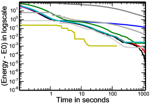
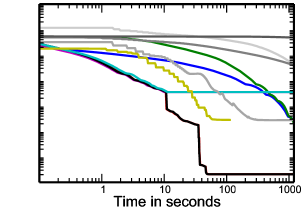
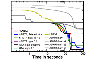
$\lambda=0.0143$                                        $\lambda=1.43$                                        $\lambda=14.3$

Figure 1: Convergence of the different optimization algorithms, for 3 scenarios, with weak, medium and strong regularization, where medium regularization corresponds to the value chosen by cross-validation. These are log-log plots with the 0 defined as the lowest energy value reached across all algorithms.

For all algorithms, we investigate convergence for 3 different values of the regularization parameter, centered around the value minimizing prediction error as measured by cross-validation. On fig. 1, we report energy as a function of time. Importantly, we report time, and not iteration number. Indeed, not only is computing time the most important quantity for the user, but also it is suitable to compare different algorithms.

We find that, as expected, ISTA or FISTA with a lax tolerance on the inner problem reaches an energy plateau before convergence although, for weak to medium regularization, it progresses fast before hitting this limitation. On the opposite, setting a stringent tolerance leads to a slow but steady decrease of the energy (though it eventually also reaches a plateau before complete convergence in the high-regularization case). The theoretical decrease on the tolerance has an intermediate behavior. In particular, it does not stagnate. The convergence of the ADMM approach depends strongly on its control parameter: on the one hand, no control parameter achieves satisfying convergence for all regularization values, on the other hand the ADMM does not converge at all for a bad choice of the parameter. LBFGS reaches a plateau, but gets there fast in the case of weak regularization. Finally, our adaptive approach, whether in its accelerate form, or simply in an ISTA loop, reaches the lowest energy value.

5 Discussion and conclusions

Optimizing an analysis-sparsity functional with a ill-conditioned data-fit term is a very challenging problem as the non-smooth part cannot be readily written as a proximal problem with an analytic solution. Splitting approaches with auxiliary variables in the analysis space are often put forward as a solution for these problems as the non-smooth contribution is easy to solve on these variables. However, when the computation cost of the smooth data-fit part is high, eg when the design matrix is dense and large as in brain imaging, our experience is that these approaches are sub-optimal –see also [8], that explored the preconditioned variant of [5]. We conjecture that in these situations, the choice of the control parameter becomes crucial to accelerate the convergence.

Our preferred solution relies on using an inexact proximal operator and adapting ISTA-type algorithms to set the corresponding tolerance. Experiments show that this approach is robust and always converges to a high tolerance. For very low regularization, the smooth data-fit part of the functional dominates and careful use of smooth optimization methods can achieve a quicker initial rate of convergence but are eventually limited. We currently lack theory on the optimal strategy to set the tolerance of the inner problem. Indeed, on the experiment studied in this contribution, the accelerated gradient variant of the algorithm did not outperform the single-step variant.

Analysis sparsity can be used to capture structure in a much wider set of situations than the simpler, more common synthesis sparsity. However it is seldom used in practice, likely because of the computational cost it entails. Many problems can benefit from faster solvers outside of brain imaging, for instance in tomography image recovery [18].

References

- [1] A. Abraham, F. Pedregosa, M. Eickenberg, et al. Machine learning for neuroimaging with scikit-learn. Frontiers in neuroinformatics, 8, 2014.
- [2] A. Beck and M. Teboulle. Fast gradient-based algorithms for constrained total variation image denoising and deblurring problems. IEEE Trans. Image Proc., 2009.
- [3] A. Beck and M. Teboulle. A fast iterative shrinkage-thresholding algorithm with application to linear inverse problems, 2009.
- [4] S. Boyd, N. Parikh, E. Chu, B. Peleato, and J. Eckstein. Distributed optimization and statistical learning via the alternating direction method of multipliers. Foundations and Trends in Machine Learning, 3:1, 2011.
- [5] A. Chambolle and T. Pock. A first-order primal-dual algorithm for convex problems with applications to imaging. J. Math. Imaging Vis., 40:120, 2011.
- [6] P. L. Combettes and J.-C. Pesquet. Proximal splitting methods in signal processing, 2011.
- [7] I. Daubechies, M. Defrise, and C. De Mol. An iterative thresholding algorithm for linear inverse problems with a sparsity constraint. Communications on pure and applied mathematics, 57:1413, 2004.
- [8] E. Dohmatob, A. Gramfort, B. Thirion, and G. Varoquaux. Benchmarking solvers for TV-l1 least-squares and logistic regression in brain imaging. PRNI, 2014.
- [9] M. Dubois, F. Hadj-Selem, T. Lofstedt, M. Perrot, C. Fischer, V. Frouin, and E. Duchesnay. Predictive support recovery with TV-elastic net penalty and logistic regression: an application to structural MRI. In PRNI, 2014.
- [10] A. Gramfort, B. Thirion, and G. Varoquaux. Identifying predictive regions from fMRI with TV-L1 prior. In PRNI, page 17, 2013.
- [11] J. Haxby, I. Gobbini, M. Furey, et al. Distributed and overlapping representations of faces and objects in ventral temporal cortex. Science, 293:2425, 2001.
- [12] D. C. Liu and J. Nocedal. On the limited memory BFGS method for large scale optimization. Mathematical programming, 45:503, 1989.
- [13] V. Michel, A. Gramfort, G. Varoquaux, et al. Total variation regularization for fMRI-based prediction of behavior. Trans Medical Imaging, 30:1328, 2011.
- [14] J. Nocedal and S. J. Wright. Numerical Optimization. Springer, 2006.
- [15] N. Parikh and S. Boyd. Proximal algorithms. Foundations and Trends in optimization, 1:123, 2013.
- [16] L. I. Rudin, S. Osher, and E. Fatemi. Nonlinear total variation based noise removal algorithms. Physica D, 60:259, 1992.
- [17] M. Schmidt, N. L. Roux, and F. R. Bach. Convergence rates of inexact proximal-gradient methods for convex optimization. In NIPS, page 1458. 2011.
- [18] E. Y. Sidky and X. Pan. Image reconstruction in circular cone-beam computed tomography by constrained, total-variation minimization. Physics in medicine and biology, 53:4777, 2008.
- [19] S. Vaiter, G. Peyré, and J. Fadili. Low complexity regularization of linear inverse problems. arXiv:1407.1598.